Randomized algorithms for low-rank matrix factorizations: sharp performance bounds

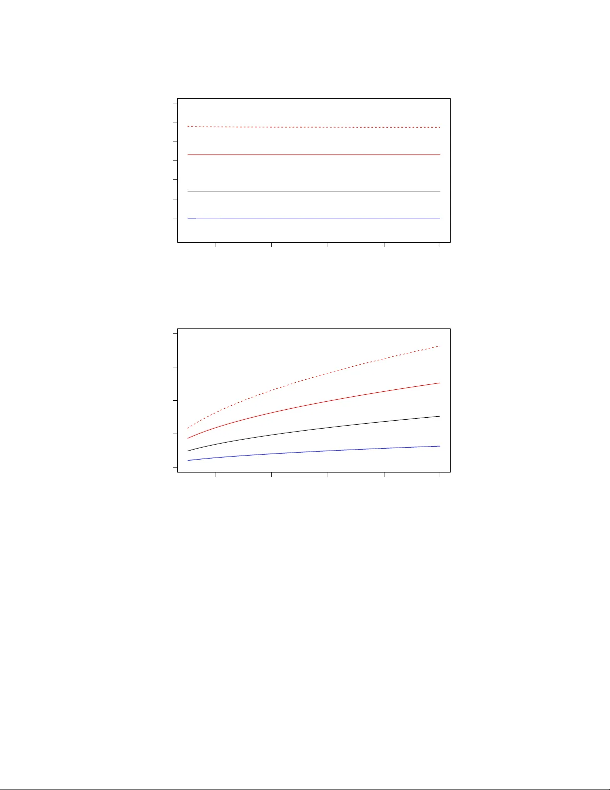
Randomized Algorithms for Lo w-Rank Matrix F actorizations: Sharp P erformance Bounds Rafi Witten ∗ and Emman uel Cand` es † August 2013 Abstract The dev elopment of randomized algorithms for n umerical linear algebra, e.g. for computing appro ximate QR and SVD factorizations, has recen tly become an intense area of research. This pap er studies one of the most frequen tly discussed algorithms in the literature for dimension- alit y reduction—sp ecifically for approximating an input matrix with a lo w-rank element. W e in tro duce a nov el and rather intuitiv e analysis of the algorithm in [6], which allows us to derive sharp estimates and giv e new insights ab out its p erformance. This analysis yields theoretical guaran tees ab out the approximation error and at the same time, ultimate limits of p erformance (lo wer b ounds) showing that our upp er b ounds are tigh t. Numerical exp erimen ts complement our study and sho w the tightness of our predictions compared with empirical observ ations. 1 In tro duction Almost an y metho d one can think of in data analysis and scientific computing relies on matrix algorithms. In the era of ‘big data’, we m ust no w routinely deal with matrices of enormous sizes and reliable algorithmic solutions for computing solutions to least-squares problems, for computing appro ximate QR and SVD factorizations and other such fundamen tal decomp ositions are urgently needed. F ortunately , the dev elopment of randomized algorithms for numerical linear algebra has seen a new surge in recen t years and we b egin to see computational to ols of a probabilistic nature with the p otential to address some of the great challenges p osed by big data. In this pap er, we study one of the most frequen tly discussed algorithms in the literature for dimensionalit y reduction, and pro vide a nov el analysis whic h gives sharp p erformance b ounds. 1.1 Appro ximate lo w-rank matrix factorization W e are concerned with the fundamental problem of approximately factorizing an arbitrary m × n matrix A as A ≈ B C m × n m × ` ` × n (1.1) where ` ≤ min( m, n ) = m ∧ n is the desired rank. The goal is to compute B and C suc h that A − B C is as small as p ossible. Typically , one measures the quality of the appro ximation by taking either ∗ Bit Bo dy , Inc., Cambridge, MA † Departmen ts of Mathematics and of Statistics, Stanford Universit y , Stanford CA 1 the sp ectral norm k · k (the largest singular v alue, also known as the 2 norm) or the F rob enius norm k · k F (the ro ot-sum of squares of the singular v alues) of the residual A − B C . It is well-kno wn that the b est rank- ` approximation, measured either in the sp ectral or F rob enius norm, is obtained by truncating the singular v alue decomp osition (SVD), but this can b e prohibitiv ely exp ensive when dealing with large matrix dimensions. Recen t work [6] in tro duced a randomized algorithm for matrix factorization with low er compu- tational complexit y . Algorithm 1 Randomized algorithm for matrix approximation Require: Input: m × n matrix A and desired rank ` . Sample an n × ` test matrix G with indep endent mean-zero, unit-v ariance Gaussian entries. Compute H = AG . Construct Q ∈ R m × ` with columns forming an orthonormal basis for the range of H . return the appro ximation B = Q , C = Q ∗ A . The algorithm is simple to understand: H = AG is an appro ximation of the range of A ; w e therefore pro ject the columns of A onto this appro ximate range by means of the orthogonal pro jector QQ ∗ and hop e that A ≈ B C = QQ ∗ A . Of natural in terest is the accuracy of this pro cedure: how large is the size of the residual? Sp ecifically , ho w large is k ( I − QQ ∗ ) A k ? The sub ject of the b eautiful surv ey [3] as well as [6] is to study this problem and provide an analysis of p erformance. Before we state the sharp est results known to date, we first recall that if σ 1 ≥ σ 2 ≥ . . . ≥ σ m ∧ n are the ordered singular v alues of A , then the b est rank- ` approximation ob eys min {k A − B k : rank( B ) ≤ ` } = σ ` +1 . It is kno wn that there are choices of A such that E k ( I − QQ ∗ ) A k is greater than σ ` +1 b y an arbitrary m ultiplicative factor, see e.g. [3]. F or example, setting A =  t 0 0 1  and ` = 1, direct c omputation sho ws that lim t →∞ E k ( I − QQ ∗ ) A k = ∞ . Thus, we write ` = k + p (where p > 0) and seek b and b suc h that b ( m, n, k , p ) ≤ sup A ∈ R m × n E k ( I − QQ ∗ ) A k /σ k +1 ≤ b ( m, n, k , p ) . W e are now ready to state the b est results concerning the p erformance of Algorithm 1 we are a ware of. Theorem 1.1 ([3]) . L et A b e an m × n matrix and run A lgorithm 1 with ` = k + p , then E k ( I − QQ ∗ ) A k ≤  1 + 4 √ k + p p − 1 √ m ∧ n  σ k +1 . (1.2) It is a priori unclear whether this upp er b ound correctly predicts the exp ected b ehavior or not. That is to sa y , is the dep endence up on the problem parameters in the righ t-hand side of the righ t order of magnitude? Is the b ound tight or can it b e substan tially impro ved? Are there low er b ounds whic h w ould pro vide ultimate limits of performance? The aim of this pap er is merely to pro vide some definite answers to such questions. 2 1.2 Sharp b ounds It is conv enien t to write the residual in Algorithm 1 as f ( A, G ) := ( I − QQ ∗ ) A as to mak e the dep endence on the random test matrix G explicit. Our main result states that there is an explicit random v ariable whose size completely determines the accuracy of the algorithm. This statement uses a natural notion of sto chastic ordering; b elo w we write X d ≥ Y if and only if the random v ariables X and Y ob ey P ( X ≥ t ) ≥ P ( Y ≥ t ) for all t ∈ R . Theorem 1.2. Supp ose without loss of gener ality that m ≥ n . Then in the setup of The or em 1.1, for e ach matrix A ∈ R m × n , k ( I − QQ ∗ ) A k d ≤ σ k +1 W , wher e W is the r andom variable W = k f ( I n − k , X 2 )  X 1 Σ − 1 I n − k  k ; (1.3) her e, X 1 and X 2 ar e r esp e ctively ( n − k ) × k and ( n − k ) × p matric es with i.i.d. N (0 , 1) entries, Σ is a k × k diagonal matrix with the singular values of a ( k + p ) × k Gaussian matrix with i.i.d. N (0 , 1) entries, and I n − k is the ( n − k ) -dimensional identity matrix. F urthermor e, X 1 , X 2 and Σ ar e al l indep endent (and indep endent fr om G ). In the other dir e ction, for any  > 0 , ther e is a matrix A with the pr op erty k ( I − QQ ∗ ) A k d ≥ (1 −  ) σ k +1 W . In p articular, this gives sup A E k ( I − QQ ∗ ) A k /σ k +1 = E W . The pro of of the theorem is in Section 2.3. T o obtain very concrete b ounds from this theorem, one can imagine using Mon te Carlo simulations by sampling from W to estimate the w orst error the algorithm commits. Alternativ ely , one could derive upp er and low er b ounds ab out W by analytic means. The corollary b elo w is established in Section 2.4. Corollary 1.3 ( Nonasymptotic b ounds). With W as in (1.3) (r e c al l n ≤ m ), p n − ( k + p + 2) E k Σ − 1 k ≤ E W ≤ 1 +  √ n − k + √ k  E k Σ − 1 k . (1.4) In the regime of in terest where n is v ery large and k + p  n , the ratio b etw een the upp er and low er b ound is practically equal to 1 so our analysis is very tight. F urthermore, Corollary 1.3 clearly emphasizes why w e would w ant to take p > 0. Indeed, when p = 0, Σ is square and nearly singular so that b oth E k Σ − 1 k and the lo wer b ound b ecome v ery large. In con trast, increasing p yields a sharp decrease in E k Σ − 1 k and, th us, improv ed p erformance. It is further p ossible to derive explicit b ounds by noting (Lemma A.2) that 1 √ p + 1 ≤ E k Σ − 1 k ≤ e √ k + p p . (1.5) Plugging the righ t inequalit y in to (1.4) impro v es up on (1.2) from [3]. In the regime where k + p  n (w e assume throughout this section that n ≤ m ), taking p = k , for instance, yields an upp er b ound roughly equal to e p 2 n/k ≈ 3 . 84 p n/k and a low er b ound roughly equal to p n/k , see Figure 1. 3 When k and p are reasonably large, it is well-kno wn (see Lemma A.3) that σ min (Σ) ≈ p k + p − √ k so that in the regime of interest where k + p  n , b oth the lo wer and upp er b ounds in (1.4) are ab out equal to √ n √ k + p − √ k . (1.6) W e can formalize this as follows: in the limit of large dimensions where n → ∞ , k , p → ∞ with p/k → ρ > 0 (in suc h a wa y that lim sup ( k + p ) /n < 1), w e hav e almost surely lim sup W b ( n, k , p ) ≤ 1 , b ( n, k , p ) = √ n − k + √ k √ k + p − √ k . (1.7) Con versely , it holds almost surely that lim inf W b ( n, k , p ) ≥ 1 , b ( n, k , p ) = √ n − k − p √ k + p − √ k . (1.8) A short justification of this limit b ehavior may also b e found in Section 2.4. 1.3 Inno v ations Whereas the analysis in [3] uses sophisticated concepts and to ols from matrix analysis and from p erturbation analysis, our metho d is differen t and only uses elementary ideas (for instance, it should b e understandable b y an undergraduate studen t with no sp ecial training). In a n utshell, the authors in [3] control the error of Algorithm 1 b y establishing an upp er b ound ab out k f ( A, X ) k holding for all matrices X (the b ound dep ends on X ). F rom this, they deduce b ounds ab out k f ( A, G ) k in exp ectation and in probabilit y b y integrating with resp ect to G . A limitation of this approac h is that it do es not provide any estimate of how close the upp er b ound is to b eing tigh t. In contrast, we p erform a sequence of reductions, whic h ultimately iden tifies the w orst-case input matrix. The crux of this reduction is a monotonicity prop ert y , whic h roughly sa ys that if the sp ectrum of a matrix A is larger than that of another matrix B , then the singular v alues of the residual f ( A, G ) are sto c hastically greater than those of f ( B , G ), see Lemma 2.1 in Section 2.1 for details. Hence, applying the algorithm to A results in a larger error than when the algorithm is applied to B . In turn, this monotonicit y property allo ws us to write the w orst-case residual in a v ery concrete form. With this represen tation, we can recov er the deterministic b ound from [3] and immediately see the extent to which it is sub-optimal. Most imp ortantly , our analysis admits matc hing low er and upp er b ounds as discussed earlier. Our analysis of Algorithm 1, presented in Section 2.3, sho ws that the approximation error is hea vily affected by the spectrum of the matrix A past its first k + 1 singular v alues. 1 In fact, suppose m ≥ n and let D n − k b e the diagonal matrix of dimension n − k equal to diag( σ k +1 , σ k +2 , . . . , σ n ). Then our metho d sho w that the w orst case error for matrices with this tail sp ectrum is equal to the random v ariable W ( D n − k ) = k f ( D n − k , X 2 )  X 1 Σ − 1 I n − k  k . In turn, a v ery short argument gives the exp ected upp er b ound b elow: 1 T o accommo date this, previous works also provide b ounds in terms of the singular v alues of A past σ k +1 . 4 Theorem 1.4. T ake the setup of The or em 1.1 and let σ i b e the i th singular value of A . Then E k ( I − QQ ∗ ) A k ≤  1 + s k p − 1  σ k +1 + E k Σ − 1 k s X i>k σ 2 i . (1.9) Substituting E k Σ − 1 k with the upp er b ound in (1.5) r e c overs The or em 10.6 fr om [3]. This b ound is tigh t in the sense that setting σ k +1 = σ k +2 = . . . = σ n = 1 essentially yields the upp er b ound from Corollary 1.3, which as we hav e seen, cannot b e improv ed. 1.4 Exp erimen tal results T o examine the tigh tness of our analysis of p erformance, we apply Algorithm 1 to the ‘worst-case’ input matrix and compute the sp ectral norm of the residual, p erforming such computations for fixed v alues of m , n , k and p . W e wish to compare the sampled errors with our deterministic upp er and low er b ounds, as w ell as with the previous upp er b ound from Theorem 1.1 and our error pro xy (1.6). Because of Lemma 2.2, the w orst-case b ehavior of the algorithm do es not dep end on m and n separately but only on min( m, n ). Hence, w e set m = n in this section. Figure 1 reveals that the new upp er and low er b ounds are tight up to a small multiplicativ e factor, and that the previous upp er b ound is also fairly tight. F urther, the plots also demonstrate the effect of concentration in measure—the outcomes of different samples each lie remark ably close to the yello w rule of thum b, esp ecially for larger n , suggesting that for practical purp oses the algorithm is deterministic. Hence, these experimental results reinforce the practical accuracy of the error proxy (1.6) in the regime k + p  n since we can see that the worst-case error is just ab out (1.6). Figure 2 gives us a sense of the v ariabilit y of the algorithm for tw o fixed v alues of the triple ( n, k , p ). As exp ected, as k and p gro w the v ariability of the algorithm decreases, demonstrating the effect of concen tration of measure. 1.5 Complemen ts In order to make the paper a little more self-contained, w e briefly review some of the literature as to explain the cen trality of the range finding problem (Algorithm 1). F or instance, supp ose w e wish to construct an appro ximate SVD of a very large matrix m × n matrix A . Then this can b e ac hieved b y running Algorithm 1 and then computing the SVD of the ‘small’ matrix C = Q ∗ A , c heck Algorithm 2 b elow, whic h returns an approximate SVD A ≈ U Σ V ∗ . Assuming the extra steps in Algorithm 2 are exact, we hav e k A − U Σ V ∗ k = k A − Q ˆ U Σ V ∗ k = k A − QC k = k A − QQ ∗ A k (1.10) so that the appro ximation error is that of Algorithm 1 whose study is the sub ject of this pap er. The p oint here of course is that since the matrix C = Q ∗ A is ` × n —we typically ha ve `  n — the computational cost of forming its SVD is on the order of O ( ` 2 n ) flops and fairly minimal. (F or reference, we note that there is an even more effective single-pass v arian t of Algorithm 2 in whic h w e do not need to re-access the input matrix A once Q is av ailable, please see [3] and references therein for details.) 5 (a) k = p = 0 . 01 n 2e+04 4e+04 6e+04 8e+04 1e+05 0 10 20 30 40 50 60 70 n Approximation error ● ● ● ● ● ● ● ● ● ● ● ● ● ● ● ● ● ● ● ● ● ● ● ● ● ● ● ● ● ● ● ● ● ● ● ● ● ● ● ● ● ● ● ● ● ● ● ● ● ● ● ● ● ● ● ● ● ● ● ● ● ● ● ● ● ● ● ● ● ● ● ● ● ● ● ● ● ● ● ● ● ● ● ● ● ● ● ● ● ● (b) k = p = 100 2e+04 4e+04 6e+04 8e+04 1e+05 0 50 100 150 200 n Approximation error ● ● ● ● ● ● ● ● ● ● ● ● ● ● ● ● ● ● ● ● ● ● ● ● ● ● ● ● ● ● ● ● ● ● ● ● ● ● ● ● ● ● ● ● ● ● ● ● ● ● ● ● ● ● ● ● ● ● ● ● ● ● ● ● ● ● ● ● ● ● ● ● ● ● ● ● ● ● ● ● ● ● ● ● ● ● ● ● ● ● Figure 1: Sp e ctr al norm k ( I − QQ ∗ ) A k of the r esidual with worst-c ase matrix of dimension n × n as input with n varying b etwe en 10 4 and 10 5 . Each gr ey dot r epr esents the err or of one run of A lgorithm 1. The lines ar e b ounds on the sp e ctr al norm: the r e d dashe d line plots the pr evious upp er b ound (1.2) . The r e d (r esp. blue) solid line is the upp er (r esp. lower) b ound c ombining Cor ol lary 1.3 and (1.5) . The black line is the err or pr oxy (1.6) . In the top plot, k = p = 0 . 01 n . Ke eping fixe d r atios r esults in c onstant err or. Holding k and p fixe d in the b ottom plot while incr e asing n r esults in appr oximations of incr e asing err or. Naturally , w e may wish to compute other types of approximate matrix factorizations of A such as eigenv alue decomp ositions, QR factorizations, interpolative decomp ositions (where one searc hes 6 (a) m = n = 10 5 , k = p = 10 2 Approximation error W Frequency 60 65 70 75 80 85 0 20 40 60 80 100 (b) m = n = 10 5 , k = p = 10 3 Approximation error W Frequency 22.5 23.0 23.5 24.0 24.5 0 20 40 60 80 100 Figure 2: We fix n (r e c al l that m = n ), k and p and plot the appr oximation err or W acr oss 1000 indep endent runs of the algorithm. F or the lar ger value of k and p , we se e r e duc e d variability—the appr oximation err ors r ange fr om ab out 61 to 85 for k = p = 10 2 and 22 . 5 to 24 . 5 for k = p = 10 3 , much less variability in b oth absolute and p er c entage terms. Similarly, the empiric al standar d deviation with k = p = 10 2 is appr oximately 3 . 6 while with k = p = 10 3 it fal ls to . 32 . Algorithm 2 Randomized algorithm for approximate SVD computation Require: Input: m × n matrix A and desired rank ` . Run Algorithm 1. Compute C = Q ∗ A . Compute the SVD of C = ˆ U Σ V ∗ . return the appro ximation U = Q ˆ U , Σ, V . for an appro ximation A ≈ B C in whic h B is a subset of the columns of A ), and so on. All suc h computations w ould follow the same pattern: (1) apply Algorithm 1 to find an appro ximate range, and (2) p erform classical matrix factorizations on a matrix of reduced size. This general strategy , namely , appro ximation follow ed b y standard matrix computations, is of course hardly anything new. T o b e sure, the classical Businger-Golub algorithms for computing partial QR decompositions follo ws this pattern. Again, we refer the interested reader to the survey [3]. W e hav e seen that when the input matrix A do es not hav e a rapidly decaying sp ectrum, as this ma y b e the case in a n umber of data analysis applications, the error of approximation Algorithm 1 commits—the random v ariable W in Theorem 1.2—may b e quite large. In fact, when the singular v alues hardly decay at all, it typically is on the order of the error proxy (1.6). This results in p o or p erformance. On the other hand, when the singular v alues decay rapidly , we ha ve seen that the algorithm is prov ably accurate, compare Theorem 1.4. This suggests using a p o wer iteration, similar to the blo ck pow er method, or the subspace iteration in numerical linear algebra: Algorithm 3 w as prop osed in [7]. The idea in Algorithm 3 is of course to turn a slowly decaying sp ectrum into a rapidly decaying 7 Algorithm 3 Randomized algorithm with p ow er trick for matrix approximation Require: Input: m × n matrix A and desired rank ` . Sample an n × ` test matrix G with indep endent mean-zero, unit-v ariance Gaussian entries. Compute H = ( AA ∗ ) q AG . Construct Q ∈ R m × ` with columns forming an orthonormal basis for the range of H . return the appro ximation B = Q , C = Q ∗ A . one at the cost of more computations: we need 2 q + 1 matrix-matrix multiplies instead of just one. The b enefit is improv ed accuracy . Letting P b e any orthogonal pro jector, then a sort of Jensen inequalit y states that for any matrix A , k P A k ≤ k P ( AA ∗ ) q A k 1 / (2 q +1) , see [3] for a pro of. Therefore, if Q is computed via the p ow er tric k (Algorithm 3), then k ( I − QQ ∗ ) A k ≤ k ( I − QQ ∗ )( AA ∗ ) q A k 1 / (2 q +1) . This immediately giv es a corollary to Theorem 1.2. Corollary 1.5. L et A and W b e as in The or em 1.2. Applying Algorithm 3 yields k ( I − QQ ∗ ) A k d ≤ σ k +1 W 1 / (2 q +1) . (1.11) It is amusing to note that with, say , n = 10 9 , k = p = 200, and the error pro xy (1.6) for W , the size of the error factor W 1 / (2 q +1) in (1.11) is ab out 3.41 when q = 3. F urther, w e would lik e to note that our analysis exhibits a sequence of matrices (2.1) that hav e appro ximation errors that limit to the worst case approximation error when q = 0. How ever, when q = 1, this same sequence of matrices limits to ha ving an appro ximation error exactly equal to 1, which is the best p ossible since this is the error achiev ed b y truncating the SVD. It w ould b e in teresting to study the tightness of the upp er b ound (1.11) and we leav e this to future researc h. 1.6 Notation In Section 3, we shall see that among all p ossible test matrices, Gaussian inputs are in some sense optimal. Otherwise, the rest of the pap er is mainly dev oted to pro ving the no vel results we ha ve just presented. Before we do this, how ev er, w e pause to introduce some notation that shall b e used throughout. W e reserv e I n to denote the n × n identit y matrix. When G is an n × ` random Gaussian matrix, w e write A ( ` ) = f ( A, G ) to sav e space. Hence, A ( ` ) is a random v ariable. W e use the partial ordering of n -dimensional vectors and write x ≥ y if x − y has nonnegativ e en tries. Similarly , we use the semidefinite (partial) ordering and write A  B if A − B is p ositive semidefinite. W e also introduce a notion of sto c hastic ordering in R n : given t wo n -dimensional random v ectors z 1 and z 2 , we say that z 1 d ≥ z 2 if P ( z 1 ≥ x ) ≥ P ( z 2 ≥ x ) for all x ∈ R n . If instead P ( z 1 ≥ x ) = P ( z 2 ≥ x ) then w e say that z 1 and z 2 are equal in distribution and write z 1 d = z 2 . A function g : R n → R is monotone non-decreasing if x ≥ y implies g ( x ) ≥ g ( y ). Note that if g is monotone non-decreasing and z 1 d ≥ z 2 , then E g ( z 1 ) ≥ E g ( z 2 ). 8 2 Pro ofs 2.1 Monotonicit y The k ey insight underlying our analysis is this: Lemma 2.1 ( Monotonicity). If A and B ar e matric es of the same dimensions ob eying σ ( B ) ≤ σ ( A ) , then σ  B ( ` )  d ≤ σ  A ( ` )  . The implications of this lemma are t wo-fold. First, to derive error estimates, we can work with diagonal matrices without any loss of generality . Second and more imp ortantly , it follo ws from the monotonicit y prop erty that sup A ∈ R m × n E k f ( A, G ) k /σ k +1 = lim t →∞ E k f ( M ( t ) , G ) k , M ( t ) =  tI k 0 0 I n − k  . (2.1) The rest of this section is thus organized as follows: • The pro of of the monotonicit y lemma is in Section 2.2. • T o pro ve Theorem 1.2, it suffices to consider a matrix input as M ( t ) in (2.1) with t → ∞ . This is the ob ject of Section 2.3. • Bounds on the w orst case error (the pro of of Corollary 1.3) are giv en in Section 2.4. • The mixed norm Theorem 1.4 is pro ved in Section 2.5. Additional supp orting materials are found in the App endix. 2.2 Pro of of the monotonicit y prop ert y W e b egin with an in tuitive lemma. Lemma 2.2 ( Rotational inv ariance). L et A ∈ R m × n , U ∈ R m × m , V ∈ R n × n b e arbitr ary matric es with U and V ortho gonal. Then σ ( A ( ` ) ) d = σ (( U AV ) ( ` ) ) . In p articular, if A = U Σ V ∗ is a singular value de c omp osition of A , then k A ( ` ) k d = k Σ ( ` ) k . Pr o of. Observe that by spherical symmetry of the Gaussian distribution, a test vector g (a column of G ) has the same distribution as r = V g . W e hav e ( U AV ) (1) = U AV − U AV g ( U AV g ) ∗ U AV k U AV g k 2 2 and th us, ( U AV ) (1) = U AV − U Arr ∗ A ∗ AV k Ar k 2 2 = U  A − Ar r ∗ A ∗ A k Ar k 2 2  V d = U A (1) V . 9 Hence, σ (( U AV ) (1) ) d = σ ( U A (1) V ) = σ ( A (1) ), which means that the distribution of σ ( A (1) ) dep ends only up on σ ( A ). By induction, one establishes σ (( U AV ) ( ` ) ) d = σ ( U A ( ` ) V ) = σ ( A ( ` ) ) in the same fashion. The induction step uses Lemma A.4, which states that f ( A, G ) = f ( f ( A, G 1 ) , G 2 ), where G 1 and G 2 are a partition of the columns of G . A consequence of this lemma is that w e only need to sho w the monotonicity prop ert y for pairs of diagonal matrices ob eying Σ 1  Σ 2 . The lemma b elow prov es the monotonicit y prop ert y in the sp ecial case where ` = 1. Lemma 2.3. L et Σ 1 and Σ 2 b e n × n diagonal and p ositive semidefinite matric es ob eying Σ 1  Σ 2 . L et g b e an arbitr ary ve ctor in R n . Then for al l x , k f (Σ 1 , g ) x k 2 ≥ k f (Σ 2 , g ) x k 2 . This implies that σ ( f (Σ 1 , g )) ≥ σ ( f (Σ 2 , g )) . Pr o of. Introduce h : R n + → R σ 7→ k f (diag( σ ) , g ) x k 2 2 in which diag( σ ) is the diagonal matrix with σ i on the diagonal. Clearly , it suffices to sho w that ∂ i h ( σ ) ≥ 0 to prov e the first claim. Putting Σ = diag ( σ ), h ( σ ) is given by h ( σ ) = x ∗  Σ  I − (Σ g )(Σ g ) ∗ k Σ g k 2 2  Σ  x = X k σ 2 k x 2 k −  P n k =1 σ 2 k g k x k  2 P n k =1 σ 2 k g 2 k . T aking deriv ativ es gives ∂ ∂ σ i h ( σ ) = 2 σ i x 2 i − 4 σ i x i t i + 2 σ i t 2 i , t i = g i P n k =1 σ 2 k g k x k P n k =1 σ 2 k g 2 k . Hence, ∂ i h ( σ ) = 2 σ i ( x i − t i ) 2 ≥ 0. The second part of the lemma follo ws from Lemma 2.4 b elow, whose result is a consequence of Corollary 4.3.3 in [4] and the follo wing fact: k B x k 2 2 ≤ k Ax k 2 2 for all x if and only if B ∗ B  A ∗ A . Lemma 2.4. If k B x k 2 2 ≤ k Ax k 2 2 for al l x , then σ ( B ) ≤ σ ( A ) . W e now extend the pro of to arbitrary ` , which finishes the pro of of the monotonicit y prop erty . Lemma 2.5. T ake Σ 1 and Σ 2 as in L emma 2.3 and let G ∈ R n × ` b e a test matrix. Then for al l x ∈ R n , k f (Σ 1 , G ) x k 2 ≥ k f (Σ 2 , G ) x k 2 . A gain, this implies that σ ( f (Σ 1 , G )) ≥ σ ( f (Σ 2 , G )) . Pr o of. Fix x ∈ R n and put z = Σ 1 x . The vector z uniquely decomp oses as the sum of z ⊥ and z k , where z k b elongs to the range of Σ 1 G and z ⊥ is the orthogonal comp onent. No w, since z k is in the range of Σ 1 G , there exists g such that Σ 1 g = z k . W e hav e f (Σ 1 , G ) x = z ⊥ = f (Σ 1 , g ) x. 10 Therefore, Lemma 2.3 giv es k f (Σ 1 , G ) x k 2 = k f (Σ 1 , g ) x k 2 ≥ k f (Σ 2 , g ) x k 2 ≥ k f (Σ 2 , G ) x k 2 . The last inequality follows from g b eing in the range of G . In details, let P G (resp. P g ) b e the orthogonal pro jector onto the range of Σ 2 G (resp. Σ 2 g ). Then Pythagoras’ theorem gives k f (Σ 2 , g ) x k 2 2 = k ( I − P g )Σ 2 x k 2 2 = k ( I − P G )Σ 2 x k 2 2 + k ( P G − P g )Σ 2 x k 2 2 = k f (Σ 1 , G ) x k 2 2 + k ( P G − P g )Σ 2 x k 2 2 . The second part of the lemma is once more a consequence of Lemma 2.4. 2.3 Pro of of Theorem 1.2 W e let D n − k b e an ( n − k )-dimensional diagonal matrix and work with M ( t ) =  tI k 0 0 D n − k  . (2.2) Set G ∈ R n × ( k + p ) and partition the ro ws as G =  G 1 G 2  , G 1 ∈ R k × ( k + p ) G 2 ∈ R ( n − k ) × ( k + p ) . Next, in tro duce an SVD for G 1 G 1 = U  Σ 0  V ∗ , U ∈ R k × k , V ∈ R ( k + p ) × ( k + p ) , Σ ∈ R k × k , and partition G 2 V as G 2 V =  X 1 X 2  , X 1 ∈ R ( n − k ) × k , X 2 ∈ R ( n − k ) × p . A simple calculation sho ws that H = M ( t ) G =  tG 1 D n − k G 2  =  U 0 D n − k X 1 Σ − 1 /t D n − k X 2   t Σ 0 0 I p  V ∗ . Hence, H and  U 0 D n − k X 1 Σ − 1 /t D n − k X 2  ha ve the same column space. If Q 2 is an orthonormal basis for the range of D n − k X 2 , w e conclude that  U 0 D n − k X 1 Σ − 1 /t Q 2  and, therefore, ˜ H =  U 0 ( I − Q 2 Q ∗ 2 ) D n − k X 1 Σ − 1 /t Q 2  ha ve the same column space as H . Note that the last p columns of ˜ H are orthonormal. Con tinuing, we let B b e the first k columns of ˜ H . Then Lemma 2.6 below allows us to decomp ose B as B = Q + E ( t ) , 11 where Q is orthogonal with the same range space as B and E ( t ) has a sp ectral norm at most O (1 /t 2 ). F urther since the first k columns of ˜ H are orthogonal to the last p columns, w e hav e ˜ H = ˜ Q + ˜ E ( t ) , where ˜ Q is orthogonal with the same range space as ˜ H and ˜ E ( t ) has a sp ectral norm also at most O (1 /t 2 ). This gives lim t →∞ M ( t ) − QQ ∗ M ( t ) = lim t →∞ M ( t ) − ( ˜ H − ˜ E ( t ))( ˜ H − ˜ E ( t )) ∗ M ( t ) = lim t →∞ M ( t ) − ˜ H ˜ H ∗ M ( t ) =  0 0 − ( I − Q 2 Q ∗ 2 ) D n − k X 1 Σ − 1 U ∗ ( I − Q 2 Q ∗ 2 ) D n − k  . W e hav e reached the conclusion lim t →∞ k f ( M ( t ) , G ) k = k f ( D n − k , X 2 )  X 1 Σ − 1 I n − k  k . (2.3) When D n − k = I n − k , this giv es our theorem. Lemma 2.6. L et A =  I k t − 1 B  ∈ R n × k . Then A is O ( t − 2 k B ∗ B k F ) in F r ob enius norm away fr om a matrix with the same r ange and orthonormal c olumns. Pr o of. W e need to construct a matrix E ∈ R ( n + k ) × k ob eying k E k F = O ( k B ∗ B k /t 2 ) and suc h that (1) Q = A + E is orthogonal and (2) Q and A hav e the same range. Let U Σ V ∗ b e a reduced SVD decomp osition for A , A = U Σ V ∗ = U V ∗ + U (Σ − I ) V ∗ := Q + E . Clearly , Q is an orthonormal matrix with the same range as A . Next, the i th singular v alue of A ob eys σ i ( A ) = p λ i ( A ∗ A ) = p λ i ( I k + t − 2 B ∗ B ) = p 1 + t − 2 λ i ( B ∗ B ) ≈ 1 + 1 2 t − 2 λ i ( B ∗ B ) . Hence, k E k 2 F = X i ( σ i ( A ) − 1) 2 ≈  1 2 t − 2  2 X i λ 2 i ( B ∗ B ) =  1 2 t − 2 k B ∗ B k F  2 , whic h prov es the claim. 2.4 Pro of of Corollary 1.3 Put L = f ( I n − k , X 2 ) X 1 Σ − 1 . Since f ( I n − k , X 2 ) is an orthogonal pro jector, k f ( I n − k , X 2 ) k ≤ 1 and (2.3) giv es k L k ≤ W ≤ k L k + k f ( I n − k , X 2 ) k ≤ k L k + 1 . (2.4) Also, k L k ≤ k f ( I n − k , X 2 ) kk X 1 kk Σ − 1 k ≤ k X 1 kk Σ − 1 k . (2.5) 12 Standard estimates in random matrix theory (Lemma A.1) give √ n − k − √ k ≤ E σ min ( X 1 ) ≤ E σ max ( X 1 ) ≤ √ n − k + √ k . Hence, E k L k ≤ E k X 1 k E k Σ − 1 k ≤ ( √ n − k + √ k ) E k Σ − 1 k . Con versely , letting i b e the index corresp onding to the largest entry of Σ − 1 , w e hav e k L k ≥ k Le i k . Therefore, k L k ≥ k Σ − 1 k k f ( I n − k , X 2 ) z k , where z is the i th column of X 1 . Now f ( I n − k , X 2 ) z is the pro jection of a Gaussian vector on to a plane of dimension n − k − p dra wn indep endently and uniformly at random. This sa ys that k f ( I n − k , X 2 ) z k d = √ Y , where Y is a chi-square random v ariable with d = n − ( k + p ) degrees of freedom. If g is a nonnegativ e random v ariable, then 2 E g ≥ s ( E g 2 ) 3 E g 4 . (2.6) Since E Y = d and E Y 2 = d 2 + 2 d , w e hav e E √ Y ≥ r ( E Y ) 3 E Y 2 = √ d s 1 1 + 2 /d ≥ √ d r 1 − 2 d . Hence, E k L k ≥ E k X 1 k E k Σ − 1 k ≥ p n − ( k + p + 2) E k Σ − 1 k , whic h establishes Corollary 1.3. The limit b ounds (1.7) and (1.8) are established in a similar manner. The upp er estimate is a consequence of the b ound W ≤ 1 + k X 1 kk Σ − 1 k together with Lemma A.3. The lo w er estimate follo ws from W ≥ Y 1 / 2 k Σ − 1 k , where Y is a c hi-square as b efore, together with Lemma A.3. W e forgo the details. 2.5 Pro of of Theorem 1.4 T ake M ( t ) as in (2.2) with σ k +1 , σ k +2 , . . . , σ n on the diagonal of D n − k . Applying (2.3) gives k f ( D n − k , X 2 ) X 1 Σ − 1 k ≤ lim t →∞ k f ( M ( t ) , G ) k ≤ k f ( D n − k , X 2 ) X 1 Σ − 1 k + k f ( D n − k , X 2 ) k . (2.7) W e follow [3, Pro of of Theorem 10.6] and use an inequality of Gordon to establish E X 1 k f ( D n − k , X 2 ) X 1 Σ − 1 k ≤ k f ( D n − k , X 2 ) kk Σ − 1 k F + k f ( D n − k , X 2 ) k F k Σ − 1 k , where E X 1 is exp ectation ov er X 1 . F urther, it is well-kno wn that E k Σ − 1 k 2 F = k p − 1 . 2 This follows from H¨ older’s inequality E | X Y | ≤ ( E | X | 3 / 2 ) 2 / 3 ( E | Y | 3 ) 1 / 3 with X = g 2 / 3 , Y = g 4 / 3 . 13 The reason is that k Σ − 1 k 2 F = trace( M − 1 ), where M is a Wishart matrix M ∼ W ( I k , k + p ). The iden tity follo ws from E M − 1 = ( p − 1) − 1 I k [5, Exercise 3.4.13]. In summary , the exp ectation of the righ t-hand side in (2.7) is b ounded ab o ve by 1 + s k p − 1 ! E k f ( D n − k , X 2 ) k + E k Σ − 1 k E k f ( D n − k , X 2 ) k F . Since σ ( f ( D n − k , X 2 )) ≤ σ ( D n − k ), the conclusion of the theorem follows. 3 Discussion W e ha ve developed a new method for c haracterizing the p erformance of a w ell-studied algorithm in randomized numerical linear algebra and used it to pro ve sharp p erformance b ounds. A natural question to ask when using Algorithm 1 is if one should draw G from some distribution other than the Gaussian. It turns out that for all v alues m, n, k and p , choosing G with Gaussian entries minimizes sup A E k A − QQ ∗ A k /σ k +1 . This is formalized as follo ws: Lemma 3.1. Cho osing G ∈ R m × ` with i.i.d. Gaussian entries minimizes the supr emum of E k ( I − QQ ∗ ) A k /σ k +1 acr oss al l choic es of A . Pr o of. Fix A with σ k +1 ( A ) = 1 (this is no loss of generality) and supp ose F is sampled from an arbitrary measure with probability 1 of b eing rank ` (since b eing low er rank can only increase the error). The exp ected error is E F kP AF ( A ) k , where for arbitrary matrices, P A ( B ) = ( I − P ) B in whic h P is the orthogonal pro jection onto the range of A . Supp ose further that U is drawn uniformly at random from the space of orthonormal matrices. Then if G is sampled from the Gaussian distribution, E G kP AG ( A ) k = E F,U kP AU F ( A ) k since U F chooses a subspace uniformly at random as do es G . Therefore, there exists U 0 with the prop ert y E F kP AU 0 F ( A ) k ≥ E G kP AG ( A ) k , whence E G kP AG ( A ) k ≤ E F kP AU 0 F ( A ) k = E F kP AU 0 F ( AU 0 ) k . Hence, the exp ected error using a test matrix drawn from the Gaussian distribution on A is smaller or equal to that when using a test matrix drawn from another distribution on AU 0 . Since the singular v alues of A and AU 0 are iden tical since U 0 is orthogonal, the Gaussian measure (or any measure that results in a rotationally inv arian t c hoice of rank k subspaces) is worst-case optimal for the sp ectral norm. The analysis presented in this pap er do es not generalize to a test matrix G dra wn from the subsampled random F ourier transform (SRFT) distribution as suggested in [10]. Despite their inferior p erformance in the sense of Lemma 3.1, SRFT test matrices are computationally attractive since they come with fast algorithms for matrix-matrix multiply . 14 A App endix W e use well-kno wn b ounds to control the exp ectation of the extremal singular v alues of a Gaussian matrix. These b ounds are recalled in [8], though kno wn earlier. Lemma A.1. If m > n and A is a m × n matrix with i.i.d. N (0 , 1) entries, then √ m − √ n ≤ E σ min ( A ) ≤ E σ max ( A ) ≤ √ m + √ n. Next, we control the exp ectation of the norm of the pseudo-inv erse A † of a Gaussian matrix A . Lemma A.2. In the setup of L emma A.1, we have 1 √ m − n ≤ E k A † k ≤ e √ m m − n . Pr o of. The upper b ound is the same as is used in [3] and follo ws from the w ork of [1]. F or the lo wer b ound, set B = ( A ∗ A ) − 1 whic h has an inv erse Wishart distribution, and observe that k A † k 2 = k B k ≥ B 11 , where B 11 is the en try in the (1 , 1) p osition. It is known that B 11 d = 1 / Y , where Y is distributed as a c hi-square v ariable with d = m − n + 1 degrees of freedom [5, P age 72]. Hence, E k A † k ≥ E 1 √ Y ≥ 1 √ E Y = 1 √ m − n + 1 . The limit la ws b elow are taken from [9] and [2]. Lemma A.3. L et A m,n b e a se quenc e of m × n matrix with i.i.d. N (0 , 1) entries such that lim n →∞ m/n = c ≥ 1 . Then 1 √ n σ min ( A m,n ) a.s. → √ c − 1 1 √ n σ max ( A m,n ) a.s. → √ c + 1 . Finally , the lemma b elo w is used in the pro of of Lemma 2.2. Lemma A.4. Put f G ( · ) = f ( · , G ) for c onvenienc e. T ake A ∈ R m × n and G = [ G 1 , G 2 , . . . , G k ] , with e ach G i ∈ R n × ` i . Then ( f G k ◦ f G k − 1 . . . ◦ f G 1 )( A ) = f G ( A ) . This implies that A ( j ) ( p ) = A ( j + p ) and A (1) ... (1) ( ` times) = A ( ` ) . Pr o of. W e assume k = 2 and use induction for larger k . f G 1 ( A ) is the pro jection of A on to the subspace orthogonal to span( AG 1 ) and f G 2 ◦ f G 1 ( A ) is the pro jection of f G 1 ( A ) onto the subspace orthogonal to span( f G 1 ( A ) G 2 ). Ho wev er, span( AG 1 ) and span( f G 1 ( A ) G 2 ) are orthogonal subspaces and, therefore, f G 2 ◦ f G 1 ( A ) is the pro jection of A onto the subspace orthogonal to span( AG 1 ) ⊕ span( f G 1 ( A ) G 2 ) = span( AG 1 ) ⊕ span( AG 2 ) = span( AG ); this is f G ( A ). 15 Ac kno wledgements E. C. is partially supp orted by NSF via gran t CCF-0963835 and by a gift from the Broadcom F oundation. W e thank Carlos Sing-Long for useful feedback ab out an earlier v ersion of the man uscript. These results w ere presented in July 2013 at the Europ ean Meeting of Statisticians. References [1] Z. Chen and J. J. Dongarra, “Condition num b ers of Gaussian random matrices”. SIAM J. Matrix A nal. Appl. , V ol. 27, pp. 603–620, 2005. [2] S. Geman, “A limit theorem for the norm of random matrices”. Ann. Pr ob. , V ol. 8, pp. 252–261, 1980. [3] N. Halko, P-G. Martinsson, and J. A. T ropp, “Finding structure with randomness: probabilistic al- gorithms for constructing appro ximate matrix decompositions”. SIAM R eview , V ol. 53, pp. 217–288, 2011. [4] R. A. Horn, and C. R. Johnson, Matrix Analysis . Cambridge Universit y Press, 1985. [5] K. V. Mardia, J. T. Kent, and J. M. Bibby . Multivariate Analysis . Academic Press, London, 1979. [6] P-G. Martinsson, V. Rokhlin, and M. Tygert, “A F ast Randomized Algorithm for the Appro xima- tion of Matrices”. Appl. Comp. Harm. Anal. , V ol. 30, pp. 47–68, 2011. (Early version published as Y ALEU/DCS/TR-1361, 2006.) [7] V. Rokhlin, A. Szlam, and M. Tygert, “A randomized algorithm for principal comp onen t analysis”. SIAM J. Matrix Anal. Appl. , V ol. 31, pp. 1100–1124, 2009. [8] M. Rudelson, and R. V ershynin, “Non-asymptotic theory of random matrices: extreme singular v alues”. In Pr o c e e dings of the International Congr ess of Mathematicians , V ol. II I, pp. 1576–1602, Hindustan Bo ok Agency , New Delhi, 2010. [9] J. W. Silverstein, “The smallest eigenv alue of a large dimensional Wishart matrix”. Ann. Pr ob. , V ol. 13, pp. 1364-1368, 1985. [10] F. W o olfe, E. Lib ert y , V. Rokhlin, and M. Tygert “A fast randomized algorithm for the approximation of matrices” Appl. Comp. Harmon. Anal. , V ol. 25, pp. 335–366, 2008. 16