OEM for least squares problems

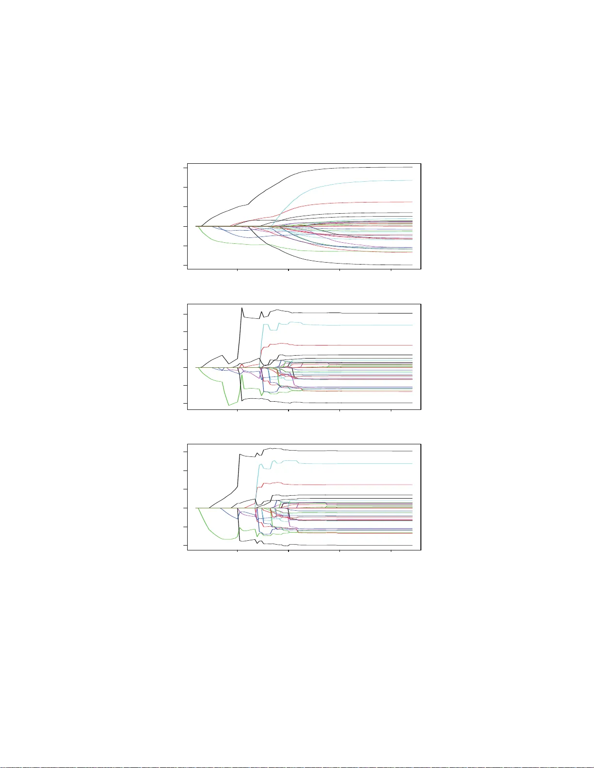
OEM for least squares probl ems Shifeng Xiong 1 , Bin Dai 2 and P eter Z. G . Qian 3 1 Academ y of Mathematics and Systems Science Chinese Academ y of Sciences, Beijing 10019 0 2 T o w er Researc h Capital, 37 7 Broadw a y , New Y or k, NY 10013 3 Departmen t of Sta tistics Univ ersit y of Wisconsin-Madison, Madison, WI 5370 6 Abstract W e prop ose an alg orithm, called OEM (a.k.a. orthogonalizing EM), in tended for v ar- ious least squares problems. The ﬁrst st ep, named activ e orthogonizatio n, orthogonaliz es an arb i- trary regression matrix b y elab orately adding more ro ws. The second step imputes the resp onses of the new ro w s. The third step solv es the least sq u ares p roblem of inte rest for the complete orthog- onal design. The second and third steps ha v e simp le closed forms, and iterate unti l conv ergence. The algorithm works for ordinary least squares and regularized least squares with the lasso, SCAD, MCP and other p enalties. It has sev eral attractiv e theoretic al p r op erties. F or th e ord inary least squares with a singular regression matrix, an OE M sequence con v erges to th e Mo ore-P enrose gen- eralized inv erse-based least s quares estimator. F or the S CAD and MCP , an OEM sequence can ac hieve the oracle prop erty after suﬃcient iterations f or a ﬁxed or dive rging num b er of v ariables. F or ord inary and r egularized least squares w ith v arious p enalties, an O EM sequence con v erges to a p oint ha vin g group ing coherence for fully aliased regression matrices. Con ve rgence and con v ergence rate of the algorithm are examined. These con v ergence rate results sh o w that for the same data set, OEM con v erges faster for regularized least squares th an ordinary least squares. This pro vides a new theoretic al comparison b et ween these metho ds. Numerical examples are pro vided to illustrate the pr op osed algorithm. KEY W ORDS: Design of experimen ts; MCP; Missing data; Optimization; Ora cle prop ert y; Orthogonal design; SCAD; The Lasso. 3 Corresp o nding a uthor: Peter Z . G. Qia n. Email: p eter q @stat.wisc.edu 1 1 INTR ODUCTION Consider a regression mo del y = X β + ε , (1) where X = ( x ij ) is the n × p regression matrix, y ∈ R n is the resp onse vec tor, β = ( β 1 , . . . , β p ) ′ is the v ector of regr ession co eﬃcien ts, and ε is the v ector of random errors with zero mean. The ordinary least squares (OLS) estimator of β is the solution to min β k y − X β k 2 , (2) where k · k denotes t he Euclidean norm. If X is a part of a known m × p orthogonal matrix X c =   X ∆   , (3) where ∆ is a n ( m − n ) × p matrix, (2) can b e eﬃcien tly computed b y the Healy-W estmacott pro cedure ( Healy and W estmacott 19 5 6). Let y c = ( y ′ , y ′ miss ) ′ (4) b e the ve ctor of complete resp onses with missing data y miss of m − n p oints. In eac h iteration, the pro cedure imputes t he v alue of y miss , and up dates the OLS estimator for the complete data ( X c , y c ). This updat e in v olv es no matrix in v ersion since X c is (column) orthogonal. Dempster, Laird, a nd Rubin (1977 ) show ed that this pro cedure is an EM a lg orithm. The ma jor limita t ion of the pro cedure is the assumption that X m ust b e em b edded in a pr e-sp e ciﬁe d orthogonal matrix X c . W e pr o p ose a new algorithm, called ortho gonali z i n g EM (OEM) alg orithm, to remo ve this restriction and extend to o t her directions. The ﬁrst step, called active o rthogonization, orthogonalizes an a r bitr ary regression matrix b y elab o rately adding more rows . The second step imputes the resp onses of the new r o ws. The third step solv es the OLS problem in (2 ) for the complete orthogonal design. The se cond and third 2 steps hav e simple closed forms, and iterate un til con v ergence. F or the OLS pr o blem in (2 ) , OEM w orks with an arbitrary r egr ession matrix X . F or X with no full column rank, the OL S estimator is not unique, a nd w e pro v e that the OEM algorithm con v erges to the Mo ore-Pe nrose generalized in ve rse-based least squares estimator. OEM outp erforms existing metho ds for such an inv erse. OEM also w orks for r e gularize d least squares problems by adding p enalties o r constrain ts to β in (2). These p enalties in clude the ridge regression (Ho erl and Kennard 1970) , the nonnegativ e garrote (Breiman 1995), the lasso (Tibshirani 1996 ) , the SCAD (F an a nd Li 2001), a nd the MCP (Zhang 2 010), amo ng others. Here, the ﬁrst step of OEM uses the same activ e orthog onalization as that for OLS. The second a nd third steps o f OEM imputes t he missing data and solv es the regularized problem f or the complete data ( X c , y c ). Both the second and third steps ha v e a simple closed f orm. W e prov e that OEM con ve rges to a lo cal minim um or stable p oin t o f the regularized least squares problem under mild conditions. Con ve rgence rate o f OEM is also established. These con v ergence rate results sho w that for the same data, OEM conv erges faster for regularized least squares tha n ordinary least squares. This diﬀ erence pro vides a new theoretical comparison b et w een these metho ds. Compared with existing algo rithms, OEM p ossesses tw o unique theoretical features. 1. A chieving the or acle pr op erty for nonc onve x p enalties : An estimator of β in ( 1) having the oracle prop erty can not o nly select the correct submo del asymptotically , but a lso estimate the nonzero co eﬃcien ts as eﬃcien tly as if the correct submo del w ere kno wn in adv ance. F an and Li (2 0 01) prov ed that there exists a lo cal solution of SCAD with this prop erty . F rom the optimization viewpoint, the SCAD problem can ha v e many lo cal minima (Huo and Chen 2010) and it is not clear whic h one has this prop ert y . Zou and Li (2008 ) prop osed the lo cal linear appro ximation (LLA) algo rithm to solve the SCAD problem and show ed that the one-step LLA estimator has the oracle prop erty with a go o d initial estimator for a ﬁxed p . The LLA estimator is not gua ran teed to b e a lo cal minimum of SCAD. T o the b est o f our kno wledge, no theoretical results so far show that an y existing a lgorithm can pro vide suc h a lo cal minim um. W e prov e that the OEM solution f o r SCAD can ac hiev e a lo cal solution with this prop ert y . 2. Havin g gr ouping c oher enc e : An estimator of β is said to ha ve grouping 3 coherence if it ha s the same co eﬃcien t for full aliased columns in X . F or the lasso, SCAD, and MCP , an OEM sequence con v erges to a p oin t ha ving gro uping coherence, whic h implies that the full a liased v ariables will b e in or out of the selected mo del together. This pro p ert y cannot b e a c hiev ed b y exis ting algorithms including the coo r dina t e descen t a lgorithm. In terms of n umerical p erformance, OEM can b e v ery fast for ordinary least squares problems and SCAD for big tall dat a with n > p . F or big wide data with p > n , OEM can b e slo w. This dra wbac k can b e mitigated b y adopting a t wo-stage pro cedure lik e that in F an and Lv (2008), where t he ﬁrst stage uses a screening a pproac h to reduce the dimensionalit y to a mo derate size, and the second stage uses OEM. The remainder of the article will unfo ld as follow s. Section 2 discusses the active or- thogonalization pro cedure. S ection 3 presen ts OEM for OLS. Section 4 extends OEM to regularized least squares. Section 5 provide s con v ergence properties of OEM. Section 6 sho ws that for a regression matrix with full aliased columns, an OEM sequence for the lasso, SCAD, or MCP con ve rges to a solution with gro uping coherency . Section 7 establishes the oracle prop erty of the OEM solution for SCAD and MCP . Section 8 presen ts n umerical examples to compare OEM with other algorithms for regularized least squares. Section 9 concludes with some discuss ion. 2 A CTIVE OR THOGONALIZA TION F or an arbitra r y n × p matrix X in (1), w e prop ose active ortho goliza tion to a ctiv ely orthogolize an arbitrary matrix b y elab orat ely adding more ro ws. Let S b e a p × p diagonal matrix with non- zero diagonal elemen ts s 1 , . . . , s p . Deﬁne Z = X S − 1 . (5) Consider t he eigenv alue decomp osition V ′ Γ V of Z ′ Z (Wilkinson 1965), where V is an orthogonal matrix and Γ is a diagonal matrix whose diagonal elemen ts, γ 1 > · · · > γ p , are 4 the nonnegativ e eigenv alues of Z ′ Z . F or d > γ 1 , let t = # { j : γ j = d, j = 1 , . . . , p } (6) denote the n um b er of the γ j equal d . F o r example, if d = γ 1 = γ 2 and γ 1 > γ j for j = 3 , . . . , p , then t = 2. If d > γ 1 , then t = 0 . Deﬁne B = diag ( d − γ t +1 , . . . , d − γ p ) (7) and ∆ = B 1 / 2 V 1 S , (8) where V 1 is the submatrix of V consisting of t he last p − t r ows. Put X and ∆ row b y row together to fo r m a complete matrix X c . Lemma 1. The matrix X c ab ov e is column ortho g onal. Pr o of. F rom (7) and (8), X ′ c X c = X ′ X + ∆ ′ ∆ = S ( V ′ Γ V + V ′ 1 B V 1 ) S . F or the p × p iden tity matrix I p , d I p − Γ =   0 0 0 B   It then follows that X ′ c X c = S [ V ′ Γ V + V ′ ( d I p − Γ ) V ] S = d S 2 , which completes the pro of. Here is the underlying geometry of activ e orthogolizatio n. F o r a v ector x ∈ R m , let P ω x denote its pro jection on to a subspace ω of R m . Lemma 1 implies that for the column v ectors x 1 , . . . , x p ∈ R n of X in (1), t here exists a set of m utually o rthogonal v ectors x c 1 , . . . , x cp ∈ R n + p − t of X c in (3 ) satisfying P R n x ci = x i , fo r j = 1 , . . . , p . Prop osition 1 mak es t his precis e. 5 y x 2 x c2 z O x c1 x 1 x Figure 1: Expand t w o t w o-dimensional v ectors x 1 and x 2 to t wo three-dimensional v ectors x c1 and x c2 with x ′ c1 x c2 = 0 . Prop osition 1. Let ω b e an n - dimensional subspace of R m with n 6 m . If p 6 m − n + 1 , then for any p vectors x 1 , . . . , x p ∈ ω , there exist p v ectors x c1 , . . . , x c p ∈ R m suc h that P ω x c i = x i for j = 1 , . . . , p and x ′ c i x c j = 0 for i 6 = j . F or illustration, Figure 1 expands t wo v ectors x 1 and x 2 in R 2 to tw o orthogonal ve ctors x c 1 and x c 2 in R 3 . Remark 1. In (8) ∆ has p − t ro ws, whic h do es not rely on the num b er of ro ws in X , and only p − t ro ws need to b e a dded to mak e it ort ho gonal. Remark 2. The form of S in (5) can b e c hosen ﬂexibly . One p ossibilit y is S = I p with X ′ X + ∆ ′ ∆ = d I p (9) with d > γ 1 , and X c is standardized a s the Euclidean norm of eac h column is d . 6 Example 1. Supp o se that X in (1) is orthogo na l. T ak e d = γ 1 and S = diag " ( n X i =1 x 2 i 1 ) 1 / 2 , . . . , ( n X i =1 x 2 ip ) 1 / 2 # . (10) Since t = p , ∆ in (8) is empt y , whic h indicates that activ e orthogonalization will not ov er- sho ot. Example 2. Let X =         0 0 3 / 2 − 4 / 3 − 2 / 3 1 / 6 2 / 3 4 / 3 1 / 6 − 2 / 3 2 / 3 − 7 / 6         . If S = I 3 and d = γ 1 , (8) gives ∆ = ( − 2 / √ 3 , 2 / √ 3 , 1 / √ 3) . Example 3. Consider a t wo-lev el design in three factors         − 1 − 1 − 1 − 1 1 1 1 − 1 1 1 1 − 1         . The regression matrix including all main eﬀects and tw o-w ay in teractions is X =         − 1 − 1 − 1 1 1 1 − 1 1 1 − 1 − 1 1 1 − 1 1 − 1 1 − 1 1 1 − 1 1 − 1 − 1         , where the last three columns for the interactions are fully aliased with the ﬁrst three columns 7 for the main eﬀects. F or S = I 3 and d = γ 1 , (8) gives ∆ =      0 − 2 0 0 − 2 0 0 0 − 2 − 2 0 0 − 2 0 0 0 0 − 2      . The structure of ∆ is ﬂexible in that the interaction columns do not need to b e a pro duct of other tw o columns. Example 4. Consider a 1 000 × 1 0 random matrix X = ( x ij ) with en tries indep enden t ly dra wn from the uniform distribution on [0 , 1). Using S in (1 0 ), (8) giv es ∆ =                        − 7 . 99 16 . 06 − 6 . 39 − 18 . 26 12 . 91 − 8 . 67 7 . 56 34 . 08 − 17 . 04 − 11 . 81 26 . 83 − 12 . 09 7 . 91 1 . 02 − 22 . 75 − 6 . 90 − 19 . 98 26 . 1 0 − 0 . 86 0 . 88 − 4 . 01 1 . 48 9 . 51 − 21 . 99 19 . 46 − 10 . 27 − 25 . 12 − 3 . 39 7 . 29 27 . 90 21 . 77 10 . 72 − 0 . 61 − 6 . 46 28 . 00 1 . 2 8 − 6 . 86 − 7 . 04 11 . 13 − 30 . 64 − 15 . 78 5 . 60 − 15 . 2 6 − 7 . 67 − 9 . 76 23 . 93 − 14 . 71 12 . 25 29 . 45 − 7 . 89 16 . 34 10 . 61 − 41 . 82 11 . 82 6 . 49 − 7 . 38 − 6 . 14 − 1 . 82 − 1 . 86 13 . 09 − 8 . 15 24 . 97 12 . 11 24 . 35 3 . 66 − 2 . 59 − 27 . 84 − 3 . 45 − 9 . 40 − 13 . 72 − 5 . 35 − 21 . 70 − 4 . 16 7 . 42 13 . 98 29 . 84 − 10 . 26 7 . 60 − 25 . 13 7 . 78 − 19 . 62 − 22 . 43 − 2 . 61 22 . 58 11 . 80 − 22 . 08 1 . 25 15 . 87 14 . 94 0 . 31                        . Only nine ro ws need to b e added to mak e this large X matrix orthogonal. 3 OEM F OR ORDINAR Y LEAST SQUARES W e now study OEM fo r the O LS problem in (2 ) when the regression matrix X has an arbitrary form. The ﬁrst step of OEM is activ e orthogonalizatio n to obtain ∆ in (8). F o r an initial estimator β (0) , the second step imputes y miss in (4) by y I = ∆ β (0) . Let y c = ( y ′ , y ′ I ) ′ . 8 The third step solv es β (1) = a rgmin β k y c − X c β k 2 . (11) Then, the second and third steps iterate for obtaining β (2) , β (3) , . . . un til conv ergence. Deﬁne A = ∆ ′ ∆ . (12) F or X c in (3), let ( d 1 , . . . , d p ) denote the diagonal elemen ts of X ′ c X c . F or k = 0 , 1 , . . . , let u = ( u 1 , . . . , u p ) ′ = X ′ y + A β ( k ) , (13) and (11) b ecomes β ( k +1) = arg min β p X j =1 ( d j β 2 j − 2 u j β j ) , (14) whic h is sep ar able in the dimensions of β . Th us, (14) has a simple form β ( k +1) j = u j /d j , for j = 1 , . . . , p, (15) whic h in volv es no matrix inv ersion. In (13), for activ e orthogonalization, instead of computing ∆ in (8), one can compute A = ∆ ′ ∆ and the diagonal en tries d 1 , . . . , d p of X ′ c X c . If S = I p in (8), A = d I p − X ′ X , where d is a n umber no less than the largest eigen v alue γ 1 of X ′ X . A p ossible c hoice is d = trace( X ′ X ). Another c hoice is d = γ 1 to obtain the fastest conv ergence; see Remark 5. W e compute γ 1 b y the p o wer metho d (Wilkinson 1965) describ ed b elo w. Giv en a nonzero initial v ector a (0) ∈ R p , let γ (0) 1 = k a (0) k . F or k = 0 , 1 , ... , compute a ( k +1) = X ′ X a ( k ) /γ ( k ) 1 and γ ( k +1) 1 = k a ( k +1) k until con v ergence. If a (0) is not an eigenv ector of an y γ j unequal to γ 1 , then γ ( k ) 1 con verges to γ 1 . F o r t in (6), the conv ergence rate of the p o we r metho d is linear (W atkins 2 0 02) sp eciﬁed b y lim k →∞ k γ ( k +1) 1 − γ 1 k k γ ( k ) 1 − γ 1 k = γ t +1 γ 1 . 9 When p > n , r eplace the p × p matrix X ′ X with the n × n matrix X X ′ in the p ow er metho d to reduce computational cost as the t wo matr ices ha v e the same non-zero eigen v alues. When X has full column rank, the con ve rgence results in W u (1983 ) indicates that the OEM sequence given by (15) conv erges t o the OLS estimator f or an y initial p oin t β (0) . Next, w e discuss the conv ergence pro p ert y of OEM when X ′ X is singular, whic h co v ers the case of p > n . Let r denote the rank of X . F or r < p , the singular v alue decomp osition (Wilkinson 1965) of X is X = U ′   Γ 1 / 2 0 0 0 0   V , where U is an n × n orthogonal matrix, V is a p × p ort ho gonal matrix, and Γ 0 is a diagonal matrix with diagonal elemen ts γ 1 > · · · > γ r whic h are the p ositiv e eigenv alues of X ′ X . Deﬁne ˆ β ∗ = ( X ′ X ) + X ′ y , (16) where + denotes the Mo ore-P enrose generalized inv erse (Ben-Israel and Greville 2003 ). Theorem 1. Supp ose that X ′ X + ∆ ′ ∆ = γ 1 I p . If β (0) lies in the linear space spanned b y the ﬁrst r columns of V ′ , then as k → ∞ , for the OEM sequence { β ( k ) } of the ordinary least squares, β ( k ) → ˆ β ∗ . Pr o of. Deﬁne D = I p − γ − 1 1 X ′ X . No te that β ( k +1) = γ − 1 1 X ′ y + D β ( k ) . By induction, β ( k ) = γ − 1 1 ( I p + D + · · · + D k − 1 ) X ′ y + D k β (0) = γ − 1 1 V ′    I p +   I r − γ − 1 1 Γ 0 0 0 − I p − r   + · · · +   ( I r − γ − 1 1 Γ 0 ) k − 1 0 0 ( − 1) k − 1 I p − r      · V V ′   Γ 1 / 2 0 0 0 0   U y + D k β (0) = γ − 1 1 V ′    I r + ( I r − γ − 1 1 Γ 0 ) + · · · + ( I r − γ − 1 1 Γ 0 ) k − 1  Γ 1 / 2 0 0 0 0   U y + D k β (0) . 10 As k → ∞ , D k → V ′   0 I p − r   V and D k β (0) → 0, whic h implies that β ( k ) → V ′   Γ − 1 / 2 0 0 0 0   U y = ˆ β ∗ . This completes the pro of. In active orthogona lization, t he condition X ′ X + ∆ ′ ∆ = γ 1 I p holds if d = γ 1 and S = I p in (8). Using β (0) = 0 satisﬁes the condition in Theorem 1. The Mo ore-Pe nrose generalized inv erse is widely used in statistics for a dege nerated system. Theorem 1 indicates that OEM conv erges to ˆ β ∗ in (16) in this case. When r < p , the limiting v ector ˆ β ∗ giv en by an OEM sequence has the follo wing prop erties. First, it has the minimal Euclidean nor m among the least squares estimators ( X ′ X ) − X ′ y ( Ben-Israel and Greville 2003). Second, its mo del error has a simple form, E  ( ˆ β ∗ − β ) ′ ( X ′ X )( ˆ β ∗ − β )  = r σ 2 . Third, X α = 0 implies α ′ ˆ β ∗ = 0 for an y ve ctor α . The third prop erty indicates that ˆ β ∗ inherits the multic ollinearit y b et w een the columns in X . This prop erty is strong er than grouping coherence for regularized least squares in Section 6. A widely used metho d for computing ˆ β ∗ is to obtain ( X ′ X ) + b y the eigenv alue decomp o- sition (Golub a nd V an Lo an 1 996) and then compute the pro duct of ( X ′ X ) + and X ′ y . This metho d is implemen ted in the MATLAB function pinv with core co de in Fortran and in the R function ginv with core co de in C++ . The R function is slo w er than the MATLAB function. When some eigenv alues are close to zero, the eigen v alue decompo sition metho d is unstable, and OEM is more stable due to its it era t ive nature. The following example illustrates t his diﬀerence. Example 5. Construct a 10 × 4 matrix X =  diag (1 , 1 , 1 , √ u ) 0  ′ , where u is generated from a unifo r m distribution on [10 − 16 , 10 − 14 ). T he eigen v alues of X ′ X are 1 , 1 , 1, and u . Generate all en tries of y indep enden tly fr o m the uniform distribution on [0 , 1). W e compare 11 OEM and the eigenv alue decomposition metho d for computing ˆ β ∗ using the MATLAB function pinv . F or OEM, the stopping criterion is whe n relative changes in all co eﬃcien ts are less than 10 − 4 . The tw o metho ds are replicated 100 times in MATLAB . Ov er the 10 0 r eplicates, the largest a nd smallest v alues of k ˆ β ∗ k by the eigen v alue decomp osition metho d are 2 . 06 × 1 0 7 and 0 . 2 5, indicating unstability . The t w o v alues computed by OEM are 1 . 48 and 0 . 25, whic h are m uc h more stable. Next, w e discuss the computational eﬃciency of O EM for computing ˆ β ∗ in (16) when X is degenerated. Recall that X ′ X and X X ′ ha ve t he same no nzero eigen v alues. The computa- tion of γ 1 in the OEM itera t io ns b y the p o w er metho d has complexit y O  min { n, p } 2 max { n, p }  . Since the complexit y of the OEM iterations is O ( np 2 ), the whole computational complex- it y of OEM for computing ˆ β ∗ is O ( np 2 ). T he eigen v alue decomp osition metho d computes ( X ′ X ) + ﬁrst b y eigen v alue decomp o sition to obtain ˆ β ∗ , and has computational complexit y O ( np 2 + p 3 ). The OEM a lgorithm is sup erio r to this metho d in terms o f complexit y . n p OEM eigen v alue decomp osition 50 , 000 10 0 . 0 433 0 . 0956 50 0 . 2 439 0 . 4098 200 1 . 4156 4 . 9765 1000 5 . 4165 45 . 3270 5 , 000 72 . 0630 442 . 3300 T able 1: Av erage runtime (second) comparison b et w een OEM and the prev ailing metho d for n > p W e conduct a simulation study to compare the sp eeds of OEM and the eigen v alue decom- p osition metho d for computing ˆ β ∗ in (16). Generate all en tries of X and y indep endently from the standard normal distribution. A new predictor calculated as the mean o f all the co v ariat es is added to degenerate the des ign matrix. T ables 1 a nd 2 compare our R pac k- age oem with main co de in C++ and the eigen v alue decomp osition metho d in computing ˆ β ∗ . The tw o metho ds giv e the same results. T ables 1 and 2 indicate that OEM is faster than the eigenv alue decomp osition metho d for an y combination of n and p , v alidating the ab ov e 12 p n OEM eigen v alue decomp osition 50 , 000 10 0 . 0482 0 . 1153 50 0 . 4203 0 . 4176 200 1 . 9159 5 . 2053 1000 8 . 4626 47 . 76 5 3 5 , 000 71 . 8477 440 . 6741 T able 2: Av erage run time (second) comparison b et we en OEM and the eigen v alue decomp o- sition metho d for p > n complexit y analysis. 4 OEM F OR REGULARIZED LEAST SQUA RES It is easy to extend OEM to regularized least squares problems. Consider a penalized v ersion of (1): min β ∈ Θ  k y − X β k 2 + P ( β ; λ )  , (17) where β ∈ Θ, Θ is a subset of R p , P is a p enalt y function, and λ is the v ector of tuning parameters. T o apply the p enalt y P equally to all the v ariables, the regression matr ix X is standardized so that n X i =1 x 2 ij = 1 , for j = 1 , . . . , p. (18) P opular choices for P include the r idg e regression (Ho erl and Kennard 1970), the nonnegat iv e garrote (Breiman 1995), the la sso (Tibshirani 1996), the SCAD (F an a nd Li 2001) , and the MCP (Zhang 20 10). Supp ose that Θ and P in (17) a re de c omp o s able a s Θ = Q p j =1 Θ j and P ( β ; λ ) = P p j =1 P j ( β j ; λ ). F o r the problem in (17), the ﬁrst step of OEM is active o rthogonaliza- tion, whic h computes ∆ in (8). F or an initial estimator β (0) , t he second step imputes y miss 13 in (4) by y I = ∆ β (0) . Let y c = ( y ′ , y ′ I ) ′ . The third step solv es β (1) = arg min β ∈ Θ  k y c − X c β k 2 + P ( β ; λ )  . The second and third steps it erate to compute β ( k ) for k = 1 , 2 , . . . un til conv ergence. Similar to (14), w e hav e a n iterativ e formula β ( k +1) j = arg min β j ∈ Θ j  d j β 2 j − 2 u j β j + P j ( β j ; λ )  , for j = 1 , . . . , p, (19) with u = ( u 1 , . . . , u p ) ′ in (13). This shortcut applies to the follow ing p enalties: 1. The lasso (Tibshirani 1996), where Θ j = R , P j ( β j ; λ ) = 2 λ | β j | , (20) and (19) b ecomes β ( k +1) j = sign( u j )  | u j | − λ d j  + . (21) Here, for a ∈ R , ( a ) + denotes max { a, 0 } . 2. The nonnegativ e garrot e (Breiman 1995), where Θ j = { x : x ˆ β j > 0 } , P j ( β j ; λ ) = 2 λβ j / ˆ β j , ˆ β j is the OLS estimator of β j , and (19) b ecomes β ( k +1) j = u j ˆ β j − λ d j ˆ β 2 j ! + ˆ β j . 3. The elastic-net (Zou and Hastie 20 0 5), where Θ j = R , P j ( β j ; λ ) = 2 λ 1 | β j | + λ 2 β 2 j . (22) and (19) b ecomes β ( k +1) j = sign( u j )  | u j | − λ 1 d j + λ 2  + . (23) 14 5. The SCAD (F an and Li 2001 ) , where Θ j = R , P j ( β j ; λ ) = 2 P λ ( | β j | ), and P ′ λ ( θ ) = λI ( θ 6 λ ) + ( aλ − θ ) + I ( θ > λ ) / ( a − 1) , (24) with a > 2, λ > 0, and θ > 0. Here, I is the indicator function. If X in (1) is standardized as in (1 8 ) with d j > 1 f o r all j , (19) b ecomes β ( k +1) j =          sign( u j )  | u j | − λ  + /d j , when | u j | 6 ( d j + 1) λ, sign( u j )  ( a − 1) | u j | − aλ  /  ( a − 1) d j − 1  , when ( d j + 1) λ < | u j | 6 aλd j , u j /d j , when | u j | > aλd j . (25) 6. The MCP (Zha ng 2010), where Θ j = R , P j ( β j ; λ ) = 2 P λ ( | β j | ), and P ′ λ ( θ ) = ( λ − θ /a ) I ( θ 6 aλ ) (26) with a > 1 and θ > 0. If X in (1) is standardized as in (18 ) with d j > 1 for all j , (19) b ecomes β ( k +1) j =    sign( u j ) a  | u j | − λ  + / ( ad j − 1) , when | u j | 6 aλd j , u j /d j , when | u j | > aλd j . (27) 7. The “Berh u” p enalty ( O w en 2006), where Θ j = R , P j ( β j ; λ ) = 2 λ  | β j | I ( | β j | < δ ) + ( β 2 j + δ 2 ) I ( | β j | > δ ) / (2 δ )  for some δ > 0, and (19) b ecomes β ( k +1) j =    sign( u j )  | u j | − λ  + /d j , when | u j | < λ + d j δ , u j δ / ( λ + d j δ ) , when | u j | > λ + d j δ . OEM for (17) is an EM algorithm. Let the o bserv ed data y follo w the mo del in (1). Assume that the complete data y c = ( y ′ , y ′ miss ) ′ in ( 4 ) follows a regression mo del y c = X c β + ε c , where ε c is from N ( 0 , I m ). Let ˆ β b e a solution to (17) giv en by ˆ β = argmax β ∈ Θ L ( β | y ), 15 and the regular ized lik eliho o d function L ( β | y ) is (2 π ) − n/ 2 exp  − 1 2 k y − X β k 2  exp  − 1 2 P ( β ; λ )  . Giv en β ( k ) , the second step of OEM for (17 ) is the E-step, E  log { L ( β | y c ) } | y , β ( k )  = − C  k y − X β k 2 + E  k y miss − X β k 2 | β ( k )  + P ( β ; λ )  = − C  n + k y − X β k 2 + k ∆ β ( k ) − ∆ β k 2 + P ( β ; λ )  for some constan t C > 0. D eﬁne Q ( β | β ( k ) ) = k y − X β k 2 + k ∆ β ( k ) − ∆ β k 2 + P ( β ; λ ) . (28) The third step of OEM is the M-step, β ( k +1) = a rg min β ∈ Θ Q ( β | β ( k ) ) , (29) whic h is equiv alen t to (19) when Θ and P in (17) are decomp o sable. Example 6. F or the mo del in (1), let the complete matrix X c b e an o rthogonal design from Xu (2 009) with 4096 runs in 30 fa ctors. Let X in (1) b e the submatrix of X c consisting of the ﬁrst 300 0 ro ws and let y b e generated from (1) with σ = 1 and β j = ( − 1) j exp  − 2( j − 1) / 20  for j = 1 , . . . , p. (30) Here, let p = 30, n = 3000, and the resp onse v alues for the last 1096 r ows of X c b e missing. OEM is used to solv e the SCAD problem with an initial v alue β (0) = 0 and a stopping criterion when relativ e c hanges in all co eﬃcien ts are less than 10 − 6 . F or λ = 1 a nd a = 3 . 7 in (24), Figure 2 plots v alues of the ob j ective function in (17) with the SCAD p enalt y of the OEM sequence against iteration n umbers, where the con ve rgence o ccurs at iterat io n 13, and 16 0 2 4 6 8 10 12 2775 2780 2785 2790 2795 2800 2805 2810 iteration Figure 2: V alues of the ob jectiv e function of an OEM sequence for the SCAD against itera- tions for Example 6. the ob jectiv e function signiﬁcan tly reduces af ter t wo iterations. 5 CONVER GENCE OF THE OEM ALGORITHM W e now deriv e con vergenc e prop erties o f OEM with the general p enalt y in (17). W e also give results to compare the con vergenc e ra t es of OEM for OLS, the elastic-net, and the lasso. These conv ergence rate results show that for the same data set, O EM con ve rges faster for regularized least squares than ordinary least squares. This pro vides a new theoretical comparison b etw een these metho ds. The ob jectiv e functions of existing EM con v ergence results lik e those in W u (1983), Green (1 990) and McLac hlan and K rishnan (2008) are t ypically con tinuously diﬀeren tia ble. This condition do es not hold for the o b j ective function in ( 1 7) with the lasso and other p enalties, and these existing results do not directly apply here. W e mak e sev eral assumptions for Θ and P ( β ; λ ) in (17). Assumption 1. The parameter space Θ is a closed conv ex subset of R p . Assumption 2. F or a ﬁxed λ , the p enalty P ( β ; λ ) → + ∞ as k β k → + ∞ . Assumption 3. F or a ﬁxed λ , the p enalty P ( β ; λ ) is con tin uous with r esp ect to β ∈ Θ. 17 All p enalties discussed in Section 4 satisfy these assumptions. The assum ptions co v er the case in whic h the iterativ e se quence { β ( k ) } deﬁned in (29) ma y fall on the b oundary of Θ (Nettleton 1999), lik e the nonnegative ga rrote (Breiman 1995) and the nonnegativ e lasso (Efron et al. 2004). The bridge p enalt y (F rank and F riedman 1993) in (33) also satisﬁes the ab ov e assumptions. F or the mo del in (1), denote the ob jectiv e function in (17) by l ( β ) = k y − X β k 2 + P ( β ; λ ) . (31) F or p enalties lik e the bridge, it is infeasible to p erform the M-step in (29) directly . F or this situation, following the generalized EM algorithm in D empster, Laird, and Rubin (1977 ), we deﬁne the fo llo wing gener alize d OEM algorithm β ( k ) → β ( k +1) ∈ M ( β ( k ) ) , (32) where β → M ( β ) ⊂ Θ is a p oin t- to-set map suc h that Q ( φ | β ) 6 Q ( β | β ) , for all φ ∈ M ( β ) . Here, Q is g iv en in (28). The OEM sequence deﬁned by (29) is a sp ecial case of (3 2). F or example, the generalized OEM algorithm can b e used for t he bridge p enalt y , where Θ j = R and P j ( β j ; λ ) = λ | β j | a (33) for some a ∈ (0 , 1) in (1 7). Since t he solution to (19) with the bridge p enalty has no closed form, one ma y use one-dimensional searc h to compute β ( k +1) j that satisﬁes (32) . By Assumption 1, { β ∈ Θ : l ( β ) 6 l ( β (0) ) } is compact for any l ( β (0) ) > −∞ . By Assumption 3, M is a closed p oint-to-set ma p (Zangwill 1969; W u 1983). The ob jectiv e functions in (17) with the lasso and other p enalties are not con tin uously diﬀeren tiable. A mor e general deﬁnition of stationa ry po in ts is neede d. W e call β ∈ Θ a 18 stationary p o in t of l if lim inf t → 0 + l  (1 − t ) β + t φ  − l ( β ) t > 0 for all φ ∈ Θ . Let S denote the set of stationary p oints of l . Analogous to Theorem 1 in W u (1983) o n the global con v ergence of the EM algorithm, w e hav e the follo wing result. Theorem 2. Let { β ( k ) } b e a generalized OEM sequence generated b y (32). Supp ose that l ( β ( k +1) ) < l ( β ( k ) ) for all β ( k ) ∈ Θ \ S. (34) Then all limit p oints of { β ( k ) } are elemen ts of S and l ( β ( k ) ) conv erges monotonically to l ∗ = l ( β ∗ ) for some β ∗ ∈ S . Theorem 3. If β ∗ is a lo cal minim um of Q ( β | β ∗ ), then β ∗ ∈ S . This theorem fo llows from the fact tha t l ( β ) − Q ( β | β ∗ ) is diﬀeren t ia ble and ∂  l ( β ) − Q ( β | β ∗ )  ∂ β    β = β ∗ = 0 . Remark 3. By Theorem 3, if β ( k ) / ∈ S , then β ( k ) cannot b e a lo cal minim um of Q ( β | β ( k ) ). Th us, there exists at least one p oint β ( k +1) ∈ M ( β ( k ) ) suc h t ha t Q ( β ( k +1) | β ( k ) ) < Q ( β ( k ) | β ( k ) ) and therefore satisﬁes the condition in (3 4). As a sp ecial case, a n O EM sequence generated b y (29) satisﬁes (34) in Theorem 2. Next, we deriv e conv ergence r esults of a generalized OEM sequence { β ( k ) } in (32), whic h, b y Theorem 3, hold automatically for an OEM se quence. If the p enalty function P ( β ; λ ) is con v ex and l ( β ) has a unique minim um, Theorem 4 sho ws that { β ( k ) } con verges to the global minim um. Theorem 4. F or { β ( k ) } deﬁned in Theorem 2, supp o se t ha t l ( β ) in (31) is a con vex function on Θ with a unique minim um β ∗ and tha t (34) holds for { β ( k ) } . Then β ( k ) → β ∗ as k → ∞ . 19 Pr o of. It suﬃces to sho w that S = { β ∗ } . F or φ ∈ Θ with φ 6 = β ∗ and t > 0, l  (1 − t ) φ + t β ∗  − l ( β ∗ ) t 6 tl ( β ∗ ) + (1 − t ) l ( φ ) − l ( φ ) t = l ( β ∗ ) − l ( φ ) < 0 . This implies φ / ∈ S . Theorem 5 discusses the con v ergence o f an OEM sequence { β ( k ) } for more general p enal- ties. F or a ∈ R , deﬁne S ( a ) = { φ ∈ S : l ( φ ) = a } . F rom Theorem 2, all limit p oin ts of an OEM sequence are in S ( l ∗ ), where l ∗ is the limit of l ( β ( k ) ) in Theorem 2 . Theorem 5 states that the limit p o in t is unique under certain conditions. Theorem 5. Let { β ( k ) } b e a g eneralized OEM sequence generated by (32) with ∆ ′ ∆ > 0. If (34 ) holds, then all limit p oints of { β ( k ) } ar e in a connected and compact subset of S ( l ∗ ). In particular, if the set S ( l ∗ ) is discrete in that its only connecte d comp onen ts are singletons, then β ( k ) con verges to some β ∗ in S ( l ∗ ) as k → ∞ . Pr o of. Note that Q ( β ( k +1) | β ( k ) ) = l ( β ( k +1) ) + k ∆ β ( k +1) − ∆ β ( k ) k 2 6 Q ( β ( k ) | β ( k ) ) = l ( β ( k ) ). By Theorem 2, k ∆ β ( k +1) − ∆ β ( k ) k 2 6 l ( β ( k ) ) − l ( β ( k +1) ) → 0 as k → ∞ . Th us, k β ( k +1) − β ( k ) k → 0 . This theorem now follo ws immediately from Theorem 5 o f W u (1 983). Since t he bridge, SCAD and MCP p enalties all satisfy the condition that S ( l ∗ ) is discrete, an OEM sequence for any of them con v erges to the statio na ry p oints of l . Theorem 5 is obtained under the condition ∆ ′ ∆ is not singular. It is easy to sho w that Theorem 5 holds with probability one if the error ε in (1) has a con tinuous distribution. W e now deriv e the conv ergence rate of the OEM sequence in (29). F o llo wing Dempster, Laird, and Rubin (1977), write β ( k +1) = M ( β ( k ) ) , where the map M ( β ) = ( M 1 ( β ) , . . . , M p ( β )) ′ is deﬁned by (29). W e captur e the con v ergence rate of t he OEM sequence { β ( k ) } through M . Assume that (9 ) holds f or d > γ 1 , where γ 1 20 is the largest eigen v alue of X ′ X . F o r activ e o r t hogolization in Section 2, this assumption holds b y taking S = I p ; see R emark 2. Let β ∗ b e the limit of the OEM sequence { β ( k ) } . As in Meng (1994), w e call R = lim sup k →∞ k β ( k +1) − β ∗ k k β ( k ) − β ∗ k = lim sup k →∞ k M ( β ( k ) ) − M ( β ∗ ) k k β ( k ) − β ∗ k , (35) the global rate of con ve rgence f o r the OEM se quence. If there is no p enalt y in (17), i.e., computing the OLS estimator, the global r a te of con vergenc e R in (35) b ecomes the largest eigen v alue of J ( β ∗ ), denoted b y R 0 , where J ( φ ) is the p × p Jacobian matrix for M ( φ ) ha ving ( i, j )th entry ∂ M i ( φ ) /∂ φ j . If (9) holds, then J ( β ∗ ) = A /d with A = ∆ ′ ∆ . Th us, R 0 = d − γ p d . (36) F or (17), the p enalty function P ( β ; λ ) typically is not suﬃcien t ly smo oth and R in (35) has no analytic form. Theorem 6 giv es an upp er b ound of R net , the v alue of R fo r the elastic-net p enalt y in (22) with λ 1 , λ 2 > 0. Theorem 6. F or ∆ fr o m (3), if (9) holds, then R NET 6 R 0 . Pr o of. Let x j denote the j th column of n × p matrix X in ( 1) and a j denote the j th column of A = ∆ ′ ∆ , resp ectiv ely . F or an OEM sequence for the elastic-net, b y (23), M j ( β ) = f ( x ′ j y + a ′ j β ) , for j = 1 , . . . , p, where f ( u ) = sign ( u )  | u | − λ 1 d + λ 2  + . 21 F or j = 1 , . . . , p , observ e that | M j ( β ( k ) ) − M j ( β ∗ ) | k β ( k ) − β ∗ k = | f ( x ′ j y + a ′ j β ( k ) ) − f ( x ′ j y + a ′ j β ∗ ) | | ( x ′ j y + a ′ j β ( k ) ) − ( x ′ j y + a ′ j β ∗ ) | · | ( x ′ j y + a ′ j β ( k ) ) − ( x ′ j y + a ′ j β ∗ ) | k β ( k ) − β ∗ k 6 1 d · | a ′ j ( β ( k ) − β ∗ ) | k β ( k ) − β ∗ k . Th us, k M ( β ( k ) ) − M ( β ∗ ) k k β ( k ) − β ∗ k 6 1 d · k A ( β ( k ) − β ∗ ) k k β ( k ) − β ∗ k 6 d − γ p d . This completes the pro of. Remark 4. Theorem 6 indicates that, f or the same X and y in (1 ), the OEM solution for the elastic-net n umerically conv erges faster than its coun terpart for the OLS. Since t he lasso is a sp ecial case of the elastic-net with λ 2 = 0 in ( 22), this theorem holds for the lasso as w ell. Remark 5. F rom (36) a nd Theorem 6, the con vergenc e rate of the OEM algorithm depends on the ratio of γ p and d equal to or la r ger than γ 1 . This rate is t he fastest when d = γ 1 = γ p , i.e., if X is o rthogonal a nd standardized. This result suggests that O EM conv erges faster if X has controlled corr elation like fro m a sup ersaturated design or a nearly orthog o nal La tin h yp ercub e design ( Ow en 1994). Example 7. W e generate X from p dimensional G aussian distribution N ( 0 , V ) with n indep enden t observ ations, where the ( i, j )th en try of V is 1 for i = j and ρ for i 6 = j . V alues of y a nd β are generated by ( 1) and ( 3 0). The same setup w as used in F riedman, Hastie, and Tibshirani (200 9). F or p = 10 , ρ = 0 . 1 , λ = 0 . 5 and increasing n , t he left panel of F igure 3 depicts the av erage v alues of R 0 in (36 ) a gainst increasing n and the righ t panel of the ﬁgure depicts the a verage iteration n um b ers against increasing n , with t he dashed a nd solid lines corresp onding to the OLS estimator and the lasso, resp ectiv ely . This ﬁg ure indicates that OEM requires fewer iterations as n b ecomes larg er, whic h mak es O EM particulary attractive 22 50 100 150 200 0.65 0.7 0.75 0.8 0.85 0.9 0.95 n 50 100 150 200 20 40 60 80 100 120 140 n Figure 3 : (Left) the av erage v alues of R 0 in (36) against increasing n for Example 7; (righ t) the av erage iteration n umbers against increasing n for Example 7 , where the dashed and solid lines denote the OLS estimator and the lasso, r espective ly . for situations with big tall data. Th e OEM seq uence for the lasso requires few er iteration than its counterpart for the OLS, th us v alidating Theorem 6. 6 POSSESSING GR OUPING COHERENCE Data with fully aliasing structures commonly app ear in observ ational studies and de- signed exp erimen ts. Here w e consider the con v ergence of the OEM algorithm when the regression matrix X in (1) is singular due to fully aliased columns. Let X b e standardized as in (18) with columns x 1 , . . . , x p . If x i and x j are fully a liased, i.e., | x i | = | x j | , then the ob jectiv e function in (17) for the lasso is not strictly con vex and has man y minima (Zou and Hastie 2005). If some columns of X a r e iden tical, it is desirable to hav e grouping coherence with the same regression co eﬃcien t. This is suggested b y Zou a nd Hastie (20 0 5) and others. Deﬁnition 1 makes this precise. Deﬁnition 1. An estimator ˆ β = ( ˆ β 1 , . . . , ˆ β p ) ′ of β in (1) has gr ouping c oher enc e if x i = x j implies ˆ β i = ˆ β j and x i = − x j implies ˆ β i = − ˆ β j . Some p enalties other than the lasso can pro duce estimators with grouping coherence (Zou and Hastie 2005 ; Bondell and Reic h 2008; T utz and Ulbrich t 2009; P etry and T utz 2012), but they require more than one tuning par a meters, whic h leads to more computational burden. 23 Inste ad of changing the p enalty, OEM c a n give a lasso so l ution with this pr op erty . This also holds for SCAD and MCP . Recall that ˆ β ∗ in ( 1 6), whic h can be obtained b y OEM, has a stronger prop erty than grouping coherence. Let 0 p denote the zero v ector in R p . Let e + ij b e the v ector obta ined by replacing the i th and j th en tr ies of 0 p with 1. Let e − ij b e the v ector obtained b y replacing the i th a nd j th en tries of 0 p with 1 and − 1, resp ectiv ely . Let E denote the set of all e + ij and e − ij . By D eﬁnition 1, an estimator ˆ β has gro uping coherence if and only if fo r any α ∈ E with X α = 0 , α ′ ˆ β = 0. Lemma 2. Supp ose that (9) holds. F or the OEM sequence { β ( k ) } of the lasso, SCAD or MCP , if X α = 0 and α ′ β ( k ) = 0 for α ∈ E , then α ′ β ( k +1) = 0 . Pr o of. F or u in (13 ) , α ′ u = α ′ X ′ y + α ′ ( d I p − X ′ X ) β ( k ) = 0 for any α ∈ E with X α = 0 and α ′ β ( k ) = 0. Then b y (21), (2 5) and (27), a n OEM seque nce o f the la sso, SCAD or MCP satisﬁes the condition that if α ′ u = 0, then α ′ β ( k +1) = 0 for α ∈ E . This completes the pro of. Remark 6. Lemma 2 implies that, for k = 1 , 2 , . . . , β ( k ) has grouping coherence if β (0) has grouping coherence . Th us, if { β ( k ) } con v erges, then its limit has grouping coherence. By Theorem 5, if d > λ 1 in (9), then an OEM sequence for the SCAD or MCP conv erges t o a p oin t with g r o uping coherence. When X in (1 ) has fully alia sed columns, the ob jectiv e function in (17) for the lasso has man y minima and hence the condition in Theorem 4 do es not hold. Theorem 7 show s that, ev en with full aliasing, an O EM seque nce (21) for the la sso conv erges to a p oint with grouping coherence. Theorem 7. Supp ose that (9) holds. If β (0) has grouping coherence, then as k → ∞ , the OEM sequence { β ( k ) } of the lasso conv erges to a limit that has grouping coherence. Pr o of. P a r t ition columns of X in (1) as ( X 1 X 2 ), whe re no t w o columns of X 2 are fully aliased and an y column of X 1 is fully aliased with at least one column of X 2 . Let J denote the num b er of columns in X 1 . Partition β as ( β ′ 1 , β ′ 2 ) ′ and β ( k ) as ( β ( k ) ′ 1 , β ( k ) ′ 2 ) ′ , 24 corresp onding to X 1 and X 2 , resp ectiv ely . F or j = 1 , . . . , p , let ω ( j ) = # { i = 1 , . . . , p : | x i | = | x j |} . By Lemma 2, for j = 1 , . . . , J , β ( k ) j = β ( k ) j ′ if x j = x j ′ and β ( k ) j = − β ( k ) j ′ otherwise, where j ′ ∈ { J + 1 , . . . , p } . It follows that { β ( k ) 2 } is an O EM seque nce for solving min θ k y − ˜ X θ k 2 + 2 p − J X j =1 | θ j | , (37) where θ = ( θ 1 , . . . , θ p − J ) ′ , and the columns of ˜ X are ω ( J + 1) x J +1 , . . . , ω ( p ) x p . Because the ob jectiv e function in (37) is strictly con v ex, b y Theorem 4 , { β ( k ) 2 } con verges to a limit with grouping coherence. This completes t he pro of. 7 A CHIEVING THE ORA CLE PR OPER TY W ITH NONCONVEX PENAL TIES F an and Li (2001) in tro duced an imp ort a n t concept called the oracle prop erty and sho w ed that there exists one lo cal minimu m of t he SCAD pr o blem with this prop erty when p is ﬁxed. The corr esp o nding results with a div erg ing p we re presen ted in F an and P eng (2004) and F an and Lv (20 1 1). Because the optimization pro blem in (1 7) with t he SCAD p enalt y has an exp o nen tial n um b er of lo cal o ptima (Huo a nd Ni 2007; Huo a nd Chen 2010), no theoretical results in the curren t literature, as far as we are aw are, show that an existing algorithm can pro vide suc h a lo cal minim um. Zou and Li (200 8) prop osed the lo cal linear appro ximation (LLA) algorithm to solve t he SCAD problem and sho we d that the one-step LLA estimator has the or a cle prop erty with a go o d initial estimator fo r a ﬁxed p . The LLA estimator is not guaran teed to b e a lo cal minimum of SCAD. In con trast, w e prov e that the OEM solution to t he SCAD o r MCP can ach iev e this prop ert y . Lik e F an and Pe ng (2004) and F an and Lv (2011), we allow p to dep end on n , whic h co vers the ﬁxed p case as a sp ecial case. 25 Supp ose t ha t the n umber of nonzero co eﬃcien ts of β in (1) is p 1 (with p 1 6 p ) and partition β a s β = ( β ′ 1 , β ′ 2 ) ′ , (38) where β 2 = 0 and no comp onent of β 1 is zero. Divide columns of the regression matrix X in (1) to ( X 1 X 2 ) with X 1 corresp onding to β 1 . A regularized least squares estimator of β in (1 ) has the or a cle prop ert y if it can not only select the correct submodel asymptotically , but also estimate the nonzero co eﬃcien ts β 1 in (38) as eﬃcien tly as if the correct submo del w ere kno wn in a dv ance. Sp eciﬁcally , a n estimator ˆ β = ( ˆ β ′ 1 , ˆ β ′ 2 ) ′ has this prop erty if P( ˆ β 2 = 0 ) → 1 and ˆ β 1 − β 1 follo ws a normal distribution N ( 0 , σ 2 ( X ′ 1 X 1 ) − 1 ) asymptotically . W e now consider the oracle prop erty of OEM sequences for SCAD. First w e prov e that, under certain conditions, a ﬁxed p oint of the OEM iterations for SCAD can p o ssess the oracle prop erty . Here in after, p dep ends o n n but p 1 and β 1 are ﬁxed for simplicit y . A deﬁnition and sev eral assumptions are needed. Deﬁnition 2. F or a series of n umbers c n → ∞ and a p o sitiv e constant κ , an estimator ˆ β of β is said to b e c n -concen trat iv ely consisten t of order κ to β if as n → ∞ , ( i) k ˆ β − β k = O p ( c − 1 n ); (ii) P( c n k ˆ β − β k > h n ) = O (exp( − δ h κ n )) for any h n → + ∞ , where δ > 0 is a constan t. Assumption 4. The random error ε fo llo ws a normal distribution N ( 0 , σ 2 I n ). Assumption 5. The matrix X / √ n is standardized suc h that eac h en t r y on the diagonal of X ′ X /n is 1, and X ′ X /n + ∆ ′ ∆ = d n I p with d n > γ 1 , where γ 1 is the lar gest eigen v alue of X ′ X /n . In active orthog o nalization, d n in Assumption 5 can take an y num b er equal to or larger than γ 1 . Assumption 6. As n → ∞ , X ′ 1 X 1 n → Σ 1 , where Σ 1 is a p 1 × p 1 p ositiv e deﬁnite ma t r ix. 26 Assumption 7. The tuning parameter λ = λ n in (24), d n in Assumption 5 , and p satisfy the condition that, as n → ∞ , λ n /n → 0 and p exp  − v ( c n λ n / ( nd n )) κ  → ∞ f or any v > 0. F or a ﬁxed p , t he OLS estimator is concen tra tiv ely consisten t with c n = √ n and κ = 1 in D eﬁnition 2 under Assumption 4 . G enerally , c n in t he ab o ve assumptions satisﬁes c n = O ( √ n ). F o r example, c n = p n/ log( p ) in the consistency analysis for the lasso (B ¨ uhlmann and v an de Geer 201 1 ). Let d n = O ( n q 1 ). T o satisfy Assumption 7, q 1 m ust b e smaller than 1 / 2. Note that d n > γ 1 > p/n . Therefore if we set p = n q for some q > 0, q m ust b e smaller than 3 / 2. In other w ords, our results in this section can handle dimensionalit y of order p = O ( n q ) for q ∈ [0 , 3 / 2). F or suc h a q 1 , we can tak e the tuning parameter λ n ∼ n q 2 to satisfy Assumption 7, where q 2 ∈ ( q 1 + 1 / 2 , 1). Theorem 8. Let ˆ β f b e a ﬁxed p oin t of the OEM iterations for SCAD with a ﬁxed a > 2 in (24). Supp ose that ˆ β f is c n -concen trat iv ely consiste n t of order κ to β with c n = O ( √ nd n ) and κ 6 2. Under Assumptions 4-7, as n → ∞ , (i) P( ˆ β f 2 = 0 ) → 1; (ii) √ n ( ˆ β f 1 − β 1 ) → N ( 0 , σ 2 Σ − 1 1 ) in distribution. The pro of o f Theorem 8 is deferred to the App endix. This theorem indicates that a ﬁxed p oin t of OEM consisten t to the true parameter is an oracle estimator a symptotically ev en when p gro ws faster than n . If w e do no t kno w whether a ﬁxed p o in t is consisten t, with an initial p o in t concen trativ ely consisten t to β , an OEM seq uence can con v erge to that ﬁxed p oin t and p o ssess the oracle pro p ert y . Let { β ( k ) , k = 0 , 1 , . . . , } b e the OEM sequence from (25) for the SCAD with a ﬁxed a > 2 in (24) . Let η n b e the largest eigen v alue of I p 1 − X ′ 1 X 1 / ( nd n ). Clearly , η n ∈ (0 , 1 ). W e need a n assumption on k = k n . Assumption 8. As n → ∞ , d n η k n → 0, k 3 exp( − v 1 c κ n ) → 0, and pk 3 exp  − v 2 ( c n λ n / ( nd n )) κ  → 0 for any v 1 , v 2 > 0 . As n → ∞ , d n η k n → 0 implies k → ∞ . In fact, k can grow muc h faster t ha n n . F or example, supp ose t ha t c n = p n/ log( n ) and d n = O ( n q 1 ), where q 1 ∈ [0 , 1 / 2). T ak e λ n ∼ n q 2 , 27 where q 2 ∈ ( q 1 + 1 / 2 , 1). With p = O ( n q ) for an y q ∈ [0 , 3 / 2), one choice for k to satisfy Assumption 8 is k = exp( n q 3 ) for some q 3 ∈  0 , κ ( q 2 − q 1 − 1 / 2)  . Under the ab o v e assumptions, Theorem 9 sho ws that β ( k ) = ( β ( k ) ′ 1 , β ( k ) ′ 2 ) ′ can ac hiev e the oracle prop erty . Theorem 9. If β (0) is c n -concen trat iv ely consisten t o f or der κ to β with c n = O ( √ nd n ) and κ 6 2. Under Assumptions 4-8, as n → ∞ , (i) P( β ( k ) 2 = 0 ) → 1; (ii) √ n ( β ( k ) 1 − β 1 ) → N ( 0 , σ 2 Σ − 1 1 ) in distribution. The pro of of Theorem 9 is deferred to the App endix. Remark 7. F rom ( 5 9) in the pro of of Theorem 9, for an y k = 1 , 2 , . . . , β ( k ) is c onsistent in v aria ble selection. That is, P( β ( k ) j 6 = 0 for j = 1 , . . . , p 1 ) → 1 and P( β ( k ) 2 = 0 ) → 1 as n → ∞ . Remark 8. The pro of of Theorem 9 uses the con vergenc e rates of P( A k ) and P ( B k ). If an OEM sequence satisﬁes the condition that β ( k +1) j = 0 when | u j | < λ and β ( k +1) j = u j /d when | u j | > cλ for some p ositiv e constan t c , t hen P( A k +1 ) = P( | u j | < λ ) and P( B k +1 ) = P( | u j | > cλ ). Since an OEM sequence for MCP satisﬁes the a b o v e condition, an argument similar to the pro of in the App endix sho ws that the con v ergence rates of P( A k ) and P( B k ) for MCP are the same as those with the SCAD. Th us, under Ass umption 4-8, Theorem 9 holds for MCP with a ﬁxed a > 1 in (26). Remark 9. With minor mo diﬁcations, Theorem 8 and 9 can allow p 1 to t end to inﬁnity at a relativ ely low rate. They also hold if the normality condition ε ∼ N ( 0 n , σ 2 I n ) is replaced b y w eak en conditions suc h as the sub-Gaussian condition (see e.g. Zhang 20 10). Theorem 8 and 9 can handle dimensionality of order p = O ( n q ) for q < 3 / 2. F or p exceeding this order, p enalized regression metho ds can p erform p o orly . A practical approa c h is a t wo-stage pro cedure lik e that in F an and Lv (2008). The ﬁrst stage uses an eﬃcien t screening method to reduce the dimensionalit y . OEM can b e use d in the second stage to obtain a SCAD estimator with the oracle prop erty . 28 The initial p oint in OEM for nonconv ex p enalties can b e c hosen as the OL S estima- tor if p < n . Otherwise, the lasso estimator, whic h is consisten t under certain conditions (Meinshausen and Y u 2009; B ¨ uhlmann a nd v an de Geer 2011), can b e used as the initial p oin t. Huo and Chen (20 10) sho w ed tha t , for the SCAD p enalty , solving the g lo bal minim um of t he SCAD pro blem leads to an NP-hard problem. Theorem 9 indicates that as far as the oracle prop erty is concerned, the lo cal solution give n by OEM will suﬃce. 8 NUMERICAL ILLUS TRA TIONS F OR SOL VING PENALIZED LEAST SQUARES Existing algor it hms for solving the regula r ized least squares problem in (17) include those in F u (1998), Grandv alet (199 8), Osb orne, Presnell, and T urlac h (2 000), the LARS algo- rithm in Efron, Hastie, Johnstone, and Tibshirani (2004) and the co ordinate descen t (CD) algorithm (Tseng 2001 ; F riedman, Hastie, Hoﬂing and Tibshirani 2007; W u and Lange 2008; Tseng and Y un 2 0 09). The corresp onding R pack ages include lars (Hastie and Efron 2011 ), glmnet (F riedman, Hastie, and Tibshirani 20 11), and scout (Witten and Tibshirani 2011). F or noncon v ex p enalties lik e SCAD and MCP , existing algorithms include lo cal quadratic appro ximation (F an and Li 2001; Hun ter and Li 2 005), lo cal linear approximation (Zou and Li 2008), the CD algorithm (Brehen y and Huang 2 011; Mazumder, F riedman, and Hastie 2011) and the minimization by iterative soft thr esholding algorithm (Sc hifano, Strawde r- man, a nd W ells 2010 ) , among others. Diﬀerent fro m these a lg orithms, O EM handles eac h dimension of the iterated vec tor separably a nd equally as in (14), and has app ealing fea- tures suc h as gr ouping coherence in Section 6 and the oracle prop erty in Section 7. Putting these prop erties aside, one ma y b e in terested in nume rical comparisons of OEM and other algorithms. Here we compare OEM with the CD and LARS algo rithms for regularized least squares. 29 8.1 COMP ARISONS WITH OT HER AL GORITHMS 8.1.1 GR OUPING COHERE NCE W e illustrate grouping coherence of OEM in Section 6 with a sim ulated da ta set of four predictors, where the v ariables X 1 and X 2 are generated fr o m indep enden t standard normal distributions. The degenerated design matrix is formulated b y X 3 = − X 1 and X 4 = − X 2 , where the predictors consist of tw o pairs of p erfectly negative correlated random v ariables. The true relationship b et w een the resp onse and predictors is y = − X 3 − 2 X 4 . 0 1 2 3 4 5 0.0 0.2 0.4 0.6 0.8 1.0 negative Log Lambda Coefficient 0 1 2 3 4 5 !0.4 0.0 0.2 0.4 negative Log Lambda Coefficients Figure 4: Solution paths of the lasso ﬁtted by CD ( t he upp er panel) and OEM (the lo w er panel) in Section 8.1.1. Figure 4 displa ys the solution paths for the data using the lasso ﬁtted by R pac k ages 30 glmnet and oem on the same set of tuning parameters λ . The pa ck ag e lars giv es the same solution path as glmnet . This ﬁgure rev eals t ha t OEM estimates the p erfectly negative correlated pairs to hav e exactly the opp osite signs but CD only has X 1 and X 2 in the mo del and ﬁxes X 3 and X 4 to b e zero fo r an y λ . This diﬀerence is due to the fact that in ev ery iteration, b oth CD and LARS will ﬁnd the predictor with the larg est improv emen t on the target function and if more than one co ordinates can giv e b etter results, only the one with the smallest index will enter the mo del. In con tra st, OEM conside rs all the predictors in ev ery iteration equally , so the ones with same con tr ibution to the targ et will receiv e equal steps. 0 •1 •2 •3 •4 •5 •6 •7 0.0 0.2 0.4 0.6 0.8 1.0 log ( λ ) β ^ 0 1 2 3 4 5 6 7 •0.4 0.0 0.2 0.4 negative Log Lambda Coefficients Figure 5: Solution paths of SCAD ﬁtted b y CD (from pac k age ncvreg ) in the upp er panel and OEM for the lo w er panel in Section 8.1.1.. Grouping coherence of OEM also holds fo r non-conv ex p enalties suc h as SCAD, with the solution paths shown in Figure 5, where the same data used ab ov e for the la sso is used. 31 8.1.2 SPEED W e no w compare the computational eﬃciency of OEM for regularized least squares pr o blems with the co ordinate descen t (CD ) algorithm, whic h is considered the fastest a mong the curren t c ho ices. OEM is implemen ted in R pac k age oem with main co de in C++ . F o r ﬁt t ing the lasso, w e compare OEM and the R pac k age glmnet , whic h has the main code in Fortran and uses sev eral tric ks to sp eed up. W e found that glmnet is faster than oem in most scenarios, but oem has grouping coherence; see Section 8.1.1. Next, w e fo cus on comparisons of OEM and t he pac k age ncvreg dev elop ed in C for SCAD and MCP p enalties. W e ﬁrst consider the situation when the sample size n is larger than the nu m b er of v ariables p . Three diﬀeren t co v ariance matrix structures for the predictor v ariables are compared. The ﬁrst is the case where all the v a riables are indep enden tly generated fro m standard normal distribution, the second and third cases inv olv e design matrices with a correlation structure Cor( X i , X j ) = ρ | i − j | for i, j = 1 , . . . , p, (39) where ρ = 0 . 2 , 0 . 8. The resp onse is generated indep enden t of the design matrix and the true mo del is y = ε , where ε f ollo ws the normal distribution N ( 0 , σ 2 I n ). p n OEM CD ρ = 0 ρ = 0 . 2 ρ = 0 . 8 ρ = 0 ρ = 0 . 2 ρ = 0 . 8 20 400 0 . 0052 0 . 0 0 59 0 . 024 0 0 . 0451 0 . 0245 0 . 0 209 1000 0 . 0061 0 . 0 0 73 0 . 026 2 0 . 0449 0 . 0516 0 . 0 452 2000 0 . 0088 0 . 0 0 99 0 . 027 7 0 . 0826 0 . 0927 0 . 0 844 50 1000 0 . 0189 0 . 0 2 61 0 . 180 3 0 . 1398 0 . 1437 0 . 1 797 2500 0 . 0311 0 . 0 3 80 0 . 191 8 0 . 4483 0 . 4808 0 . 4 613 5000 0 . 0609 0 . 0 6 89 0 . 229 1 0 . 833 0 . 923 3 0 . 8912 100 2000 0 . 0946 0 . 1 1 93 1 . 003 7 0 . 8865 0 . 8612 0 . 9 964 5000 0 . 1689 0 . 2 0 85 1 . 100 2 2 . 2004 2 . 4043 2 . 691 10000 0 . 4551 0 . 5342 1 . 2832 4 . 85 1 3 5 . 64 88 7 . 7149 T able 3: Av erage run time (second) comparison b etw een OEM and CD for SCAD when n is larger than p 32 T o compare the p erformance of the OEM and CD alg orithms f o r SCAD p enalty , data are generated 10 times and the a v erage runtime are given in T able 3. The table indicates that OEM ha s adv an tages when the sample size is signiﬁcantly larger than the num b er of v ariables esp ecially for the indep enden t design. Both a lgorithms req uire mor e ﬁtting time when the correlations among the cov ariates increase. T able 4 compares the algor it hms with large p small n . It turns out that the CD algorithm is faster and the computational gap gets wider when the ratio of p/n increases. Since regularized least squares metho ds are usually more eﬃcien t after the dimensionalit y p is reduced from v ery large to mo derat e by a screening pro cedure (F an and Lv 2 008), a remedy for this draw bac k is to use O EM aft er screening the imp o r tan t v ariables. p n OEM CD ρ = 0 ρ = 0 . 2 ρ = 0 . 8 ρ = 0 ρ = 0 . 2 ρ = 0 . 8 200 100 0 . 8425 0 . 97 0 3 1 . 2412 0 . 1430 0 . 1584 0 . 1505 200 6 . 2634 6 . 784 8 . 4708 0 . 4800 0 . 4728 0 . 462 400 3 . 0315 3 . 23 6 6 6 . 7653 0 . 8429 0 . 8311 1 . 0044 500 250 4 . 7629 5 . 14 3 2 7 . 0855 1 . 3622 1 . 4 21 1 . 1643 500 51 . 338 51 . 9 4 1 57 . 536 4 . 4924 4 . 4082 3 . 4217 1000 31 . 070 3 2 . 631 54 . 0 69 10 . 175 9 . 009 7 9 . 8956 1000 500 7 . 8277 8 . 66 9 5 23 . 833 8 . 5252 8 . 1363 7 . 2247 1000 741 . 54 97 8 . 13 10 6 3 . 7 64 . 216 67 . 93 5 45 . 511 2000 658 . 19 67 6 . 82 73 9 . 18 152 . 80 129 . 0 1 100 . 25 1200 100 14 . 313 12 . 0 4 9 14 . 722 0 . 9061 0 . 8197 0 . 9102 150 20 . 443 15 . 9 7 2 18 . 676 1 . 8636 1 . 3811 1 . 3246 240 24 . 885 20 . 3 1 3 24 . 714 3 . 6128 2 . 7939 2 . 5308 T able 4: Av erage runtime (second) comparison b etw een O EM and CD for SCAD for larg e p 33 8.2 PERF O RM A NCE COMP ARISONS WITH ONE-ST EP ES- TIMA TOR W e compare the SCAD solution computed b y OEM with Zou a nd Li (20 08)’s one-step LLA estimator. The mo del used here is Y = p X j =1 β j X j + ε, (40) where X j ’s are generated from (39), ε ∼ N (0 , σ 2 ), p = 8, and β = ( β 1 , . . . , β 8 ) ′ = (3 , 1 . 5 , 0 , 0 , 2 , 0 , 0 , 0) ′ . (41) The sample size is ﬁxed as 60. W e ﬁrst use the OEM alg orithm to compute the SCAD solution with the initial p oint being t he O LS estimator. The tuning parameter λ in (24) is selected by BIC (W ang, Li, and Tsai 2007 ) . With the same λ , we compute the one-step estimator, a nd compare the v ariable selection errors (VSEs) and the mo del errors (MEs) of the t w o estimators. The VSE and ME of an estimator ˆ β are resp ectiv ely deﬁned as VSE( ˆ β ) = | { j : j ∈ A ( β ) but j / ∈ A ( ˆ β ) }| + | { j : j ∈ A ( ˆ β ) but j / ∈ A ( β ) }| and ME( ˆ β ) = ( ˆ β − β ) ′ ( X ′ X )( ˆ β − β ) /n, where | · | denotes cardinalit y and A ( β ) = { j : β j 6 = 0 , j = 1 , . . . , p } . The a v erage VSE and ME v alues of the t w o estimators ov er 1000 times are given in T able 5. T he SCAD estimator computed b y OEM outp erforms the one-step estimator in most cases, esp ecially when ρ is la r ge. 34 σ OEM one-step ρ = 0 ρ = 0 . 5 ρ = 0 . 9 ρ = 0 ρ = 0 . 5 ρ = 0 . 9 VSE 1 1.487 ( 1 .67) 1.111 (1.36) 1.420 (0.67) 1.730 (1.92) 1.441 (1.73) 3.550 (1.14) 3 3.448 ( 1 .12) 3.060 (1.09) 3.614 (1.26) 3.408 (1.18) 3.294 (1.17) 4.474 (0.96) ME 1 0.091 ( 0 .06) 0.084 (0.05) 0.076 (0.07) 0.136 (0.09) 0.123 (0.09) 0.138 (0.14) 3 1.043 ( 0 .56) 1.048 (0.61) 1.168 (0.63) 1.070 (0.56) 1.090 (0.60) 1.207 (0.64) T able 5: Av erage VSEs and MEs of OEM and the one-step estimator (standard deviations in paren theses) 8.3 REAL D A T A EXMA PLE Consider a dataset from US Census Bureau Coun t y a nd Cit y D ata Bo ok 2007. The resp onse is p opulation c hange in p ercen tage. The co v ariates include 1. Economic v ariables lik e income p er capita , household income, p o v erty . 2. Population distribution like p ercen tages of diﬀeren t ra ces, education lev els. 3. Crime rates lik e violen t crimes and prop ert y thefts. 4. Miscellaneous v ariables lik e Republic, Demo cratic, death and birth rates. These v ariables are in p ercen tage of p o pula t ion of the individual coun ties. There a re 25 73 (coun ties) observ ations without missing observ ations. The linear regres- sion mo del in (1) is used to ﬁt the data. The solution paths fo r the lasso, SCAD and MCP ﬁtted to the data set are given in Figure 6. Th e n um b er of non-zero co eﬃcien ts, cross v al- idation residual sum of squares, AIC and BIC are presen ted in T able 6, where the tuning parameter λ is c hose b y BIC. The selected signiﬁcan t v ariables include • P ercen tage of Household income a b o v e 750 , 000 dollars, whic h ha s large p ositiv e eﬀect on the p ercen tage of p opulation c hange. • So cial securit y prog r a m b eneﬁciaries. The larger the num b er of b eneﬁciaries in the program, the higher the p opulation c hange. 35 • Both t he p ercen tages of retired p eople and under 18 y ears old hav e negativ e eﬀects since they are ma jor sources of migran ts lea ving the coun t y . • Birth and death rate with p ositiv e and negative eﬀects, respectiv ely . The signiﬁcan t v ariables rev eal that the p opulation change is highly related to the living standards of the counties . T able 6 compares the ﬁtted mo dels f rom diﬀeren t regularized least squares problems. Note t ha t MC P has the most sparse mo del with little sacriﬁce of CV error, AIC and BIC scores. LASSO has the mo del with smallest CV error but including nearly all t he candidate predictors. In the example, the regularized mo dels f av or complex mo dels with many nonzero co eﬃcien ts and this rev eals the fa ct tha t there are man y factors that ha v e profound inﬂuence on p opulation c hange of countie s in the US. In addition, the last tw o columns of T a ble 6 also give the runtime of ﬁtting the 10-fold cross-v alidation to the data, where OEM is implemen ted in the R pack ag e oem , LASSO with CD from glmnet , and SCAD and MCP from ncvreg . P enalty Final Mo del Run t ime (s) Size CV error AIC BIC OEM CD LASSO 32 46 . 93 3 . 81 3 . 87 2 . 097 0 . 273 SCAD 28 47 . 12 3 . 81 3 . 87 1 . 783 3 . 454 MCP 23 47 . 1 7 3 . 82 3 . 88 1 . 433 3 . 032 T able 6: Lasso, SCAD and MCP results for the U.S. Census Bureau data 9 DISCUSSION W e hav e prop osed a new algorithm called O EM for solving ordinary and regularized least squares pro blems with general data structures. OEM has unique t heoretical prop erties, including conv ergence t o the Mo ore-P enrose generalized in verse -based least squares estimator for singular regression matrices and con v ergence to a p oint having grouping coherence f or the lasso, SCAD or MCP . Diﬀerent from existing alg o rithms, OEM can prov ide a lo cal solution 36 0 2 4 6 −4 −2 0 2 4 6 LASSO negative Log Lambda Coefficients !4 !2 SCAD negativ e Log Lambda Coefficients !4 !2 MCP negativ e Log Lambda Coefficients − 4 − 2 LASSO negativ e Log Lambda Coefficients 0 2 4 6 !4 !2 0 2 4 6 SCAD negative Log Lambda Coefficients !4 !2 MCP negativ e Log Lambda Coefficients − 4 − 2 LASSO negativ e Log Lambda Coefficients !4 !2 SCAD negativ e Log Lambda Coefficients 0 2 4 6 !4 !2 0 2 4 6 MCP negative Log Lambda Coefficients Figure 6: Solutio n paths fo r LASSO, SCAD and MCP for US census bureau data. 37 with the ora cle prop ert y for the SCAD and MCP p enalties. This suggests a new in t erface b et w een optimization a nd statistics for regularized metho ds. OEM is v ery fast for big tall data with n > p , such as the data deluge in astronom y , the In ternet and mark eting (the Economist 2010), large-scale industrial exp erimen ts (Xu 2009) and mo dern sim ulat io ns in engineering (NAE 2008). F or applications for big wide data with n < p lik e micro-array , OEM is generally slow . W e can use a t wo-stage pro cedure lik e that in F an and Lv (2008) to mitigate this dra wbac k. The ﬁrst stage uses an eﬃcien t screening metho d to reduce the dimensionalit y . OEM can b e used in the second stage to obtain a SCAD estimator with the oracle prop ert y . An R pac k age for the OEM algorithm has b een released. The algo rithm can b e sp eeded up b y using v arious metho ds from the EM literat ure (McLac hlan and Krishnan 2008). F or example, follow ing the idea in V a radhan and Roland (2008), one can r eplace the OEM iteration in (29 ) b y β ( k +1) = β ( k ) − 2 γ r + γ 2 v , where r = M ( β ( k ) ) − β ( k ) , v = M ( M ( β ( k ) )) − M ( β ( k ) ) − r , and γ = −k r k / k v k . This sc heme is fo und to lead to signiﬁcant reduction of the running time in sev eral examples. F or problems with v ery large p , one ma y consider a h ybrid a lgorithm to com bine the OEM and co ordinate descen t ideas. It partitions β in (1 ) in to G groups and in each iteration, it minimizes the ob jectiv e function l in (31) b y using the OEM algorithm with respect to one gr o up while holding the other groups ﬁxed. Here are some details. G roup β as β = ( β ′ 1 , . . . , β ′ G ) ′ . F or k = 0 , 1 , . . . , solve β ( k +1) g = a rg min β g l ( β ( k +1) 1 , . . . , β ( k +1) g − 1 , β g , β ( k ) g +1 , . . . , β ( k ) G ) for g = 1 , . . . , G (42) b y OEM until con vergenc e. Note that (42) has a m uc h low er dimension than t he iteration in (29). F o r G = 1 , the hybrid algorithm reduces to the OEM algor it hm a nd for G = p , it b ecomes the co or dinate descen t algorithm. Theoretical prop erties of this hybrid algorithm will b e studied and rep ort ed elsewhe re. 38 APPENDIX: P R OOFS OF THEOREM 8 AND 9 Here are a dditional deﬁnitions and notation. Let Φ b e the cum ulativ e distribution func- tion of the standa r d normal random v ariable. F or a > 2 and λ in (24) and d n > γ 1 in Assumption 6, deﬁne s ( u ; λ ) =          sign( u )  | u | − λ  + /d n , when | u | 6 ( d n + 1) λ, sign( u )  ( a − 1) | u | − aλ  /  ( a − 1) d n − 1  , when ( d n + 1) λ < | u | 6 ad n λ, u/d n , when | u | > ad n λ, and s ( u ; λ ) =  s ( u 1 ; λ ) , . . . , s ( u p ; λ )  . The OEM sequence from (25) satisﬁes the condition that β ( k +1) = s ( u ( k ) ; λ n /n ), where u ( k ) = ( u ( k ) ′ 1 , u ( k ) ′ 2 ) ′ = X ′ y n +  d n I p − X ′ X n  β ( k ) . (43) F or k = 1 , 2 , . . . , deﬁne t w o sequences of ev en ts A k = { β ( k ) 2 = 0 } and B k = { β ( k ) 1 = u ( k − 1) 1 /d n } . Without loss of generalit y , assume σ 2 = 1 in (1). Pr o of of T he or em 8 . Since ˆ β f is a ﬁxed point, ˆ β f = s ( ˆ u ; λ n /n ), where ˆ u = ( ˆ u 1 , . . . , ˆ u p ) ′ = X ′ y / n + ( d n I p − X ′ X /n ) ˆ β f . Therefore, ˆ u d n = β + X ′ ε nd n +  I p − X ′ X nd n  ( ˆ β f − β ) . (44) Th us, P( ˆ β f 1 = ˆ u 1 /d n , ˆ β f 2 = 0 ) = P ( | ˆ u j | > ad n λ n /n for j = 1 , . . . , p 1 , | ˆ u j | < λ n /n for j = p 1 + 1 , . . . , p ) > 1 − p 1 X j =1 P( | ˆ u j | 6 ad n λ n /n ) − p X j = p 1 +1 P( | ˆ u j | > λ n /n ) . (45) 39 By (4 4) and the fact that ˆ β f 2 is concen trativ ely consisten t to β , fo r j = 1 , . . . , p 1 , ˆ u j /d n = β j + O p  ( √ nd n ) − 1  + O p (1 /c n ) = β j + o p (1). By λ n /n → 0 in Assumption 7, P( | ˆ u j | 6 ad n λ n /n ) → 0. F or the other pa rt in (45), p X j = p 1 +1 P( | ˆ u j | > λ n /n ) 6 p X j = p 1 +1 P  | x ′ i ε / √ n | > λ n / √ n − √ nd n   ( I p − ( X ′ X ) / ( nd n )) ( ˆ β f − β )    6 2 p  1 − Φ  λ n / (2 √ n )  + p P  c n k ˆ β f − β k > λ n c n / (2 nd n )  = o  p exp  − ( λ n / √ n ) 2 / 8  + O ( p exp ( − δ ( c n λ n / ( nd n )) κ )) . By Assumption 7, P( ˆ β f 1 = ˆ u 1 /d n , ˆ β f 2 = 0 ) → 1 , (46) and (i) is prov ed. No w consider (ii). Note that when ˆ β f 1 = ˆ u 1 /d n and ˆ β f 2 = 0 , ˆ β f 1 = ˆ u 1 d n = β 1 + X ′ 1 ε nd n +  I p 1 − X ′ 1 X 1 nd n  ( ˆ β f 1 − β 1 ) , whic h implies that X ′ 1 X 1 ( ˆ β f 1 − β 1 ) = X ′ 1 ε ∼ N ( 0 , σ 2 X ′ 1 X 1 ) . By (46) and Assumption 6, the pro of of (ii) is completed.  T o prov e Theorem 9, w e need sev eral lemmas. Lemma 3. F or k = 1 , 2 , . . . , if A k o ccurs, then u ( k ) 1 = d n β ( k ) 1 + X ′ 1 X 1 n [ β 1 − β ( k ) 1 ] + X ′ 1 ε n , (47) u ( k ) 2 = X ′ 2 X 1 n [ β 1 − β ( k ) 1 ] + X ′ 2 ε n . (48) 40 Pr o of . If A k o ccurs, then b y ( 4 3), u ( k ) = X ′ X β n + X ′ ε n +   d n I p 1 − X ′ 1 X 1 /n − X ′ 1 X 2 /n − X ′ 2 X 1 /n d n I p − p 1 − X ′ 2 X 2 /n     β ( k ) 1 0   , whic h implies the lemma.  Lemma 4. Supp ose that Assumption 6 holds. F or k = 1 , 2 , . . . , if A 1 , . . . , A k − 1 , B 1 , . . . , B k all o ccur, then for suﬃcien tly large n , k β ( k ) 1 − β 1 k 6 k β (0) 1 − β 1 k + C k X ′ 1 ε k /n, where C > 0 is a constan t. Pr o of . If B 1 o ccurs, b y (43), β (1) 1 = u (0) 1 /d n = X ′ 1 X 1 β 1 / ( nd n ) + X ′ 1 ε / ( nd n ) +  I p 1 − X ′ 1 X 1 / ( nd n )  β (0) 1 − X ′ 1 X 2 β (0) 2 / ( nd n ), whic h implies k β (1) 1 − β 1 k =      I p 1 − X ′ 1 X 1 nd n  ( β (0) 1 − β 1 ) − X ′ 1 X 2 β (0) 2 / ( nd n ) + X ′ 1 ε / ( nd n )     6      I p 1 − X ′ 1 X 1 nd n  ( β (0) 1 − β 1 ) − X ′ 1 X 2 nd n ( β (0) 2 − β 2 )     + k X ′ 1 ε k / ( nd n ) 6      I p − X ′ X nd n  ( β (0) − β )     + k X ′ 1 ε k / ( nd n ) 6 k β (0) − β k + k X ′ 1 ε k / ( nd n ) . If A 1 , B 1 , and B 2 all o ccur, b y Lemma 3 , w e hav e β (2) 1 = u (1) 1 /d n = β (1) 1 + X ′ 1 X 1 ( β 1 − β (1) 1 ) / ( nd n ) + X ′ 1 ε / ( nd n ). Therefore, k β (2) 1 − β 1 k =      I p 1 − X ′ 1 X 1 nd n  ( β (1) 1 − β 1 ) + X ′ 1 ε / ( nd n )     6 η n k β (1) − β k + k X ′ 1 ε k / ( nd n ) 6 η n k β (0) 1 − β 1 k + (1 + η n ) k X ′ 1 ε k / ( nd n ) . 41 Similarly , if A 1 , A 2 , B 1 , B 2 , and B 3 all o ccur, we can obtain k β (3) 1 − β 1 k 6 η 2 n k β (0) 1 − β 1 k + (1 + η n + η 2 n ) k X ′ 1 ε k / ( nd n ) . By recursion, if A 1 , . . . , A k − 1 , B 1 , . . . , B k all o ccur, we ha ve k β ( k ) 1 − β 1 k 6 η k − 1 n k β (0) 1 − β 1 k + 1 − η k n 1 − η n · k X ′ 1 ε k nd n 6 k β (0) 1 − β 1 k + k X ′ 1 ε k n (1 − η n ) d n . This pro of can b e completed b y noting (1 − η n ) d n tends to the smallest eigen v alue of Σ 1 as n → ∞ from Assumption 6.  Lemma 5. F or k = 1 , 2 , . . . , if A 1 , . . . , A k , B 1 , . . . , B k +1 all o ccur, then X ′ 1 X 1 n ( β ( k ) 1 − β 1 ) = X ′ 1 ε n + O p ( d n η k n / √ n ) . Pr o of . If A k and B k +1 b oth o ccur, b y Lemma 3 , β ( k +1) 1 = β ( k ) 1 + X ′ 1 X 1 ( β 1 − β ( k ) 1 ) / ( nd n ) + X ′ 1 ε / ( nd n ), whic h implies X ′ 1 X 1 nd n ( β ( k ) 1 − β 1 ) = X ′ 1 ε nd n + d n ( β ( k ) 1 − β ( k +1) 1 ) . (49) Similarly , if A k − 1 and B k b oth o ccur, w e ha ve X ′ 1 X 1 nd n ( β ( k − 1) 1 − β 1 ) = X ′ 1 ε nd n + d n ( β ( k − 1) 1 − β ( k ) 1 ) . (50) Com bining (49) and (50 ) giv es k β ( k +1) 1 − β ( k ) 1 k =      I p 1 − X ′ 1 X 1 nd n  ( β ( k ) 1 − β ( k − 1) 1 )     6 η n k β ( k ) 1 − β ( k − 1) 1 k . 42 By recursion and Lemma 4, if A 1 , . . . , A k , B 1 , . . . , B k +1 all o ccur, we ha ve k β ( k +1) 1 − β ( k ) 1 k 6 η k n k β (1) 1 − β (0) 1 k 6 η k n ( k β (1) 1 − β 1 k + k β (0) 1 − β 1 k ) = O p ( η k n / √ n ) (51) This lemma follows f rom (49) a nd (51).  Pr o of of The or em 9 . By L emma 5 a nd Assumption 8 , it suﬃces to prov e P  ( ∩ k i =1 A i ) ∩ ( ∩ k +1 i =1 B i )  → 1. In what follows, C 1 , C 2 , . . . all denote p ositiv e constants . F or all k = 0 , 1 , . . . , u ( k ) = X ′ ε /n + ( d n I p − X ′ X /n )( β ( k ) − β ) + d n β . W e hav e | u ( k ) j | > d n | β j | − | x ′ j ε | /n − k ( d n I p − X ′ X /n )( β ( k ) − β ) k for j = 1 , . . . , p 1 (52) and | u ( k ) j | 6 | x ′ j ε | /n + k ( d n I p − X ′ X /n )( β ( k ) − β ) k for j = p 1 + 1 , . . . , p. (53) First consider A 1 and B 1 . By (5 2) and Assumption 7, f o r j = 1 , . . . , p 1 , P( | u (0) j | 6 ad n λ n /n ) 6 P( | x ′ j ε | / ( nd n ) > | β j | / 2 − ( aλ n ) /n ) + P( k ( I p − X ′ X / ( nd n ))( β (0) − β ) k > | β j | / 2) 6 2  1 − Φ( √ nd n | β j | / 2 − ad n λ n / √ n )  + P( c n k β (0) − β k > c n | β j | / 2) 6 C 1 exp( − C 2 c κ n ) , 43 whic h implies P( B 1 ) = P( | u (0) j | > ad n λ n /n for j = 1 , . . . , p 1 ) > 1 − p 1 X j =1 P( | u (0) j | 6 ad n λ n /n ) > 1 − C 3 exp( − C 2 c κ n ) . (54) By (53), for j = p 1 + 1 , . . . , p , P( | u (0) j | > λ n /n ) 6 P( | x ′ j ε | /n > λ n / (2 n )) + P( k ( I p − X ′ X / ( nd n ))( β (0) − β ) k > λ n / (2 nd n )) 6 2  1 − Φ( λ n / (2 √ n ))  + P( c n k β (0) − β k > c n λ n / (2 nd n )) 6 C 4 exp( − C 5 ( c n λ n / ( nd n )) κ ) , whic h implies P( A 1 ) = P( | u (0) j | 6 λ n /n for j = p 1 + 1 , . . . , p ) > 1 − p X j = p 1 +1 P( | u (0) j | > λ n /n ) > 1 − pC 4 exp( − C 5 ( c n λ n / ( nd n )) κ ) . (55) 44 Next consider A k and B k for k > 1. By (52) and Lemma 4, P  ∪ p 1 j =1 {| u ( k − 1) j | 6 ad n λ n /n }  6 P  ∪ p 1 j =1 {| u ( k − 1) j | 6 ad n λ n /n } ∩ {∩ k − 2 i =1 A i } ∩ {∩ k − 1 i =1 B i }  + k − 2 X i =1 [1 − P( A i )] + k − 1 X i =1 [1 − P( B i )] 6 p 1 X j =1 P  {| β j | − | x ′ j ε | / ( nd n ) − k ( I p − X ′ X / ( nd n ))( β ( k − 1) − β ) k 6 aλ n /n } ∩{∩ k − 2 i =1 A i } ∩ {∩ k − 1 i =1 B i }  + k − 2 X i =1 [1 − P( A i )] + k − 1 X i =1 [1 − P( B i )] 6 p 1 X j =1 P( | x ′ j ε | / ( nd n ) > | β j | / 2 − aλ n /n ) + p 1 P( k β (0) 1 − β 1 k + C k X ′ 1 ε k /n > | β j | / 2) + k − 2 X i =1 [1 − P( A i )] + k − 1 X i =1 [1 − P( B i )] 6 2 p 1  1 − Φ( √ nd n | β j | / 2 − ad n λ n / √ n )  + p 1 P( k β (0) 1 − β 1 k > | β j | / 4) + p 1 P( C k X ′ 1 ε k /n > | β j | / 4) + k − 2 X i =1 [1 − P( A i )] + k − 1 X i =1 [1 − P( B i )] 6 p 1 C 6 exp( − C 7 c κ n ) + k − 2 X i =1 [1 − P( A i )] + k − 1 X i =1 [1 − P( B i )] , whic h implies P( B k ) > 1 − p 1 C 6 exp( − C 7 c κ n ) − P k − 2 i =1 [1 − P( A i )] − P k − 1 i =1 [1 − P( B i )] . (56) Similarly , w e can obtain P( A k ) > 1 − pC 8 exp( − C 9 ( c n λ n / ( nd n )) κ ) − k − 2 X i =1 [1 − P( A i )] − k − 1 X i =1 [1 − P( B i )] . (57) 45 By recursion fr o m (54), (55), (56 ), and (57), we ha v e P( B k ) > 1 − k 2 C 10 exp( − C 7 c κ n ) − pk 2 C 11 exp( − C 9 ( c n λ n / ( nd n )) κ ) , (58) and P( A k ) > 1 − k 2 C 12 exp( − C 7 c κ n ) − pk 2 C 13 exp( − C 9 ( c n λ n / ( nd n )) κ ) . (59) By (58) and (59), P  ( ∩ k i =1 A i ) ∩ ( ∩ k +1 i =1 B i )  > 1 − k 3 C 14 exp( − C 7 c κ n ) − pk 3 C 15 exp( − C 9 ( c n λ n / ( nd n )) κ ) . By Assumption 8, w e complete this pro o f .  A CKNO WLEDGEMENTS Xiong is partially suppo rted b y gran t 1 1 271355 of the National Natural Science F ounda- tion o f China. Dai is partially supp ort b y Grace W ahba throug h NIH g ran t R01 EY00994 6 , ONR gr an t N00014- 0 9-1-06 5 5 and NSF gran t DMS-0 906818. Qian is partia lly supp orted b y NSF gra n t D MS 10552 14. The aut ho rs thank Jin Tian for useful discussions , and thank Xiao-Li Meng, Gra ce W ah ba, the editor, asso ciate editor, and tw o referees fo r their commen ts and suggestions whic h lead to impro v emen ts in the article. REFERENCES Ben-Israel, A. and G reville, T. N. E. (200 3), Gener alize d Inverses, The ory and Applic ations , 2nd ed., New Y o rk: Springer. Bondell, H. D. and Reich, B. J. (2008), “Sim ultaneous Regression Shrink age, V ariable Selection and Clustering of Predictors With Oscar,” Biometrics 64, 115– 123. 46 Breiman, L. ( 1 995), “ Better Subset Regression Using the Nonnegative Ga rrote,” T e chno- metrics , 37, 373– 3 84. Brehen y , P . and Huang, J. (2011), “Co ordinate Descen t Alg orithms for Noncon ve x P enal- ized Regression, With Applications to Bio logical F eature Selection,” T h e A nnals of Applie d Statistics , 5, 232–2 53. B ¨ uhlmann, P . and v an de Geer, S. (201 1). Statistics for High-Dimensio n al D ata: Metho ds, The ory and Applic ations , Berlin: Springer. Dempster, A. P ., Laird, N. M. a nd Rubin, D. B. (1977), “Maxim um Likelihoo d fro m In- complete Data via the EM Algor ithm,” Journal of the R oyal Statistic al So ciety, Ser. B , 39, 1–38 . Efron, B., Hastie, T., Johnstone, I. and Tibshirani, R. (2 004), “Least Angle R egression,” The A nnals of Statistics , 32, 407–45 1. F an, J. a nd Li, R. (2001) , “V ariable Selection via Nonconca v e P enalized Lik eliho o d and Its Oracle Prop erties,” Jo urnal of the Americ an Statistic al Asso ciation , 96, 13 48–1360. F an, J. and Lv, J. (2008) “Sure Indep endence Screening for Ultrahigh Dimensional F eature Space (with discussion),” Journal of the R oyal Statistic al S o ciety, Ser. B , 70 , 849–9 11. F an, J. and Lv, J. (2011). “Prop erties of Non- conca ve P enalized Likelihoo d with NP- dimensionalit y ,” Informa tion T he ory, IEEE T r ansa c tions , 57 , 5467–548 4. F an, J. and Pe ng, H. (2004), “Non-concav e Pen alized Lik eliho o d With Div erging Num b er of P a rameters,” Th e Annals of Statistics , 32, 928–9 6 1. F rank, L. E. and F riedman, J. (1993), “A Stat istical View of Some Chemometrics Regr ession T o ols,” T e chnometrics , 35 , 109–135 . F riedman, J., Hastie, T., Hoﬂing, H. a nd Tibshirani, R. (2007 ) , “P athwis e Co ordinate Optimization,” The Annals of Applie d Statistics , 1, 302– 3 32. 47 F riedman, J., Hastie, T. a nd Tibshirani, R. (2009), “ Regularization P aths for Generalized Linear Mo dels via Co ordinate D escen t,” Journal of Statistic al Softwar e , 33, 1–22. F riedman, J., Hastie, T. and Tibshirani, R. (2011), “G lmnet,” R pack age. F u, W. J. (1998) , “P enalized Regressions: The Bridge v ersus the LASSO,” Journal of Computational and Gr aphic al Statistics , 7, 39 7 –416. Golub, G. H. and V an Lo an, C. F. (1996), Matrix c omputations , 3rd ed., Baltimore: The Johns Hopkins Unive rsit y Press. Grandv alet, Y. ( 1 998), “ L east Absolute Shrink age is Equiv alen t to Qua dra tic P enalization,” In: Nikla s son, L., Bo d´ en, M., Zi e mske, T. (e ds.), ICANN’98. V ol. 1 of Persp e ctives in Neur al Computing , Springer, 2 01–206. Green, P . J. (1990), “On Use of t he EM Algorithm for Pe nalized Like liho o d Estimation,” Journal of the R oyal Statistic al So ciety, Ser. B , 52, 443–4 5 2. Hastie, T. and Efron, B. (2011), “ L a rs,” R pac k age. Healy , M. J. R. and W estmacott, M. H. (1 9 56), “Missing V alues in Exp eriments Analysed on Automatic Computers,” Journa l of the R oyal Statistic al So ci e ty, S er. C , 5, 20 3–206. Ho erl, A. E. and Kennard, R. W. (1 970), “Ridge Regression: Biased Estimation for Nonorthogonal Problems,” T e chn ometrics , 12, 55 –67. Hun ter, D . R . a nd Li, R . (2 005), “ V ariable Selection Using MM Algorithms,” The Annals of Statistics , 33, 1617– 1642. Huo, X. and Chen, J. (2010), “Complexit y of P enalized Lik eliho o d Estimation,” Journal of Statistic al Computation and Simulation , 80, 747–7 59. Huo, X. and Ni, X. L. (2 007), “When Do Step wise Algorithms Meet Subset Selection Criteria?” The Annals of S tatistics , 35 , 870–887. 48 Mazumder, R., F riedman, J. a nd Hastie, T. (2011), “SparseNet: Coo rdinate D escen t with Non-Con v ex P enalties,” Journal o f the Americ an Statistic al Asso c i a tion , 106, 1125 – 1138. Meinshausen, N. and Y u, B. (20 09). “Lasso-Ty p e Reco v ery of Sparse Represen tations for High-Dimensional D a ta,” The Annals of Statistics , 37, 2 46–270. McLac hlan, G. and Krishnan, T. (2008), T he EM A lgotithm and Extensions , 2nd ed., New Y ork: Wiley . Meng, X. L. (1994), “On the Rate of Con v ergence of the ECM Alg o rithm,” The A nnals of Statistics , 22, 326 –339. NAE (2008), “Gr a nd Challenges for Engineering,” T e chnic al r ep ort , The National Academ y of Engineering. Nettleton, D. (1999 ), “Conv ergence Prop erties of the EM Algorithm in Constrained P a - rameter Spaces,” C anadian Journal of Statistics , 27, 639–6 4 8. Osb orne, M. R., Presnell, B. a nd T urlach , B. (2 000), “On the LASSO and Its Dual,” Journal of Computational and Gr aphic al Statistics , 9, 319– 3 37. Ow en, A. B. (1994), “Controlling Correlatio ns in La tin Hypercub e Samples,” Journal of the A meric an Statistic al Asso ciation , 89, 1517–1 5 22. Ow en, A. B. (2 0 06), “A Robust Hybrid of Lasso and Ridge Regression,” T e chnic al R ep ort . P etry , S. and T utz, G. (2012), “Shrink age and v ariable selection b y p olytop es,” Journal of Statistic al Planning and Infer enc e , 9, 48–64 . Sc hifano, E. D., Straw derman, R. and W ells, M. T. (2010 ) , “Ma jorization-Minimization Algorithms for Nonsmo othly Pe nalized Ob jectiv e F unctions,” Ele ctr onic Journal o f Statistics , 23, 125 8–1299. 49 The Economist (2010), “Sp ecial Rep ort on the D ata Deluge, (F ebruary 27),” The Ec onom i s t , 394, 3–18. Tibshirani, R. (1996) , “Regression Shrink age and Selection via the La sso,” Journal of the R oyal Statistic al So ciety, Ser. B , 58, 267– 2 88. Tseng, P . ( 2 001), “Con vergenc e of a Blo c k Co ordnate Descen t Metho d for Nondiﬀeren tialble Minimization,” Journal of Op tim i z a tion T he ory and Applic ations , 109, 475–4 94. Tseng, P . and Y un, S. (2009 ), “A Co ordinat e Gradient Descen t Metho d for Nonsmo o th Separable Minimization,” Mathematic al Pr o gr amming B , 117, 387–4 23. T utz, G . and Ulbric h t, J. (2 009), “P enalized Regression With Correlation- Based P enalty ,” Statistics and Computing , 19, 239– 253 . V aradhan, R. and Roland, C. (20 08), “Simple and Globally Conv ergen t Metho ds for Accel- erating the Con v ergence of An y EM Algorithm,” Sc andinavian Journal o f Statistics , 35, 335–35 3. W ang, H., Li, R., and Tsai, C-L. (200 7 ), “T uning P a r ameter Selectors for the Smoot hly Clipp ed Absolute D eviation Metho d,” Biometrika , 94, 55 3 –568. W atkins, D. S. (2 002), F undamentals of Matrix Com putations , 2nd ed., New Y ork: Wiley . Wilkinson, J. H. (1965 ) , The Algebr aic Eigenvalue Pr oblem , New Y or k: Oxfor d Univ ersit y Press. Witten, D. M. a nd Tibshirani, R. (20 1 1), “Scout,” R pac k age. W u, C. F. J. (1983), “On the Con vergenc e Prop erties of the EM Algorithm,” The Annals of Statistics , 11, 95–10 3. W u, T. and Lange, K. (2008), “Co ordinate Descen t Algorithm for Lasso P enalized Regres- sion,” The Annals of Applie d Statistics , 2, 224–244. 50 Xu, H. (2009), “Algorithmic Construction of Eﬃcien t F ra ctional F actorial Designs With Large Run Sizes,” T e chno metrics , 51, 26 2 –277. Zangwill, W. I. (1 969), Nonline ar Pr o gr am ming: A Uniﬁe d Appr o ach , Englew o o d Cliﬀs, New Jersey: Prentice Hall. Zhang. C-H. (2 010), “ Nearly Un biased V ariable Selection under Minimax Concav e Pe nalt y ,” The A nnals of Statistics , 38, 894–94 2. Zou, H. and Hastie, T. (2005), “Regularization and V ar ia ble Selection via the Elastic Net,” Journal of the R oyal Statistic al So ciety, Ser. B , 67, 301–3 2 0. Zou, H. a nd Li, R. (2008), “One-step Sparse Estimates in Nonconca v e P enalized Lik eliho o d Mo dels,” The Annals of Statistics , 36, 1509–15 33. 51

OEM for least squares problems

Original Paper

Comments & Academic Discussion

Leave a Comment

Original Paper

Related Papers

Comments & Academic Discussion

Leave a Comment