Practical Automated Partial Verification of Multi-Paradigm Real-Time Models

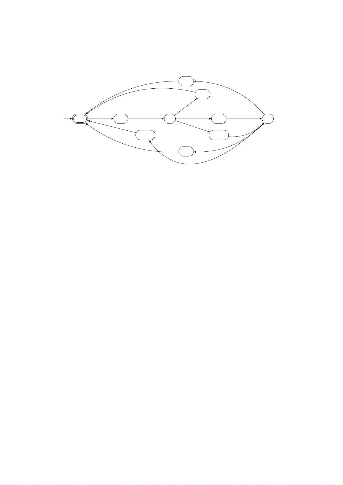
Practical Automated P artial V erification of Multi-P aradigm Real-Time Mo dels Carlo A. F uria, Matteo Pradella, and Matteo Rossi April 2008 Abstract This a rticle in tro duces a fully automated ver ification technique that p ermi ts to analyze rea l-time systems described using a c ontinuous notion of time and a mixtu re of operational (i.e., automata-based) and descriptive (i.e., logic-based) formalisms. The technique relies on th e reduction, u nder reasonable assumptions, of t h e conti nuous-time verification problem to its discrete-time counterpart. This reconciles in a viable and effective w ay t h e dense/discrete a nd op era tional/descriptive dic hotomies that are often en co untered in practice when it comes to sp eci fying and analyzing complex critical systems. The article inv estigates the applicability of the technique t hrough a significan t example centered on a comm u n ica tion protocol. More precisely , concurrent runs of th e proto co l are formalized by p ar allel instances of a Timed Au toma ton, while th e synchronization rules b et ween these instances are sp ecified th rough Metric T emporal Logic form ulas, t hus creating a multi-paradigm model. V erification tests run on this mo del using a b ounded v alidity chec ker implementi n g th e tec hn iq ue sho w consistent results and interesting p erformances. 1 Con ten ts 1 In tro duction 3 1.1 Overview . . . . . . . . . . . . . . . . . . . . . . . . . . . . . . . 4 1.2 Related W ork . . . . . . . . . . . . . . . . . . . . . . . . . . . . . 5 2 Preliminaries and Definitions 6 2.1 Behaviors . . . . . . . . . . . . . . . . . . . . . . . . . . . . . . . 6 2.2 Metric T empora l Logic . . . . . . . . . . . . . . . . . . . . . . . . 7 2.2.1 MTL + /MTL ∗ syntax and s eman tics. . . . . . . . . . . . . 8 2.2.2 Derived T empo ral Op erators . . . . . . . . . . . . . . . . 9 2.3 Op erational Mo del: Timed Automata . . . . . . . . . . . . . . . 9 2.4 Discrete-Time Approximations of Co n tin uous- Time Spec ific a tions . . . . . . . . . . . . . . . . . . . . . . . . . . . . . 11 2.4.1 Under- a nd Over-approximations of F ormulas . . . . . . . 12 2.4.2 System V e rification through Approximation . . . . . . . . 12 2.4.3 Discussion . . . . . . . . . . . . . . . . . . . . . . . . . . . 12 3 F ormali zi ng Timed Automata in MTL 13 3.1 Abo ut the Co rrectness and Co mpleteness of the Axiomatization . 15 4 Discrete-Time Approximations of Timed Automata 16 4.1 Under-approximation . . . . . . . . . . . . . . . . . . . . . . . . . 16 4.1.1 A New Axio matization . . . . . . . . . . . . . . . . . . . . 17 4.1.2 Clo c k C o nstrain ts . . . . . . . . . . . . . . . . . . . . . . 19 4.1.3 F o rm ulas (1 – 2 ) . . . . . . . . . . . . . . . . . . . . . . . . 19 4.1.4 F o rm ulas (3 – 4 ) . . . . . . . . . . . . . . . . . . . . . . . . 19 4.1.5 F o rm ulas (5 – 6 ) . . . . . . . . . . . . . . . . . . . . . . . . 19 4.2 Over-approximation . . . . . . . . . . . . . . . . . . . . . . . . . 20 4.2.1 Preliminarie s . . . . . . . . . . . . . . . . . . . . . . . . . 20 4.2.2 Clo c k C o nstrain ts . . . . . . . . . . . . . . . . . . . . . . 21 4.2.3 A ttempting F o rm ula (1) . . . . . . . . . . . . . . . . . . . 21 4.2.4 A New Axio matization . . . . . . . . . . . . . . . . . . . . 22 4.2.5 F o rm ulas (1 – 2 ) . . . . . . . . . . . . . . . . . . . . . . . . 23 4.2.6 F o rm ula (4) . . . . . . . . . . . . . . . . . . . . . . . . . . 23 4.2.7 Some Simplifications . . . . . . . . . . . . . . . . . . . . . 23 4.2.8 F o rm ulas (3),(5 – 6 ) . . . . . . . . . . . . . . . . . . . . . . 24 4.3 Summary . . . . . . . . . . . . . . . . . . . . . . . . . . . . . . . 24 5 Implementation and Example 25 5.1 T A Z ot . . . . . . . . . . . . . . . . . . . . . . . . . . . . . . . . . 25 5.2 A Communication Pr otocol Example . . . . . . . . . . . . . . . . 26 5.2.1 Description of the Proto col . . . . . . . . . . . . . . . . . 26 5.2.2 Prop erties of the System . . . . . . . . . . . . . . . . . . . 26 5.3 Exp erimen tal E v aluation . . . . . . . . . . . . . . . . . . . . . . . 28 6 Conclusion 30 2 1 In tro duction There is a tens io n be tw een the standp o in ts of mo deling and of verification when it comes to choosing a formal notation. The ideal mo deling langua g e would be very e xpressiv e, th us capturing so phisticated features of s ystems in a natur a l and straig h tforward manner; in particular, for concurr en t a nd real- time systems, a dense time mo del is the in tuitive choice to mode l true a sync hrony seamlessly . On the other hand, expressiveness is often tr aded off a g ainst co mplexit y (and decidability), hence the desire for a feasible and fully a uto mated verification pr o - cess pulls in the opp osite direction o f more pr imit ive, and less expressive, mo dels of time and systems. Discr ete time, for instance, is usually more amenable to automated verification, and q uit e mature techniques and to ols can b e deploy ed to verify s y stems mo deled under this ass um ption. Another, orthogo na l, concern of the real-time modeler is the choice b et ween op erational and descriptive mo deling language s . T ypical e x amples of op era- tional notations a r e Timed Automata (T A) and Timed Petri Nets, while tem- po ral lo gics ar e p opular instances of descriptive notations. Op erational and de- scriptive notations hav e complementary streng t hs and weaknesses. F o r instance, tempo ral log ics are very effective for describing par tia l mo dels or requirements ab out the past (thro ug h the natur a l use of past op erators); automata-based notations, o n the other hand, mo del systems throug h the notions o f sta te and transition, and a r e typically ea s y to sim ulate and visua lize. Hence, from a mo d- eling viewp oin t, the p o ssibilit y of integrating multiple mo deling pa radigms in formalizing a system would b e highly desirable. This pap er intro duces a verification tech nique tha t, under suitable assump- tions, reconciles the dense/discr ete a nd op erational/desc riptiv e dichotomies in an effective w ay . More pr e cisely: (1) it p ermits to analyze contin uous-time mo dels using fully a ut o ma ted, discrete-time verification techniques; and (2) it allows users to mix op erational (T A) and descriptive (metric temp oral log ic, MTL) comp onen ts in the system s p ecification. The technique is partia l in tw o resp ects: it ca n fail to provide conclusive a ns w ers, and only dense-time b eha v- iors with b ounded v aria bilit y are verified. It inv olves an automated translation of the o perationa l part into temp oral lo gic nota tio n, bas ed on a n MTL axiom- atization discussed in this pap er. The resulting MTL mo del, describing b oth the sy s tem and the pr operties to b e verified, is then dis cretized according to the techniques introduced in [16]. The discrete-time appr o ximation can b e an- alyzed through conv entional too ls; we pr ovide an implementation based o n the Z ot bo unded satisfiability chec ker [32]. W e exp erimen ted with a significant exa mple based on the descr iption of a communication pr otocol b y means o f a timed automaton. Co ncurren t r uns o f the proto col are for malized by pa rallel insta nces of the same a ut o maton; a ddi- tionally , the simple synchronization rules b et ween these insta nc e s is naturally formalized by means o f additional MTL formulas, hence building a mixed model. V er ification tests run on these models show ed consistent res ults, and acceptable per formances. An interesting auxiliar y con tribution of the discretizable ax iomatization of T A in MTL is a set of “ rules o f thum b” abo ut how to descr ibe systems based on the notion of state and transition with a logic forma lism, in a wa y which is als o amenable to discretization (according to the notion of [16]). Section 4 discusses this issue with g reat detail. 3 Finally , let us stress tha t our approa c h aims at providing a pr actic al approach to the verification of o perationa l (and mixed) mo dels. Hence, we sacrifice c o m- pleteness in or der to have a light weight and flexible technique. Also note that, although in this pap er T A are the o perationa l formalism of choice, the sa me approach could be applied to other op erational formalisms , suc h as Timed Petri Nets. Structure of the pap er. The pap er is org anized as follows. Section 1 .1 provides a sketc h of the whole technique with as little technical details a s p os- sible. Sec tion 1.2 briefly summarizes some r esearch rela t ed to the co n tent of this pap er. Section 2 introduces the tech nica l definitions that are needed in the remainder, na mely the syntax a nd semant ics of MTL and T A, a nd the dis- cretization techniques from [17, 16] that will b e used. Section 3 shows how to formalize the behavior of T A as a set of dense-time MTL for mulas. Then, Section 4 re-exa mines the axioms and suitably mo difies them in a w ay which is most amenable to the application of the discre tiza tion technique; the o ver- all res ult is a set of discr ete-time MTL formulas whose sa tisfiabilit y is linked to the satisfiability o f the orig inal dense - time fo r m ulas accor ding to the rules of the discr etization technique. Section 5 descr ib es the example of a simple communication proto col and r eports on the exp eriments conducted on it with the SA T-based implemen tatio n o f the technique. Finally , Section 6 draws s ome conclusions. 1.1 Ov erview The goal of our technique is to provide a means to carry out practica l verification techn ique o f r e al-time systems describ ed using a dense notion of time a nd a mix- ture of oper ational and descriptive notations. In particular, we assume a mo del of r e a l time ba sed on the notio n of b ehavi or , which is basically a contin uous-time signal, and we co ns ider a v ariant o f T A as op erational formalism and MTL a s descriptive formalism. The most common appr oac hes to similar verification pro blems in volve trans- lating the logic into automa ta [2]. In this paper we ta k e the mir ror a pproac h of descr ibing T A throug h MTL formulas. This choice is mainly justified by the fact that logic formulas are natura lly c ompositional, hence our ultimate goa l of formally combining mixed mo dels is fac ilita ted by this choice. It is well-known that MTL is undecidable ov er dens e time [4]; this hurdle is howev er pra ctically mitigated by employing the discr etization technique for MTL in tro duced — and demonstrated to b e practically appe aling — in [16]. Note that the undecidabil- it y of dense-time MTL en tails that the reduction technique m ust be incomplete, i.e., there are cases in which w e a re unable to hav e a conclusive outcome to the verification problem. How ever, as demo nstrated in [16], and further shown here, the impact of this sho rtcoming can b e rendered small in ma n y pra ctical cases. W e start by providing a dens e - time MTL axiomatization of T A. Notice that, due to a w ell- k no wn expres s iv eness ga p betw een temp oral lo gics and automata [23] it is impos s ible to describ e the la nguage a ccepted by a generic T A a s a n MTL formula. What we pr o vide is instead a for mal description of ac c epting runs o f a T A as an MTL for mula; in other words, we mode l the overall b eha vio r of T A with a set of MTL axio ms. The re s ultin g MTL a xioms are disc retized according to the rules provided in [16]. W e show that this yields po or r e sults 4 if done na ¨ ıvely; hence, we carefully revise the axiomatization a nd put it in a wa y which is muc h mo re amenable to discretiza tion. The result is a set of discretized MTL axioms describing T A runs. These ax ioms ca n b e combined with additional piece s of sp ecification, written in MTL, and with the pro p erties to be verified. The resulting complete mo del can then be a nalyzed by means of a utomated discrete-time to ols; the res ults of the discrete-time a na lysis are then used, as defined in [16], to finally infer results ab out the v er ific a tion of the original dense-time mo del. The exp erimental results are encour aging, b oth in terms o f perfo rmances and in terms of “c ompleteness cov erage” of the metho d. In this pap er we justify the soundness of the technique, which require s several analyses of the axioma tization and o f the discr etizations that are pr oduced. It is imp ortant to understand, how ever, that the r esulting technique (and to o l) is completely auto mated, and the user has just to pr o vide the dense-time mo del of the sy stem (i.e., T A and MTL form ulas ) and the putative pro perties to be verified. 1.2 Related W ork T o the b est of our knowledge, o ur approach is rather unique in try ing to com- bine o perational a nd descriptive formalis ms ov er dense time, then trading-o ff verification completeness against b etter perfor mance and practica l verification results. On the other hand, each of the “ingredients” of our method has b een studied in isolation in the literatur e . In this section we briefly recall a few of the most imp ortant results in this r espect. Dense-time verification of op erational mo dels is a very active field, a nd it has pro duced a few high-p erformance to ols a nd metho ds. Let us men tion, for instance, Uppaal [27], Kronos [3 5 ], HyT ech [21], and PHA V er [14] for the ver- ification o f timed (and h ybr id) automata . Notice that, although to ols s uc h as Uppaal allow the usage of a descriptive notation to express the prop erties to b e verified, the tempo ral logic subset is very simple and of very limited expressive power. In con tra s t, we allow basically full MTL to b e freely used in bo th the description of the mo del a nd in the for ma lization o f the prop erties to b e v er ifie d, at the pric e of sa crificing completeness of verification. Metric temp oral logic (MTL) verification is also a well-understo od resear ch topic. MTL is how ever known to b e undecidable ov er dense time doma ins [4]. A well-kno wn solution to this limitation restr icts the sy ntax of MTL formulas to disallow the expre s sion of exact (i.e., punctual) time distances [2]. The r esulting logic, called MITL, is fully de c ida ble over dense time. Ho wev er, the a ssociated decision pro cedures a re rather difficult to implemen t in practice and, even if re- cently significant progress ha s b een made in simplifying them [28], a serviceable implemen tatio n is s till lacking. Another stance at working a round the undecidability of dense-time MTL builds up on the fact that the s a me logic is decidable over discrete time. Hence, a few appro a c hes int r o duce s ome notion of discretization, that is par tial reduc- tion of the verification problem from de ns e to discrete time. The pres en t pap er go es in this direction by extending previous work on MTL [16] to the case of T A. A different discretization tec hnique, ba sed on the notion o f robust satis- fiability of MTL sp ecifications, has b een introduced in [13]. Other work also deals with notions of ro bustness in o rder to guara n tee that dense-time T A are implemen table with non-ideal architectures [11]. Another well-known no tio n o f 5 discretization is the one bas ed on the conce pt of digitization [22]; s ev eral author s hav e applied this quite general notion to the prac tica l verification of desc riptiv e [30, 2 4, 9 , 34] or op erational [20, 26, 7 , 6 , 29, 8, 5, 3 1 , 10] formalis ms. See also the related work section of [16] for more references a bout discr etization techn iques . 2 Preliminaries and Definitions 2.1 Beha viors Real-time sys tem mo dels describ e the temp oral b eha vior o f s ome basic items and propo sitions, which repr e s en t the observ able “fac ts ” of the s ystem. Mor e precisely , an item it is characterized b y a finite domain D it (and w e wr ite it : D it ) such that a t a n y insta nt of time it ta k es o ne of the v alues in D it . On the o ther hand, a prop osition p is simply a fact which can b e true or fals e at any instan t of time. A b ehavior is a formal mo del o f a tr ac e (or run ) o f some r eal-time system. Given a time domain T , a finite set P of atomic prop ositions, and a finite set o f items I , a b eha vior b is a mapping b : T → D it 1 × D it 2 × · · · × D it |I| × 2 P which asso ciates with every time insta n t t ∈ T the tuple b ( t ) = h v 1 , v 2 , . . . , v |I | , P i of item v alues and prop ositions that are tr ue at t . B T denotes the set of all behaviors ov er T , for an implicit fixed set of items and prop ositions. b ( t ) | it and b ( t ) | P denote the pro j ectio n o f the tuple b ( t ) over the comp onen t corres p onding to item it and the set of pro positions in 2 P resp ectiv ely . Also, t ∈ T is a tr ansition p oint for b ehavior b if t is a disc o n tinu ity p oin t of the mapping b . Whether T is a discrete, de ns e, o r con tinuous set, we call a b eha vio r ov er T discrete-, dense-, or cont inuous-time resp ectively . In this pap er, we consider the natural num b ers N as discrete- tim e domain and the nonnegative real num b ers R ≥ 0 as contin uous- t ime (and dense-) time domain. Non-Zeno and non-Berkeley . Over dense-time domains, it is customary to consider only physically mea ningful b eha viors , namely those resp ecting the so- called non-Z eno pro p erty . A behavior b is non-Zeno if the sequence of tr ansition po in ts of b has no accumulation p oin ts. F or a non- Zeno b eha vior b , it is well- defined the notions of v alues to the left and to the right of an y transition p oin t t > 0 , whic h we denote as b − ( t ) a nd b + ( t ), resp ectiv ely . In this pap er, we are in ter e s ted in b ehaviors with a stronger requirement, called non-Berkeleyness . Infor mally , a be havior b is non- B erk eley for some po s- itive constant δ ∈ R > 0 if, for all t ∈ T , there exists a clos e d interv al [ u , u + δ ] of size δ s uch that t ∈ [ u, u + δ ] and b is cons t a n t throug hout [ u, u + δ ]. Notice that a non-Berkeley b ehavior (for any δ ) is non-Zeno a fortiori . The set of all non-B erk eley dense-time behaviors for δ > 0 is denoted by B δ χ ⊂ B R ≥ 0 . In the following we alwa ys assume b ehaviors to b e non-Be rk eley , unless ex plicitly stated otherwise. Syn tax and seman ti cs. F ro m a purely s eman tic point of view, a (real-time) system mo del is simply a set of behaviors [3, 1 5] o ver some time domain T a nd sets of items a nd prop ositions. In practice, how ever, the mo deler sp ecifies a 6 system thr ough some suitable notation. In this pa per we consider Metric T e m- po ral Logic (MTL) [25, 4] as descriptive nota tio n, and T A [1, 2] a s op erational notation. Their sy ntax and semantics ar e defined in the following. Given an MTL formula or a T A µ , and a b eha vior b , we write b | = µ to denote that b des cribes a system evolution which satisfies all the constr ain ts impo sed by µ . If b | = µ for some b ∈ B T , µ is called T -sa tisfiable; if b | = µ for all b ∈ B T , µ is called T -v alid. Similarly , if b | = µ for some b ∈ B δ χ , µ is called χ δ -satisfiable; if b | = µ for all b ∈ B δ χ , µ is ca lled χ δ -v alid. 2.2 Metric T emp oral Logic Let P be a finite (no n- empt y) set o f a tomic prop ositions, I b e a finite set of items, and J be the set o f all (p ossibly unbounded) interv a ls of the time domain T with ratio nal endp oin ts. 1 Usually , one considers interv als with non- negative e ndp oints, but we p ermit nega tiv e endp oin ts to render the pre s en tation more unifor m and straig h tforward. Also , we abbrevia te interv als with pseudo - arithmetic expr essions, such as = d , < d , ≥ d , for [ d, d ], (0 , d ), and [ d, + ∞ ), resp ectiv ely . MTL syntax. The following grammar defines the syntax of MTL, wher e I ∈ J and β is a Bo olean combination o f atomic prop ositions or conditions ov er items, i.e., β ::= p | it = v | ¬ β | β 1 ∧ β 2 for p ∈ P , it ∈ I , v ∈ D it . 2 φ ::= β | φ 1 ∨ φ 2 | φ 1 ∧ φ 2 | U I ( β 1 , β 2 ) | S I ( β 1 , β 2 ) | R I ( β 1 , β 2 ) | T I ( β 1 , β 2 ) In order to ease the presentation of the discretizatio n techniques in Section 2.4, MTL formulas are intro duced in a flat nor mal form where nega tions a r e pushed down to (Bo olean combinations o f ) atomic prop ositions, and temp oral op erators are not nested. It sho uld b e clear, how ever, tha t any MTL form ula can b e put in to this form, p ossibly b y intro ducing auxilia ry prop ositional letters [12, 19]. The basic temp oral op erators of MTL ar e the b ounde d u ntil U I (and its past co un terpart b ounde d sinc e S I ), as well as its dual b ounde d r ele ase R I (and its past co un terpart b ounde d trigger T I ). The subscr ipts I denote the interv al of time ov er which every op erator predicates . In the following we assume a num b er of standar d abbrev ia tions, such a s ⊥ , ⊤ , ⇒ , ⇔ , and, when I = (0 , ∞ ), we drop the subscript int er v al of ope r ators. The precedence order of logic connectiv es is, from the o ne of highest binding power: ¬ , ∧ , ∨ , ⇒ , ⇔ . MTL s e man tics. MTL semantics is defined over b eha viors , para met r ically with resp ect to the choice of the time doma in T . 1 That i s any I ∋ I = h l, u i for some l ≤ u where l ∈ T ∩ Q and u ∈ ( T ∩ Q ) ∪ {±∞} , h is one of ( and [ , and similarly for i . 2 Note that ¬ ( it = v ) can be abbreviated as it 6 = v . 7 b ( t ) | = T p iff p ∈ b ( t ) | P b ( t ) | = T ¬ p iff p 6∈ b ( t ) | P b ( t ) | = T it = v iff v = b ( t ) | it b ( t ) | = T it 6 = v iff v 6 = b ( t ) | it b ( t ) | = T U I ( β 1 , β 2 ) iff there ex ists d ∈ I such that: b ( t + d ) | = T β 2 and, for all u ∈ [0 , d ] it is b ( t + u ) | = T β 1 b ( t ) | = T S I ( β 1 , β 2 ) iff there ex ists d ∈ I such that: b ( t − d ) | = T β 2 and, for all u ∈ [0 , d ] it is b ( t − u ) | = T β 1 b ( t ) | = T R I ( β 1 , β 2 ) iff for a ll d ∈ I it is : b ( t + d ) | = T β 2 or there ex ists a u ∈ [0 , d ) such that b ( t + u ) | = T β 1 b ( t ) | = T T I ( β 1 , β 2 ) iff for a ll d ∈ I it is : b ( t − d ) | = T β 2 or there ex ists a u ∈ [0 , d ) such that b ( t − u ) | = T β 1 b ( t ) | = T φ 1 ∧ φ 2 iff b ( t ) | = T φ 1 and b ( t ) | = T φ 2 b ( t ) | = T φ 1 ∨ φ 2 iff b ( t ) | = T φ 1 or b ( t ) | = T φ 2 b | = T φ iff for a ll t ∈ T : b ( t ) | = T φ W e remar k that a global sa tisfiabilit y sema n tics is assumed, i.e ., the satis- fiability of formulas is implicitly ev aluated ov er al l time instants in the time domain. This pe r mits the dire c t and natural expression o f most common real- time sp ecifications (e.g., time-b ounded resp onse) without resorting to nesting of tempo ral op erators. Also notice that our MTL v ariant uses op erators that are non-strict in their fir st argument, i.e., the future and past include the present instant, and the until and sinc e op erators are matching , i.e., they require their t wo ar gumen ts to hold to gether at some ins tan t in I . Other work [18] analyzes the impact of these v aria n ts on expres siv eness. Gran ularit y . F or an MTL for m ula φ , let J φ be the s e t o f all no n-n ull, finite int er v al bounds app earing in φ . Then, D φ is the se t o f p ositiv e v alues δ such that any int er v al bo und in J φ is a n integer if divided by δ . 2.2.1 MTL + /MTL ∗ syn tax and sem an ti c s . In orde r to e x press the dis cretization relations in Section 2 .4 , it is necessary to in tro duce some v ar iations of the four basic temp oral o perator s until , sinc e , r ele ase , and trigger , denoted as U ↑ I , S ↑ I , R ↓ I , and T ↓ I , resp ectiv ely . Notice that they are not par t of the language in which dens e-time sp ecifications and prop erties are to b e expres sed, and they ar e needed only to illustrate the discretiza tion techn iques . W e ca ll “MTL + ” the exten si on o f MTL with these op erators , and “MTL ∗ ” the v ariant where we r eplac e the ope r ators U I , S I , R I , T I with U ↑ I , S ↑ I , R ↓ I , and T ↓ I , res pectively . Let us define the sema n tics of the new v ariants of until and r ele ase . b ( t ) | = T U ↑ I ( β 1 , β 2 ) iff there exists d ∈ I such that: b ( t + d ) | = T β 2 and, for all u ∈ [0 , d ) it is b ( t + u ) | = T β 1 b ( t ) | = T S ↑ I ( φ 1 , φ 2 ) iff there exists d ∈ I such that: b ( t − d ) | = T φ 2 and, for all u ∈ [0 , d ) it is b ( t − u ) | = T φ 1 b ( t ) | = T R ↓ I ( φ 1 , φ 2 ) iff for all d ∈ I it is: b ( t + d ) | = T φ 2 or there ex ists a u ∈ [0 , d ] such that b ( t + u ) | = T φ 1 b ( t ) | = T T ↓ I ( φ 1 , φ 2 ) iff for all d ∈ I it is: b ( t − d ) | = T φ 2 or there ex ists a u ∈ [0 , d ] such that b ( t − u ) | = T φ 1 8 2.2.2 Derived T emp oral O perators It is useful to introduce a num b er of derived temp oral op erators, to be used as shorthands in wr iting sp ecification for m ulas. W e consider those listed in T able 1 ( δ ∈ R > 0 is a par ameter tha t will b e used in the discr etization technique describ ed shortly). Opera tor ≡ Definition ♦ I ( β ) ≡ U I ( ⊤ , β ) ← − ♦ I ( β ) ≡ S I ( ⊤ , β )  I ( β ) ≡ R I ( ⊥ , β ) ← −  I ( β ) ≡ T I ( ⊥ , β ) f  ( β ) ≡ U (0 , + ∞ ) ( β , ⊤ ) ∨ ( ¬ β ∧ R (0 , + ∞ ) ( β , ⊥ )) f ← −  ( β ) ≡ S (0 , + ∞ ) ( β , ⊤ ) ∨ ( ¬ β ∧ T (0 , + ∞ ) ( β , ⊥ ))  ( β ) ≡ β ∧ f  ( β ) ← −  ( β ) ≡ β ∧ f ← −  ( β ) △ ( β 1 , β 2 ) ≡    f ← −  ( β 1 ) ∧  β 2 ∨ f  ( β 2 )  if T = R ≥ 0 ← − ♦ =1 ( β 1 ) ∧ ♦ [0 , 1] ( β 2 ) if T = N N ( β 1 , β 2 ) ≡ ( β 1 ∧ ♦ = δ ( β 2 ) if T = R ≥ 0 β 1 ∧ ♦ =1 ( β 2 ) if T = N T able 1 : MTL derived temp oral o perator s Let us describ e infor mally the mea ning of such derived o perator s, fo cusing on future ones (the meaning o f the corres p onding pas t op erators is easily deriv able). ♦ I ( β ) means tha t β happ ens within time interv al I in the future.  I ( β ) means that β holds thro ug hout the whole interv al I in the future. f  ( β ) denotes that β holds thro ughout some no n-empt y interv al in the strict future; in other words, if t is the cur ren t instant, there exists s o me t ′ > t such that β holds ov er ( t, t ′ ). Similarly ,  ( β ) denotes that β holds throughout some non-e mpty interv al which includes the current instant, i.e., over so me [ t, t ′ ). Then, △ ( β 1 , β 2 ) des c ribes a switch from conditio n β 1 to condition β 2 , without sp ecifying which v a lue holds at the current instan t. On the o ther hand, N ( β 1 , β 2 ) describ es a switch fro m condition β 1 to condition β 2 such that β 1 holds a t the current instant. In addition, for an item it we int r oduce the shor thand △ ( it , v − , v + ) for △ ( it = v − , it = v + ). A similar abbrevia tion is assumed for N ( it , v − , v + ). Finally , let us abbre viate b y Alw ( φ ) the nesting MTL for m ula φ ∧  (0 , + ∞ ) ( φ ) ∧ ← −  (0 , + ∞ ) ( φ ); b | = T Alw( φ ) iff b | = T φ , for any b e ha vior b , s o Alw( φ ) can b e ex- pressed without nes t ing if φ is fla t , thro ugh the global satisfiability semantics int ro duced b eforehand. 2.3 Op erational Mo del: Timed Automata W e introduce a v ariant of T A which differs from the cla s sical definitions (e.g., [1]) in that it r ecognizes behaviors, rather than timed words [2, 28]. Cor r espondingly , input s ym bo ls are asso ciated with lo cations rather than with trans itions. Also, 9 we introduce the following simplifications that a r e known to b e without loss of generality: we do not define lo cation clo c k inv ariants (also called staying conditions) and use tr a nsition guards only , and we forbid self-lo op transitions . On the other hand, we introduce one additional v ar ian t which does im- pact e xpressiv enes s , namely clo c k constr ain ts do not distinguish betw een dif- ferent transition edges, that is b et ween trans itio ns o ccurring right- and left- contin uously . This res triction is motiv ated by our ultimate g oal of discr etizing T A: a s it will b e expla ined later, such distinctions would inevita bly b e lost in the discretization pro cess, hence we give them up already . Finally , for the sa k e of simplicity , let us not consider acceptance co ndit io ns, that is let us ass ume that all states a re acce pting . No te, how ever, that introduc- ing a cceptance conditions (e.g ., B ¨ uchi, Muller, etc.) in the formaliza tion w ould be r outine. Timed automata syn tax. F or a set C of clo c k v aria bles, the set Φ( C ) of clo ck c onstr aints ξ is defined inductively by ξ ::= c < k | c ≥ k | ξ 1 ∧ ξ 2 | ξ 1 ∨ ξ 2 where c is a clo c k in C and k is a consta n t in Q ≥ 0 . A time d automaton A is a tuple h Σ , S, S 0 , α, C , E i , wher e: • Σ is a finite (input) alphab et, • S is a finite set of lo cations, • S 0 ⊆ S is a finite s et of initia l lo cations, • α : S → 2 Σ is a loca tion lab eling function that assigns to each lo cation s ∈ S a set α ( s ) of pr opositions, • C is a finite set of clo cks, and • E ⊆ S × S × 2 C × Φ( C ) is a set of transitio ns . An edge h s, s ′ , Λ , ξ i r epresen ts a transition from state s to state s ′ 6 = s ; the s et Λ ⊆ C identifies the clo cks to b e r eset with this transition, and ξ is a clo c k constraint ov er C . Timed automata semant i c s. In defining the seman tics of T A over b ehav- iors we dev iate from the standard pre sen tation (e.g., [2, 2 8 ]) in that we do not represent T A as acceptor s o f behaviors o ver the input alpha bet Σ, but rather as acceptors of b eha vio r s representing what are usually called runs o f the automa- ton. In o th er words, we introduce automata as accepto rs of b eha viors ov er the items st and in r epresen ting resp ectiv ely the cur ren t lo cation and the current input symbol, as well a s pr opositions rs c | c ∈ C representing the c lock res et status. This departure fr om more traditiona l pr esen tations is justified by the fact that we intend to provide an MTL axio matic description of T A runs — r ather than accepted langua ges, which w ould b e impossible for a well-known expres siv eness gap [23] — hence we define the semantics of automata ov er this “extended” state fro m the b eginning. Let us firs t define the semantics only informally . Initially , all clo c ks are reset and the a utomaton sits in some state s 0 ∈ S 0 . At any given time t , when the automaton is in so me state s , it can take nondeterministica lly a trans ition to 10 some other state s ′ such that h s, s ′ , Λ , ξ i is a v alid tr a nsition, provided the last time (befo r e t ) each clo ck has b een reset is co mp a t ible with the constr ain t ξ . If the transition is taken, all clo c ks in Λ a re reset, wher eas a ll the other clo c ks keep on running unc hang ed. Finally , as long as the automaton sits in any s tate s , the input ha s to satisfy the lo cation lab eling function α ( s ), namely the curr en t input co rrespo nds to exa ctly one o f the prop ositions in α ( s ). F o rmally , a timed automaton A = h Σ , S, S 0 , α, C , E i is interpreted over be - haviors ov er items s t : S, in : Σ and pro positions R = { rs c } c ∈ C . Intuitiv ely , at any instant of time t , st = s mea ns that the automaton is in state s , in = σ means that the automato n is reading symbol σ , and rs c keeps tra c k of res e ts of clo ck c (more precisely , we mo del such resets throug h switc hes, from fa ls e to true or vic e versa , of rs c ). Let b b e such a behavior, and let t be one o f its tr ansition p oin ts. Satisfaction of clo c k cons tr ain ts a t t is defined as follows: b ( t ) | = c < k iff either b − ( t ) | = rs c and there exists a t − k < t ′ < t such that b ( t ′ ) 6| = rs c ; or b − ( t ) 6| = rs c and there exists a t − k < t ′ < t such that b ( t ′ ) | = rs c b ( t ) | = c ≥ k iff either b − ( t ) | = rs c and for all t − k < t ′ < t : b ′ ( t ) | = rs c ; or b − ( t ) 6| = rs c and for all t − k < t ′ < t : b ( t ′ ) 6| = rs c Notice tha t this corresp onds to lo oking for the previous time the pr o position rs c switched (from false to true or from true to false) and counting time since then. This requires a little hack in the definition of the semantics: namely , a fir st start reset of all clo c ks is issued b efore the “r eal” run b egins; this is repr esen ted by time instant t start in the formal semantics b elow. Then, a b eha vio r b ov er st : S, in : Σ , R (with b : R ≥ 0 → S × Σ × 2 R ) is a run of the automaton A , and we write b | = R ≥ 0 A , iff: • b (0) = h s 0 , σ, S c ∈ C { rs c }i a nd σ ∈ α ( s 0 ) for s o me s 0 ∈ S 0 ; • there exists a trans ition instant t start > 0 such that: b ( t ) | st = s 0 and b ( t ) | R = R for all 0 ≤ t ≤ t start , b − ( t start ) = h s 0 , σ − , ρ − i and b + ( t start ) = h s + , σ + , ρ + i with ρ − = R and ρ + = ∅ ; • for a ll t ∈ R ≥ 0 : b ( t ) | in ∈ α ( b ( t ) | st ); • for a ll transition instants t > t start of b | st or b | R such that b − ( t ) = h s − , σ − , ρ − i and b + ( t ) = h s + , σ + , ρ + i , it is: h s − , s + , Λ , ξ i ∈ E , σ − ∈ α ( s − ), σ + ∈ α ( s + ), ρ = S c ∈ Λ { rs c } , ρ + = ρ − △ ρ = ( ρ − \ ρ ) ∪ ( ρ \ ρ − ), and b ( t ) | = ξ . 2.4 Discrete-Time A pp roxima t ions of Con tinuous -Time Sp ecifications In [16] w e pr e sen ted a technique to r educe the v alidity pro blem for MTL specifi- cations over dense time to the same problem ov er discrete time. In this section we concisely summarize the fundamen tal results fro m [1 6 ] that ar e needed in the rema inder of the pa p er, and we pro vide some int uition ab out how they can be a pplied to our discretization problem. 11 2.4.1 Under- and Over-appro ximations of F orm ulas W e in tro duce tw o appr o ximations of MTL formulas, called under- and over-ap- proximation. Under-appro ximation. The approximation function Ω δ ( · ) maps dense- tim e MTL formulas to discrete-time MTL ∗ formulas such tha t the non-v alidity of the latter implies the no n-v alidity o f the former, ov er b e haviors in B δ χ . More precisely , for MTL formu la s such that the c hos en sampling p eriod δ is in D φ , Ω δ ( · ) is defined as fo llo ws. Ω δ ( β ) ≡ β Ω δ ( φ 1 ∧ φ 2 ) ≡ Ω δ ( φ 1 ) ∧ Ω δ ( φ 2 ) Ω δ ( φ 1 ∨ φ 2 ) ≡ Ω δ ( φ 1 ) ∨ Ω δ ( φ 2 ) Ω δ  U h l,u i ( φ 1 , φ 2 )  ≡ U ↑ [ l/δ,u/δ ] (Ω δ ( φ 1 ) , Ω δ ( φ 2 )) Ω δ  S h l,u i ( φ 1 , φ 2 )  ≡ S ↑ [ l/δ,u/δ ] (Ω δ ( φ 1 ) , Ω δ ( φ 2 )) Ω δ  R h l,u i ( φ 1 , φ 2 )  ≡ R ↓ h l/δ,u/δ i (Ω δ ( φ 1 ) , Ω δ ( φ 2 )) Ω δ  T h l,u i ( φ 1 , φ 2 )  ≡ T ↓ h l/δ,u/δ i (Ω δ ( φ 1 ) , Ω δ ( φ 2 )) Ov er-appro xim a tio n. The approximation function O δ ( · ) maps dense- tim e MTL for m ulas to discr ete-time MTL for m ulas such tha t the v alidity of the latter implies the v alidity of the former , over behaviors in B δ χ . Mo re pre cisely , for MTL formulas such that the c ho s en sampling per iod δ is in D φ , O δ ( · ) is defined as follows. O δ ( β ) ≡ β O δ ( φ 1 ∨ φ 2 ) ≡ O δ ( φ 1 ) ∨ O δ ( φ 2 ) O δ ( φ 1 ∧ φ 2 ) ≡ O δ ( φ 1 ) ∧ O δ ( φ 2 ) O δ  U h l,u i ( φ 1 , φ 2 )  ≡ U [ l/δ +1 , u/δ − 1] (O δ ( φ 1 ) , O δ ( φ 2 )) O δ  S h l,u i ( φ 1 , φ 2 )  ≡ S [ l/δ +1 , u/δ − 1] (O δ ( φ 1 ) , O δ ( φ 2 )) O δ  R h l,u i ( φ 1 , φ 2 )  ≡ R [ l/δ − 1 ,u/δ +1] (O δ ( φ 1 ) , O δ ( φ 2 )) O δ  T h l,u i ( φ 1 , φ 2 )  ≡ T [ l/δ − 1 ,u/δ +1] (O δ ( φ 1 ) , O δ ( φ 2 )) 2.4.2 System V erification through Approximation W e hav e the following fundamental v er ific a tion res ult from [16], which provides a justificatio n for the T A verification tech nique dis cussed in this pap er. Prop osition 1 (Appro ximations [16 ]) . F or any MTL formulas φ 1 , φ 2 , and for any δ ∈ D φ 1 ,φ 2 : (1) if Alw (Ω δ ( φ 1 )) ⇒ Alw( O δ ( φ 2 )) is N -valid, then Alw( φ 1 ) ⇒ Alw ( φ 2 ) is χ δ -valid; and (2) if Alw (O δ ( φ 1 )) ⇒ Alw( Ω δ ( φ 2 )) is not N -valid, then Alw ( φ 1 ) ⇒ Alw( φ 2 ) is not χ δ -valid. 2.4.3 Dis cuss ion Prop osition 1 sug gests a verification tec hnique which builds tw o for m ulas through a suitable compo sition of ov er - and under-approximations of the sys tem descrip- tion and the putativ e pr operties, and it infers the v alidit y o f the prop erties fro m 12 the r esults of a disc rete-time v alidit y ch ecking. The technique is incomplete as, in particula r, when appr o ximation (1) is not v alid and a ppro ximation (2) is v alid w e cannot infer an ything ab out the v alidit y of the prop ert y in the or iginal system over dense time. Let us now provide some evidence ab out why different, but equiv alent, dense- time formulas can yield dramatica lly differe nt — in terms o f usefulness — ap- proximated discre te- tim e formulas. W e provide one in-the-s ma ll example for ov er-appr o ximations a nd o ne for under-approximations. More concrete exam- ples will appear in Section 4 when building appr o ximations of T A’s axiomatic description. Let us co nsider dense-time MTL formula θ 1 =  (0 ,δ ) ( p ) which, under the global satisfiability semantics, says that p is always tr ue. Its under-a ppro xi- mation is Ω δ ( θ 1 ) =  ∅ ( p ) which holds for any discrete-time b e ha vior! Thus, we hav e an under-approximation which is likely too coar se, as it basica lly adds no info r mation to the discrete-time r epresen tation. So , if w e build for m ula (1) from Prop osition 1 w ith Ω δ ( θ 1 ) in it, it is most likely that the anteceden t will be tr iv ially satisfiable (be cause Ω δ ( θ 1 ) in tro duces no co ns train t) a nd hence formula (1) will b e no n-v alid, y ie lding no informa tio n to the verification pro cess. If, howev er, we mo dify θ 1 int o the e quivalent θ ′ 1 = p ∧ θ 1 we get an under-ap- proximation which can be written as simply Ω δ ( θ ′ 1 ) = p , which corr ectly en tails that p is a lw ays true ov er discre te- tim e as well. This is lik ely a m uch be tter approximation, one which b etter preser v es the origina l “ meaning” of θ 1 . Let us now co nsider dense-time MTL formula θ 2 = ♦ [0 , 2 δ ] ( p ), whic h describ es a prop osition p which is false for no longer than 2 δ time units. If we compute its over-approximation, we get O δ ( θ 2 ) = ♦ =1 ( p ) which, under the global satisfi- ability seman tics, entails that p is always true. Although the actual assessment depe nds o n the ro le θ pla ys in the ov er all sp ecification, it is likely that this ov er-appr o ximation is to o coarse, as it bas ically adds “to o str ong” informatio n to the discrete-time repr esen tation. So , if we build formula (2) fro m P r oposition 1 with O δ ( θ 2 ) in it, it is very lik ely that the a n tecedent will be unsatisfia ble (beca use O δ ( θ 2 ) intro duces a v ery stro ng cons tr ain t) and hence formu la (2 ) will be v alid, yielding no information to the v er ific a tion pro cess. On the contrary , if we simply mo dify θ 2 int o the e quivalent θ ′ 2 = p ∨ θ 2 we get a n ov er - appro xi- mation which can be wr itten as O δ ( θ ′ 2 ) = ♦ [0 , 1] ( p ), i.e., p is fa lse no more tha n every tw o time steps. This lo oks like a muc h b etter appr o ximation, one which better preserves the orig inal “meaning” of θ 2 . 3 F ormalizing Timed Automata in MTL Let us cons ide r a timed automaton A = h Σ , S, S 0 , α, C , E i and let us for malize its runs ov er non-Berkeley b ehaviors for s ome δ > 0. In o ther words, we a r e going to provide a set of formulas φ 1 , . . . , φ 6 such that, for all non-Berkeley behaviors b , b | = A iff b | = φ j for a ll j = 1 , . . . , 6. T ranslating clo c k constrain ts. W e as sociate a n MTL formula Ξ( ξ ) to ev er y clo c k co nstrain t ξ such that b ( t ) | = ξ iff b ( t ) | = Ξ( ξ ) at all transition points t . 13 Ξ( ξ ) can b e defined inductiv ely a s: Ξ ( c < k ) ≡ f ← −  ( rs c ) ∧ ← − ♦ (0 ,k ) ( ¬ rs c ) ∨ f ← −  ( ¬ rs c ) ∧ ← − ♦ (0 ,k ) ( rs c ) Ξ ( c ≥ k ) ≡ f ← −  ( rs c ) ∧ ← −  (0 ,k ) ( rs c ) ∨ f ← −  ( ¬ rs c ) ∧ ← −  (0 ,k ) ( ¬ rs c ) ξ 1 ∧ ξ 2 ≡ Ξ 1 ∧ Ξ 2 ξ 1 ∨ ξ 2 ≡ Ξ 1 ∨ Ξ 2 Basically , Ξ transla tes the guard ξ by c omparing the curr en t time to the la st time a res e t for the clo c k c happ ened, where a r eset is signaled by a s witc hing of item rs c . Notice that this assumes the existence o f a “firs t res et” of all clo c ks, as specified in the formal seman tics of T A, and as will be p ostulated in F o rm ula (5) b elow. Also notice that, when co mpu ting the approximations of the clo c k- constraint formulas, w e will hav e to require tha t every co nstan t k used in the definition of the T A is an integral multiple o f δ . Necessary conditio ns for s ta te c hange. Let us state the necessa ry co ndi- tions that character iz e a state change. F or any pair o f states s i , s j ∈ S such that there ar e K transitions h s i , s j , Λ k , ξ k i ∈ E for all 1 ≤ k ≤ K , we intro duce the axiom: △ ( st , s i , s j ) ⇒ _ k Ξ( ξ k ) ∧ ^ c ∈ Λ k  △ ( ¬ rs c , rs c ) ∨ △ ( rs c , ¬ rs c )  (1) Complementarily , we int r o duce an ax io m to a s sert that for an y pair o f states s i 6 = s j ∈ S suc h that h s i , s j , Λ , ξ i 6∈ E for a n y σ , Λ , ξ , i.e., for any pair of states that are not co nnected by any edge: ¬△ ( st , s i , s j ) (2) Sufficien t conditions for state c hange. W e have multiple sufficien t con- ditions for state changes; basically , they account for reactions to reading input symbols and r esetting clo c ks. Let us consider input first: the staying co ndit io n in every state mu st b e satisfied always, so for all s ∈ S we add the axiom: st = s ⇒ in ∈ α ( s ) (3) Then, fo r each rese t o f a clock c ∈ C , le t us consider all edges of the form h s k i , s k j , Λ k , ξ k i ∈ E , such that c ∈ Λ k . Hence, we introduce the pair of a xioms: △ ( ¬ rs c , rs c ) ⇒ _ k △  st , s k i , s k j  △ ( rs c , ¬ rs c ) ⇒ _ k △  st , s k i , s k j  ∨ _ s 0 ∈ S 0 ← −  (0 , + ∞ ) ^ c ∈ C rs c ∧ st = s 0 ! (4) Note that the seco nd a xiom has an additiona l part that takes into account the instants b efore the fir s t r eset (which must o ccur somewhere as shown in (5), and which cor responds to the instants befor e t start in the forma l s eman tics), w her eas the first o ne is not applicable be f o r e such a firs t reset. 14 Initialization and liveness conditi o n. W e complete o ur axiomatiza tion by first des cribing the system initialization. W e r emark that the following axiom is only ev aluated at 0. Notice that, under the global sa t isfia bilit y semantics and with a mono- infinite time do main, a formula φ 0 that should b e only ev aluated at 0 can b e expressed a s ← −  ( ⊥ ) ⇒ φ 0 , as ← −  ( ⊥ ) holds only where there is no pa st, i.e., at 0. at 0 : ^ c ∈ C rs c ∧ ♦ [0 , 2 δ ] ^ c ∈ C ¬ rs c ! ∧ _ s 0 ∈ S 0  ( st = s 0 ) (5) Notice that we make the axioma tization slig h tly more “deterministic” than the formal semant ics, in that w e require that t start , when the first reset of the clo c ks o ccurs, is betw een 0 a nd 2 δ ; this, combined with the non-Berkeleyness requirement, says that it actually o ccurs b et ween δ and 2 δ . All in all, (5) pictures the fo llowing initialization: • rs c holds over [0 , δ ] for all c ∈ C ; • rs c switches to false at some t start ∈ ( δ, 2 δ ] for all c ∈ C (clea rly , this tran- sition p oin t is the same fo r a ll c ∈ C , still bec a use of the non-Ber keleyness assumption); • st = s 0 holds fo r so me s 0 ∈ S 0 ov er [0 , δ ]; • beca use of the non-Berkeleyness assumption, if st changes in ( δ, 2 δ ] it do es so together with the rese t s at t start ; • △ ( rs c , ¬ rs c ) holds at t start for all c ∈ C ; the c o nsequen t of (4) is tr ue bec ause o f the disjunct ← −  (0 , + ∞ )  V c ∈ C rs c ∧ st = s 0  which holds at t start . Finally , often we in tro duce a “liveness” co ndition which sta tes that we even- tually have to move out of every state, co rresponding to the fact that a ll states are accepting ` a la B¨ uchi. Thus, for every state s ∈ S , let S ′ s ⊂ S b e the set of states that are directly reachable from s through a sing le transition; then we consider the axiom: st = s ⇒ ♦   _ s ′ ∈ S ′ s st = s ′   (6) 3.1 Ab out t he Correctness and Completeness of the Ax- iomatization W e o mit a pro of o f the completeness and correctnes s of the a xiomatization; we refer the r eader to [19, App. D.6] wher e a pro of for a similar a xiomatization is sketc hed. Here, we just add a few rema rks that can help justify the cor rectness and a ppropriateness of the present axiomatizatio n. Prop osition 2 (MTL T A Axio matization) . L et A = h Σ , S, S 0 , α, C , E i b e a time d automaton, φ A 1 , . . . , φ A 6 b e formulas (1–6) for T A A, and let b ∈ B δ χ b e any non-Berkeley b ehavior over items st : S, in : Σ and pr op ositions in R . Then b | = A for some t start ∈ ( δ, 2 δ ) 3 if and only if b | = V 1 ≤ j ≤ 6 φ A j . 3 This additional condition i s introduced t o tak e in to account the particular f orm of the initialization axiom (5). 15 State c hanges can o ccur rig h t- or left-con tinuously . It sho uld b e clear that the above axiomatiza tion with the b e c omes opera tors do es not force any item to tra nsition either r igh t- or left-contin uously; in fact, the op erator a llo ws bo th p ossibilities. Over dense time, how ever, it would hav e b een p o ssible to force tr ansitions to o ccur either alwa ys r igh t- or alwa ys left-co ntin uous ly . F or instance, r igh t-contin uity can be a c hieved in one of the following wa ys: • add for mulas such as f  ( st = s i ) ⇒ s i ; • add for mulas such as ¬  ← −  ( st = s i ) ∧ f  ( st = s j )  . Corresp ondingly , the whole formaliza tion could hav e b een simplified a bit taking int o acco un t this new pro p erty . Unfortunately , how ever, it is not difficult to see that a ll solutio ns would yield very p oor dis c rete-time ov er-approximations, wher e by very po or we mean comprising only very trivial b ehaviors, and thus offering a very weak supp ort to verification. F or insta nce , the ov er- and under-approximations of  ( st = s i ) ⇒ s i would require st to s tay equal to s i forever once it takes suc h v alue. Intuitiv ely , this is due to the fact that a fine-grained informatio n suc h a s the edge of items at tr ansition po in ts is lost with a finite-precisio n sa mpling. There ma y be w or k- arounds for this, but it seems that they are overly co mplex. On the other hand, forgetting ab out characterizing transitio ns as rig h t- or left-contin uous allows us to get a m uch mo re straig h tforward axio matization while still ge tting our approximations to work reasona bly well. 4 Discrete-Time Appro ximations of Timed Au- tomata Let us s ho w how to compute the under- and ov er-approximation of formulas (1 – 6) in a s uita ble w ay . 4.1 Under-appro ximation The particular form of formulas (1 – 2),(4) is unsuitable to pro duce under- ap- proximations that are s t r ong enough to b e useful. Let us first of all notice that Ω δ  f  ( β )  = ♦ [0 , 1] ( β ) and Ω δ  f ← −  ( β )  = ← − ♦ [0 , 1] ( β ). In fac t, ov er dense time, the definition of the nowon op erator can be rewritten equiv alent ly a s: β ∧ U (0 , + ∞ ) ( β , ⊤ ) ∨ ¬ β ∧ R (0 , + ∞ ) ( β , ⊥ ), whose under-approximation is: β ∧ U ↑ ( β , ⊤ ) ∨ ¬ β ∧ R ↓ ( β , ⊥ ). Over discrete time, the latter is equiv alent to β ∨ ¬ β ∧ ♦ =1 ( β ) = ♦ [0 , 1] ( β ). Co rresponding ly , Ω δ ( △ ( β 1 , β 2 )) = ♦ [0 , 1] ( β 1 ) ∧ ♦ [0 , 1] ( β 2 ). Then, for β 1 , β 2 that cannot ho ld at the same instant (i.e., ¬ ( β 1 ∧ β 2 )), this a ppr o ximation is a suita ble dis crete-time r ep- resentation of a transitio n from β 1 to β 2 . How ever, consider Ω δ ( ¬△ ( β 1 , β 2 )) = Ω δ  f ← −  ( ¬ β 1 ) ∨ ¬ β 2 ∧ f  ( ¬ β 2 )  = ← − ♦ [0 , 1] ( ¬ β 1 ) ∨¬ β 2 ∧ ♦ [0 , 1] ( ¬ β 2 ) = ← − ♦ [0 , 1] ( ¬ β 1 ) ∨ ¬ β 2 = ¬ ( ← −  [0 , 1] ( β 1 ) ∧ β 2 ). There a re tw o pr oblems with this result. First, Ω δ ( ¬△ ( β 1 , β 2 )) 6 = ¬ Ω δ ( △ ( β 1 , β 2 )); since we us e △ ( β 1 , β 2 ) to describ e transi- tions, there are discrete-time b eha vio rs wher e such a transition both o ccurs and 16 do es not o ccur, i.e., Ω δ ( △ ( β 1 , β 2 )) and Ω δ ( ¬△ ( β 1 , β 2 )) a re both true. Second, Ω δ ( ¬△ ( β 1 , β 2 )) is v ery weak, in that it is tr ue, in particular, whenever β 1 or β 2 are false; since △ ( β 1 , β 2 ) is often used as anteceden t of implications in our axiomatizatio n, such implications ar e trivially true b ecause ¬ β 1 ∨ ¬ β 2 is an ident ity whe n β 1 , β 2 cannot hold at the same instant. This demands a thoroug h revision o f the axiomatization, in order to make it amenable to under- appro ximatio ns . 4.1.1 A New Axiom a tization The new a xiomatization basica lly repla ces every o ccurrence o f △ ( β 1 , β 2 ) with N ( β 1 , β 2 ). Hence, for mulas (1 – 2),(4 ) are changed a s follows (notice that also Ξ is changed into − → Ξ , as we are explaining shortly). N ( st , s i , s j ) ⇒ _ k − → Ξ ( ξ k ) ∧ ^ c ∈ Λ k  N ( ¬ rs c , rs c ) ∨ N ( rs c , ¬ rs c )  (7) ¬ N ( st , s i , s j ) (8) N ( ¬ rs c , rs c ) ⇒ _ k N  st , s k i , s k j  N ( rs c , ¬ rs c ) ⇒ _ k N  st , s k i , s k j  ∨ _ s 0 ∈ S 0 ← −  [0 , + ∞ ) ( rs c ∧ st = s 0 ) (9) − → Ξ ( c < k ) ≡ rs c ∧ ← − ♦ (0 ,k ) ( ¬ rs c ) ∨ ¬ rs c ∧ ← − ♦ (0 ,k ) ( rs c ) − → Ξ ( c ≥ k ) ≡ rs c ∧ ← −  (0 ,k − δ ) ( rs c ) ∨ ¬ rs c ∧ ← −  (0 ,k − δ ) ( ¬ rs c ) Let us now show that the new ax iomatization — where formulas (1 – 2),(4) are replaced by the new formulas (7 – 9) — is indeed equiv alent to the o ld one. Pr o of that (1) iff (7). Let us firs t show that (1) implies (7), so let t b e the current insta nt, ass um e that (1) and the anteceden t N ( st , s i , s j ) of (7) hold: we establish that the co ns equen t of (7) holds. N ( st , s i , s j ) mea ns that st = s i at t and st = s j 6 = s i at t + δ ; hence there must b e a tra nsition instant t ′ of item st somewhere in [ t, t + δ ]. Then (1) ev a luated at t ′ ent a ils that t ′ is a transition instant for some prop ositions rs c | c ∈ Λ k as well. Let d ∈ C b e any o ne of such clo c ks and as sume that △ ( rs d , ¬ rs d ) holds at t ′ . Let us firs t as sume t ′ ∈ ( t, t + δ ); corres p ondingly , from the non-Ber k eleyness assumption, rs d holds over [ t, t ′ ) and ¬ rs d holds over ( t ′ , t + δ ]. In pa rticular, rs d holds at t a nd ¬ rs d holds a t t + δ , so N ( rs d , ¬ rs d ) holds at t . Otherwise , let t ′ = t , so st changes its v alue left- contin uously at t . Then, again from (1) and the non-Ber keleyness a ssumption, rs d also changes its v alue left-co n tin uo us ly , so rs d holds at t and ¬ rs d holds at t + δ . Finally , if t ′ = t + δ , st changes its v alue right-con tinuously at t ′ , so rs d also changes its v a lue right-contin uously , so rs d holds at t and ¬ rs d holds at t + δ . In all, since d is gener ic, a nd the sa me reaso ning applies for the c on verse tr ansition △ ( ¬ rs d , rs d ), w e hav e established that V c ∈ Λ k ( N ( ¬ rs c , rs c ) ∨ N ( rs c , ¬ rs c )) holds at t . 17 Next, let us esta blis h − → Ξ ( ξ k ) from Ξ( ξ k ). Let us first consider some Ξ ( d < k ) such tha t f ← −  ( rs d ) ∧ ← − ♦ (0 ,k ) ( ¬ rs d ) at t ′ . So, let t ′′ ∈ ( t ′ − k , t ′ ) be the lar gest instant with a tra nsition from ¬ rs d to rs d . Note that it m ust actually b e t ′′ ∈ ( t ′ − k , t ] bec ause t ′ − t ≤ δ and the non-Ber k eleyness a s sumption. If t ′′ ∈ ( t ′ − k , t ) ⊆ ( t − k , t ) then rs d ∧ ← − ♦ (0 ,k ) ( ¬ rs d ) ho lds at t , hence − → Ξ ( d < k ) is es tablished. If t ′′ = t then rs d switches to true right-contin uously at t , so rs d ∧ f ← −  ( ¬ rs d ) at t which also entails − → Ξ ( d < k ). The same reaso ning applies if f ← −  ( ¬ rs c ) ∧ ← − ♦ (0 ,k ) ( rs c ) holds at t ′ . Finally , consider some Ξ ( d ≥ k ) s uc h that f ← −  ( rs d ) ∧ ← −  (0 ,k ) ( rs d ) holds at t , th us rs d holds ov er ( t − k , t ). F ro m t ≤ t ′ + δ we have t ′ + δ − k ≥ t + k so ( t ′ − k + δ, t ′ ) ⊆ ( t − k , t ), whic h shows that ← −  (0 ,k − δ ) ( rs d ) ho lds at t ′ . The usual rea s oning a bout transition edges would allow us to esta blish tha t also rs d holds at t ′ . Since the s ame re a soning applies if f ← −  ( ¬ rs d ) ∧ ← −  (0 ,k ) ( ¬ rs d ), we hav e established that − → Ξ ( d ≥ k ) holds at t ′ . Since d is generic , we hav e that − → Ξ ( ξ k ) holds a t t ′ . Let us now prov e (7) implies (1), so let t b e the current instant , ass ume that (7) and the anteceden t △ ( st , s i , s j ) of (1) hold: w e establis h that the co nsequen t of (1) ho lds. So , there is a tra nsition of st from s i to s j 6 = s i at t ; from the non-Ber keleyness assumption we have that st = s i and st = s j hold ov er [ t − δ, t ) and ( t, t + δ ], resp ectiv ely . If the tr ansition of st is left-contin uous (i.e., st = s i holds a t t ), c o nsider (7 ) a t t , where the a n tecedent holds . So , − → Ξ ( ξ k ) ∧ V c ∈ Λ k ( N ( ¬ rs c , rs c ) ∨ N ( rs c , ¬ rs c )) holds at t for some k . Let d ∈ Λ k be such tha t N ( ¬ rs d , rs d ) ho lds , tha t is ¬ rs d holds at t and rs d holds at t + δ . This en tails that ther e exis ts a tra nsition p oin t t ′ ∈ [ t, t + δ ] of rs d . Ho wev er, t is a lready a transition po in t, thus it must b e t ′ = t ; this sho ws △ ( ¬ rs d , rs d ) at d . Recall that d is generic, a nd the sa me re asoning applies for the co n verse transition from rs d to ¬ rs d . If, instead, the transition of st is right-contin uous (i.e., st = s j holds at t ), we cons ider (7) at t − δ and p e rform a simila r reaso ning. All in all, we hav e es tablished tha t V c ∈ Λ k ( △ ( ¬ rs c , rs c ) ∨ △ ( rs c , ¬ rs c )) holds at t . The clo c k constraint formula Ξ( ξ k ) can also b e proved along the same lines. F o r instance, assume that the transitio n of st at t is left-contin uous and ← −  ( rs d ) holds at t for some d ∈ C , and co nsider a co ns train t − → Ξ ( d < k ) at t . W e hav e that ← − ♦ (0 ,k ) ( ¬ rs d ) must holds at t , which es tablishes that Ξ( d < k ) holds at t . Similar reasoning s apply to the other cas es. Pr o of that (2) iff (8). Let △ ( st , s i , s j ) holds a t t ; we prov e that N ( st , s i , s j ) at some t ′ . If the tra nsition of st at t is right-contin uous let t ′ = t + δ , else let t ′ = t . F ro m the non-Berkeleyness ass um ption we hav e that st = s j at t + δ a nd st = s i at t − δ . Co rrespo ndingly , N ( st , s i , s j ) holds at t ′ bec ause s t = s i at t ′ and st = s j at t ′ + δ . F o r the conv ers e , let N ( st , s i , s j ) holds at t ; we prov e that △ ( st , s i , s j ) at some t ′ . This is immediate b ecause st = s i at t and st = s j at t + δ e ntail that there ex ists a transition instant t ′ ∈ [ t, t + δ ] where △ ( st , s i , s j ) holds. Pr o of that (4) iff (9). The pro of of this part is along the same line s as for the pro of that (1) iff (7). 18 In the following sub-s e ctions w e are going to compute under-approximations of these new equiv alent a xiomatization, thus showing that the r e sults are indeed m uch more satisfactory than with the or iginal axioms. In fact, w e can alr eady see that Ω δ ( N ( β 1 , β 2 )) = β 1 ∧ ♦ =1 ( β 2 ) = ¬ ( ¬ β 1 ∨ ♦ =1 ( ¬ β 2 )) = ¬ Ω δ ( ¬ N ( β 1 , β 2 )), th us so lving the fundamental problem with the pr e vious axiomatization. 4.1.2 Clo c k Constrain ts Let us consider the under-approximations of clo ck constraints; they ar e both straightforward. Ω δ  − → Ξ ( c < k )  ≡ rs c ∧ ← − ♦ [0 ,k/δ ] ( ¬ rs c ) ∨ ¬ rs c ∧ ← − ♦ [0 ,k/δ ] ( rs c ) Ω δ  − → Ξ ( c ≥ k )  ≡ rs c ∧ ← −  [1 ,k/δ − 2] ( rs c ) ∨ ¬ rs c ∧ ← −  [0 ,k/δ − 2] ( ¬ rs c ) 4.1.3 F orm ul as (1 – 2) F r om the preliminaries, it is straightforw a r d to re- write (7) in normal form, co m- pute the under a ppro ximation, and re-write the res ulting discrete-time for m ula as: N ( st , s i , s j ) ⇒ _ k Ω δ  − → Ξ ( ξ k )  ∧ ^ c ∈ Λ k  N ( ¬ rs c , rs c ) ∨ N ( rs c , ¬ rs c )  (10) The under- appro ximatio n of (8) is also straig h tforward: ¬ N ( st , s i , s j ) (11) 4.1.4 F orm ul as (3 – 4) F o rm ula (9) ha s a structure similar to formula (7); s o we immediately compute its under-approximations as: N ( ¬ rs c , rs c ) ⇒ _ k N  st , s k i , s k j  N ( rs c , ¬ rs c ) ⇒ _ k N  st , s k i , s k j  ∨ _ s 0 ∈ S 0 ← −  [0 , + ∞ ) ( rs c ∧ st = s 0 ) (1 2) Also, s imply Ω δ ((3)) = (3). 4.1.5 F orm ul as (5 – 6) F o rm ula (6) is unc hang e d under under-appr o ximation (after noticing that ♦ [0 , ∞ ) ( φ ) is equiv alent to ♦ ( φ ) when the a n tecedent of (6) ho lds), s o Ω δ ((6)) = (6). F ormulas (5 – 6) a re straig h tforward to under-appr o ximate, and they pro- duce discrete-time formulas that are per fectly adequa te. Next, let us consider (5) instead. Since Ω δ  ¬ ← −  ( ⊥ )  = ⊤ , we first re - write it as: ← −  [ δ, + ∞ ] ( ⊥ ) ⇒ ^ c ∈ C rs c ∧ ♦ [0 , 2 δ ] ^ c ∈ C ¬ rs c ! ∧ _ s 0 ∈ S 0 st = s 0 (13) 19 Let us discuss why (13) a nd (5) are equiv alent, when cons idered together with the other ax io ms. ← −  [ δ, + ∞ ] ( ⊥ ) holds prec is ely over [0 , δ ), thus (13) asserts that: • rs c holds over [0 , δ ) for a ll c ∈ C ; • rs c switch to false a t some t start ∈ [ δ, 2 δ ] for a ll c ∈ C ; • st = s 0 holds for some s 0 ∈ S 0 ov er [0 , δ ); note that is must b e the same s 0 throughout the int er v al, still be c ause of the non-Berkeley assumption; • beca use of the non-Berkeleyness assumption, if st changes in ( δ, 2 δ ] it do es so together with the rese t s at t start ; • N ( rs c , ¬ rs c ) holds o ver [ t start − δ, t start ) for all c ∈ C ; the consequent of (9) is true beca us e of the disjunct ← −  [0 , + ∞ )  V c ∈ C rs c ∧ st = s 0  which holds throughout [0 , t start ). All in all the new initializ a tion fo rm ula forces a b eha vior which is the s ame a s in the origina l one. Then, given that Ω δ  ¬ ← −  [ δ, + ∞ ) ( ⊥ )  = ♦ ( ⊤ ) which holds everywhere except at 0, we co mpute Ω δ ((13)): at 0 : ^ c ∈ C rs c ∧ ♦ [1 , 2] ^ c ∈ C ¬ rs c ! ∧ _ s 0 ∈ S 0 st = s 0 (14) where ♦ [0 , 2]  V c ∈ C ¬ rs c  has b een rewr itten as ♦ [1 , 2]  V c ∈ C ¬ rs c  bec ause V c ∈ C rs c holds a t 0. In a dditio n, we notice the follo wing fact. Assume that V c ∈ C ¬ rs c holds at 1 ; then (4) can require a state tra ns ition only for instants ≥ 1. Other wise, as sume that V c ∈ C ¬ rs c holds at 2 at that some resets switc h at 1, i.e ., there exists a D ⊂ C such that: (a) V c ∈ C rs c at 0, (b) V c ∈ D rs c at 1, and (c) V c ∈ C ¬ rs c at 2. Then, (4) requires a state tra nsition a t 1. All in all, (12) can be rewritten equiv alent ly without the W s 0 ∈ S 0 ← −  [0 , + ∞ ) ( rs c ∧ st = s 0 ) part if it is ev aluated only a t instants ≥ 1 . 4.2 Ov er-appro ximation F o rm ulas (1 – 6) are in a fo rm which is unsuitable to compute useful ov er - appro x- imation. Hence, w e follow the sa me path as for the under-approximation: we int ro duce a different, a lbeit equiv alent, co n tin uous -time axiomatiza tion, which is then amenable to over-approximation. 4.2.1 Preli m inaries Let us cons ide r a generic Bo olean combination β a nd let us compute the follow- ing ov er -approximations (clearly , the justifications for thos e with past opera tors are the same as fo r the future op erators, so they ar e omitted for br evit y): • O δ  f  ( β )  =  [0 , 1] ( β ). F r om the definition of the n o won o perator , we hav e: U ≥ 1 ( β , ⊤ ) ∨ ( ¬ β ∧ R ≥− 1 ( β , ⊥ )). O ver discrete time, it is easy to chec k that U ≥ 1 ( β , ⊤ ) is equiv alent to  [0 , 1] ( β ); o n the o ther hand, the second disjunct ¬ β ∧ R ≥− 1 ( β , ⊥ ) is equiv alent to ⊥ , as when d ≤ 0 the interv al [0 , d ) is empty . 20 • O δ  ♦ [0 , 2 δ ] ( β )  = ♦ =1 ( β ). • O δ (  ( β )) =  [0 , 1] ( β ). • O δ  f ← −  ( β )  = O δ  ← −  ( β )  = ← −  [0 , 1] ( β ). • O δ ( ¬△ ( β 1 , β 2 )) = ¬ ( △ ( β 1 , β 2 ) ∨ N ( β 1 , β 2 )), as suming β 1 , β 2 cannot hold at the sa me instant . Recall the definition of △ ( β 1 , β 2 ), s o ¬△ ( β 1 , β 2 ) = f ← −  ( ¬ β 1 ) ∨ ( ¬ β 2 ∧ f  ( ¬ β 2 )). Thus, O δ ( ¬△ ( β 1 , β 2 )) = ← −  [0 , 1] ( ¬ β 1 ) ∨ ( ¬ β 2 ∧  [0 , 1] ( ¬ β 2 )) = ← −  [0 , 1] ( ¬ β 1 ) ∨  [0 , 1] ( ¬ β 2 ). By pushing negations outw ard in the latter, we get: ¬ ( ← − ♦ [0 , 1] ( β 1 ) ∧ ♦ [0 , 1] ( β 2 )), which is equiv alent to ¬ ( △ ( β 1 , β 2 ) ∨ N ( β 1 , β 2 )) if β 1 , β 2 cannot hold at the sa me instant . 4.2.2 Clo c k Constrain ts It is not difficult to compute the over-approximations of the “ e xisten tial” clo c k constraint. In fact, we have: O δ (Ξ ( c < k )) ≡ ← −  [0 , 1] ( rs c ) ∧ ← − ♦ [1 ,k/δ − 1] ( ¬ rs c ) ∨ ← −  [0 , 1] ( ¬ rs c ) ∧ ← − ♦ [1 ,k/δ − 1] ( rs c ) On the contrary , we hav e to “ ma ssage” the “universal” clo ck constraints into a more suitable form; o ther wise, e.g ., O δ  ← −  (0 ,k ) ( rs c )  = ← −  [ − 1 ,k/δ +1] ( rs c ) but the latter is never satisfiable if c is b o th chec ked and r eset when a transition is taken. W e can, howev er, p erform a transfor ma tion where Ξ( c ≥ k ) be c omes: Ξ ( c ≥ k ) ≡ f ← −  ( rs c ) ∧ ← −  [ δ,k ) ( rs c ) ∨ f ← −  ( ¬ rs c ) ∧ ← −  [ δ,k ) ( ¬ rs c ) which is s een to be equiv alent for non-Berkeley b eha vio rs at trans ition p oin ts (when clo c k c o nstrain ts a r e ev aluated). Hence, we hav e: O δ (Ξ ( c ≥ k )) ≡ ← −  [0 , 1] ( rs c ) ∧ ← −  [0 ,k/δ +1] ( rs c ) ∨ ← −  [0 , 1] ( ¬ rs c ) ∧ ← −  [0 ,k/δ +1] ( ¬ rs c ) 4.2.3 Attempting F ormula (1) It is not difficult to see that for m ula (1) yields a very po or ov er-a ppro ximation. In particular, the p ortions in the conseq uent cor responding to the clo c k resets: △ ( ¬ rs c , rs c ) ∨ △ ( rs c , ¬ rs c ) beco me, when ov er- appro xima ted: O δ  f ← −  ( rs c ) ∧ ( ¬ rs c ∨ f  ( ¬ rs c )) ∨ f ← −  ( ¬ rs c ) ∧ ( rs c ∨ f  ( rs c ))  = ← −  [0 , 1] ( rs c ) ∧ ( ¬ rs c ∨  [0 , 1] ( ¬ rs c )) ∨ ← −  [0 , 1] ( ¬ rs c ) ∧ ( rs c ∨  [0 , 1] ( rs c )) (15) Clearly , the ab ov e discr ete-time formula is unsa tisfiable, as, for instance, ← −  [0 , 1] ( rs c ) is in contradiction with ¬ rs c ∨  [0 , 1] ( ¬ rs c ). Similar problems arise with the over-approximations of formula (4). As a consequence, the ov er- appro ximatio n axio ms would o nly b e satisfiable with b eha vior s where the antecedents are identically false. It is not difficult to 21 realize that such b eha viors would b e the trivial ones , wher e no transitio n ever happ ens. This in turn w ould contradict (the ov er-a ppro ximation of ) formula (6). So, ov erall, w e end up with a s et of o ver-approximated axioms which are unsatisfiable; clea r ly , this is of little in ter e st for chec king non-v alidity , as an unsatisfiable set of a xioms entails any prop ert y . 4.2.4 A New Axiom a tization How ever, we can rewrite our axio ms in a form which is equiv alen t but whic h yields muc h b etter discrete-time ov er-appr o ximations. Let us rewrite for m ulas (1),(4) as follows (formulas (2 – 3) a r e instead un- changed). △ ( st , s i , s j ) ⇒ _ k     Ξ( ξ k ) ∧ V c ∈ Λ k     f ← −  ( ¬ rs c ) ∧  = δ ( st = s j ⇒ rs c ) ∨ f ← −  ( rs c ) ∧  = δ ( st = s j ⇒ ¬ rs c )         (16) △ ( ¬ rs c , rs c ) ⇒ _ k  f ← −   st = s k i  ∧  = δ  rs c ⇒ st = s k j   △ ( rs c , ¬ rs c ) ⇒ _ k  f ← −   st = s k i  ∧  = δ  ¬ rs c ⇒ st = s k j   ∨ _ s 0 ∈ S 0 ← −  [ δ, + ∞ ) ( rs c ∧ st = s 0 ) (17) W e claim that these new axio ms describ e the same behaviors as the or ig inal axioms (1 – 4). Pr o of that (1) iff (16). Since the anteceden ts of (1 ) and (16) are the same, we just ha ve to prov e that the co nsequen ts ar e e quiv alent, assuming that the an- tecedents hold. So let △ ( st , s i , s j ) hold at the current instant t ; this mea ns that item st transitions from s i to s j . In particular , no tice that the non-Ber keleyness requirement for δ entails that s j holds a t least ov er the interv al ( t, t + δ ]. Now, let d ∈ C . Note that f  ( rs d ) a t t iff st = s j ⇒ rs d at t + δ , b ecause t is a transition p oin t, so the non-Berkeleyness r equiremen t entails that rs d holds throughout ( t, t + δ ]. Hence, △ ( ¬ rs d , rs d ) iff f ← −  ( ¬ rs d ) ∧  = δ ( st = s j ⇒ rs d ), at t . Since the r easoning holds for a generic clo c k, and also for the conv erse tr ansition from rs d to ¬ rs d , a nd Ξ( ξ k ) is the same in b oth (1) a nd (16) we ha ve pr o ved that (1) iff (1 6 ). Pr o of that (4) iff (17). Pro ofs a lo ng the very same lines can be provided for formulas form ulas (4 ) and (17). W e only notice that the term ← −  (0 , + ∞ ) ( rs c ∧ st = s 0 ) has been equiv alent ly changed to ← −  [ δ, + ∞ ) ( rs c ∧ st = s 0 ). In fact, (5) en tails that st = s 0 holds thro ughout [0 , δ ], hence △ ( rs c , ¬ rs c ) is fals e over [0 , δ ). W e omit all o ther details for brevity . 22 4.2.5 F orm ul as (1 – 2) The newly built formula (16) is now amenable to ov er-a ppro ximation. In fact, we hav e the following discrete- t ime formula. △ ( st , s i , s j ) ∨ N ( st , s i , s j ) ⇒ _ k    O δ  Ξ( ξ k )  ∧ V c ∈ Λ k    ← −  [0 , 1] ( ¬ rs c ) ∧  [0 , 2] ( st = s j ⇒ rs c ) ∨ ← −  [0 , 1] ( rs c ) ∧  [0 , 2] ( st = s j ⇒ ¬ rs c )       (18) Notice instea d that the over-approximation of (2) is simply: ¬ ( △ ( st , s i , s j ) ∨ N ( st , s i , s j )) (19) 4.2.6 F orm ul a (4) F o rm ula (17) has a structure similar to formula (16); s o w e immediately co mpu te its ov er-a ppr o ximations as: △ ( ¬ rs c , rs c ) ∨ N ( ¬ rs c , rs c ) ⇒ _ k  ← −  [0 , 1]  st = s k i  ∧  [0 , 2]  rs c ⇒ st = s k j   △ ( rs c , ¬ rs c ) ∨ N ( rs c , ¬ rs c ) ⇒ _ k  ← −  [0 , 1]  st = s k i  ∧  [0 , 2]  ¬ rs c ⇒ st = s k j   ∨ _ s 0 ∈ S 0 ← −  [0 , + ∞ ) ( rs c ∧ st = s 0 ) (20) 4.2.7 Som e Simplifi cations In this section w e show ho w to re-wr ite discrete-time formulas (18 – 20 ) a bov e in a s impler but equiv alent form. Let us s tart by noting that the formulas hav e a simila r str ucture, and in particular hav e a n tecedents that are structurally iden tical, the only difference being the items they predicate ab out. In fact, these a n tecedent describ e a transition o f an item fro m a v alue to another v alue; so (18) describ es a tra nsition of item st fro m s i to s j , (20) a tra nsition of some rs c , etc. Let us co nsider a generic current instant h where the anteceden t of (18) holds and le t us sp ell o ut what form the tra nsition of st can take. △ ( st , s i , s j ) ∨ N ( st , s i , s j ) holds precisely in the fo llo wing three ca ses: 1. st = s i holds at h − 1 and s t = s j holds a t h ; 2. st = s i holds at h − 1 and s t = s j holds a t h + 1; 3. st = s i holds at h and st = s j holds a t h + 1. W e ar e going to show that ca se 1 is in contradiction with the other axioms, and therefore can be r emo ved from the axio matization. So, assume that st = s i holds a t h − 1 a nd st = s j holds at h . The consequent of (18) is then contradictory: ← −  [0 , 1] ( ¬ rs c ) implies that rs c is false at h , but  [0 , 2] ( st = s j ⇒ rs c ) implies tha t rs c is tr ue at h be cause st = s j is the case. All similarly if ← −  [0 , 1] ( rs c ) holds. 23 It is simple to see that similar contradictions aris e if w e co ns ider a transition for rs c from false to true (or true to false) for some c ∈ C . W e conclude that we should never consider transitions as in c a se 1. Now, no tice that if case 1 never ho lds, case 2 r educes to case 3 . In fact, it ca nno t be st = s j at h or we w ould hav e case 1, so it must be st = s i at h . All in all, every a n tecedent in formulas (1 8 – 2 0 ) can be simplified into just N ( st , s i , s j ) ≡ st = s i ∧ ♦ =1 ( st = s j ) and simila r one s . Finally , no tice that also formula (19) can b e simplified in to just ¬ N ( st , s i , s j ). T o see this, assume to the contrary that st = s i holds at h − 1 and st = s j holds at h , for some pa ir of states s i , s j which do no t belo ng to an y transition. In this case, N ( st , s i , s j ) holds at h − 1, th us the new formula is false, which shows that such a tra nsition cannot o ccur even with the new, w ea k er for mula. All in all, we hav e fo rm ulas (18 – 20) simplified as follows. N ( st , s i , s j ) ⇒ _ k    O δ  Ξ( ξ k )  ∧ V c ∈ Λ k    ← −  [0 , 1] ( ¬ rs c ) ∧  [0 , 2] ( st = s j ⇒ rs c ) ∨ ← −  [0 , 1] ( rs c ) ∧  [0 , 2] ( st = s j ⇒ ¬ rs c )       (21) ¬ N ( st , s i , s j ) (22) N ( ¬ rs c , rs c ) ⇒ _ k  ← −  [0 , 1]  st = s k i  ∧  [0 , 2]  rs c ⇒ st = s k j   N ( rs c , ¬ rs c ) ⇒ _ k  ← −  [0 , 1]  st = s k i  ∧  [0 , 2]  ¬ rs c ⇒ st = s k j   ∨ _ s 0 ∈ S 0 ← −  [0 , + ∞ ) ( rs c ∧ st = s 0 ) (23) 4.2.8 F orm ul as (3),(5 – 6) Notice that simply O δ ((3)) = (3) and O δ ((6)) = (6). F o r (5) notice that O δ  ¬ ← −  ( ⊥ )  = ← − ♦ [1 , + ∞ ) ( ⊤ ) which holds everywhere except at 0 . Th us, we can wr ite O δ ((5)) a s: at 0 : ^ c ∈ C rs c ∧ ♦ =1 ^ c ∈ C ¬ rs c ! ∧ _ s 0 ∈ S 0  [0 , 1] ( st = s 0 ) (24) Notice that (24) entails that ← −  [0 , + ∞ ) ( rs c ∧ st = s 0 ) holds for some s 0 ∈ S 0 at 0. Corresp ondingly , (20 ) can b e rewritten eq uiv alently without the W s 0 ∈ S 0 ← −  [0 , + ∞ ) ( rs c ∧ st = s 0 ) part if it is ev aluated only at instants ≥ 1 . 4.3 Summary The following pro position summarizes the results of the dis crete-time approxi- mation for m ulas. 24 Prop osition 3. L et S b e a r e al-time system describ e d by t i me d automaton A = h Σ , S, S 0 , α, C , E i and by a set of MTL sp e cific ation formulas { φ sys j } j over items in I and pr op ositions in P . Also, let φ prop b e another MTL formula over items in I ∪ { st : S, in : Σ } and pr op ositions in P ∪ R . Then: • if: Alw   φ A (10) ∧ φ A (11) ∧ φ A (3) ∧ φ A (12) ∧ φ A (14) ∧ φ A (6) ∧ ^ j Ω δ  φ sys j    ⇒ Alw (O δ ( φ prop )) is N -valid, then φ prop is satisfie d by al l n on- B erkeley runs b ∈ B δ χ of the system (with t start ∈ ( δ, 2 δ ) ); • if: Alw   φ A (21) ∧ φ A (22) ∧ φ A (3) φ A (23) ∧ φ A (24) ∧ φ A (6) ∧ ^ j O δ  φ sys j    ⇒ Alw( Ω δ ( φ prop )) is not N - va lid, t h en φ prop is not s atisfi e d by al l non- B erkeley run s b ∈ B δ χ of the system (with t start ∈ ( δ, 2 δ ) ). 5 Implemen tation and Example This section describ es br iefly the implementation of the verification technique int ro duced in the previous section and it discus s es an example of system verified with the r esulting to ol. 5.1 T A Z ot W e implemented the verification tec hnique of this pap er as a plugin to the Z ot bo unded satisfiability chec ker [32, 33] named T A Z ot. The plugin provides a set of primitives by which the user ca n provide the descr iption of a timed a utoma- ton, of a set of MTL axioms , and a set of MTL pr operties (to be verified). The to ol then automatically builds the tw o discrete-time approximation formulas of Prop osition 3. These are check ed for v alidity over time N b ounded b y some user-defined constant; the r esults of the v alidity check allows one to infer the v alidit y of the origina l dens e-time mo dels, accor ding to P ropositio n 3. More pr ecisely , the v erificatio n pro cess in T A Z ot consists of three sequential phases. Fir st, the discre te- tim e MTL fo rm ulas of Pr oposition 3 ar e built a nd a re translated in to a pro p ositional satisfiability (SA T) problem. Second, the SA T instance is put in to conjunctive normal form (CNF), a sta ndard input for ma t for SA T solvers. Third, the CNF formula is fed to a SA T solving e ng ine (such as MiniSat, zChaff, or Mira XT) for the v alidit y chec king. 25 idle try s 1 ok 1 ko 1 tout 1 s 2 ok 2 ko 2 tout 2 G, S := 0 S < T 1 , A := 0 A < T 2 A < T 2 , S := 0 A = T 2 , S := 0 S < T 1 , A := 0 S < T 1 , A := 0 A < T 2 A < T 2 A = T 2 G < T 3 G < T 3 G < T 3 G < T 3 Figure 1: Timed automaton mo deling the co mm unication proto col. 5.2 A Comm unication Pr otocol Example W e demonstrate the pra ctical feasibility of o ur verification tec hniques b y means of an exa mple, where we verify certain prop erties of a communication pr o tocol, mo deled through a timed automaton. 5.2.1 Descripti o n of the Proto col Let us consider a server accepting reque s ts from clien ts to p erform a certain service (the exact natur e o f the service is irre le v ant fo r our purp oses). Initially , the server is id le in a passive op en state. At any time, a client can initiate a proto col run; when this is the case, the server moves to a try state. Within T 1 time units, the state mov es to a new s 1 state, characteriz ing the first r equest o f the client for the s e rvice. The request can either terminate within T 2 time units, or time-out after T 2 time units hav e elapsed. When it ter minates, it can do so either successfully ( ok ) o r unsuccessfully ( ko ). In case of success, the proto col run is completed afterward, and the server go es back to be ing id le . In case of failure or time-o ut, the server mov es to a new s 2 state for a seco nd a ttempt . The second attempt is executed all similarly to the fir st o ne, with the only exception that the system goes back to the id le state after w ard, r egardless of the outcome (success, failure, or time-out). The timed automaton of Figure 1 mo dels the proto col. Reca ll that the definition of clo ck co nstrain ts given in Section 2.3 for bids the introduction of exact co ns train ts such as A = T 2 . Hence, we mean clock co ns train ts in the form C = T as a shortha nd fo r the v a lid clo c k cons tr ain t T ≤ C < T + δ , where δ is the ch o sen sa mpling p eriod. In other words, we approximate exact clock constraints to within a to le rance which is given b y the time gr an ularity δ . 5.2.2 Prop erties o f the System Let us describ e the prop erties we verified using our technique. W e verified 5 prop erties of a sing le instance of the a utomaton, and 2 o ther prop erties of 26 a concurr en t r un of tw o (or mo r e) instances of the a utomaton, synchronized according to additional MTL a xioms describ ed below. W e included a false prop ert y among the former 5 , in or der to s ho w how the verification technique works at dispr o ving false prop erties. Single ins ta nce prop erties. 1. “If there is a succes s, the server go es bac k to idle without passing throug h error sta tes .” ok 1 ∨ ok 2 ⇒ U (k o 1 ∨ ko 2 , idle) 2. “If there is a failure, the ser v er go es back to idle without passing throug h success sta tes .” ko 1 ∨ ko 2 ⇒ U (ok 1 ∨ ok 2 , idle) This prop ert y is fa lse, and in fa ct c o un terexamples are pro duced in the tests. 3. “A full r un of the pr otocol executes in no more than T 3 time units.” try ⇒ ♦ (0 ,T 3 ) (idle) This prop ert y , as it is, falls in the inco mp letenes s area of the metho d. In fact, whether a run is completed in T 3 /δ time instants dep ends sensibly on how the sampling is chosen, so the metho d cannot conclude anything within its a ccuracy . How ever, if we slightly weak en the prop ert y b y chang- ing T 3 int o T 3 + δ the metho d is successful in verifying the prop ert y . In the tables, the (v erified) prop erty — mo dified in this way — is labele d 3’. 4. “The first attempt of the pro tocol is initiated no later than 2 T 1 + T 2 + δ time units a fter the run has b een initiated.” s 1 ⇒ ← − ♦ (0 , 2 T 1 + T 2 + δ ) (try) 5. “A run is terminated within T 3 time units a ft er a successful outcome, without going thro ugh failure states.” ok 1 ⇒ U (0 ,T 3 ) ( ¬ (k o 1 ∨ ko 2 ) , idle) Concurren t run prop erties. Let us no w assume that the server runs tw o concurrent instances of the same proto col. Since the tw o pro cesses r un on the same hardware, it is rea sonable to assume that the outcomes of tw o par allel proto col r uns will b e corr elated. Mo re precisely , we a ssume that t wo parallel proto col runs that a re initiated concur ren tly either bo th terminate succe ssfully , or b oth ter minate unsuccessfully . T o formalize this a ssumption, we augment our op erational mo del with the following MTL a xiom, wher e co rresponding states of the t wo automata instances are differentiated by a sup erscripted A or B : try A ∧ try B ⇒ U  ¬ (tout 2 A ∨ ko 2 A ) , ok 1 A ∨ ok 2 A  ∧ U  ¬ (tout 2 B ∨ ko 2 B ) , ok 1 B ∨ ok 2 B  ∨ U  ¬ (ok 1 A ∨ ok 2 A ) , tout 2 A ∨ ko 2 A  ∧ U  ¬ (ok 1 B ∨ ok 2 B ) , tout 2 B ∨ ko 2 B  (25) 27 It is als o simple to conceive a gener alization of (25) to N ≥ 2 concurrent runs, w her e we re-sta t e the s ame prop ert y for every pair of instances , that is : ∀ 1 ≤ i < j ≤ N : try i ∧ try j ⇒ U  ¬ (tout 2 i ∨ ko 2 i ) , ok 1 i ∨ ok 2 i  ∧ U  ¬ (tout 2 j ∨ ko 2 j ) , ok 1 j ∨ ok 2 j  ∨ U  ¬ (ok 1 i ∨ ok 2 i ) , tout 2 i ∨ ko 2 i  ∧ U  ¬ (ok 1 j ∨ ok 2 j ) , tout 2 j ∨ ko 2 j  (26) Corresp ondingly , we in tro duce the fo llowing tw o pr operties to b e verified in this concurrent system. 6. “If at some time one pr o cess succeeds and the other fails, then they hav e not b egun the current run to g ether.” ok 2 A ∧ ko 2 B ⇒ S (0 ,T 3 )  ¬ (try A ∧ try B ) , try A ∨ try B  7. “If a t so me time one pro cess succeeds and the other failed rece n tly , then they have not b egun the cur ren t r un together.” ok 2 A ∧ ← − ♦ (0 ,T 1 )  ko 2 B  ⇒ S (0 ,T 3 )  ¬ (try A ∧ try B ) , try A ∨ try B  5.3 Exp erimen tal Ev aluation T ables 2 shows some results obtained in tests with T A Z ot verifying the prop- erties ab ov e. In all tests it is δ = 1. F o r e ac h test the table rep orts: the chec ked prop ert y; the num b er N r of par a llel proto col runs, accor ding to which the discretiza t io ns a re built; the v alues o f other pa r ameters in the mo del (i.e., T 1 , T 2 , T 3 ); the size k of the explor ed state space (as Z ot is a b ounded sa tis- fiability chec ker); the to ta l amount of time and spa c e (in MBytes) to p erform each phase of the verification, namely formula building ( FB ), transfo rmation int o conjunctive normal form ( CNF ), and propo sitional satisfiability chec king ( SA T ); and the total size (in thousands of clauses) of the prop o sitional formulas that hav e b een chec ked. The tests ha ve b een p erformed on a PC eq uipped with an AMD A thlon64 X2 Dual C o re Pro cessor 4000 +, 2 Gb of RAM, and Kubuntu GNU/Linu x (kernel 2.6.22). T A Z ot used GNU CLisp v. 2 .41 and MiniSat v. 2.0 as SA T-s o lving engine. The exp e rimen ts clearly shows that the formula building time is usually neg- ligible; the sa tisfiabilit y chec king time is als o usua lly acceptably small, at least within the parameter range for the expe r imen ts we c o nsidered. On the contrary , the time to conv ert for m ulas in conjunctive nor mal form usually do minates in our tests. This indicates that there is significa n t ro om for practica l s calabilit y of our verification technique. In fact, fro m a co mpu tatio nal complex it y standp oin t, the SA T phase is c learly the critical one, a s it inv olves solving an NP- complete problem. On the other hand, the CNF routine has a quadratic r unning time. Another straightforw ar d optimizatio n could b e the implementation o f the T A enco ding dire ctly in CNF, to bypass the sat2cn f routine. This c a n easily be do ne, because the structur e of the formulas in the axiomatizatio n is fixed. In c o nclusion, we can claim safely tha t the p erformances obtained in the tests are satisfactor y in p erspective, a nd they successfully demonstrate the practica l feasibility of our verification technique. 28 Pr.# N r T 1 , T 2 , T 3 k FB (time/mem ) CNF (ti me/mem) SA T (time /mem) # KCl. 1 1 3,6,18 30 0.1 min/114.6 Mb 3.9 min 0.3 min/90.2 Mb 520.2 2 1 3,6,18 30 0.1 min/228.6 Mb 7.8 min 0.5 min/180.1 Mb 1037.9 3 1 3,6,18 30 0.2 min/244.3 Mb 9.1 min 0.7 min/195.6 Mb 1112.4 3’ 1 3,6,18 30 0.1 min/122.5 Mb 4.6 min 0.4 min/98.0 Mb 557.7 4 1 3,6,18 30 0.1 min/121.4 Mb 4.5 min 0.3 min/97.4 Mb 553.2 5 1 3,6,18 30 0.1 min/122.6 Mb 4.6 min 0.4 min/97.9 Mb 557.3 1 1 3,6,24 36 0.1 min/146.8 Mb 6.3 min 0.5 min/117.9 Mb 669.1 2 1 3,6,24 36 0.2 min/292.9 Mb 12.5 min 0.9 min/235.4 Mb 1335.2 3 1 3,6,24 36 0.2 min/319.0 Mb 15.4 min 1.2 min/258.6 Mb 1459.0 3’ 1 3,6,24 36 0.1 min/159.9 Mb 7.6 min 0.7 min/129.3 Mb 731.3 4 1 3,6,24 36 0.1 min/155.0 Mb 7.2 min 0.5 min/126.4 Mb 708.5 5 1 3,6,24 36 0.1 min/160.3 Mb 7.8 min 0.9 min/129.8 Mb 731.3 1 1 4,8,24 40 0.1 min/171.9 Mb 8.5 min 0.7 min/136.2 Mb 785.5 2 1 4,8,24 40 0.2 min/343.1 Mb 17.2 min 1.2 min/271.9 Mb 1567.7 3 1 4,8,24 40 0.3 min/372.1 Mb 21.0 min 1.7 min/297.3 Mb 1705.1 3’ 1 4,8,24 40 0.1 min/186.5 Mb 10.2 min 0.9 min/148.9 Mb 854.6 4 1 4,8,24 40 0.1 min/184.6 Mb 10.3 min 0.8 min/148.3 Mb 846.6 5 1 4,8,24 40 0.1 min/186.9 Mb 10.4 min 1.1 min/148.9 Mb 854.5 1 1 3,15,90 105 2.2 min/819.6 Mb 203.8 min 20.0 min/674.7 Mb 3826.9 2 1 3,15,90 105 4.4 min/1637.3 Mb 389.2 min 31.3 min/1352.5 Mb 7645.2 3 1 3,15,90 105 5.6 min/1945.7 Mb 561.2 min 61.1 min/821.2 Mb 9103.8 3’ 1 3,15,90 105 2.9 min/974.0 Mb 286.7 min 61.1 min/410.9 Mb 4557.2 4 1 3,15,90 105 2.3 min/864.5 Mb 224.8 min 14.4 min/381.0 Mb 4042.8 5 1 3,15,90 105 3.2 min/981.1 Mb 291.4 min 342.5 min/463.4 Mb 4571.0 6 2 3,6,18 30 0.2 min/241.6 Mb 16.7 min 1.6 min/192.4 Mb 1098.9 7 2 3,6,18 30 0.2 min/244.9 Mb 17.3 min 1.8 min/194.4 Mb 1114.4 6 2 3,6,24 36 0.2 min/313.7 Mb 28.7 min 2.4 min/254.5 Mb 1432.0 7 2 3,6,24 36 0.2 min/317.6 Mb 31.0 min 2.7 min/257.5 Mb 1450.5 6 2 4,8,24 40 0.3 min/366.3 Mb 39.5 min 3.5 min/294.1 Mb 1675.3 7 2 4,8,24 40 0.3 min/371.5 Mb 38.2 min 3.8 min/297.0 Mb 1700.1 6 4 3,6,18 30 0.3 min/472.3 Mb 61.4 min 5.0 min/377.3 Mb 2145.6 7 4 3,6,18 30 0.3 min/475.5 Mb 62.3 min 5.3 min/379.3 Mb 2161.1 6 4 3,6,24 36 0.5 min/609.3 Mb 101.6 min 8.7 min/483.6 Mb 2777.7 7 4 3,6,24 36 0.5 min/613.2 Mb 103.1 min 9.2 min/486.2 Mb 2796.2 6 4 4,8,24 40 0.5 min/712.3 Mb 139.2 min 12.1 min/577.0 Mb 3254.6 7 4 4,8,24 40 0.6 min/717.5 Mb 141.0 min 12.6 min/580.3 Mb 3279.5 T able 2: Checking pro perties of the co mmunication pr otocol. 29 6 Conclusion In this pape r , we in tro duced a verification tec hnique to p erform a partial verifi- cation of r eal-time systems mo deled under a dense-time model and using mixed op erational and descriptive comp onen ts. The technique relies on discretiza t io n techn iques introduced in previous work [16]. It is fully automa ted and imple- men ted on top of a discrete- time b ounded satisfiability chec ker. W e e x peri- men ted with a significa n t exa mple based on the description of a commu nica tion proto col, wher e conc ur ren t runs o f the pr otocol ar e sy nchronized by means o f additional MTL formulas, hence building a mixed model. V erifica tion tests show ed consis tent results a nd significantly go od p erformances. References [1] Ra jeev Alur and David L. Dill. A theory of timed a ut o mata. The or etic al Computer S cienc e , 126 (2):183–235, 1994. [2] Ra jeev Alur, T om´ as F eder, and Tho mas A. Henzing er. The b e nefits of relaxing punctualit y . Journal of t he ACM , 43 (1):116–146, 1996. [3] Ra jeev Alur and Thomas A. Henzinger. Logics and models o f real time: A survey . In J. W. de Bakker, Cornelis Huizing, and Willem P . de Roever, editors, Pr o c e e dings of the Re al-Time: The ory in Pr actic e, REX Workshop , volume 600 of L e ctur e Notes in Computer Scienc e , pages 74–106. Spring er- V er lag, 1992. [4] Ra jeev Alur and Thoma s A. Henzinger. Real-time logic s : Complexity and expressiveness. Information and Computation , 10 4(1):35–77, 1993. [5] Dirk Beyer, Claus Leweren tz, and Andreas Noack. Rabbit: A to ol for BDD-based verification of real-time systems. In W arren A. Hunt Jr. and F a bio Somenz i, editors, Pr o c e e dings of the 15th International Confer enc e on Computer Aid e d V erific ation (CA V’03) , v olume 2725 of L e ctur e Notes in Computer Scienc e , pages 122– 125. Springer-V erlag , 20 03. [6] Dragan Bo ˇ snaˇ c k i. Digitiza tio n o f timed automa ta. In Pr o c e e dings of the 4th International Workshop on F ormal Metho ds for Industrial Critic al Systems (FMICS’99) , pa ges 283– 302, 19 99. [7] Ahmed Boua jjani, Rachid Echahed, and Riadh Robba na. V erifying inv a ri- ance prop erties of timed systems with duration v ar iables. In Pr o c e e dings of the 3r d International Symp osium on F ormal T e chniques in R e al-Time and F ault- T oler ant Systems (FTR TFT’94 ) , volume 863 of Le ctur e Notes in Computer S cienc e , pages 193– 210. Springer-V erlag , 199 4. [8] Marius Bozga , Oded Maler, and Sta vros T ripak is . Efficient verification of timed automata using dense and discr ete time semantics. In La urence Pierre a nd T ho mas K ropf, editors , Pr o c e e dings of the 10th Corr e ct Har d- war e D esign and V erific ation Metho ds A dvanc e d R ese ar ch Working Confer- enc e (CHAR M E’99) , volume 170 3 of L e ctur e Notes in Computer Scienc e , pages 1 25–141. Springer-V erlag , 1999. 30 [9] Gaurav Cha kra vorty and Paritos h K . Pandy a. Digiziting interv al dura- tion logic. In W ar ren A. Hun t, Jr . and F a bio So menzi, editors, Pr o c e e d- ings of the 15th International Confer enc e on Computer Aid e d V erific ation (CA V’03) , volume 272 5 o f L e ct u r e Notes in Computer Scienc e , pa g es 1 6 7– 179. Spr inger-V erla g, 2 0 03. [10] Edmund M. Clarke, Fla vio Lerda, a nd Muralidhar T alupur. An abstrac- tion technique fo r real-time v er ific a tion. In Pr o c e e dings of the GM R& D Workshop on Next Gener ation D esi gn and V erific ation Metho dolo gies for Distribute d Emb e dde d Contr ol System , 20 07. [11] Martin De W ulf, Laurent Doy en, and Jean-F ran¸ cois Raskin. Almost ASAP semantics: from timed mo dels to timed implementations. F ormal Asp e cts of Computing , 1 7(3):319–341 , 20 05. [12] D. D’Souza, R. Moha n M., a nd P . Pra bhak ar. Elimina tin g past o p erators in metric temp oral logic. T echnical Rep ort I ISc-CSA-TR-2006- 11, 2 006. [13] Georgio s E. F ainekos a nd George J. Pappas. Robust sampling for MITL sp ecifications. In Pr o c. of FORMA TS’07 , volume 476 3 of LN C S , 2 007. [14] Goran F re hse. PHA V er : Algorithmic verification of hybrid systems past HyT ech. In Pr o c e e dings of the 5th International Workshop on Hybrid Sys- tems: Computation and Contr ol (HSCC’05) , volume 34 14 of L e cture Notes in Computer Scienc e , pages 258– 273. Springer-V erlag , 20 05. [15] Carlo A. F uria , Dino Ma ndrioli, Angelo Morzent i, and Matteo Rossi. Mo d- eling time in computing: a tax onom y and a compar ativ e survey . T echnical Repo rt 2007.22 , Dipartimento di Elettronica e Informazione, P olitec nico di Milano, January 2007. [16] Carlo A. F uria , Matteo P radella, and Matteo Ro ssi. Automated verification of dense- tim e MTL sp ecifications via discrete-time approximation. In Jo r ge Cu´ ellar and T om Ma ibaum, editor s, Pr o c e e dings of t h e 15th International Symp osium on F ormal Metho ds (FM’08) , volume 5014 o f L e ctur e Notes in Computer S cienc e , pages 132– 147. Springer-V erlag , May 200 8. [17] Carlo A. F uria and Matteo Ross i. Integrating discr ete- and cont inuous-time metric tempora l log ics through sampling. In Eug ene Asarin a nd Patricia Bouyer, e dito rs, Pr o c e e dings of the 4th Int ernatio nal Confer enc e on F ormal Mo del li ng and Analysis of Time d Systems (FORMA TS’06) , volume 4 202 of L e ctur e Notes in Computer S cienc e , pa ges 2 15–229. Spr inger-V erla g, Septem b er 20 06. [18] Carlo A. F uria and Matteo Ro ssi. On the express iv eness of MTL v ariants ov er dense time. In Jean-F ran¸ cois Ras k in and P . S. Thiagar a jan, editors, Pr o c e e dings of the 5th International Confer enc e on F ormal Mo del ling and Analy sis of Time d Systems (FORMA TS’07) , v olume 4763 of L e ctur e Notes in Computer Scienc e , pages 163– 178. Springer-V erlag , Octo ber 20 07. [19] Carlo Alb erto F ur ia. S c aling up the formal analysis of r e al-time systems . PhD thesis , Dipartimento di Elettronica e Informa zione, Politecnico di Mi- lano, May 2007. 31 [20] Aleks G¨ o ll¨ u, Anuj Puri, and P ra vin V ara iy a. Discretization of timed a u- tomata. In Pr o c e e dings of the 33r d Confer enc e on De cision and Contro l , pages 9 57–958, 1994. [21] Thomas A. Henzinger, Pei-Hsin Ho, and How ar d W o ng-T oi. HYTECH: A mo del chec ker for h ybrid s ystems. In t ernatio nal Journ a l on Softwar e T o ols for T e chnolo gy T ra nsfer , 1(1 – 2), 1997. [22] Thomas A. Henzing e r, Zo ha r Manna, and Amir P n ueli. What go o d are digital clo cks? In W erner Kuic h, editor, Pr o c e e dings of the 19th Interna- tional Col lo quium on Automata, L anguages and Pr o gr amming (ICALP’92) , volume 623 of L e cture Notes in Computer Scienc e , page s 5 45–558. Springer - V er lag, 1992. [23] Thomas A. Henzinger, J ean-F ran¸ cois Raskin, and Pierre -Yv es Schobbens. The regular r eal-time la nguages. In Kim Guldstr a nd Larsen, Sven Skyum, and Glynn Winskel, edito rs, Pr o c e e dings of the 25th International Col lo- quium on Automata, L anguages and Pr o gr amming (ICALP’98) , volume 1443 of L e ctur e Notes in Computer Scienc e , pa ges 58 0–591. Springer - V er lag, 1998. [24] Dang V an Hung a nd Phan Hong Giang. Sampling semantics of Dura- tion Ca lculus. In Joachim Parrow Bengt Jonsson, editor , Pr o c e e dings of the 4th International Symp osium on F ormal T e chniques in R e al-Time and F ault-T oler ant Systems (FTR TFT’ 96) , volume 11 35 of L e ctur e Notes in Computer S cienc e , pages 188– 207. Springer-V erlag , 199 6. [25] Ron Koymans. Sp ecifying real-time prop erties with metr ic temp oral log ic. R e al-Time Systems , 2(4):25 5–299, 1990. [26] Pa vel Krˇ c ´ al a nd Radek Pel´ anek . On sa mpled semantics o f timed s ystems. In R. Ramanuj a m and Sa ndeep Sen, editors, Pr o c e e dings of the 25th In- ternational Confer enc e on F oundations of Softwar e T e chnolo gy and The o- r etic al Computer Scienc e (FSTTCS’05 ) , volume 3821 of L e ctur e N otes in Computer S cienc e , pages 310– 321. Springer-V erlag , 200 5. [27] Kim G. Larsen, Paul Pett er sson, and W a ng Yi. UP P AAL in a n utshell. International J our n a l on Softwar e T o ols for T e chnolo gy T r ansfer , 1(1 –2), 1997. [28] Oded Maler, Dejan Nick ovic, and Amir Pn ueli. F rom MITL to timed a u- tomata. In E ugene Asarin and Patricia Bouyer, e dito rs, Pr o c e e dings of the 4th International Confer enc e on F ormal Mo deling and Analysis of Time d Systems (FORMA TS’06) , volume 4202 of L e ctur e Notes in Computer Sci- enc e , pages 27 4–289. Springer-V erlag , 20 06. [29] Oded Maler and Amir Pnueli. Timing analysis of asynchronous circuits using timed automata. In Paolo Camu r ati a nd Hans E v eking, edito rs, Pr o- c e e dings of the A dvanc e d R ese ar ch W orking Confer enc e on Corr e ct Har d- war e Design and V erific ation Metho ds , volume 98 7 of L e ct ur e N o tes in Com- puter Scienc e , pages 189 –205. Springer-V erlag, 19 95. 32 [30] Jo¨ el Ouaknine. Digitisation and full a bstraction for dense-time mo del chec king. In Jo ost-Pieter Kato en a nd Perdita Stev ens, editor s , Pr o c e e d- ings of the 8th International Confer enc e on T o ols and Algo rithms for the Construction and Analysis of Syst ems (T A CAS’02) , volume 2 280 of Le ctur e Notes in Computer Scienc e , pages 37–5 1. Spring er-V erla g, 20 02. [31] Jo¨ el O uaknine and James W orrell. Revisiting digitizatio n, r obustness, and decidability fo r timed automata. In Pr o c e e dings of t h e 18th Annual IEEE Symp osium on L o gic in Computer Scienc e (LICS’03) , pages 19 8–207. IEE E Computer So ciety Press, 2003. [32] Matteo P radella. Z ot. h ttp://hom e.dei.polimi.it/pradella , March 2007. [33] Matteo Pradella , Angelo Morzenti, and Pierluig i San Pietro. The symmetry of the pas t and of the future: bi-infinite time in the verification of tempora l prop erties. In Pr o c. of ESEC/FSE 2007 , 2 007. [34] Babita Sharma, Paritos h K. Pandya, and Supratik Chakr aborty . Bo und ed v alidit y chec king of interv al duration log ic . In Nicolas Halbw achs and Lenore D. Zuck, editors, Pr o c e e dings of t h e 11th Intern ational Confer enc e on T o ols and A lgorithms for the Construction and Analysis of Systems (T ACAS’05) , volume 3440 of L e ctur e Notes in Computer Scienc e , pages 301–3 16. Springer -V erlag , 200 5. [35] Sergio Y ovine. Kro nos: A verification to ol for rea l- time systems. Interna- tional Journ a l on Softwar e T o ols for T e chnolo gy T r ansfer , 1(1–2):12 3–133, 1997. 33