Precisely Verifying the Null Space Conditions in Compressed Sensing: A Sandwiching Algorithm

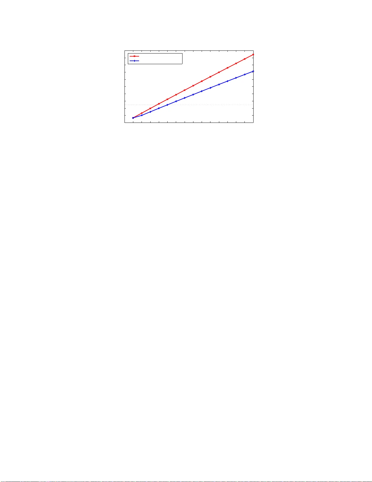
1 Precisely V erifying the Null Space Conditions in Compressed Sensing: A Sandwiching Algorithm Myung Cho and W eiyu Xu Abstract The null space condition of sensing matrices plays an important role in guaranteeing the success of compressed sensing. In this paper , we propose new ef ficient algorithms to v erify the null space condition in compressed sensing (CS). Giv en an ( n − m ) × n ( m > 0 ) CS ma trix A and a positi ve k , we are interested in computing α k = max { z : Az =0 ,z 6 =0 } max { K : | K |≤ k } k z K k 1 k z k 1 , where K represents su bsets of { 1 , 2 , .. ., n } , a nd | K | is the cardinality of K . In particular , we are interested in finding the maximum k such that α k < 1 2 . Howe ver , comp uting α k is kno wn to be extremely challenging. In this paper , we first propose a series of new polynomial-time algorithms to compute upper bounds on α k . Based on these ne w polynomial-time algorithms, we further design a new sandwiching algorithm, to compute the exact α k with greatly reduced complexity . W hen needed, this ne w sandwiching algorithm also achiev es a smoo th tradeof f between computation al complexity and result accuracy . Empirical results show the performance improv ements of our algorithm over existing kno wn methods; and our algorithm outputs precise value s of α k , with much lowe r complexity than exhausti ve search. Index T erms Compressed sensing, verifying the null space condition, the null space condition, ℓ 1 minimization I . I N T R O D U C T I O N In comp ressed sensing , a sensing m atrix A ∈ R ( n − m ) × n with 0 < m < n is g i ven, and we have y = Ax , where y ∈ R n − m is a measuremen t r esult and x ∈ R n is a signal. The spar est solution x to the underd etermined equ ation y = Ax is gi ven by (I .1): min k x k 0 subject to Ax = y (I.1) Myung Cho and W eiyu Xu are with the Department of Electrical and Computer Engineering, Uni versity of Iowa , Iow a City , IA, 52242 USA e-mail: myung-cho@u io wa.edu, weiyu-xu@uio wa.edu. 2 When the vector x has only k non zero elemen ts ( k -sparse signal, k ≪ n ), th e solution of ( I.2), wh ich is called ℓ 1 minimization , coincid es with th e solution of ( I.1) under certain co nditions, such as r estricted isometry conditions [1]–[6]. min k x k 1 subject to Ax = y (I.2) In orde r to gua rantee that we c an recover the sparse sign al by solv ing ℓ 1 minimization , we need to chec k these condition s ar e satisfied. The n ecessary an d sufficient cond ition f or the solutio n of (I .2) to coincide w ith th e solution of (I.1) is th e n ull space con dition (N SC) [7], [ 8]. Namely , when the NSC h olds for a numb er k , th en any k - sparse signal x can be e x actly r ecovered by solvin g ℓ 1 minimization . This NSC is defined as f ollows. Giv en a m atrix A ∈ R ( n − m ) × n with 0 < m < n , || z K || 1 < || z K || 1 , (I.3) ∀ z ∈ { z : Az = 0 , z 6 = 0 } , ∀ K ⊆ { 1 , 2 , ...n } w ith | K | ≤ k , where K is an ind ex set, | K | is the card inality o f K , z K is the elements of z vector correspo nding to the index set K , and K is the complement o f K . α k is defined as b elow , an d α k should be sm aller than 1 2 in order to satisfy the NSC. α k = max { z : Az =0 ,z 6 =0 } max { K : | K |≤ k } k z K k 1 k z k 1 A smaller α k generally mean s more robustness in recovering approximately sparse signal x via ℓ 1 minimization [7]–[9]. When a matrix H ∈ R n × m , n > m , is th e basis of the null space of A ( AH = 0 ), then the p roperty (I.3) is equiv a lent to the following prop erty (I.4): k ( H x ) K k 1 < k ( H x ) K k 1 , (I.4) ∀ x ∈ R m , x 6 = 0 , ∀ K ⊆ { 1 , 2 , ...n } w ith | K | ≤ k , where K is an index set, | K | is the car dinality o f K , ( H x ) K is the elements of ( H x ) correspo nding to the index set K , and K is the comp lement of K . (I.4) h olds if an d o nly if th e optimum value of (I. 5) is smaller th an 1. W e define the op timum value of (I.5) as β k : β k = max x ∈ R m , | K |≤ k k ( H x ) K k 1 subject to k ( H x ) K k 1 ≤ 1 . (I.5) And then α k is rewritten a s below: α k = max { x ∈ R m ,x 6 =0 } max { K : | K |≤ k } k ( H x ) K k 1 k ( H x ) k 1 = β k 1 + β k . W e a re interested in computing α k , and particularly finding the maxim um k such that α k < 1 2 . 3 Howe ver, solving the p rogram ming ( I.5) is difficult, because there are at least  n k  subsets K , which can be exponentially large in n and k , and the objective f unction is no t a conc a ve fu nction. I n fact, [10] sh ows th at g i ven a matrix A and a numb er k , com puting α k is strongly NP-hard. Unde r th ese computation al difficulties, testing the NSC w as o ften condu cted by ob taining an up per or lo wer bound on α k [2], [7], [11]–[13]. In [2] and [12], semidefinite r elaxation methods were intro duced by transfor ming the NSC into semidefinite pr ogrammin g to obtain the boun ds on α k or related q uantities. In [7] and [ 11], linear pro gramming (LP) relaxations were intro duced to obtain the upper and lower bounds on α k . Those papers s howed co mputable performance g uarantees on sparse signal rec overy with boun ds on α k . H owe ver , the bo unds resulting from [2], [ 7], [1 1]–[13], did not provide th e exact value of α k , which led to a small k v alue satisfying th e null space conditions. In this paper, we first propose a series of new polynomial- time algor ithms to comp ute u pper bounds on α k . Based o n these new po lynomial- time algorithm s, we further d esign a new sand wiching algorithm , to compute the exact α k with gr eatly red uced complexity . Th is new sandwich ing algorithm also offers a n atural way to ach iev e a smooth tradeoff b etween co mputational c omplexity an d result accura cy . By comp uting the exact α k , we ob tained bigger k values tha n results fro m [2 ] and [7]. This paper is organized as follows. In Section II, we provid e th e pick- 1 - element algorithm and a pro of showing that the p ick- 1 -eleme nt a lgorithm provides an u pper bound on α k . In Sectio n III, we provide the pick- l -element algorithm s, 2 ≤ l ≤ k , and a proof sho wing that the pick- l -eleme nt algo rithms also provide u pper bo unds o n α k . In Section IV, we con sider the pick- l -elemen t alg orithms with optim ized coefficients, 1 ≤ l ≤ k , and a p roof showing th at when l is incr eased, upp er bound on α k from the pick- l -elem ent algorith m with op timized c oefficients becomes smaller or stays the sam e. In Section V, we propose a sandwiching algorithm based o n the p ick- l -element algorithm s to o btain th e exact α k . In Sec tion VI and VI I, we pr ovide empirical r esults showing that th e improved perfor mance of our algor ithm o ver existing methods and conclude our paper by discussing e xtensions and future directions. I I . P I C K - 1 - E L E M E N T A L G O R I T H M Giv en a matrix H ∈ R n × m , 0 < m < n , in order to v erify α k < 1 2 , we pr opose a poly nomial-time alg orithm to find an upp er bo und on α k . Let us define α 1 , { i } as β 1 , { i } 1+ β 1 , { i } and β 1 , { i } as below: β 1 , { i } = max x ∈ R m k ( H x ) { i } k 1 subject to k ( H x ) { i } k 1 ≤ 1 , (II.1) where ( H x ) { i } is th e i -th ele ment in ( H x ) an d ( H x ) { i } is th e r est elements in ( H x ) . The su bscript 1 in β 1 , { i } is used to re present on e element and th e { i } in β 1 , { i } is used to rep resent the i -th ele ment in ( H x ) . The pick - 1 -elemen t algorithm is g i ven as follows to compu te an upper b ound on α k . 4 Algorithm 1: Pick - 1 -elemen t Algorithm for c omputing an u pper boun d on α k in Pseudo code Input : H matrix 1 for i = 1 to n do 2 β 1 , { i } ← outp ut of (II. 1) 3 α 1 , { i } ← β 1 , { i } / (1 + β 1 , { i } ) 4 Sort α 1 , { i } , i = 1 , ..., n , in descending order : α 1 , { i j } , j = 1 , ..., n 5 Compu te an upper bo und from the follo win g equatio n k X j =1 α 1 , { i j } 6 if u pper bou nd < 1 2 then 7 NSC is s atisfied Algorithm 2: Pick - 1 -elemen t Algorithm for c omputing an u pper boun d on α k in descr iption 1 Given a m atrix H , find an o ptimum value of (II.1): β 1 , { i } , i = 1 , 2 , ..., n . 2 Compu te α 1 , { i } with the values from Step 1 : α 1 , { i } = β 1 , { i } 1+ β 1 , { i } , i = 1 , 2 , ..., n 3 Sort these n d ifferent values o f α 1 , { i } in descendin g or der: α 1 , { i 1 } , α 1 , { i 2 } , ..., α 1 , { i n } , where α 1 , { i 1 } ≥ α 1 , { i 2 } ≥ ... ≥ α 1 , { i n } 4 Compu te th e sum of the first k values of α 1 , { i j } : P k j =1 α 1 , { i j } 5 If the result fr om Step 4 is sm aller 1 2 , then the null space con dition is satisfied. Lemma 2.1: α k can n ot be larger than th e sum of the k lar gest α 1 , { i } . Namely , α k ≤ k X j =1 α 1 , { i j } , where α 1 , { i 1 } ≥ α 1 , { i 2 } ≥ ... ≥ α 1 , { i k } ≥ ... ≥ α 1 , { i n } , i 1 , i 2 , ..., i k , ..., i n ∈ { 1 , 2 , ..., n } , and i a 6 = i b if a 6 = b . The subscrip t j of i j in α 1 , { i j } is u sed to represent that the values are sorted . Pr oof: W e assume that when x = x i , i = 1 , 2 , 3 , ..., n , we achieve the optimum value α 1 , { i } (= β 1 , { i } 1+ β 1 , { i } ) . Namely , β 1 , { i } = max x ∈ R m k ( H x ) { i } k 1 subject to k ( H x ) { i } k 1 ≤ 1 5 And we as sume that when x = x ∗ , we ach ie ve th e o ptimum value α k (= β k 1+ β k ) . β k = max x ∈ R m , | K |≤ k k ( H x ) K k 1 subject to k ( H x ) K k 1 ≤ 1 The inequ ality in Lemma 2.1 is th e sam e as th e following ( II.2): k ( H x ∗ ) K k 1 k ( H x ∗ ) k 1 | {z } | K | ≤ k ≤ k X j =1 k ( H x i j ) { i j } k 1 k ( H x i j ) k 1 , (II.2) (II.2) can b e rewritten as (II.3). X i ∈ K k ( H x ∗ ) { i } k 1 k ( H x ∗ ) k 1 ≤ k X j =1 k ( H x i j ) { i j } k 1 k ( H x i j ) k 1 (II.3) The left-ha nd side o f (II.3) can not be larger than t he sum of the α 1 , { i } , which is the max imum value for th e i -th element. X i ∈ K k ( H x ∗ ) { i } k 1 k ( H x ∗ ) k 1 ≤ X i ∈ K k ( H x i ) { i } k 1 k ( H x i ) k 1 | {z } α 1 , { i } maximum value of the i -t h element The sum of α 1 , { i } , i ∈ K , can not b e larger than the sum of the k largest α 1 , { i j } , j = 1 , 2 , ..., k . X i ∈ K k ( H x i ) { i } k 1 k ( H x i ) k 1 | {z } maximum value of 1 element in a set K ≤ k ( H x i 1 ) { i 1 } k 1 k ( H x i 1 ) k 1 | {z } 1st max. value of 1 element + ... + k ( H x i k ) { i k } k 1 k ( H x i k ) k 1 | {z } k -th max. value of 1 element I I I . P I C K - l - E L E M E N T A L G O R I T H M S In o rder to obtain b etter bou nds on α k than th e pick- 1 -element algorith m, in this section we genera lize the pick- 1 - element alg orithm to the pick- l -ele ment algo rithms, wher e l ≥ 2 is a fixed chosen integer no bigg er than k . The basic idea is to first compute the maximum portion max x ∈ R m k ( H x ) L k 1 k ( H x ) k 1 for ev ery subset L ⊆ { 1 , 2 , .., n } with cardinality | L | = l . On e c an then gar ner th is inform ation to ef ficiently comp ute an upper bound on α k . W e first ind ex the  n l  subsets with card inality l by indices 1 , 2 ,..., and  n l  ; and we deno te the subset correspon ding to ind ex i a s L i . Let us define β l,L i , i ∈ { 1 , 2 , 3 , ...,  n l  } , as: β l,L i = max x ∈ R m k ( H x ) L i k 1 subject to k ( H x ) L i k 1 ≤ 1 (III.1 ) The sub script l in β l,L i is used to denote the card inality l of the set L i , a nd i in β l,L i is the index of L i . T he pick- l -eleme nt algorithm in p seudocod e and in description are respecti vely listed as follo ws. 6 Algorithm 3: Pick - l -element Algo rithms, 2 ≤ l ≤ k for computing upp er b ounds on α k in Pseudo code Input : H matrix 1 for i = 1 to  n l  do 2 β l,L i ← outp ut of (III.1) 3 α l,L i ← β l,L i / (1 + β l,L i ) 4 Sort α l,L i , i = 1 , ...,  n l  in descen ding order : α l,L i j , j = 1 , ...,  n l  5 Compu te an upper bo und from the follo win g equatio n  1  k − 1 l − 1   ( k l ) X j =1 α l,L i j  6 if u pper bou nd < 1 2 then 7 NSC is s atisfied Algorithm 4: Pick - l -element Algo rithms, 2 ≤ l ≤ k for computing upp er b ounds on α k in descr iption 1 Given a m atrix H , find an o ptimum value of (III.1 ) : β l,L i , i ∈ { 1 , 2 , ...,  n l  } . 2 Compu te α l,L i from β l,L i : α l,L i = β l,L i 1+ β l,L i , i = 1 , 2 , ...,  n l  . 3 Sort these  n l  different values of α l,L i in descendin g or der : α l,L i j , wher e j = 1 , 2 , ...,  n l  and α l,L i a ≥ α l,L i b when a ≤ b . 4 Compu te th e sum of the first  n l  values of α l,L i j and divide the sum with (  k − 1 l − 1  ) :  1  k − 1 l − 1   ( k l ) X j =1 α l,L i j  5 If the result fr om Step 4 is sm aller than 1 2 , then the null space con dition is satisfied. The following lemma establishes an upp er bo und on α k . Lemma 3.1: α k can n ot be larger than th e output of the pick - l -element algo rithms, where 2 ≤ l ≤ k . Namely , α k ≤  1  k − 1 l − 1   ( k l ) X j =1 α l,L i j  | {z } upper bound calculated with the pick- l -element algorithm , where i j ∈ { 1 , 2 , 3 , ...,  n l  } ( 1 ≤ j ≤  n l  ) are  n l  distinct nu mbers; and α l,L i 1 ≥ α l,L i 2 ≥ ... ≥ α l,L i ( n l ) . Pr oof: Sup pose that the max imum value o f the pr ogrammin g (I. 5), namely β k , is ach ie ved when K = K ∗ . Let L ∗ i , 1 ≤ i ≤  k l  , be the family of s ubsets of K ∗ , with cardinality l . It is not har d to see that ea ch elemen t o f 7 K ∗ appears in  k − 1 l − 1  such subsets. In particu lar , we have K ∗ = ( k l ) [ i =1 L ∗ i . Thus, ∀ x ∈ R m , we can represent k ( H x ) K ∗ k 1 k ( H x ) k 1 as follows. k ( H x ) K ∗ k 1 k ( H x ) k 1 =  1  k − 1 l − 1   ( k l ) X i =1 k ( H x ) L ∗ i k 1 k ( H x ) k 1  (III.2 ) Suppose that each term of the rig ht-hand side of (III.2), k ( H x ) L ∗ i k 1 k ( H x ) k 1 , achieves the m aximum v alu e when x = x i ∗ , i = 1 , ...,  k l  ; and th e maxim um value of k ( H x ) K ∗ k 1 k H x k 1 in (I II.2) is achieved when x = x ∗ . Then, ∀ x ∈ R m , we ha ve k ( H x ) K ∗ k 1 k ( H x ) k 1 =  1  k − 1 l − 1   ( k l ) X i =1 k ( H x ) L ∗ i k 1 k ( H x ) k 1  , ∀ x ∈ R m ≤  1  k − 1 l − 1   ( k l ) X i =1 k ( H x i ∗ ) L ∗ i k 1 k ( H x i ∗ ) k 1  . (III.3 ) In the meantime, the m aximum outpu t f rom the pick- l -ele ment algor ithm is  1  k − 1 l − 1   ( k l ) X j =1 k ( H x i j ) L i j k 1 k ( H x i j ) k 1  , j = 1 , ...,  k l  . By our definitions of indices i j ’ s, we h av e  1  k − 1 l − 1   ( k l ) X i =1 k ( H x i ∗ ) L ∗ i k 1 k ( H x i ∗ ) k 1  ≤  1  k − 1 l − 1   ( k l ) X j =1 k ( H x i j ) L i j k 1 k ( H x i j ) k 1  . (III.4 ) Combining (II I.3), an d (III.4) lead s to k ( H x ∗ ) K k 1 k ( H x ∗ ) k 1 ≤  1  k − 1 l − 1   ( k l ) X j =1 k ( H x i j ) L i j k 1 k ( H x i j ) k 1  . Therefo re, we h a ve fin ished proving this lemm a. I V . P I C K - l - E L E M E N T A L G O R I T H M S W I T H O P T I M I Z E D C O E FFI C I E N T S The pick - l -element algorithm has 1 ( k − 1 l − 1 ) as its co efficients. In this section, we show that we can actually streng then the up per bound s of the pick- l -elem ent algorith ms, at the cost o f addition al p olynom ial-time complexity . In fact, we can calcu late i mproved upper b ounds on α k , using the pic k- l -e lement algorithm with optimized coefficients . Fro m this new alg orithm, we ca n show when l is in creased, the up per bound on α k becomes smaller o r stays the same. The upp er bo und from the pick- l - element algorithm is gi ven by  1  k − 1 l − 1   ( k l ) X j =1 α l,L i j  , (IV .1) 8 where α l,L i j , j = 1 , ...,  n l  are sor ted in descend ing o rder . The upp er bo und from the pick- l -e lement algor ithm with o ptimized coefficients is ob tained by solving th e following pr oblem: max γ i , 1 ≤ i ≤ ( n l ) ( ( n l ) X i =1 γ i α l,L i ) subject to γ i ≥ 0 , 1 ≤ i ≤  n l  , ( n l ) X i =1 γ i ≤ k l , X { i : I ⊆ L i , 1 ≤ i ≤ ( n l ) } γ i ≤  k − b l − b   k − 1 l − 1  , f or all integer s b such that 1 ≤ b ≤ l, f or all subsets I w ith | I | = b . (IV .2) Lemma 4.1: The pick- l - element algorithm with optim ized coefficients provides tighter , or at least the same, uppe r bound than the pick- l - element algo rithm. Pr oof: W e ca n easily see th at the fo llowing optim ization problem (I V .3) provides the same resu lt as th at fro m the pick - l -element algor ithm: max γ i , 1 ≤ i ≤ ( n l ) ( ( n l ) X i =1 γ i α l,L i ) subject to 0 ≤ γ i ≤ 1  k − 1 l − 1  , 1 ≤ i ≤  n l  , ( n l ) X i =1 γ i ≤ k l . (IV .3) And th is optimization prob lem (IV .3) is a relax ation of the pic k- l -element algorith m with optimized coefficients (IV .2). Ther efore, the p ick- l -element algorithm with optimized coefficients provides tighter , or a t least th e sam e, upper bou nd th an the pick- l - element algo rithm. Lemma 4.2: The pick- l -eleme nt algorithm with optim ized coefficients p rovide tig hter , o r at least the same, upper bound s than th e p ick- a -eleme nt algorithm with optimized co efficients when l > a . Pr oof: Fro m Lemma 5. 1, we ha ve α k,K ≤  1  k − 1 l − 1   ( k l ) X i =1 α l,L i  | {z } upper bound of k elements calculated with the pick- l -element algorithm , 1 ≤ l ≤ k , 9 where L i , 1 ≤ i ≤  k l  , are all the subsets of K with car dinality l . W e c an up per b ound ( IV .2) by the f ollowing: max γ i , 1 ≤ j ≤ ( n l ) ( ( n l ) X i =1 γ i 1  l − 1 a − 1  X { j : A j ⊂ L i , | A j | = a } α a,A j ) subject to γ i ≥ 0 , 1 ≤ i ≤  n l  , ( n l ) X i =1 γ i ≤ k l , X { i : I ⊆ L i , 1 ≤ i ≤ ( n l ) } γ i ≤  k − b l − b   k − 1 l − 1  , f or all integer s b such that 1 ≤ b ≤ l, f or all subsets I with | I | = b . (IV .4) (In the objective function o f (IV .4 ), each α a,A j , 1 ≤ j ≤  n a  appears  n − a l − a  times.) B y definin g 1 ( l − 1 a − 1 ) P { i : A j ⊂ L i , 1 ≤ i ≤ ( n l ) } γ i as γ ′ j and relax ing (I V .4), we can obtain (IV .5) wh ich is the same a s the pick- a -element alg orithm with op timized coefficients. max γ ′ j , 1 ≤ j ≤ ( n a ) ( ( n a ) X j =1 γ ′ j α a,A j ) subject to γ ′ j ≥ 0 , 1 ≤ j ≤  n a  , ( n a ) X j =1 γ ′ j ≤ k a , X { j : I ⊆ A j , 1 ≤ j ≤ ( n a ) } γ ′ j ≤  k − b a − b   k − 1 a − 1  , f or all integers b such that 1 ≤ b ≤ a, f or all subse ts I w ith | I | = b . (IV .5) In fact, the first, second, and third constraints of (IV .5) ca n be obtained from the relaxation of the constraints of (IV .4). The first constraint of (IV .5) is t rivial. Th e second con straint of (IV .5) is from the follo wing: ( n a ) X j =1 γ ′ j = ( n a ) X j =1 1  l − 1 a − 1  X { i : A j ⊂ L i , 1 ≤ i ≤ ( n l ) } γ i = 1  l − 1 a − 1   l a  ( n l ) X i =1 γ i ≤ 1  l − 1 a − 1   l a  k l = k a 10 The third c onstraint of ( IV .5) co mes from the f ollowing: X { j : I ⊆ A j , 1 ≤ j ≤ ( n a ) , | I | = b } γ ′ j = X { j : I ⊆ A j , 1 ≤ j ≤ ( n a ) , | I | = b } 1  l − 1 a − 1  X { i : A j ⊂ L i , 1 ≤ i ≤ ( n l ) } γ i = 1  l − 1 a − 1   n − b a − b  n − a l − a   n − b l − b  X { i : I ⊂ L i , 1 ≤ i ≤ ( n l ) , | I | = b } γ i ≤ 1  l − 1 a − 1   n − b a − b  n − a l − a   n − b l − b   k − b l − b   k − 1 l − 1  , 1 ≤ b ≤ a =  k − b a − b   k − 1 a − 1  , 1 ≤ b ≤ a Because (IV .5) is o btained fr om the r elaxation of (IV .4), the optimal value of (IV .5) is larger or equal to the o ptimal value of ( IV .4), and (IV .5) is nothin g but the pick- a -element alg orithm with optimized coe ffi cients. Th erefore, the pick- l -eleme nt algorithm provides tighter, or at least the same, up per bo unds than th e pick- a -element algo rithm with op timized co efficients, when l > a . V . T H E S A N D W I C H I N G A L G O R I T H M From Section II, Section III and Section IV, we ha ve upp er bounds on α k with the pick- l -element algorithm, 1 ≤ l ≤ k : α k ≤  1  k − 1 l − 1   ( k l ) X j =1 α l,L i j  | {z } upper bound calculated with the pick- l -element algorithm , or th e p ick- l -element algorithm with optimized coef ficients, 1 ≤ l ≤ k . Howe ver, these alg orithms do not p rovide the exact value f or α k . In order to obtain th e exact value, rather th an up per b ounds on α k , we devise a sand wiching algorithm with g reatly reduced com putational complexity . W e remar k that the conve x pr ogrammin g method s in [ 2] and [7] only provide upp er b ounds on α k , instead o f exact values of α k , except when k = 1 . The idea o f ou r sandwiching algorith m is to maintain two b ounds in com puting the exact value of α k : an u pper bound on α k , and a lower b ound on α k . In algor ithm e xecutio n, we con stantly decrease the upper bound, and increase th e lower bou nd. Wh en the lower bound and upper bo und meet, we immed iately get a certification that the exact value of α k has been reac hed. There are two ways to compute the up per b ounds: the ‘ cheap’ upper bou nd and the linear program ming based upper boun d. Th ese two up per b ounds are stated in Le mmas 5.1 and 5.2 re specti vely . Lemma 5.1 ( ‘cheap’ up per bound ): Gi ven a set K with car dinality k , we ha ve α k,K ≤  1  k − 1 l − 1   ( k l ) X i =1 α l,L i  | {z } upper bound of k elements calculated with the pick- l -element algorithm , 1 ≤ l ≤ k , (V .1) 11 where α k,K = β k,K 1+ β k,K and β k,K is defined as below , and L i , 1 ≤ i ≤  k l  , are all the subsets of K with car dinality l . β k,K = max x ∈ R m k ( H x ) K k 1 subject to k ( H x ) K k 1 ≤ 1 (V .2) ( β k,K is de fined for a given K set with cardinality k , but β k is the maximu m value over a ll subsets with c ardinality k .) Pr oof: T his pro of follows the same reasonin g a s in Lemma 3. 1. Let L i , 1 ≤ i ≤  n l  , be the family of su bsets of K , with cardinality l . It is not har d to see that ea ch element of K appear s in  k − 1 l − 1  such subsets. In p articular, we have K = ( k l ) [ i =1 L i . Thus, ∀ x ∈ R m , we can represent k ( H x ) K k 1 k ( H x ) k 1 as follows. k ( H x ) K k 1 k ( H x ) k 1 =  1  k − 1 l − 1   ( k l ) X i =1 k ( H x ) L i k 1 k ( H x ) k 1  (V .3) Suppose that each term of the r ight-han d side of (V .3), k ( H x ) L i k 1 k ( H x ) k 1 , achiev es th e m aximum value when x = x i , i = 1 , ...,  k l  ; and th e maxim um value of k ( H x ) K k 1 k H x k 1 in (V .3) is achie ved when x = x ∗ . The n, we ha ve k ( H x ∗ ) K k 1 k ( H x ∗ ) k 1 =  1  k − 1 l − 1   ( k l ) X i =1 k ( H x ∗ ) L i k 1 k ( H x ∗ ) k 1  ≤  1  k − 1 l − 1   ( k l ) X i =1 k ( H x i ) L i k 1 k ( H x i ) k 1  . W e can also obtain the up per bou nd on α k,K on a given K set by solvin g the following optimiza tion prob lem (V .4): max ( k X j =1 z j ) subject to X t ∈ L i z t ≤ α l,L i , ∀ L i ⊆ K with | L i | = l, i =1 ,..., ( k l ) , z j ≥ 0 , j = 1 , 2 , ..., k . (V .4) Lemma 5.2 ( linear pr ogramming based up per bound ): The optimal o bjectiv e value of (V .4) is an upper bound on α k,K . 12 Pr oof: By the definitio n of β k,K , we can write α k,K (= β k,K 1+ β k,K ) as the optima l objective value of the fo llowing optimization pro blem. max x ∈ R m k ( H x ) K k 1 k ( H x ) k 1 subject to k ( H x ) L i k 1 k ( H x ) k 1 ≤ β l,L i 1 + β l,L i , i = 1 , ...,  k l  . (V .5) This is because, b y the definition of β l,L i , the n ewly ad ded co nstraints k ( H x ) L i k 1 k ( H x ) k 1 ≤ β l,L i 1+ β l,L i , i = 1 , ...,  k l  , ar e ju st redund ant constraints which always hold tr ue over x ∈ R m . Represen ting z t = k ( H x ) { t } k 1 k ( H x ) k 1 , t = 1 , ..., n , we can relax (V .5) to (V .4). Thu s th e optima l objective value o f (V .4) is an up per b ound on tha t of (V .5), namely α k,K . Lemma 5.3: The optimal obje cti ve value f rom (V .4) is no larger than th at of (V .1). Pr oof: Sum ming up the constraints in (V .4) X t ∈ L i z t ≤ α l,L i | {z } Exact value of l elements , ∀ L i ⊆ K with | L i | = l, i =1 ,..., ( k l ) , we get th e numb er in (V .1), since each element in K appears in  k − 1 l − 1  subsets of ca rdinality of l . In Algorithms 5 and 6, we shows how we implemen ted the sandwiching alg orithm. Th e fo llowing theorem claims that Algo rithms 5 and 6 will o utput the exact value of α k in a finite num ber o f steps. Theor em 5.4: The glo bal lower and upper bo unds on α k will both con verge to α k in a finite number of steps. Pr oof: In the san dwiching a lgorithm, we fi rst use the p ick- l -elemen t algo rithm to calcu late the values of α l,L for every sub set L with c ardinality l . T hen using the ‘cheap ’ upper bo und (V .1), we calculate the u pper boun ds o n α k,K for ev ery set K with car dinality k . W e then sort these subsets in descending o rder by their u pper bo unds. In algorithm e xecution, bec ause o f sorting, the glob al u pper bound GUB on α k never r ises. In th e meanwhile, the glob al lower bou nd GLB either rises or stays un changed in each iteration. If the algorithm comes to an index i , 1 ≤ i ≤  n k  , s uch that th e upp er bound of α k,K i for the i -th sub set K i is alre ady smaller than the global lower bound GLB, the algorithm will make the g lobal u pper boun d GUB equal to th e glob al lower b ound GLB. A t th at moment, we know th ey must bo th be equ al to α k . This is b ecause, from the descending o rder of the upp er bounds on α k,K , each subset K j with j > i must ha ve an α k,K j that is sm aller than the glo bal lower b ound GLB. In the meanwhile, as specified by the sand wiching algorithm, the glo bal lo wer boun d GLB is the largest amo ng α k,K j with 1 ≤ j ≤ ( i − 1) . So a t this point, the GLB must be the largest among α k,K j with 1 ≤ j ≤  n k  , namely GLB = α k . If we can no t find such an ind ex i , the algorithm will end up calcu lating α k,K for every set K in th e list. In this case, the u pper and lower boun d will als o be come e qual to α k , after each α k,K has been calculated. A. Calculating α k,K for a set K The exact value of α k,K (= β k,K 1+ β k,K ) is calculated by solvin g (V .2) for a subset K . However , the objective function is not concave. In order to solve it, we sep arate the ℓ 1 norm of ( H x ) K into 2 k possible cases accordin g to the sign 13 Algorithm 5: San dwiching A lgorithm for co mputing exact value of α k in Pseudo co de / * Global Upper Bound: GUB * / / * Global Lower Bound: GLB * / / * Cheap Upper Bound: CUB * / / * Linear Programming based Upper Bound: LPUB * / / * Local Lower Bound: LLB * / Input : Sets L j with | L j | = l , and α l,L j correspond ing to L j , j = 1 , ...,  n l  1 Compute the CUB on α k,K for all the subsets K with | K | = k . 2 Sort these subsets in descending order of their CUB 3 Initiali ze GLB ← 0 4 for i = 1 to  n k  do 5 if GLB < the CUB of the i -th sorted subset K i then 6 GUB ← the CUB of the i -th sorted subset K i 7 LPUB ← the upper bound on α k,K i from (V . 4) for the i -th subset K i 8 if GLB < LPUB then 9 LLB ← α k,K i , after computing α k,K i . 10 if LLB > GLB then 11 GLB ← LLB 12 end 13 end 14 else 15 GUB ← GLB 16 break 17 end 18 end 19 GUB ← GLB; 20 if GUB < 1 2 then 21 NSC is satisfied 22 else 23 NSC is not satisfied 24 end of ea ch term, +1 or − 1 . Hence, w e can make a ℓ 1 optimization pro blem into 2 k small lin ear pr oblems. For eac h possible case, we find the m aximum can didate value fo r β k,K via the f ollowing: max x ∈ R m X i ∈ K sign i ∈{− 1 , 1 } sig n i × ( H x ) { i } subject to k ( H x ) K k 1 ≤ 1 , (V . 6) where sig n i is for the sign of i -th term. I n fact, we d o not need to calculate 2 k small linear problems. W e o nly need to calculate 2 k − 1 problem s instead of 2 k , because the re sult fr om (V .6) for on e p ossible case (e.g. 1,-1 ,-1,1 when k = 4 ) o ut of 2 k cases is always equivalent to the r esult for its in verse case ( e.g. -1,1,1 ,-1). Amo ng th e 2 k − 1 candidates, we c hoose the big gest one as β k,K . This strategy is also ap plied to solve (II.1) an d (III.1). 14 Algorithm 6: San dwiching A lgorithm for co mputing exact value of α k in description * Global Upper Bound (GUB): the current upper bound α k * Global Lower Bound (GLB): the current lower bound for α k * Cheap U pper Bound (CUB): the upper bounds obtained from (V .1) * Linear Progra mming based Upper Bound (LPUB): the upper bounds obtained from (V .4 ) 1 For a fixed nu mber l < k , compute α l,L j , j = 1 , ...,  n l  , for all the subsets L j with | L j | = l . Compute th e cheap up per b ounds on α k,K for all s ubsets K with | K | = k , a nd sort th ese subsets by th eir chea p up per bound s in descending orde r . 2 Initialize GLB ← 0 and the index i ← 1 . 3 If i =  n k  + 1 , then assign GUB ← GLB and g o to Step 7. I f the CUB o f the i - th sorted subset is no bigger than than GL B, then assign GUB ← GLB an d go to Step 7. 4 Assign GU B ← the CUB of the i - th sorted subset K i , and com pute th e LPUB f or this sub set K i . 5 If the LPUB o f the i - th subset K i is bigge r than GLB, then calculate the exact α k,K i by solving (V .2) and assign GLB ← α k,K i only if α k,K i > GLB. 6 Incre ase th e in dex i ← ( i + 1) and go to Step 3. 7 If GUB is smaller than 1 2 , the n ull space co ndition is satisfied. If not, th e null spac e c ondition is no t satisfied. B. Computatio nal Complexity The san dwiching algo rithm consists of th ree majo r parts. The first part perfor ms th e p ick- l -element algorithm f or a fixed num ber l . The seco nd part is the comp lexity of co mputing the uppe r bo unds o n α k,K , and s orting the  n k  subsets K by the u pper bo unds on α k,K in descending orde r . T he third part is to exactly compute α k,K for each subset K , starting fr om th e top o f the sorted list, before the up per b ound m eets th e lower bou nd in the a lgorithm. The first part o f the san dwiching algo rithm c an be fin ished with poly nomial-time co mplexity , wh en the num ber l is fixed. The com plexity o f the seco nd par t grows exponentially in n ; h owe ver, co mputing the u pper bo unds based on the pick- l - element algorithm s, and r anking the up per bou nds are v er y ch eap in co mputation . So when n and k are not big (for example, n = 40 and k = 5 ), this second step can also be finished reasonably fast. W e r emark that, howe ver, when n and k are b ig, on e may enu merate these br anches one by one seque ntially , in stead of computin g and ranking them in one shot (A detailed discussion o f this is out of the scope of this curren t p aper). The main complexity then co mes from the th ird part, wh ich depen ds h eavily o n, for how many subsets K the algorithm will exactly com pute α k,K , before the upper bo und and the lo wer bound meet. In turn, this depends o n how tight the upper bou nd a nd lower b ound ar e in algo rithm execution. In th e worst case, the u pper and lower bo und can meet wh en  n k  subsets K have been e xamined . Howe ver , in practice, we find that, very o ften, th e up per bou nds and the lower bo unds meet very quickly , o ften way befo re the algorithm has to examin e  n k  subsets. Thus the algor ithm will ou tput th e exact value of α k , by using mu ch lower 15 computatio nal comp lexity than the exhaustive search method. Intu iti vely , subsets with bigger upp er b ounds on α k,K also tend to offer big ger exact values of α k,K . This in turn leads to very tigh t lower boun ds on α k . As we go down the sorted list of sub sets, the lower boun d becomes tighter and tig hter , while the u pper boun d also becom es tigh ter and tighter, since the u pper bounds were sorted in d escending order . Thus the lower and upp er bo unds can becom e equal very qu ickly . In the e xtreme case, if both upper and lo wer bound s are tight at the beginnin g, the sandwich algorithm will be ter minated at th e very first step. T o analy ze how quickly the upper and lower bound meet in this algorithm is a very inter esting pr oblem. V I . S I M U L A T I O N R E S U L T S W e con ducted simulations using Matlab on a HP Z220 CMT workstation with Intel Cor ei7-377 0 dua l core CPU @ 3.4GHz clock speed and 1 6GB DDR3 RAM, u nder Windo ws 7 OS environmen t. T o so lve op timization pr oblems such a s (I I.1), (III. 1), (V .2), and (V . 4), we used CVX, a package for specifying and solvin g co n vex progr ams [ 14]. T ables r anging from I to X are the r esults for Ga ussian matrix cases . Gau ssian matrix H was chosen r andomly and simulated for various k fro m 1 to 5. The elements of H matrix follow i.i.d. standard Gau ssian distribution N (0 , 1) . T able I, II and III show upper bounds on α k obtained f rom th e p ick- 1 -eleme nt algorithm, the pick- 2 -element algorithm , and the pick- 3 -element algorithm r espectiv ely for Gaussian matrix cases. W e ran simulations o n 10 different rand om m atrices H for eac h size and obtained med ian value of them. α 1 in T able II and III is from T able I and α 2 in T ab le III is from T ab le II. T able IV shows the exact α k from the sandwichin g algorithm on d ifferent sizes of H matrices and different values of k . W e ran simula tions on one random ly cho sen matrix H at each s ize. Henc e in total, we tested 4 different H matrices in this simulation (ou r simulation exper ience shows that the perfor mance a nd comp lexity of the sandwich algorithm c oncentrates fo r rand om matrices under this dimension). The pick- l -element algorith m mostly used in the sand wiching algor ithm is the p ick- 2 -elem ent algo rithm, except for α 2 in all H matrix cases, α 4 in the 40 × 2 0 H matrix case and α 5 in the 40 × 12 , 40 × 16 , and 40 × 20 H matrix cases. For α 2 in all H matrix cases, the sandwiching algo rithm based on th e pick- 1 -element alg orithm is used. For other exception al cases, the san dwiching algorithm based o n the pick- 3 -element a lgorithm is used, because of the fas ter runn ing tim e th an the sandwich ing algorithm based on the pick- 2 -elemen t algor ithm. Th e obtained e xact α k is in T able IV and the number of s teps and running tim e to r each th at exact α k are in T able VI and T able VII respectively . W e cited the results f rom [2] and [7] in T a ble V for easy co mparison with ou r results. The exact values α k from our algor ithm clear ly improve on th e u pper and lower boun ds from [2] an d [7]. W e added one m ore co lumn in T able V f or max imum k satisfying α k < 1 2 based on th eir results. In the 40 × 12 and 4 0 × 16 H matrix cases, we ha ve big ger k than [2] an d [7]. T able VI sho ws the n umber of ru nning steps to get the exact α k in T able IV, using ou r sandwiching algorith m. As shown in T able VI, we can r educe running steps con siderably in re aching the exact α k , compar ed with the exhaustiv e search meth od. When k = 3 , f or the 40 × 16 H matrix case, the number of running steps was r educed to abou t 1 700 of the steps in the exh austi ve searc h m ethod. The r unning steps fo r k = 4 and the same H matrix are 16 reduced to about 1 40 of th e steps in the exhausti ve searc h metho d. In k = 5 case, the reduction rate b ecame 1 5 on the same H matrix. W e think th at this is b ecause when k is big , the g ap between the u pper boun d on α k from th e pick- 2 - element algorithm , and the lower bou nd beco mes big, thu s the n umber o f ru nning step s is increased. (Wi th the sandwichin g algorithm based on the p ick- 3 -elem ent algorithm in k = 5 and the 40 × 16 H m atrix case, th e reduction rate b ecame 1 4400 .) T able VI I lists th e actual run ning time of the sandwichin g algo rithm (mostly based on the pick- 2 -element algorithm ). E xcept for k = 2 , the pick- 1 - element algorithm is used as the step s in the sand wiching algorithm. For k = 4 in the 40 × 2 0 H matrix case, a nd k = 5 in the 4 0 × 1 2 , 40 × 16 and 40 × 12 cases, the pick- 3 -element algorithm is used in the sandwiching algorithm. F or k = 5 in the 40 × 20 H matrix, our sandwiching algorithm finds the exact value using on ly 1 170 of th e time u sed by the exhau sti ve search meth od: the sandwichin g algorith m takes around 2 . 2 ho urs, while the exhaustive sear ch method will take aroun d 16 da ys to find the exact value of α k . T able VIII shows the estimated runn ing time of the e x haustive search method. In o rder to estimate the running time, we measured the runnin g time to obtain α k,K for 100 rand omly chosen sub sets K with | K | = k , and calculated the average time spent p er subset. W e m ultiplied th e time per s ubset with the n umber of subsets in th e exhaustiv e search method to calculate the overall ru nning time of the e x haustiv e search method. For k = 1 case, we put the actual oper ation time from T able VII. T ables ranging from XI to XVII are the results for Fourier matrix cases and T ables ranging from XVIII to X XIV are the results for B ernou lli matr ix cases. F or F ourier m atrix cases and Bernoulli ma trix cases, we u sed A matrix in simulations in stead of its nu ll space matr ix. A matr ix was chosen r andomly and simulated fo r various k from 1 to 5. T able XI, T able X II, and T able XIII show u pper boun ds on α k for Fourier matrix ca ses. W e ran si mulations o n 10 d ifferent rando m Fourier matrices for each size and obtained median value o f them. α 1 in T ab le XI I and XIII is from T ab le XI and α 2 in T ab le XIII is from T ab le XII. T able XIV shows the exact α k from the san dwiching algorithm on different sizes o f F o urier matrices A and different values o f k . W e ran simulations o n one ran domly chosen Fourier matrix A at each size. Hence in total, we tes ted 4 different Fourier matrices in this simulation. The obtained exact α k via ou r sand wiching algo rithm is in T able XIV an d the number of steps and run ning time to reach that exact α k are in T able XV an d T able XVI respectively . The exact values α k from o ur algorithm clearly improve on the up per and lower bou nds from [2] an d [7] for F ou rier matrix ca ses as well. F or example, when our re sult f or α k is comp ared to the r esults from [2 ] an d [7] in 20 × 40 Fourier matrix, we obtained 0.6 7 for e x act α 5 , while b oth [2] and [ 7] p rovides 0.9 8 as their upper bound s on α 5 .) In T able XIV, th e p ick- l -element algorith m mostly used in the san dwiching alg orithm is the pick- 2 -element algorithm , except for α 2 , and α 5 in the 2 0 × 40 and 32 × 40 matrix cases. For α 2 , the sandwiching algorithm b ased on the pick- 1 -elem ent algor ithm is used. For α 5 in the 2 0 × 40 and 3 2 × 40 matrix cases, the san dwiching algorith m based on th e pick- 3 - element algor ithm is used, bec ause of the faster run ning time than the sandwiching algo rithm based on the pick- 2 - element algor ithm. In T ab le XV, when k = 2 , some results from the sandwichin g a lgorithm 17 based on the p ick- 1 -elem ent algo rithm r eached the maxim um o peration steps, nam ely  n k  steps. Th is is because in those Fourier matr ices, the upper boun ds ob tained fro m (V .1) and ( V .4) were to o weak to satisfy con ditions in t he progr am to stop the simu lation in the middle of the op eration early . T able XVIII, T able XI X, and T able XX show up per bound s on α k for Berno ulli matrix cases. W e r an simulations on 10 different rando m Bernoulli matrices for each size and ob tained media n value of them . α 1 in T able XIX and XX is fr om T able XVI II and α 2 in T able XX is from T ab le XIX. T able XXI shows th e exact α k from the san dwiching algorithm o n dif ferent si zes of Bernoulli m atrices A an d different values of k . W e ran simulations o n on e random ly chosen Berno ulli matrix A at each size. Hen ce in total, we tested 4 different Bernou lli matr ices in th is simulation. The obtained exact α k via our sandwichin g algor ithm is in T able XXI and th e nu mber of steps and run ning time to rea ch that exact α k are in T able XXII and T a ble XXII I respectively . In T able XXI, in or der to o btain α 2 , the pick- 1 -element alg orithm is used in the sandwiching algorithm ( the sandwiching algorithm ba sed on the pick - 1 -elemen t algorithm) . For α 5 in the 2 0 × 40 , 24 × 40 , an d 28 × 40 , the pick- 3 - element algorithm is used in th e sandwich ing algorithm (th e sandwich ing algorithm based on the pick- 3 - element algo rithm). When it co mes to comp aring the results fr om our sand wiching algorithm with the results from [2] and [7], we h av e b igger recoverable k in the 24 × 40 , 28 × 40 , and 3 2 × 40 Ber noulli matrix c ases. Figures 1, 2, and 3 show histograms of the san dwiching algorithm co nducted o n 100 exam ples 40 × 20 Gaussian matrices. T he sandwiching algo rithm based o n the pick- 3 -e lement algor ithm is used in our simu lations. The median value of α 5 , numbe r of steps and operation time of the sandwich ing algorithm in this 100 trials are respectively 0.73, 140 0 steps, and 9 5.36 minutes. T he data o f 10 samples out of 100 tr ials are in T able IX. W e remark that, if one attemp ts to use exhaustiv e search to get the exact α k for these 100 m atrices, it would take aro und 4 y ears on our mach ine. 0.7 0.72 0.74 0.76 0.78 0.8 0.82 0.84 0.86 0 5 10 15 20 25 30 exact α 5 number of samples Figure 1: Histog ram of the exact α 5 from the s andwichin g algorithm ( 4 0 × 20 Gaussian matrix ) Figure 4 shows how fast the upper boun d and lower bou nd ar e ap proachin g each o ther in th e san dwiching algorithm (based on the pick- 2 -elem ent algo rithm), for k = 5 and 40 × 20 H Gaussian matrix case. W e can see that, the sandwic hing algorithm offers a g ood tradeoff between result accuracy and comp utation complexity , if we ev e r want to terminate the algor ithm ear ly . Figure 5 is th e g raph for the up per b ound on α k versus k in 1 02 × 256 A Gaussian matrix, ( A ∈ R 102 × 256 ). W e 18 0 2000 4000 6000 8000 10000 12000 14000 16000 0 10 20 30 40 50 60 number of steps in the sandwiching algorithm number of samples Figure 2: Histogram of th e num ber o f steps in the sandwic hing algorithm ( 40 × 20 Gau ssian matrix) 80 100 120 140 160 180 200 220 0 10 20 30 40 50 60 70 operation time (min.) of the sandwiching algorithm number of samples Figure 3: Histog ram of op eration time in th e sandwiching algo rithm ( 40 × 20 Gaussian m atrix) 0 500 1000 1500 2000 2500 3000 3500 4000 4500 5000 0 0.1 0.2 0.3 0.4 0.5 0.6 0.7 0.8 0.9 Running Steps Bound Value Upper Bound Lower Bound Figure 4: Globa l Upp er Bound (GUB) and Glob al Lower Bound (GLB) in the sandwich ing alg orithm based on the pick- 2 - element algor ithm ( α 5 in the 4 0 × 20 H Gau ssian matrix case) obtained k = 5 ( α 5 = 0.49) f rom the pick - 2 -elemen t a lgorithm as maximum k su ch that α k < 1 / 2 in 102 × 256 Gaussian matrix, while [ 7] provide d 4 f or recoverable sparsity in a Gaussian matrix of the same dime nsion. ( α 1 in the pick - 2 -elemen t alg orithm comes fro m α 1 in the p ick- 1 -elem ent algorith m.) The d ata are in T able X . V I I . C O N CL U S I O N In this pap er , we propo sed new algor ithms to verify the null space con ditions. W e first pr oposed a series of new polyno mial-time algorithm s to compute upper bound s on α k . Based on these new polyn omial-time algorith ms, we further design ed a ne w sand wiching algorith m, to co mpute the exact α k with gr eatly red uced complexity . 19 0 1 2 3 4 5 6 7 8 9 10 11 12 13 14 15 0 0.2 0.4 0.6 0.8 1 1.2 1.4 1.6 1.8 2 2 k upper bound on α k pick−1−element algorithm pick−2−element algorithm Figure 5: Upper Bounds o n α k from th e pick- 1 -element algorithm and the pick- 2 - element alg orithm ( 102 × 25 6 A Gaussian matrix) The futur e work f or verifying th e null space cond itions includes designing ef ficient algorithms to reduce the operation time ev e n m ore. It is also interesting to extend the framework to th e nonlinear measurem ent setting [15]. R E F E R E N C E S [1] Emmanuel Cand ` es and T erence T ao, “ Decoding by linear programming, ” Information Theory , IEEE T ransact ions on , vo l. 51, no. 12, pp. 4203–4215, 2005. [2] Alexa ndre d’Aspremont and Laurent El Ghaoui, “T esting the nul lspace property using semide finite programming , ” Mathematic al pr ogramming , vol. 127, no. 1, pp. 123–144, 2011. [3] Emmanuel Cand ` es, Justin Romberg, and T erenc e T ao, “Robust uncertai nty principles: Exact signal recon struction from highly incomplet e frequenc y information, ” Inf orm ation Theory , IEE E Tr ansactions on , vol. 52, no. 2, pp. 489–509, 2006. [4] Emmanuel Cande s , Justin K Rombe rg, and T erence T ao, “Stable signal rec overy from incompl ete and ina ccurate measurements, ” Communicat ions on pur e and applie d mathematics , vol . 59, no. 8, pp. 1207–1223, 2006. [5] David Donoho, “Neighborly polytopes and sparse solution of underdetermine d linear equations, ” 20 05. [6] Benjamin Recht, W eiyu Xu, and Babak Hassibi, “Null space conditions and thresho lds for rank minimizati on, ” Mathematic al pr ogramming , vol. 127, no. 1, pp. 175–202, 2011. [7] Anatoli Juditsky and Arkadi Nemirovski, “On v erifiable suf ficient con ditions for sparse signal recovery via ℓ 1 minimizat ion, ” Mathemati cal pr ogramming , vol. 127, no. 1, pp. 57–88, 2011. [8] Albert Cohen, W olfgang Dahmen, and Ronald DeV ore, “Compressed sensing and best k -term approximation, ” Journal of the American Mathemat ical Socie ty , vol . 22, no. 1, pp. 211–231, 2009. [9] W eiyu Xu and Bab ak Hassibi, “Prec ise stability phase transiti ons for l1 minimiz ation: A unified geometr ic framew ork, ” IEEE transac tions on information theory , vol. 57, no. 10, pp. 6894–6919, 2011. [10] M. Pfetsch and A. T illmann, “The computation al complexi ty of the rest ricted isometry property , the nullspa ce property , and related concepts in compressed sensing, ” , 2012. [11] Gongguo T ang an d Arye Nehorai, “Perfo rmance analysis of sparse reco very base d on constrai ned m inimal singul ar v alues, ” IEEE T ransacti ons on Signal Pr ocessing , vol. 59, no. 12, pp. 5734–5745, 2011. [12] Gongguo T ang and Arye Nehora i, “V erifiable and computable ℓ ∞ performanc e ev aluation of ℓ 1 sparse signal reco very , ” arX iv:1102 .4868 , 2011. [13] Kiryung L ee and Y oram Bresler , “Computing performance guarantee s for compressed sensing, ” in IEEE Internation al Co nfer ence on Acoustics, Speec h and Signal Pr ocessing . IEEE , 2008, pp. 5129–5132. [14] Michae l Grant and Stephen Boyd, “CVX: Matlab software for discipline d con vex programming, versi on 2. 0 beta, ” http:/ /cvxr . com/cvx, Sept. 2012. 20 [15] W eiyu Xu, Meng W ang, Jianfe ng Cai, and Ao T ang, “Sparse recov ery from nonlinear measurements with applic ations in bad data detec tion for powe r netwo rks, ” , 2011. 21 T able I: Upper b ounds from the pick- 1 -element algo rithm ( Gaussian Matrix) (Rounded off to the nearest hundredth) H matrix(n × m) ρ a α 1 α 2 α 3 α 4 α 5 k b 40 × 20 0.5 0.27 0.54 0.79 1.03 1.27 1 40 × 16 0.6 0.23 0.44 0.65 0.86 1.06 2 40 × 12 0.7 0.19 0.36 0.53 0.70 0.86 2 40 × 8 0.8 0.15 0.29 0.43 0.56 0.69 3 a ρ = ( n − m ) /n b Maximum k s.t. α k < 1 / 2 T able II: Upper bounds fr om th e pick- 2 -element algor ithm (Ga ussian Matrix) (Rounded off to the nearest hundredth) H matrix(n × m) ρ a α 1 α 2 α 3 α 4 α 5 k b 40 × 20 0.5 0.27 0.46 0.65 0.83 1.02 2 40 × 16 0.6 0.23 0.37 0.53 0.69 0.85 2 40 × 12 0.7 0.19 0.32 0.46 0.60 0.73 3 40 × 8 0.8 0.15 0.25 0.37 0.48 0.59 4 a ρ = ( n − m ) /n b Maximum k s.t. α k < 1 / 2 T able III: Upp er bo unds from the pick- 3 -element algo rithm (Gaussian Matrix) (Rounded off to the nearest hundredth) H matrix(n × m) ρ a α 1 α 2 α 3 α 4 α 5 k b 40 × 20 0.5 0.27 0.46 0.55 0.72 0.88 2 40 × 16 0.6 0.23 0.37 0.47 0.61 0.74 3 40 × 12 0.7 0.19 0.32 0.41 0.54 0.65 3 40 × 8 0.8 0.15 0.25 0.33 0.43 0.52 4 a ρ = ( n − m ) /n b Maximum k s.t. α k < 1 / 2 22 T able IV : Exact α k from the s andwichin g algo rithm ( Gaussian Matrix) (Rounded off to the nearest hundredth) H matrix(n × m) ρ a α 1 α 2 c α 3 α 4 α 5 k b 40 × 20 0.5 0.27 0.42 0.54 0.63 d 0.71 d 2 40 × 16 0.6 0.22 0.38 0.46 0.55 0.63 d 3 40 × 12 0.7 0.17 0.27 0.36 0.44 0.52 d 4 40 × 8 0.8 0.15 0.27 0.36 0.42 0.50 4 a ρ = ( n − m ) /n b Maximum k s.t. α k < 1 / 2 c Obtaine d from the sandwiching algorithm based on the pick- 1 -ele ment algorith m d Obtaine d from the sandwiching algorithm based on the pick- 3 -ele ment algorith m T able V : Upper and lower bou nds wh en n = 40 fr om [ 2] and [7] (Gaussian Ma trix) Relaxation ρ α 1 α 2 α 3 α 4 α 5 k c LP a 0.5 0.27 0.49 0.67 0.83 0.97 2 SDP b 0.5 0.27 0.49 0.65 0.81 0.94 2 SDP low . 0.5 0.27 0.31 0.33 0.32 0.35 2 LP 0.6 0.22 0.41 0.57 0.72 0.84 2 SDP 0.6 0.22 0.41 0.56 0.70 0.82 2 SDP low . 0.6 0.22 0.29 0.31 0.32 0.36 2 LP 0.7 0.20 0.34 0.47 0.60 0.71 3 SDP 0.7 0.20 0.34 0.46 0.59 0.70 3 SDP low . 0.7 0.20 0.27 0.31 0.35 0.38 3 LP 0.8 0.15 0.26 0.37 0.48 0.58 4 SDP 0.8 0.15 0.26 0.37 0.48 0.58 4 SDP low . 0.8 0.15 0.23 0.28 0.33 0.38 4 a Linear Programming b Semidefinit e Programming c Maximum k s.t. α k < 1 / 2 23 T able VI: Running steps in th e sandwiching algo rithm ( Gaussian Matrix) H matrix(n × m) ρ a k = 1 b k = 2 c k = 3 k = 4 k = 5 Exhausti ve Search - - 780 9880 91390 658008 40 × 20 0.5 - 194 77 19 d 3897 d 40 × 16 0.6 - 43 1 4 2362 148 d 40 × 12 0.7 - 179 25 2141 78 d 40 × 8 0.8 - 5 3 87 702 a ρ = ( n − m ) /n b Sandwichi ng algorithm is not appl ied c Obtaine d from the sandwic hing algorithm based on the pick- 1 - element algorit hm d Obtaine d from the sandwic hing algorithm based on the pick- 3 - element algorit hm T able VII: Running tim e o f the sand wiching algorith m (Gau ssian M atrix) (Unit: minute) H matrix(n × m) ρ a k = 1 k = 2 b k = 3 k = 4 k = 5 40 × 20 0.5 0.10 2.23 4.20 89 .54 c 133.93 c 40 × 16 0.6 0.12 0.59 3.63 14 .54 92.13 c 40 × 12 0.7 0.11 2.05 3.76 16 .15 92.04 c 40 × 8 0.8 0.10 0.17 3.52 4.12 8.17 a ρ = ( n − m ) /n b Obtaine d from the sandwiching algorithm based on the pick- 1 -ele ment algorith m c Obtaine d from the sandwiching algorithm based on the pick- 3 -ele ment algorith m T able VIII: Estimated running time a of the exhaustive search meth od ( Gaussian Matrix) (Unit: minute) H matrix(n × m) ρ k = 1 b k = 2 k = 3 k = 4 k = 5 40 × 20 0.5 0.10 3.39 8 6.93 1585 2.3047e4 40 × 16 0.6 0.12 3.29 8 6.13 1610 2.3699e4 40 × 12 0.7 0.11 3.38 8 6.33 1611 2.3247e4 40 × 8 0.8 0.10 3.40 8 5.45 1609 2.3318e4 a Estimated running time = running time per step × total number of steps in exhausti ve search method b From T able VII 24 T able IX: The sand wiching algorithm a - 10 samples (40 × 20 Gaussian Matrix) (Rounded off to the nearest hundredth) trial 1 2 3 4 5 6 7 8 9 10 median b α 5 0.75 0.73 0.73 0.79 0.72 0.72 0.72 0.74 0.74 0.76 0.74 number of steps 169 1582 1930 10 807 3549 1033 767 464 454 787 operation time(min.) 88.99 101.37 104.51 87.18 90.54 104.06 92.09 90.20 88.34 89 .65 90.37 a The sandwich ing algorithm based on the pick- 3 -e lement algorit hm b Median v alue of 10 samples in the table. T able X: Upp er bo unds on α k ( 102 × 256 Gau ssian M atrix) a (Rounded off to the nearest hundredth) k 1 2 3 4 5 6 7 8 9 10 11 12 13 14 15 α k from pick- 1 b 0.13 0.26 0.39 0.52 0.65 0.77 0.90 1.02 1.15 1.27 1.40 1.52 1.64 1.76 1 .89 α k from pick- 2 c 0.13 0.20 0.30 0.40 0.49 0.59 0.68 0.78 0.87 0.97 1.06 1.15 1.24 1.33 1 .42 a 102 × 256 A Gaussian matrix matrix ( 256 × 154 H Gaussi an matrix) b The pick- 1 -element algorithm c The pick- 2 -element algorithm 25 T able XI: Upper bou nds f rom the pick - 1 -elemen t algorithm (Fourier Matrix) (Rounded off to the nearest hundredth) A matrix((n-m) × n) a ρ b α 1 α 2 α 3 α 4 α 5 k c 20 × 40 0.5 0.20 0.41 0.61 0.81 1.01 2 24 × 40 0.6 0.15 0.31 0.46 0.61 0.77 3 28 × 40 0.7 0.13 0.26 0.39 0.52 0.64 3 32 × 40 0.8 0.10 0.19 0.29 0.38 0.48 5 a Az = 0 b ρ = ( n − m ) /n c Maximum k s.t. α k < 1 / 2 T able XII: Upper bo unds from the pick- 2 -element alg orithm (Fourier Matrix) (Rounded off to the nearest hundredth) A matrix((n-m) × n) a ρ b α 1 α 2 α 3 α 4 α 5 k c 20 × 40 0.5 0.20 0.34 0.52 0.69 0.86 2 24 × 40 0.6 0.15 0.30 0.46 0.61 0.76 3 28 × 40 0.7 0.13 0.23 0.35 0.46 0.58 4 32 × 40 0.8 0.10 0.18 0.26 0.35 0.44 5 a Az = 0 b ρ = ( n − m ) /n c Maximum k s.t. α k < 1 / 2 26 T able XIII : Up per bou nds fr om th e pick- 3 -element a lgorithm ( Fourier Matrix ) (Rounded off to the nearest hundredth) A matrix((n-m) × n) a ρ b α 1 α 2 α 3 α 4 α 5 k c 20 × 40 0.5 0.20 0.34 0.47 0.62 0.78 3 24 × 40 0.6 0.15 0.30 0.36 0.49 0.61 4 28 × 40 0.7 0.13 0.23 0.32 0.42 0.52 4 32 × 40 0.8 0.10 0.18 0.26 0.34 0.43 5 a Az = 0 b ρ = ( n − m ) /n c Maximum k s.t. α k < 1 / 2 T able XIV : E xact α k from the s andwichin g algo rithm ( Fourier Matr ix) (Rounded off to the nearest hundredth) A matrix((n-m) × n) a ρ b α 1 α 2 d α 3 α 4 α 5 k c 20 × 40 0.5 0.19 0.35 0.45 0.58 0.67 e 3 24 × 40 0.6 0.18 0.33 0.47 0.59 0.70 3 28 × 40 0.7 0.13 0.25 0.38 0.50 0.63 3 32 × 40 0.8 0.09 0.17 0.24 0.31 0.38 e 5 a Az = 0 b ρ = ( n − m ) /n c Maximum k s.t. α k < 1 / 2 d Obtaine d from the sandwiching algorithm based on the pick- 1 -ele ment algorith m e Obtaine d from the sandwiching algorithm based on the pick- 3 -ele ment algorith m T able XV : Run ning steps in the san dwiching alg orithm (Fourier Matrix) A matrix((n-m) × n) ρ a k = 1 b k = 2 c k = 3 k = 4 k = 5 Exhausti ve Search - - 780 9880 91390 658008 20 × 40 0.5 - 780 720 3250 640 d 24 × 40 0.6 - 780 40 120 920 28 × 40 0.7 - 175 120 270 280 32 × 40 0.8 - 780 240 3120 720 d a ρ = ( n − m ) /n b Sandwichi ng algorithm is not appl ied c Obtaine d from the sandwic hing algorithm based on the pick- 1 -el ement algorit hm d Obtaine d from the sandwic hing algorithm based on the pick- 3 -el ement algorit hm 27 T able XVI: Runnin g time of the sandwiching algo rithm (Fourier Matrix) (Unit: minute) A matrix((n-m) × n) ρ a k = 1 k = 2 b k = 3 k = 4 k = 5 20 × 40 0.5 0.10 8.63 1 0.95 13.06 111.97 c 24 × 40 0.6 0.10 8.65 3.75 4.33 7.32 28 × 40 0.7 0.18 2.03 4.64 4.02 9.17 32 × 40 0.8 0.13 8.69 5.93 25 .40 107.58 c a ρ = ( n − m ) /n b Obtaine d from the sandwiching algorithm based on the pick- 1 -ele ment algorith m c Obtaine d from the sandwiching algorithm based on the pick- 3 -ele ment algorith m T able XVII: Uppe r and lower bound s when n = 40 from [2] and [7] (F o urier Matrix) Relaxation ρ α 1 α 2 α 3 α 4 α 5 k c LP a 0.5 0.21 0.38 0.57 0.82 0.98 2 SDP b 0.5 0.21 0.38 0.57 0.82 0.98 2 SDP low . 0.5 0.05 0.10 0.16 0.24 0.32 2 LP 0.6 0.16 0.31 0.46 0.61 0.82 3 SDP 0.6 0.16 0.31 0.46 0.61 0.82 3 SDP low . 0.6 0.04 0.09 0.15 0.20 0.31 3 LP 0.7 0.12 0.25 0.39 0.50 0.62 3 SDP 0.7 0.12 0.25 0.39 0.50 0.62 3 SDP low . 0.7 0.04 0.09 0.14 0.18 0.22 3 LP 0.8 0.10 0.20 0.30 0.38 0.48 5 SDP 0.8 0.10 0.20 0.30 0.38 0.48 5 SDP low . 0.8 0.04 0.07 0.13 0.17 0.23 5 a Linear Programming b Semidefinit e Programming c Maximum k s.t. α k < 1 / 2 28 T able XVIII : Up per bou nds fr om th e pick- 1 -element algor ithm ( Bernoulli Matrix) (Rounded off to the nearest hundredth) A matrix((n-m) × n) a ρ b α 1 α 2 α 3 α 4 α 5 k c 20 × 40 0.5 0.25 0.49 0.72 0.95 1.17 2 24 × 40 0.6 0.22 0.41 0.60 0.79 0.97 2 28 × 40 0.7 0.19 0.36 0.53 0.68 0.83 2 32 × 40 0.8 0.14 0.28 0.41 0.54 0.66 3 a Az = 0 b ρ = ( n − m ) /n c Maximum k s.t. α k < 1 / 2 T able XIX: Up per b ounds from the pick- 2 -element alg orithm (Bernou lli Matrix) (Rounded off to the nearest hundredth) A matrix((n-m) × n) a ρ b α 1 α 2 α 3 α 4 α 5 k c 20 × 40 0.5 0.25 0.42 0.60 0.78 0.96 2 24 × 40 0.6 0.22 0.36 0.51 0.67 0.82 2 28 × 40 0.7 0.19 0.29 0.43 0.55 0.67 3 32 × 40 0.8 0.14 0.24 0.35 0.45 0.55 4 a Az = 0 b ρ = ( n − m ) /n c Maximum k s.t. α k < 1 / 2 29 T able XX: Upp er bo unds from the pick- 3 -element alg orithm (Bernou lli Matrix) (Rounded off to the nearest hundredth) A matrix((n-m) × n) a ρ b α 1 α 2 α 3 α 4 α 5 k c 20 × 40 0.5 0.25 0.42 0.53 0.69 0.85 2 24 × 40 0.6 0.22 0.36 0.46 0.60 0.73 3 28 × 40 0.7 0.19 0.29 0.39 0.51 0.62 3 32 × 40 0.8 0.14 0.24 0.31 0.41 0.50 5 a Az = 0 b ρ = ( n − m ) /n c Maximum k s.t. α k < 1 / 2 T able XXI: Exact α k from the s andwichin g algo rithm ( Bernoulli Matrix) (Rounded off to the nearest hundredth) A matrix((n-m) × n) a ρ b α 1 α 2 d α 3 α 4 α 5 k c 20 × 40 0.5 0.25 0.41 0.52 0.62 0.70 e 2 24 × 40 0.6 0.23 0.35 0.45 0.56 0.65 e 3 28 × 40 0.7 0.17 0.30 0.39 0.47 0.54 e 4 32 × 40 0.8 0.14 0.24 0.32 0.40 0.46 5 a Az = 0 b ρ = ( n − m ) /n c Maximum k s.t. α k < 1 / 2 d Obtaine d from the sandwiching algorithm based on the pick- 1 -ele ment algorith m e Obtaine d from the sandwiching algorithm based on the pick- 3 -ele ment algorith m T able XXII: Runnin g steps in th e sandwiching algo rithm (Bernoulli Matrix) A matrix((n-m) × n) ρ a k = 1 b k = 2 c k = 3 k = 4 k = 5 Exhausti ve Search - - 780 9880 91390 658008 20 × 40 0.5 - 218 63 8789 1004 d 24 × 40 0.6 - 124 36 809 27 d 28 × 40 0.7 - 59 7 231 36 d 32 × 40 0.8 - 33 5 66 2303 a ρ = ( n − m ) /n b Sandwichi ng algorithm is not appl ied c Obtaine d from the sandwic hing algorithm based on the pick- 1 -el ement algorit hm d Obtaine d from the sandwic hing algorithm based on the pick- 3 -el ement algorit hm 30 T able XXIII: Runn ing tim e o f the san dwiching algorith m (Bern oulli Ma trix) (Unit: minute) A matrix((n-m) × n) ρ a k = 1 k = 2 b k = 3 k = 4 k = 5 20 × 40 0.5 0.10 2.55 4.15 57 .93 98.87 c 24 × 40 0.6 0.10 1.51 3.88 7.60 93.09 c 28 × 40 0.7 0.11 0.79 3.65 4.59 92.07 c 32 × 40 0.8 0.11 0.50 3.55 3.99 16.89 a ρ = ( n − m ) /n b Obtaine d from the sandwiching algorithm based on the pick- 1 -ele ment algorith m c Obtaine d from the sandwiching algorithm based on the pick- 3 -ele ment algorith m T able XXIV : Uppe r and lo wer bo unds when n = 4 0 from [2] an d [7] (Ber noulli M atrix) Relaxation ρ α 1 α 2 α 3 α 4 α 5 k c LP a 0.5 0.25 0.45 0.64 0.82 0.97 2 SDP b 0.5 0.25 0.45 0.63 0.80 0.94 2 SDP low . 0.5 0.25 0.28 0.29 0.29 0.34 2 LP 0.6 0.21 0.38 0.55 0.69 0.83 2 SDP 0.6 0.21 0.38 0.54 0.68 0.81 2 SDP low . 0.6 0.21 0.26 0.29 0.33 0.34 2 LP 0.7 0.17 0.32 0.46 0.58 0.70 3 SDP 0.7 0.17 0.32 0.46 0.58 0.69 3 SDP low . 0.7 0.17 0.24 0.29 0.33 0.37 3 LP 0.8 0.14 0.26 0.38 0.47 0.57 4 SDP 0.8 0.14 0.26 0.37 0.47 0.57 4 SDP low . 0.8 0.14 0.21 0.27 0.33 0.38 4 a Linear Programming b Semidefinit e Programming c Maximum k s.t. α k < 1 / 2