Revealing the missing heritability via cross-validated genome-wide association studies
Presented here is a simple method for cross-validated genome-wide association studies (cvGWAS). Focusing on phenotype prediction, the method is able to reveal a significant amount of missing heritability by properly selecting a small number of loci w…
Authors: Xia Shen
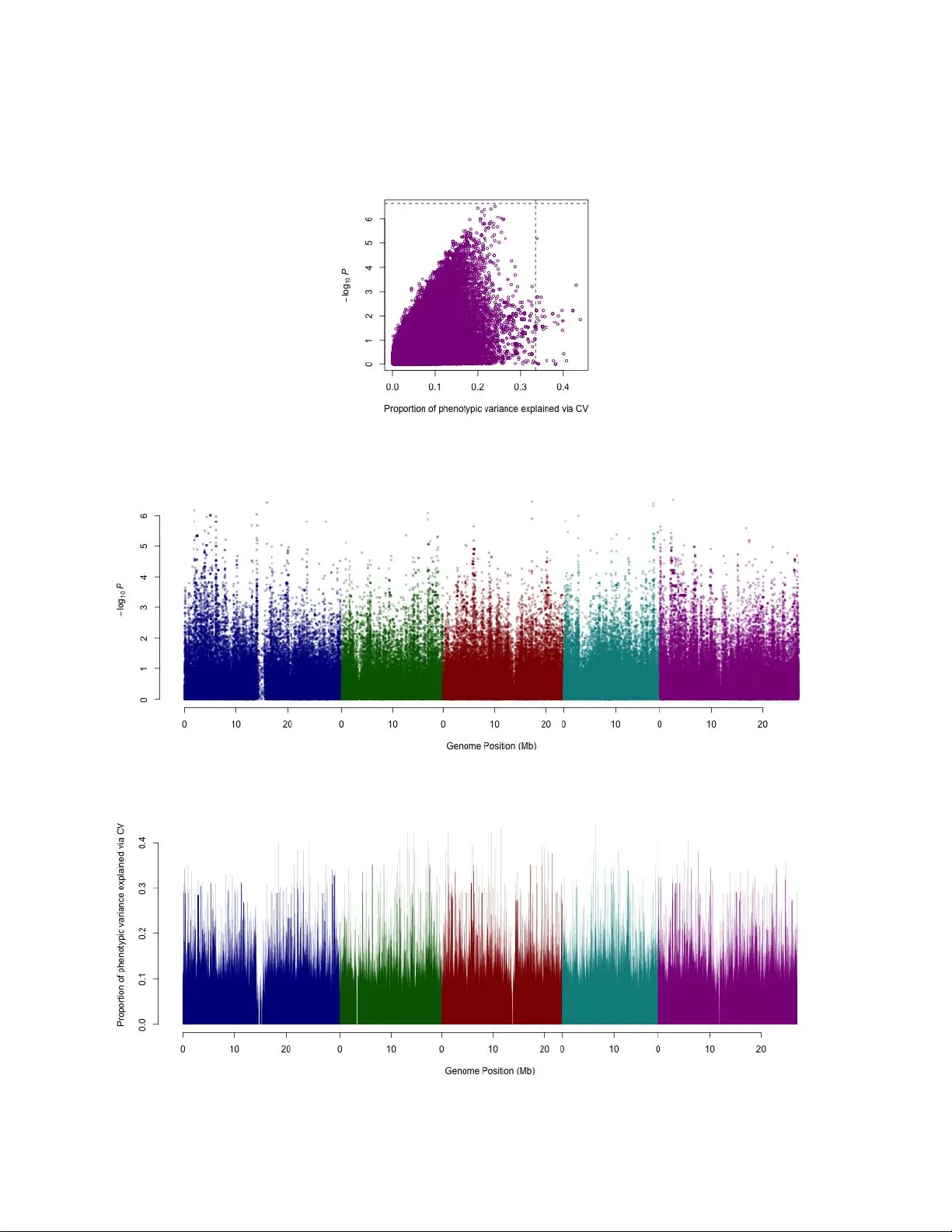
Revealing the missing heritability via cr oss-validated genome- wide association studies Xia Shen Division of Computational Genetics, Department of Clinical Sciences, Swedish University of Agricultural Sciences, Box 7078, SE-750 07 Uppsala, Sweden. Correspondence to: xia.shen@slu.se Presented her e is a simple method for cross-validated genome-wide association studies (cvGW AS). Focusing on phenotype prediction, the method is able to r eveal a significant amount of missing heritability by properly selecting a small number of loci with implicit predictive ability . The r esults pr ovide new insights into the missing heritability problem and the underlying genetic architectur e of complex traits. Recently , the case of missing heritability has drawn a lot of attention in genetics of complex traits 1,2,3,4,5,6,7 . It has been widely noticed that for many complex traits, the loci uncovered by means of e.g. genome-wide association studies (GW AS) could only explain a minor proportion of the phenotypic variance, even though the observed heritability of the trait is much higher . Strategies have been proposed to search for the sources of such missing heritability 4 , e.g. capturing additive genetic variance using polygenic ef fects across the genome 5,8 and mapping quantitative trait loci (QTL) using a powerful design 7 . However , even the use of all the genomic variants could not fully explain the missing heritability . Here, I propose a simple method to perform association mapping based on genomic variants’ predictive ability , explain the reason why the estimation of narrow sense heritability using all the markers across the genome is not reliable, and show that the underlying 1 1 2 3 4 5 6 7 8 9 10 11 12 13 14 15 16 17 18 19 20 21 22 23 24 heritability can be much higher than the conventional estimate and can even be well captured by a rather small number of QTL. Forty-nine traits in Arabidopsis thaliana 9 (9 flowering, 21 developmental, 12 defense and 7 ionomics) were analyzed, with the sample size varied from 84 to 194 inbred lines. The Arabidopsis accessions were genotyped using a 250K SNP (single nucleotide polymorphism) array , where 216,130 SNPs were available in the analysis. Instead of screening the genome using ordinary GW AS p -values, each SNP was assessed for their individual predictive ability by a 5-fold cross validation, i.e. the samples were split into a training (80%) and a test (20%) set for five replicates, without overlap among the five test sets. A linear regression of the phenotype on the SNP genotype was fitted in the training set for each marker , and the estimated model was used to perform out-of- sample prediction in the test set. The predictive ability of an individual SNP was evaluated via an R 2 , which is the squared correlation coeffic ient between the true phenotypic measurements and their predicted values in each of the five test sets. The mean of the five R 2 values, denoted as R 2 SNP , provided an estimate of the proportion of phenotypic variance captured by the SNP . It should be noted that such a predictive ability measurement is not a function of the p -value in ordinary GW AS ( e.g. Fig. 1 ). Namely , the p -values obtained in GW AS tend to under-estimate the predictive performance of the SNPs. Comparison of the association results based on p -values and R 2 SNP for all the analyzed traits are given in Supplementary Figure 1-49 . For each trait, among the top 0.05% of the SNPs ( n = 108) that had the highest R 2 SNP , the best subset with no more than 5 SNPs was selected by a forward stepwise selection procedure, based on a cross-validated assessment of their joint predictive power 10 . In order to compare the narrow sense heritability explained by the selected subset of SNPs ( h 2 QTL ) with that explained by the entire genome ( h 2 G ), another 5-fold cross validation was conducted. Both a random ef fects model using 2 25 26 27 28 29 30 31 32 33 34 35 36 37 38 39 40 41 42 43 44 45 46 47 48 49 only the selected SNPs (the QTL) as explanatory variables and a whole-genome ridge regression (SNP-BLUP 1 1,12 ) were fitted in the training sets and used for predicting the phenotypic values in the test sets. h 2 QTL and h 2 G were estimated as the mean of the corresponding five squared correlation coefficients between the true a nd the predicted values 5 . For most traits, as shown in Figure 2 , the small number of QTL had substantial advantage over the whole genome in terms of captured narrow sense heritability . The results indicated similar genetic architecture for the traits that belong to the same type. For instance, the defense and ionomics traits showed rather sparse architecture, whereas the flowering traits tended to be more polygenic. Interestingly , two gene expression traits of FRI and FLC , although regarded as flowering-related, appeared to have sparse architectures. For all the analyzed traits, details about the selected QTL and the heritability estimates are provided in Supplementary T able 2 . As a proof of concept, the results clearly showed that assessing the total narrow sense heritability using a large number of markers across the genome 5,7,8 is not a valid approach. The main re ason is that one has to substantially sacrifice the precision of the estimated QTL ef fects when incorporating too many markers as explanatory variables. When the QTL effects or the ef fects of the SNPs tagging the causal loci are properly estimated, the heritability inherited by the causal loci can be much better revealed than the entire genome. The results indicated that most of the missing heritability was missed by improper analytical methods. Beyond statistical significance in GW AS, more functional loci of complex traits can actually be revealed via assessments based on predictive performance. 3 50 51 52 53 54 55 56 57 58 59 60 61 62 63 64 65 66 67 68 69 70 Methods Software & URLs . The Arabidopsis thaliana GW AS data set is available at: https:// cynin.gmi.oeaw .ac.at/home/resources/atpolydb . All the analysis was conducte d in R 13 : http:// www .R-project.org /. The association mapping based on cross-validated R 2 SNP has been implemented in the “cvGW AS” package: https://r -forge.r -project.or g/projects/cvgwas/ . The forward stepwise selection procedure was executed by the “FWDselect” package 14 : http://cran.r -project.org/ web/packages/FWDselect/ . The random QTL effects model was fitted by the “hglm” package 15 : http://cran.r -project.org/web/packages/hglm/ . The whole-genome ridge regression (SNP-BLUP) was fitted by the “bigRR” package 12 : http://cran.r -project.org/web/packages/bigRR/ . 4 71 72 73 74 75 76 77 78 79 Figure Legends Figure 1: Comparison of the SNPs pr edictive ability and p -values for FRI gene expression . The predictive ability is assessed by R 2 SNP (“Proportion of phenotypic variance explained via CV”), where CV stands for “cross validation”. The p -values were obtained using W ilcoxon test. The horizontal line indicates the Bonferroni-corrected genome-wide significant threshold, and the vertical line shows the cut-off that de termines which SNPs are to be passed onto the forward selection procedure. Figure 2: Comparison of the narr ow sense heritability captur ed by the selected QTL ( h 2 QTL ) and the whole genome ( h 2 G ) . Each colored point represents an analyzed trait. The color of each point shows the type of the trait, where blue, red, green and pink refer to flowering, developmental, defense and ionomics traits, respectively . The size of each point is proportional to the number of QTL selected (from 2 to 5). The cross on each point shows the standard error estimates based on the cross validation. The dashed line indica tes equality of h 2 QTL and h 2 QTL as a visual guide. Supplementary T able 1-2 and Supplementary Figure 1-49 are available as Supplementary Information from the journal website. 5 References 1. Maher , B. Natur e 456 , 18-21 (2008) 2. Manolio, T . A. et al. Natur e 461 , 747-753 (2009) 3. Slatkin, M. Genetics 182 , 845-850 (2009) 4. Eichler , E. E. et al. Nat. Rev . Genet . 11 , 446-450 (2010) 5. Makowsky , R. et al. PL o S Genet . 7 , e1002051 (201 1) 6. Zuk, O., Hechter , E., Sunyaev , S. R. & Lander, E. S. Pr oc. Natl. Acad. Sci. USA 109 , 1 193-1 198 (2012) 7. Bloom, J. S. et al. Natur e 494 , 234-237 (2013) 8. Y ang, J. et al. Nat. Genet. 42 , 565-569 (2010). 9. Atwell, S. et al. Natur e 465 , 627-631 (2010). 10. Miller , A. Chapman & Hall (2002). 11. Meuwissen, T . H. E., Hayes, B. J. and Goddard, M. E. Genetics 157 , 1819-1829 (2001). 12. Shen, X., Alam, M., Fikse, F . and Rönnegård, L. Genetics 193 , 1255-1268 (2013). 13. R Core T eam. R Foundation for Statistical Computing, V ienna, Austria (2013). 14. Sestelo, M., V illanueva, N. M. and Roca-Pardinas, J. Discussion Papers in Statistics and Operation Resear ch , 13/02 (2013). 15. Rönnegård, L., Shen, X. and Alam, M. The R Journal 2 (2), 20-28 (2010). 6 Acknowledgement X.S. is funded by a Future Research Leaders grant from Swedish Foundation for Strategic Research (SSF) to Örjan Carlborg. 7 0.0 0.2 0.4 0.6 0.8 0.0 0.2 0.4 0.6 0.8 Propor tion of phenotypic v ariance explained by the whole genome (SNP − BLUP) Propor tion of phenotypic v ariance explained by the QTL Figure 1 Figure 2 This document contains the Supplementary Information for Revealing the missing heritability via cross-validated genome-wide association studies by Shen, X. (2013) Remarks: • The Excel table format of Supplementary T able 2 can be downloaded at: https:// docs.google.com/file/d/0B2ixEvB0Gwt6SWhZcW1KQmx2Wmc/edit?usp=sharing • In Supplementary Figure 1-49 , the horizontal dashed line in e ach top panel is the Bonferroni- corrected genome-wide significance threshold, and the vertical is the cut-of f for selecting candidate SNPs to be passed onto the forward selection procedure. The phenotypic variance explained in the bottom panels was estimated by R 2 SNP . • The link provided in Methods for the package “cvGW AS” is the project home page. For package download: https://r -forge.r -project.org/R/?group_id=1694 . If the package is being built on R- Forge, refer to https://r -forge.r -project.org/scm/viewvc.php/pkg/R/cvscore.R? view=markup&revision=2&root=cvgwas for the source code of the main function cvscore(), which is a directly usable add-on function for the GW A analysis package GenABEL (Aulchenko 2007 Bioinformatics). Supplementary T able 1: Phenotypes analyzed. Refer to Atwell et al . (2010) for further details about phenotype description and scoring. Phenotype ID Ty p e Sample size Description Growth Conditions SD 3 Flowering 162 Days to flowering time (FT) under Long Day (LD) and Short Day(SD) +/- vernalization. 18 ℃ , 8 hrs daylight. FT10 5 Flowering 194 Flowering time (FT) 10 ℃ , 16 hrs daylight. FT16 6 Flowering 193 Flowering time (FT) 16 ℃ , 16 hrs daylight. FT22 7 Flowering 193 Flowering time (FT) 22 ℃ , 16 hrs daylight. Emco5 9 Defense 86 Disease presence or absence following inoculation with each isolate. 20-22 ℃ , 10 hrs daylight, 70% humidity . Emwa1 10 Defense 85 Disease presence or absence following inoculation with each isolate. 20-22 ℃ , 10 hrs daylight, 70% humidity . Hiks1 12 Defense 84 Disease presence or absence following inoculation with each isolate. 20-22 ℃ , 10 hrs daylight, 70% humidity . Lithium (Li7) 14 Ionomics 93 In planta ion concentration. 20 ℃ , 16 hrs daylight. Sulfur (S34) 19 Ionomics 93 In planta ion concentration. 20 ℃ , 16 hrs daylight. Potassium (K39) 20 Ionomics 93 In planta ion concentration. 20 ℃ , 16 hrs daylight. Manganese (Mn55) 22 Ionomics 93 In planta ion concentration. 20 ℃ , 16 hrs daylight. Iron (Fe56) 23 Ionomics 93 In planta ion concentration. 20 ℃ , 16 hrs daylight. Cobalt (Co59) 24 Ionomics 93 In planta ion concentration. 20 ℃ , 16 hrs daylight. Zinc (Zn66) 27 Ionomics 93 In planta ion concentration. 20 ℃ , 16 hrs daylight. AvrRpm1 33 Defense 84 Hypersensitive response. 20 ℃ , 12 hrs daylight. FLC 43 Flowering 167 FLC and FRI gene expression. Growth in greenhouse, ~20-22 ℃ , 16 hrs daylight. FRI 44 Flowering 164 FLC and FRI gene expression. Growth in greenhouse, ~20-22 ℃ , 16 hrs daylight. 8W GH LN 46 Flowering 163 LN at FT . 20-22 ℃ , natural light from the middle of October 2002 till March 2003, vernalized (8 wks, 4 ℃ , 8 hrs daylight). 0W GH LN 48 Flowering 135 LN at FT . 20-22 ℃ , natural light from the middle of October 2002 till March 2003. FT Diameter Field 58 Flowering 180 Plant diameter at flowering (field). Growth in field or greenhouse (20 ℃ , 16 hrs daylight), started in October . Phenotype ID Ty p e Sample size Description Growth Conditions At1 65 175 At1 CFU2 66 175 As CFU2 68 175 Bs 69 175 Bs CFU2 70 175 At2 71 175 At2 CFU2 72 175 As2 73 175 DW 76 Developmental 95 Dry weight of plants. Plants were grown for 7 weeks at 23 ℃ . Silique 22 159 Developmental 95 Silique length. 22 ℃ , 16 hrs daylight. Germ 10 161 Developmental 177 Days to germination. Stratified for 3 days at 4 ℃ in the dark, followed by growth at 10 ℃ with 16 hrs daylight. Germ 16 162 Developmental 176 Days to germination. Stratified for 3 days at 4 ℃ in the dark, followed by growth at 16 ℃ with 16 hrs daylight. Width 10 164 Developmental 176 Plant diameter . 10 ℃ , 16 hrs daylight. Width 16 165 Developmental 175 Plant diameter . 16 ℃ , 16 hrs daylight. Width 22 166 Developmental 175 Plant diameter . 22 ℃ , 16 hrs daylight. Chlorosis 16 168 Developmental 176 Visual chlorosis presence. 16 ℃ , 16 hrs daylight. Anthocyanin 10 170 Developmental 177 Visual anthocyanin presence. 10 ℃ , 16 hrs daylight. Anthocyanin 16 171 Developmental 176 V isual anthocyanin presence. 16 ℃ , 16 hrs daylight. Anthocyanin 22 172 Developmental 177 V isual anthocyanin presence. 22 ℃ , 16 hrs daylight. Leaf serr 10 173 Developmental 174 Level of leaf serration. 10 ℃ , 16 hrs daylight. Leaf roll 16 177 Developmental 176 Level of roll presence. 16 ℃ , 16 hrs daylight. Rosette Erect 22 179 Developmental 176 Presence of rosette erectness. 22 ℃ , 16 hrs daylight. Seedling Growth 272 Developmental 101 Seedling growth rate. Seeds were grown for one week in the greenhouse under long day (16 hours light). Phenotype ID Ty p e Sample size Description Growth Conditions V ern Growth 273 Developmental 111 V egetative growth rate during vernalization. Seeds were grown for one week in the greenhouse under long day (16 hours light), vernalized for 4 weeks (4 ℃ , 16h light, 50% relative humidity). After V ern Growth 274 Developmental 111 V egetative growth rate after vernalization. Seeds were grown for one week in the greenhouse under long day (16 hours light), vernalized for 4 weeks (4 ℃ , 16 hrs light, 50% relative humidity)and then returned to greenhouse. Secondary Dormancy 277 Developmental 94 Decrease in germination rate after prolonged exposure to cold temperature. Fully after-ripened seeds were treated with a 1 and 6-week long exposure to 4 ℃ . Germ in dark 278 Developmental 94 Germination in the dark. 4 ℃ , in the dark. DSDS50 279 Developmental 11 0 Duration of seed dry storage required for 50% of the seeds to germinate. Dry storage, followed by 25 ℃ , 12 hrs day , 20 ℃ , 12 hrs night for 1 week. Storage 56 days 283 Developmental 111 Primary dormancy . 56 days dry storage. Supplementary,Table,2 Summary,of,selected,QTL,for,each,analyzed,trait,and,the,heritability,estimates,compared,to,those,by,the,whole,genome. !" #$%%&'()*+)*,!*%-.$/-0-.1,*).-2$.*3,$),.!*,2*$+,&4,.!*,)56$%*3,7&%%*0$.-&+,7&*44-7-*+.),/*.'**+,.!*,.%6*,$+3,.!*,8%*3-7.*3,8!*+&.18*,-+,$,9(4&03,7%&)),:$0-3$.-&+; <&%,!"=>?@A,$,%$+3&2,*44*7.),2&3*0,6)-+B,&+01,.!*,>?@,$),*C80$+$.&%1,:$%-$/0*),'*%*,4-..*3;,<&%,!"=DE#FGEA,$,'!&0*(B*+&2*,%-3B*,%*B%*))-&+,6)-+B,$00,.!*,H#I),'*%*,4-..*3; )* H.$+3$%3,*%%&%,*).-2$.*3,:-$,$,9(4&03,7%&)),:$0-3$.-&+; CHROMOSOME POSITION HJ <0&'*%-+B K L9MN"OM P;QPQN P;PQMP P;Q9KR P;PN99 K KOMPNPMP N KOM"NM"" N KOM"MPNP L KQPOLMKM
Original Paper
Loading high-quality paper...
Comments & Academic Discussion
Loading comments...
Leave a Comment