On GROUSE and Incremental SVD

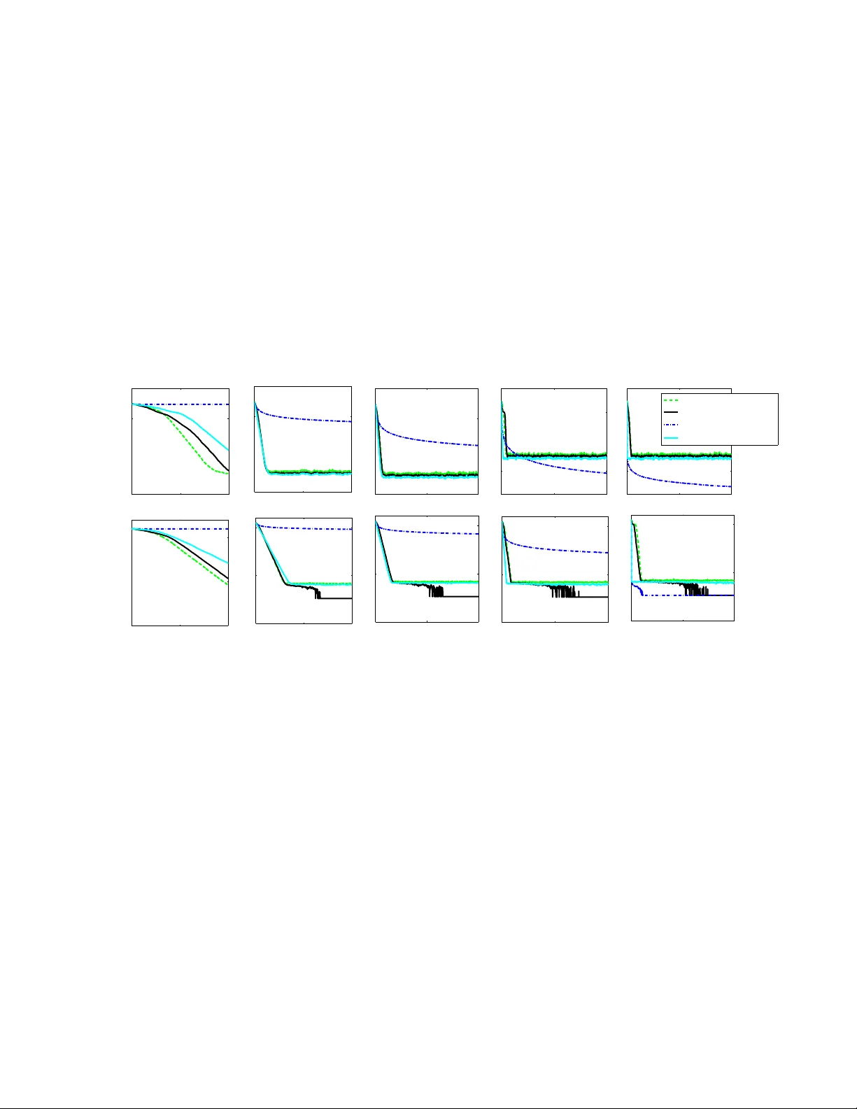
On GR OUSE and Incremental SVD Laura Balzano Univ ersity of Michigan girasole@umich.edu Stephen J. Wright Univ ersity of W isconsin, Madison swright@cs.wisc.edu Abstract —GROUSE (Grassmannian Rank-One Update Sub- space Estimation) [1] is an incremental algorithm f or identifying a subspace of R n from a sequence of vectors in this subspace, where only a subset of components of each vector is re vealed at each iteration. Recent analysis [2] has shown that GR OUSE con verges locally at an expected linear rate, under certain assumptions. GROUSE has a similar flavor to the incremental singular value decomposition algorithm [4], which updates the SVD of a matrix follo wing addition of a single column. In this paper , we modify the incr emental SVD appr oach to handle missing data, and demonstrate that this modified approach is equivalent to GROUSE, for a certain choice of an algorithmic parameter . I . I N T RO D U C T I O N Subspace estimation and singular value decomposition have been important tools in linear algebra and data analysis for sev eral decades. They are used to understand the principal components of a signal, to reject noise, and to identify best approximations. The GROUSE (Grassmannian Rank-One Update Subspace Estimation) algorithm, described in [1], aims to identify a subspace of low dimension, given data consisting of a se- quence of vectors in the subspace that are missing many of their components. Missing data is common in such big-data applications as low-cost sensor networks (in which data often get lost from corruption or bad communication links), recom- mender systems (where we are missing consumers’ opinions on products they hav e yet to try), and health care (where a patient’ s health status is only sparsely sampled in time). GR OUSE was developed originally in an online setting, to be used with streaming data or when the principal components of the signal may be time-v arying. Se veral subspace estimation algorithms in the past [6] hav e also been dev eloped for the online case and ha ve ev en used stochastic gradient, though GR OUSE and the approach described in [3] are the first to deal with missing data. Recent dev elopments in the closely related field of matrix completion have shown that low-rank matrices can be recon- structed from limited information, using tractable optimization formulations [5], [7]. Gi ven this experience, it is not surprising that subspace identification is possible ev en when the re vealed data is incomplete, under appropriate incoherence assumptions and using appropriate algorithms. GR OUSE maintains an n × d matrix with orthonormal columns that is updated by a rank-one matrix at each iter - ation. The update strategy is redolent of other optimization appoaches such as gradient projection, stochastic gradient, and quasi-Newton methods. It is related also to the incremental singular value decomposition approach of [4], in which the SVD of a matrix is updated ine xpensiv ely after addition of a column. W e aim in this note to explore the relationship between the GR OUSE and incremental SVD approaches. W e show that when the incremental SVD approach is modified in a plausible way (to handle missing data, among other issues), we obtain an algorithm that is equiv alent to GROUSE. I I . G RO U S E The GR OUSE algorithm was developed for identifying an unknown subspace S of dimension d in R n from a sequence of vectors v t ∈ S in which only the components indicated by the set Ω t ⊂ { 1 , . . . , n } are re vealed. Specifically , when ¯ U is an (unknown) n × d matrix whose orthonormal columns span S , and s t ∈ R d is a weight vector , we observe the following subv ector at iteration t : ( v t ) Ω t = ( ¯ U s t ) Ω t (1) (W e use the subscript Ω t on a matrix or vector to indicate restriction to the rows indicated by Ω t .) GR OUSE is described as Algorithm 1. It generates a sequence of n × d matrices U t with orthonormal columns, updating with a rank-one matrix at each iteration in response to the ne wly re vealed data ( v t ) Ω t . Note that GR OUSE makes use of a steplength parameter η t . It was sho wn in [2] that GR OUSE e xhibits local con vergence of the range space of U t to the range space of ¯ U , at an expected linear rate, under certain assumptions including incoherence of the subspace S with the coordinate directions, the number of components in Ω t , and the choice of steplength parameter η t . I I I . I N C R E M E N T A L S I N G U L A R V A L U E D E C O M P O S I T I O N The incremental SVD algorithm of [4] computes the SVD of a matrix by adding one (fully observed) column at a time. The size of the matrices of left and right singular vectors U t and V t grows as columns are added, as does the diagonal matrix of singular v alues Σ t . The approach is shown in Algorithm 2. Note that when the new vector v t is already in the range space of U t , we hav e r t = 0 , and the basic approach can be modified to avoid adding an extra dimension to the U , V , and Σ factors in this situation. If all vectors v t lie in a subspace S of dimension d , the modified method will not need to grow U t beyond size n × d . Algorithm 1 GROUSE Giv en U 0 , an n × d orthonormal matrix, with 0 < d < n ; Set t := 1 ; repeat T ake Ω t and ( v t ) Ω t from (1); Define w t := arg min w k [ U t ] Ω t w − [ v t ] Ω t k 2 2 ; Define p t := U t w t ; [ r t ] Ω t := [ v t ] Ω t − [ p t ] Ω t ; [ r t ] Ω C t := 0 ; σ t := k r t k k p t k ; Choose η t > 0 and set U t +1 := U t + (cos( σ t η t ) − 1) p t k p t k w T t k w t k + sin( σ t η t ) r t k r t k w T t k w t k . (2) t := t + 1 ; until termination Algorithm 2 Incremental SVD [4] Start with null matrixes U 0 , V 0 , Σ 0 ; Set t := 0 ; repeat Giv en new column vector v t ; Define w t := arg min w k U t w − v t k 2 2 = U T t v t ; Define p t := U t w t ; r t := v t − p t ; (Set r 0 := v 0 when t = 0 ); Noting that  U t Σ t V T t v t  = h U t r t k r t k i  Σ t w t 0 k r t k   V t 0 0 1  T , compute the SVD of the update matrix:  Σ t w t 0 k r t k  = ˆ U ˆ Σ ˆ V T , (3) and set U t +1 := h U t r t k r t k i ˆ U , Σ t +1 := ˆ Σ , V t +1 :=  V t 0 0 1  ˆ V . t := t + 1 ; until termination I V . R E L A T I N G G R O U S E TO I N C R E M E N TA L S V D Algorithms 1 and 2 are motiv ated in different ways and therefore differ in significant respects. W e now describe a vari- ant — Algorithm 3 — that is suited to the setting addressed by GR OUSE, and show that it is in fact equiv alent to GR OUSE. Algorithm 3, includes the following modifications. • Since only the subvector ( v t ) Ω t is available, the missing components of v t (corresponding to indices in the com- plement Ω C t := { 1 , 2 , . . . , n } \ Ω t ) must be “imputed” from the rev ealed components and from the current subspace estimate U t . • The singular value matrix Σ t is not carried o ver from one iteration to the next. In ef fect, the singular value estimates are all reset to 1 at each iteration. • W e allow an arbitrary rotation operator W t to be applied to the columns of U t at each iteration. This does not af fect the range space of U t , which is the current estimate of the underlying subspace S . • The matrix U t is not permitted to gro w beyond d columns. Algorithm 3 iSVD for Partially Observed V ectors Giv en U 0 , an n × d orthonormal matrix, with 0 < d < n ; Set t := 1 ; repeat T ake Ω t and ( v t ) Ω t from (1); Define w t := arg min w k ( U t ) Ω t w − ( v t ) Ω t k 2 2 ; Define [ ˜ v t ] i :=  [ v t ] i i ∈ Ω t [ U t w t ] i i ∈ Ω C t ; p t := U t w t ; r t := ˜ v t − p t ; Noting that  U t ˜ v t  = h U t r t k r t k i  I w t 0 k r t k  , we compute the SVD of the update matrix:  I w t 0 k r t k  = ˜ U t ˜ Σ t ˜ V T t , (4) and define ˆ U t to be the ( d + 1) × d matrix obtained by removing the last column from ˜ U t . Set U t +1 := h U t r t k r t k i ˆ U W t , where W t is an arbitrary d × d orthogonal matrix. t := t + 1 ; until termination Algorithm 3 is quite similar to an algorithm proposed in [3] (see Algorithm 4) but differs in its handling of the singular values. In [3], the singular v alues are carried over from one iteration to the next, but previous estimates are “do wn- weighted” to place more importance on the vectors ( v t ) Ω t from recent iterations. This feature is useful in a scenario in which the underlying subspace S is changing in time. GR OUSE also is influenced more by more recent vectors than older ones, thus has a similar (though less explicit) do wn- weighting feature. W e show no w that for a particular choice of η t in Algo- rithm 3, the Algorithms 1 and 3 are equiv alent. Any difference in the updated estimate U t +1 is eliminated when we define the column rotation matrix W t appropriately . Theor em 1: Suppose that at iteration t of Algorithms 1 and 3, the iterates U t are the same, and the new observ ations v t and Ω t are the same. Assume too that w t 6 = 0 and r t 6 = 0 . Define the following (related) scalar quantities: λ := 1 2 ( k w t k 2 + k r t k 2 + 1)+ 1 2 p ( k w t k 2 + k r t k 2 + 1) 2 − 4 k r t k 2 ; (5a) β := k r t k 2 + k w t k 2 k r t k 2 + k w t k 2 + ( λ − k r t k 2 ) 2 (5b) α := k r t k ( λ − k r t k 2 ) k r t k 2 + k w t k 2 + ( λ − k r t k 2 ) 2 (5c) η t := 1 σ t arcsin β = 1 σ t arccos( α k w t k ) , (5d) and define the d × d orthogonal matrix W t by W t :=  w t k w t k | Z t  , (6) where Z t is a d × d − 1 orthonormal matrix whose columns span the orthogonal complement of w t . For these choices of η t and W t , the iterates U t +1 generated by Algorithms 1 and 3 are identical. Pr oof: W e drop the subscript t freely throughout the proof. W e first derive the structure of the matrix ˆ U t in Algorithm 3, which is key to the update formula in this algorithm. W e hav e from (4) that  I w 0 k r k   I 0 w T k r k  =  I + w w T k r k w k r k w T k r k 2  = ˜ U ˜ Σ 2 ˜ U T , (7) and thus the columns of ˜ U are eigen vectors of this product matrix. W e see that the columns of the d × ( d − 1) orthonormal matrix Z t defined in (6) can be used to construct a set of eigen vectors that correspond to the eigenv alue 1 , since  I + w w T k r k w k r k w T k r k 2   Z t 0  =  Z t 0  . (8) T wo eigen vectors and eigenv alues remain to be determined. Using λ to generally denote one of these two eigen values and ( y T : β ) T to denote the corresponding eigen vector , we have  I + w w T k r k w k r k w T k r k 2   y β  = λ  y β  . (9) The first block row of this expression yields y + w ( w T y + k r k β ) = λy , which implies that y has the form αw for some α ∈ R . By substituting this form into the two block rows from (9), we obtain α (1 − λ ) w + w ( α k w k 2 + k r k β ) = 0 ⇒ α (1 + k w k 2 − λ ) + k r k β = 0 , (10) and α k r kk w k 2 + ( k r k 2 − λ ) β = 0 . (11) W e require also that the vector  y β  =  αw β  has unit norm, yielding the additional condition α 2 k w k 2 + β 2 = 1 . (12) (This condition verifies the equality between the “ arcsin ” and “ arccos ” definitions in (5d).) T o find the two possible values for λ , we seek non-unit roots of the characteristic polynomial for (7) and make use of the Schur form det  A B C D  = (det D ) det( A − B D − 1 C ) , to obtain det  I + w w T − λI k r k w k r k w T k r k 2 − λ  = ( k r k 2 − λ ) det  (1 − λ ) I + w w T − k r k 2 k r k 2 − λ w w T  = ( k r k 2 − λ ) det  (1 − λ ) I − λ k r k 2 − λ w w T  = (1 − λ ) d ( k r k 2 − λ )  1 − λ k w k 2 ( k r k 2 − λ )(1 − λ )  = (1 − λ ) d − 1  ( k r k 2 − λ )(1 − λ ) − λ k w k 2  = (1 − λ ) d − 1 ( λ 2 − λ ( k w k 2 + k r k 2 + 1) + k r k 2 ) , where we used det( I + aa T ) = 1 + k a k 2 . Thus the two non- unit eigen values are the roots of the quadratic λ 2 − λ ( k w k 2 + k r k 2 + 1) + k r k 2 . (13) When r 6 = 0 and w 6 = 0 , this quadratic takes on positive values at λ = 0 and when λ ↑ ∞ , while the value at λ = 1 is negati ve. Hence there are two roots, one in the interval (0 , 1) and one in (1 , ∞ ) . W e fix λ to the larger root, which is given explicitly by (5a). The corresponding eigenv alue is the first column in the matrix ˜ U t , and thus also in the matrix ˆ U t . It can be shown, by reference to formulas (5a) and (13), that the values of β and α defined by (5b) and (5c), respecti vely , satisfy the conditions (10), (11), (12). W e can no w assemble the leading d eigenv ectors of the matrix in (7) to form the matrix ˆ U as follows: ˆ U :=  αw Z t β 0  . Thus, with W t defined as in (6), we obtain ˆ U W T t =  αw Z t β 0  " w T k w k Z T t # = " α k w k w w T + Z t Z T t β k w k w T # . Therefore, we hav e from the update formula for Algorithm 3 that U t +1 = h U t r k r k i ˆ U W T t = U t  α k w k w w T + Z t Z T t  + β r k r k w T k w k . By orthogonality of W t , we hav e I = W W T = w w T k w k 2 + Z t Z T t ⇒ Z t Z T t − I − w w T k w k 2 . Hence, by substituting in the expression above, we obtain U t +1 = U t  α w w T k w k +  I − w w T k w k 2  + β r k r k w T k w k = U t +  ( α k w k − 1) w k w k + β r k r k  w T k w k , which is identical to the update formula in Algorithm 1 provided that cos σ t η t = α k w t k , sin σ t η t = β . These relationships hold because of the definition (5d) and the normality relationship (12). Algorithm 4 Another iSVD approach for Partial Data [3] Giv en U 0 , an arbitrary n × d orthonormal matrix, with 0 < d < n ; Σ 0 , a d × d diagonal matrix of zeros which will later hold the singular values. Set t := 1 ; repeat Compute w t , p t , r t as in Algorithm 3. Compute the SVD of the update matrix:  β Σ t w t 0 k r t k  = ˆ U ˆ Σ ˆ V T , for some scalar β ≤ 1 and set U t +1 := h U t r t k r t k i ˆ U , Σ t +1 := ˆ Σ . t := t + 1 ; until termination V . S I M U L A T I O N S T o compare the algorithms presented in this note, we ran simulations as follows. W e set n = 200 and d = 10 , and defined ¯ U (whose columns span the target subspce S ) to be a random matrix with orthonormal columns. The vectors v t were generated as ¯ U s t , where the components of s t are N (0 , 1) i.i.d. W e also computed a different n × d matrix with orthonormal columns, and used that to initialize all algorithms. W e compared the GR OUSE algorithm (Algorithm 1) with our proposed missing data iSVD (Algorithm 3). Although, as we show in this note, these algorithms are equiv alent for a particular choice of η t , we used the different choice of this parameter prescribed in [2]. Finally , we compared to the incomplete data iSVD proposed in [3], which is summarized in Algorithm 4. This approach requires a parameter β which down-weights old singular value estimates. W e obtained the performance for β = 0 . 95 ; performance of this approach degraded for values of β less than 0 . 9 . The error metric on the y-axis is d − k U T t ¯ U k 2 F ; see [2] for details of this quantity . V I . C O N C L U S I O N W e have shown an equiv alence between GROUSE and a modified incemental SVD approach. The equiv alence is of interest because the two methods are moti v ated and con- structed from different perspecti ves — GR OUSE from an optimization perspectiv e, and incremental SVD from linear algebra perspectiv e. R E F E R E N C E S [1] Laura Balzano, Robert Nowak, and Benjamin Recht. Online identification and tracking of subspaces from highly incomplete information. In Pr oceedings of the Allerton confer ence on Communication, Contr ol, and Computing , 2010. [2] Laura Balzano and Stephen J. Wright. Local conv ergence of an algorithm for subspace identification from partial data. Submitted for publication. Preprint a vailable at http://arxiv .org/abs/1306.3391. [3] M. Brand. Incremental singular value decomposition of uncertain data with missing values. Eur opean Conference on Computer V ision (ECCV) , pages 707–720, 2002. [4] James R. Bunch and Christopher P . Nielsen. Updating the singu- lar value decomposition. Numerische Mathematik , 31:111–129, 1978. 10.1007/BF01397471. [5] Emmanuel Cand ` es and Benjamin Recht. Exact matrix completion via con vex optimization. F oundations of Computational Mathematics , 9(6):717–772, 2009. [6] Pierre Comon and Gene Golub. Tracking a few extreme singular values and vectors in signal processing. Proceedings of the IEEE , 78(8), August 1990. [7] Benjamin Recht. A simpler approach to matrix completion. J ournal of Machine Learning Researc h , 12:3413–3430, 2011. 0 2000 4000 10 − 5 10 0 10% entries observed angle btw est and true subspace 0 2000 4000 10 − 5 10 0 30% entries observed noise var = 0.001 0 2000 4000 10 − 5 10 0 50% entries observed 0 2000 4000 10 − 5 10 0 95% entries observed 0 2000 4000 10 − 5 10 0 100% entries observed Alg 1 with step as in [2] Alg 3 Alg 4  =1 [3] Alg 4  =.95 [3] 0 2000 4000 10 − 10 10 − 5 10 0 noise var = 1e − 07 0 2000 4000 10 − 20 10 − 10 10 0 0 2000 4000 10 − 20 10 − 10 10 0 # vectors observed 0 2000 4000 10 − 20 10 − 10 10 0 0 2000 4000 10 − 20 10 − 10 10 0 Fig. 1. Results for the algorithms described in this paper . Algorithm 4 with β = 1 and full data is equivalent to the original incermental SVD (Algorithm 2). This algorithm performs the best when all entries are observed or when just a small amount of data is missing and noise is present. Algorithm 4 with β = 0 . 95 and full data at first conver ges quickly as with β = 1 but flatlines much earlier . GROUSE (Algorithm 1) with the step as prescribed in [2] does the best when a very small fraction of entries are observed, approaching the theoretical minimum (see [2] for details). With low noise and missing data, our iSVD method (Algorithm 3) av erages out the noise, given enough iterations. Otherwise the algorithms perform equivalently .