Temporal and Spatial Independent Component Analysis for fMRI data sets embedded in a R package

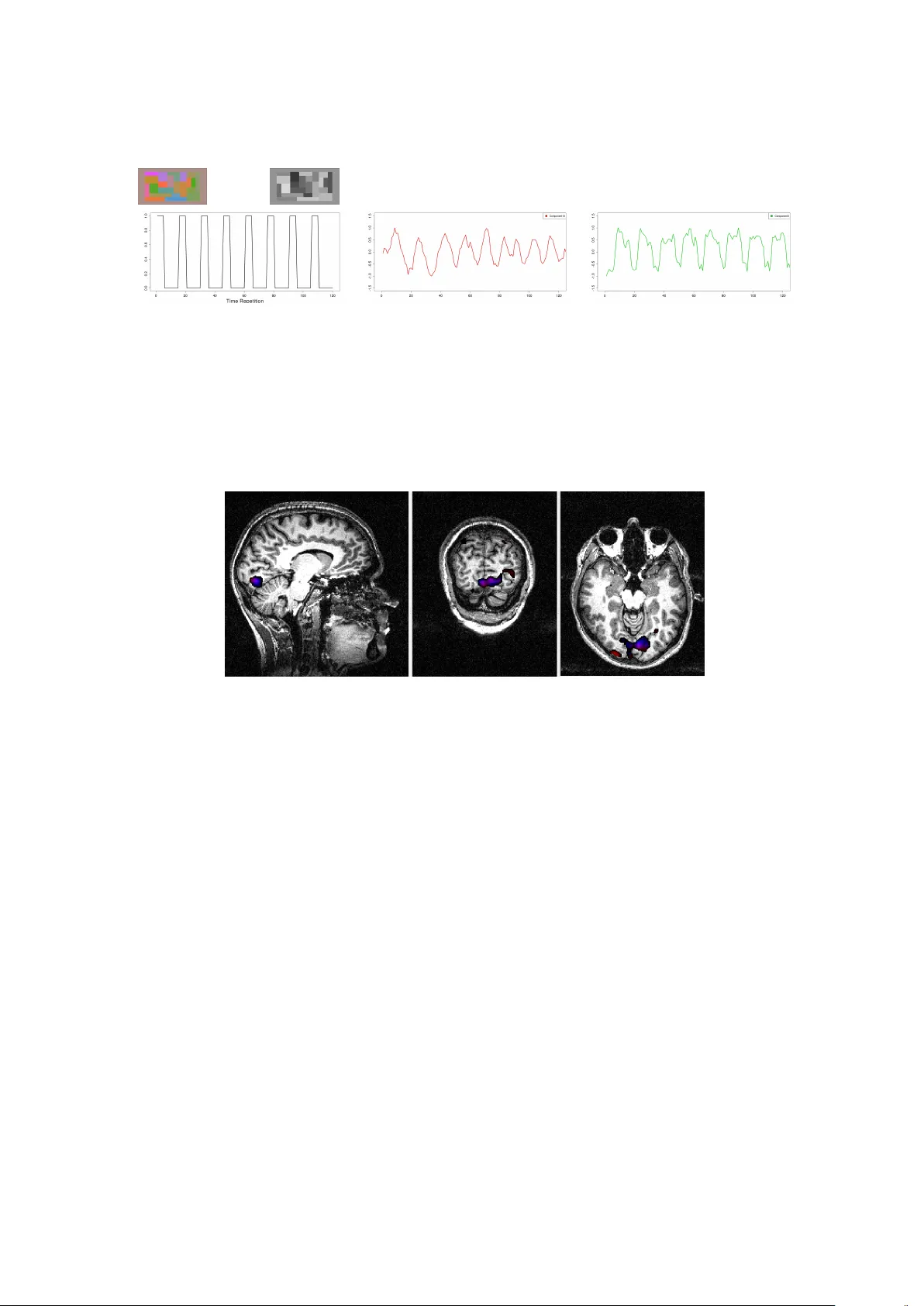
T emp oral and Spatial Indep enden t Comp onen t Analysis for fMRI data sets em b edded in a R pac k age C ´ ecile Bordier GIN Mic hel Do jat GIN Pierre Lafa y e de Mic heaux Univ ersit´ e de Mon tr´ eal Abstract F or statistical analysis of functional Magnetic Resonance Imaging (fMRI) data sets, w e propose a data-drive n approach based on Independent Component Analysis (ICA) im- plemen ted in a new ver sion of the AnalyzeFMRI R pack age. F or fMRI data sets, spatial dimension b eing muc h greater than temporal dimension, spatial ICA is the tractable ap- proac h generally prop osed. How ever, for some neurosc ien tific applications, temp oral inde- p endence of source signals can b e assumed and temp oral ICA b ecomes then an attracting exploratory technique. In this work, we use a classical linear algebra result ensuring the tractabilit y of temporal ICA. W e rep ort several exp eriments on syn thetic data and real MRI data sets that demonstrate the p otential interest of our R pack age. Keywor ds : Multiv ariate analysis, T emp oral ICA, Spatial ICA, Magnetic Resonance Imaging, Neuroimaging. 1. In tro duction Magnetic Resonance Imaging (MRI) is no w a prominen t non-inv asive neuroimaging tec hnique largely used in clinical routine and adv anced brain research. Its success is largely due to a com bination of at least three factors: 1) sensitivity of MR signal to v arious physiological pa- rameters that c haracterize normal or pathological living tissues (such as diffusion properties of H 2 0 molecules, relaxation time of proton magnetization or blo o d oxygenation) leading to a v ast panoply of MRI mo dalities (resp ectiv ely restricted in our example to diffusion MR imag- ing, w eighted structural images and functional MRI); 2) constant hardware improv emen ts (e.g. mastering high field homogeneous magnets and high linear magnetic field gradients re- sp ectiv ely allo ws an increasing of spatial resolution or a reduction of acquisition time); and 3) sustained efforts in v arious lab oratories to dev elop robust softw are: for image pro cessing (to de-noise, segment, realign, fusion or visualize MR brain images), for computational anatomy leading to the exploration of brain structure mo difications during learning, brain dev elopmen t or pathology ev olution and for time course analysis of functional MRI data. Statisticians play a key role in this last factor since data pro duced are complex: noisy , highly v ariable b etw een sub jects, massive and, for functional data, highly correlated b oth spatially and temporally ( Lange ( 2003 )). F unctional MRI (fMRI) allows to detect the v ariations of cerebral blo o d ox ygen level induced b y the brain activit y of a sub ject, lying inside a MRI scanner, in resp onse to v arious sensory- 2 T emp oral and Spatial Indep endent Comp onent Analysis for fMRI data sets motor or cognitive tasks ( Chen and Ogaw a ( 1999 )). The fMRI signal is based on changes in magnetic susceptibilit y of the blo o d during brain activ ation. It is a non-in v asive and indi- rect detection of brain activity: the signal detected is filtered by the hemo dynamic resp onse function (HRF) and the neuro-v ascular coupling is only partially explained ( Logothetis and Pfeuffer ( 2004 )). The main goal of fMRI exp eriments is to explore, in a repro ducible w a y , the cortical netw orks implicated in pre-defined stim ulation tasks in a cohort of normal or pathological sub jects. The low signal to noise ratio obtained in functional images requires to rep eat the sequence of stimuli sev eral times ( Henson ( 2004 )) and to enroll a sufficient n umber of sub jects ( Thirion, Pinel, Meriaux, Ro che, Dehaene, and Pol ine ( 2007 )). In general, the data resulting from an fMRI exp erimen t consist in a set indexed with time (typically many h undred) of 3D dimensional functional images with a 3 × 3 × 3 mm 3 spatial resolution, and in a structural (or anatomical) image with a 1 × 1 × 1 mm 3 resolution used to accurately localize functional activ ations. Note that a 3D image is in fact an arra y of man y v oxels’s in tensities. V arious pre-pro cessing steps are required to correct functional i mages from possible head sub- ject mo vemen t, to realign functional and anatomical individual images and, for group studies, all individual data sets in a common referen tial. A spatial smo othing (e.g. using a gaussian k ernel) is generally applied to functional images to comp ensate for p otent ial mis-realignmen t and enhance the signal-to-noise ratio. Sev eral frameworks hav e b een prop osed to date for statistical analysis of these pre-pro cessed sets of functional data (see Lazard ( 2008 )’s b o ok for a recen t rev iew). The commonly used sta- tistical approach , massiv ely univ ariate, considers each vo xel indep endently from each other using regression techniques ( F riston, Holmes, P oline, F rith, and F rack o wiak ( 1995 )); Bull- more, Brammer, Williams, Rab e-Hesketh, Janot, David, Mellers, How ard, and Sham ( 1996 )). It is av ailable in freew are pac k ages such as FSL ( http://www.fmrib.ox.ac.uk/fsl/ ), SPM ( http://www.fil.ion.ucl. ac.uk/spm/ ), BrainVisa ( http://brainvisa.info/ ) or NIPY ( http://nipy.sourceforge .net/ ). The time series resp onse at each v oxel is mo deled as a stationary linear filter where the finite impulse resp onse corresp onds to a mo del of the HRF. This leads to the specification of a general linear model (noted GLM thereafter; not t o be con- founded with the Generalized Linear Mo del) where the design matrix contains, for eac h time p oin t, the o ccurrences of the successiv e stimuli (regressors) conv olv ed with the HRF mo del. Other regressors can b e seamlessly in tro duced to model possible confounds. Many refinemen ts to this approac h hav e b een prop osed ( Nic hols and Holmes ( 2002 ); F riston, Stephan, Lund, Morcom, and Kieb el ( 2005 ); Ro che, Meriaux, Keller, and Thirion ( 2007 )). Spatial smo oth- ness of the activ ated areas, normal distribution and indep endence of the error terms and a predefined form of the HRF used as a con volution kernel are the main a priori incorp orated in to the GLM. This mo del-driv en approach allows to test, using standard Studen t or Fisher tests, the activ ated regions against a desired h yp othesis by sp ecifying comp ositions of regres- sors. It is largely used essentially b ecause of its flexibility in mo del sp ecification allowing to test v arious h yp othesis represen ted in corresponding statistical parametric maps. Clearly , the v alidity of the interpretation of these maps dep ends on the accuracy of the sp ecified mo del. An alternative exploratory (data-driv en) approac h relies on multiv ariate analysis based on Indep enden t Component Analysis (ICA). ICA performs a blind separation of independent sources from a complex mixture of man y sources of signal and noise. In this approac h, relying on the int rinsic structure of the data, no assumptions ab out the form of the HRF or the p os- sible causes of resp onses are inserted. Only the num b er of sources or comp onents to search for could even tually b e sp ecified. T o identify a n umber of unknown sources of signal, ICA as- sumes that these sources are mu tually and statistically indep endent in space (sICA) or time C ´ ecile Bordier, Michel Do jat, Pierre Lafay e de Mic heaux 3 (tICA). This assumption is particularly relev ant to biological time-series ( F riston ( 1998 )). F or fMRI data set analyses, sICA is preferred b ecause temp oral p oint s (few hundr eds, corre- sp onding to each o ccurrence of a functional image acquisition) are small compared to spatial ones (more than 10 5 , corresp onding to the num b er of v oxels contained in a functional image) leading for tICA to a com putationnaly in tractable mixing matrix ( McKeo wn, Makeig, Bro wn, Jung, Jindermann, Bell, and Sejnowski ( 1998 )). Ho wev er, temp oral ICA could b e relev ant for some neuroscientific applications where temp oral independence of sources can b e assumed ( Calhoun, Adali, P earlson, and Pek ar ( 2001 )). In this context, these authors wrote “... Note that tICA is typic al ly much mor e c omputational ly demanding than sICA for functional MRI applic ations b e c ause of a higher sp atial than temp or al dimension and c an gr ow quickly b eyond pr actic al fe asibility. Thus a c ovarianc e matrix on the or der of N 2 (wher e N is the numb er of sp atial voxels of inter est) must b e c alculate d. A c ombination of incr e ase d har dwar e c ap acity as wel l as mor e advanc e d metho ds for c alculating and storing the c ovarianc e matrix may pr ovide a solution in the futur e ...” . In this pap er, we prop ose to use a classical linear algebra result to alleviate the aforementioned computational burden. The pap er is structured as follows. First, in Section 2 we briefly describ e the principle of temp oral and spati al ICA in the context of fMRI data set analysis and detail the mathe matical dev elopments we prop ose for ensuring temp oral ICA tractabilit y . In Section 3, w e describe the curren t v ersion of the AnalyzeFMRI R pack age (see Marc hini and Lafa ye de Micheaux ( 2010 )), whic h is the first R pack age designed for the pro cessing and analysis of large anatomical and functional MRI data sets. It was initiated b y J. Marc hini ( Marchini ( 2002 )), who passed the torch in 2007 to the third author of this pap er. This pack age includes, compared to its initial v ersion, our recen t extensions: i.e. NIFTI format managemen t, cross-platform visualization based on Tcl-Tk comp onents and temp oral (and spatial) ICA (TS-ICA). W e rep ort, in Section 4, results using synthetic data and real MRI data sets coming from h uman visual exp eriment s, obtained using TS-ICA. Finally , w e conclude ab out the interest of the AnalyzeFMRI pack age and our extensions for the exploration of MRI data and outline our plans for future extensions. 2. Spatial and T emp oral Indep enden t Comp onen t Analysis Indep enden t comp onent analysis (ICA) is a statistical tec hnique whose aim is to recov er hid- den underlying source signals from an observ ed mixture of these sources. In standard ICA, the mixture is supposed to b e linear and the only h yp othesis made to solve this problem (kno wn as the blind source separation problem) is that the sources are statistically m utually indep enden t and are not Gaussian. The generativ e linear instantaneous noise-free mixing ICA mo del is generally written under the form X = A S (1) where X = ( X 1 , . . . , X m ) T is the m × 1 contin uous-v alued random v ector of the observ able signals, A = ( a ij ) is th e unkno wn constan t (non random) and in vertible square mixing matrix of size m × m and S = ( S 1 , . . . , S m ) T is the m × 1 contin uous-v alued random vector of the m unkno wn source signals to b e recov ered. Note that if w e denote by B the inv erse of matrix 4 T emp oral and Spatial Indep endent Comp onent Analysis for fMRI data sets A , then we can write S = B X . The term “recov er” here means that we w ant to b e able, based on an observed sample x 1 , . . . , x n (p ossibly organised in a matrix X of size n × m ) of the random vector X , to estimate the densities f S j of the m sources S j , or at least to b e able to build an “observ ed” sample of size n of each one of these m sources, which are usually called the independent (extracted) componen ts. F or example, this sample could b e computed, if one has an estimate ˆ B of the separating matrix B , as s 1 , . . . , s n where s i = ˆ B x i , 1 ≤ i ≤ n . Note also that, using the indep endence prop erty of the sources, the density of the random v ector X can b e expressed as f X ( x ) = | A − 1 | f S ( s ) = | B | m Y j =1 f S j ( s j ) . It then follows that one can write the Log-likelihoo d of the observed sample as Log L ( B ) = Log n Y i =1 f X ( x i ) = n Log | B | + n X i =1 m X j =1 Log f S j ( b T j x i ) where b j denotes the j th column of B . This is easy to pro ve when one notices that S j = b T j X . No w, it remains to compute ˆ B = Argmax Log L ( B ) using some optimization algorithm. T o p erform this op eration, prior densities for the sources, or a simple parametrization of the sources can b e considered (see details in ( Hyv arinen, Karh unen, and Oja 2001 , p.205-6)). Alternativ es approac hes, not necessarily based on the likelihoo d function, are av ailable to estimate B (and th us S ). F or example, there is a relation b etw een indep endence and non gaussianit y ( Cardoso ( 2003 )). In our pack age, we used the F astICA algorithm which consists in finding the sources that are maximally non Gaussian, where non gaussianit y is measured using the kurtosis, see Hyv arinen et al. ( 2001 ). T o apply standard ICA techniques on fMRI data sets, the first step is to obtain a 2D data matrix X from the 4D data arra y resulting from an fMRI exp erimen t (the 4D arra y is the concatenation in time of seve ral 3D functional v olumes). This can b e p erformed in t w o (dual) w ays: (a) one may consider that the data consist in the realization of t l random v ariables, each one measured (sampled) on v l v oxels. This results in t l 3D spatial maps of activ ation. Eac h 3D map is then unrolled (in an arbitrary order) to get a matrix X of size v l × t l . The mixing matrix A is in this case of size t l × t l . (b) one may consider that the data consist in the realization of v l random v ariables, each one measured at t l time p oints. This results in v l time courses each one of length t l , collected into a matrix X of size t l × v l (here again, the order of the v l time courses in the resulting matrix is arbitrary). The mixing matrix A is in this case of size v l × v l . Using these data, the empirical counterpart of the noise-free mo del ( 1 ) can then b e written as X T = AS T (2) C ´ ecile Bordier, Michel Do jat, Pierre Lafay e de Mic heaux 5 where X =    x 1 . . . x n    and S =    s 1 . . . s n    . Case (a) corresp onds to spatial ICA (sICA) and the ro ws of matrix S T con tain spatially inde- p enden t source signals of length n = v l (unrolled source spatial maps). Case (b) corresp onds to temp oral ICA (tICA) and the ro ws of matrix S T con tain here temp orally indep endent source signals of length n = t l (source time courses). Note that the ro w-dimension of matrices X and S ab ov e corresponds to sample size, whic h is the classical statistical comm unity’s con ven tion (but not the neuroimaging comm unit y one where matrices should b e transp osed). A t this p oint, one ma y hav e noticed that, b ecause the mixing matrix A is square in standard ICA ( Hyv arinen et al. 2001 , p.267), in writing ( 2 ) w e hav e implicitly supp osed that the num b er of sources m is equal to t l in case (a) and v l in case (b). This is not necessarily the case. Data pre-pro cessing based on PCA is generally used to ov ercome this problem. Doing this, mo del ( 2 ) should b e re-written as Λ − 1 / 2 red E T red ˙ X T = AS T (3) where Λ red (resp. E red ) is the ( r e duc e d ) matrix whose diagonal elements (resp. columns) consist of the m largest (non null) eigen v alues (resp. eigenv ectors) of the empirical cov ariance (or ev entuall y correlation) matrix ˙ X T ˙ X /n (note that th e mixing matrix in to ˙ X T is then giv en b y A X = E red Λ 1 / 2 red A ). The size of the matrix E red is respectively t l × m in case (a) and v l × m in case (b ). Note also that t he Singular V alue Decomp osition (SVD) of matrix ˙ X can be used: ˙ X = U DV T and then replace, in equation ( 3 ), Λ red with D 2 red /n where D red is the diagonal matrix consisting of the m largest singular v alues of D , and E red with V red refering to the asso ciated singular vectors. Equation ( 3 ) then leads to the following decomp osition: ˙ X T = 1 √ n V red D red AS T = m X j =1 A X • j ⊗ S • j , (4) where S • j denotes the j th column of S . Note that the pair ( A X • j , S • j ) is sometimes (abu- siv ely) called the j th indep enden t (estimated) comp onen t, although this term should b e used solely for S • j , whereas A X • j refers to the weigh ting co efficients (degree of expression) of the j th spatial comp onen t ov er time (for sICA) or of the j th temp oral source o ver space, i.e. o ver the vo xels (for tICA). Figure ( 1 ) b elow is an illustration of equation ( 4 ) for sICA. 6 T emp oral and Spatial Indep endent Comp onent Analysis for fMRI data sets Figure 1: Illustration of the sICA decomp osition after a PCA pre-pro cessing step. No w, due to the large n umber of vo xels in fMRI exp eriments, it is not computationally tractable to fully diagonalize the correlation matrix in the temporal case (whic h is in this case of size v l × v l ). So tICA, as far as w e know, has never b een applied on the en tire brain v olume but only on a small p ortion of it ( Calhoun et al. ( 2001 ); Seifritz, Esp osito, Hennel, Mustovic, Neuhoff, Bilecen, T edeschi, Sc heffler, and Di Salle ( 2002 ); Hu, Y an, Liu, Zhou, F riston, T an, and W u ( 2005 )). Our extension to the R pac k age AnalyzeFMRI for TS-ICA uses a nice prop ert y of the SVD decomp osition that allo ws to obtain the non-zero eigenv alues (and their asso ciated eigenv ec- tors) of the correlation matrix in the temporal case. It then b ecomes feasible to p erform tICA for fMRI data on the whole brain volume. W e now briefly present this result. Theorem 1. The lar gest eigenvalues of the (huge) c ovarianc e matrix in the temp or al c ase, as wel l as their asso ciate d eigenve ctors, c an b e obtaine d fr om the same quantities c ompute d fr om the (smal l) c ovarianc e matrix in the sp atial c ase. Pr o of. W e consider the temp oral case, where the size of the matrix ˙ X is t l × v l . Let’s note S X = ˙ X T ˙ X /t l the (empirical) cov ariance matrix of ˙ X , which (large) size v l × v l . W e wan t to find the r nonzero largest eigenv alues of S X and their as so ciated e igen vectors f k , k = 1 , . . . , r . SVD theory allows to write ˙ X T ˙ X f k = d 2 k f k k = 1 , 2 , . . . , r ; (5) ˙ X ˙ X T g k = d 2 k g k k = 1 , 2 , . . . , r . (6) Pre-m ultiplying equation ( 6 ) by ˙ X T , one can see that ˙ X T g k is an eigenv ector of ˙ X T ˙ X asso- ciated with the eigenv alue d 2 k . Thus, f k is prop ortional to ˙ X T g k . The idea is th us to compute the t l eigen v alues { d 2 1 , . . . , d 2 t l } and the t l eigen vectors g k of the (small) matrix ˙ X ˙ X T of size t l × t l . F rom this p oint, we get the t l first eigen vectors f k (among C ´ ecile Bordier, Michel Do jat, Pierre Lafay e de Mic heaux 7 the v l ones) of S X using this formula: f k = 1 d k ˙ X T g k . (7) The v l eigen v alues of S X are giv en by 1 t l d 2 1 , . . . , 1 t l d 2 t l , 0 , . . . , 0. Note that the last v l − t l eigen- v ectors of S X cannot b e obtained using this approac h, but any w ay , as d 2 i = 0 ( i > t l ) they do not con tain any useful information. 3. The AnalyzeFMRI pac k age AnalyzeFMRI is a pac k age for the exploration and analysis of large 3D MR structural data sets and 3D or 4D MR functional data sets. F rom reconstructed MR volumes, this pac k age allo ws the user to examine data qualit y and analyze time serie s. T o efficien tly explore fMRI data sets using tICA and sICA we added sev eral in teresting extensions to the initial pac k age (e.g. tICA, automatic choic e of the n umber of comp onents to extract or GUI visualization to ol). Some of them are briefly described below (see http://user2010.org//tutorials/Wh itcher.html for more details, and also Marc hini ( 2002 ) for a description of initial functions). T able 1 describ es seven imp ortant functions av ailable in the pack age. Imp orting data: The pack age now pro vides read and write capabilities for the new NIFTI ( nii or hdr/img files) format. This format contains a header gathering all the volume information (image dimension, v oxel dimension, data ty p e, orien tation, quaternions, ..., up to more than 40 pa- rameters) and a data part that contains v alues corresp onding to the MR signal in tensity measured at each vo xel of the image ob ject. Data pr e-pr o c essing: Briefly , b efore doing any statistical analysis, functional MR data should b e corrected from geometric distortions, realigned and smo othed. Only the latter step is embedded into the curren t (and initial) version of the pac k age. Image op er ators: Sev eral op erators can b e applied on the images suc h as rotation, translation, scaling, shear- ing or cropping. These op erations can b e p erformed by changi ng quaternion parameter in the NIFTI header or by direct mo dification of the matrix v alues. The matrix indices (v oxel p osition) can b e translated to volume co ordinates (in mm) to facilitate comparison betw een sub jects. Data analysis using TS-ICA: In the initial versi on of the pack age, it was only p ossible to analyze fMRI data using spatial ICA. W e added temp oral ICA and the automatic detection of the n umber of comp onents to extract. Automatic detection is based of the computation of the eigenv alues of the empirical 8 T emp oral and Spatial Indep endent Comp onent Analysis for fMRI data sets correlation matrix of the data, keeping only those greater than 1. The automatic detection is useful when no a priori kno wledge is av ailable. Note also that the user can no w insert a priori knowle dge in selecting only a sp ecific region of the brain to explore ( via a mask image) or in searc hing for comp onents correlated with a sp ecific time course signal. Visualization: Anatomical or functional v olumes and statistical (parametric or not) maps can b e displa yed in tw o separate windo ws with linked cursors to lo calize a specific p osition (see Figure 2 ). Our visualization to ol can b e used in t w o wa ys. First, you can use it to visualize the results of a temp oral or spatial ICA (as displa y ed in Figure 2 for sICA). The time slider here indicates the rank of the comp onent curren tly visualized (among all those extracted) and the display ed time course represen ts the v alues of the spatial comp onen t for the selected v oxel (blue circle). Second, y ou can use it to visualize raw fMRI data. In this case the ti me slider w ould represen t the time course of the selected vo xel, i.e. the MR signal v alues across time measured at the v oxel p osition. Figure 2: Image Displa y . Righ t top: Anatomical image (clo ckwise: sagittal, coronal and axial views). Left top: statistical map of activ ations obtained after spatial IC analysis of the functional data sets in the sagittal, coronal and axial orien tation. The v alue of the selected extracted spatial comp onent (here rank=3) for the selected vo xel (blue cross) is indicated in the right b ottom quadrant (blue circle). The lo calization of the selected v oxel is rep orted on the anatomical image (red cross). Bottom: Time course of the weigh ting co efficien ts of the third comp onent (identical for all the vo xels of this comp onent). C ´ ecile Bordier, Michel Do jat, Pierre Lafay e de Mic heaux 9 R function Description f.analyzeFMRI.gui() Starts an R /TclTk based GUI to explore, using the AnalyzeFMRI pac k age functions, an fMRI data set stored in ANAL YZE format. f.icast.fmri.gui() The GUI provide s a quick and easy to use in- terface for applying spatial or temp oral ICA to fMRI data sets in NIFTI format. f.plot.volume.gui() TclTk GUI to displa y functional or struc- tural MR images. This GUI is useful for in- stance to displa y the results performed with f.icast.fmri.gui() . f.read.header(file) Reads ANAL YZE or NIFTI ( .hdr or .nii ) header file. The format type is automatically detected by first reading the magic field. f.read.volume(file) Reads ANAL YZE or NIFTI image file and puts it into an array . Automatic detection of the for- mat t yp e. f.write.analyze(mat,fil e,...,) Stores the data in ANAL YZE format: creation of the corresp onding .img/.hdr pair of files. f.write.nifti(mat,file, size,...) Stores the data in NIFTI format: creation of t he corresp onding .img/.hdr pair of files or single .nii file. T able 1: Sev en main functions of our pack age with their description. 4. Results W e ev aluated the TS-ICA part of the AnalyzeFMRI pac k age b oth on simulated data and real data sets coming from human visual fMRI exp eriments. 4.1. Sim ulated data sets In fMRI exp eriment s, three standard paradigms are used. “Blo ck design” whic h alternates, in a fixed order, stimuli that last few seconds; “ev ent-related design” whic h alternates, in a random or pseudo-random order, stimuli that last few milliseconds and “phase-encoded paradigm” that generates trav eling p erio dic wa v es of activ ation with differen t phases. I n order to detect patterns of activ ation for the tw o former cases, we can use resp ectiv ely a cross correlation with a square wa ve, or a binary cross correlation (to b e defined later) with a sequence of 0 and ± 1 represen ting the stimulation conditions. A F ourier analysis is more suitable for the latter. Before testing our metho d on real data sets, we used three simulated cases: 1) a simple case to show how works our metho d, and tw o cases simulating real conditions: 2) an even t-related design sim ulation and 3) a phase-enco ded simulation. The latter simulates the real case de- 10 T emp oral and Spatial Indep endent Comp onent Analysis for fMRI data sets scrib ed in Section 4.2 “retinotopic mapping experiment” . The square wa ve signal i n the former sim ulates the “color center exp eriment” rep orted in Section 4.2. R source code (including comments) for each one of the three aforemen tioned simulations is pro vided as supplementary material. Because our final results may c hange due to the use of random n umbers (simulat ed data and initial conditions for ICA algorithm), we provided, in our R co de, the seeds we used for the random generators. This will p ermits the reader to obtain exactly the same results as those presented here. V arious indep endent sour c es simulation The first simulated data set consisted in a sequence comprising 100 3D-images. Each image (128 × 128 × 3 vo xels) was composed of four partially ov erlapping and concen tric tub es. Eac h tub e contained a single signal in its non o v erlapping part and a sum of t wo signals in its parts that intersect with another tub e. F or single signals, we used, from the central tub e to the p eripheral one resp ectively , a sin usoid ( f = 1 / 11 H z , φ = 0), a square w av e ( f = 1 / 10 H z , φ = 0), a sin usoid ( f = 1 / 16 H z , φ = 0) and a square wa ve ( f = 1 / 4 H z , φ = 0). The background, which ov erlaps the tub e at the p eriphery , con tained, in its non o verlapping part, a Gaussian noise (sd=0.2) (see Figure 3 ). Th us, four pure signals and four mixed signals were considered. T o b e realistic, we also added ev erywhere a Gaussian noise (sd=0.1). Figure 3: First simulated data set. Upp er left: A transv erse slice of the v olume. Each color indicates the lo calization of eac h signal. Pure signals are represented in orange (source 1), blue (source 2), red (source 3) and green (source 4), and mixed signals are present in white parts. Bac kground (grey) contains a Gaussian noise (sd=0.2). Time courses of each pure signal are display ed with their corresp onding color. W e applied temp oral and spatial ICA to these simulated data. Figure 5 sho ws the time course of the different extracted comp onents and their spatial lo calization. It is interesting to note that temp oral ICA extracted automatically four comp onents with relev an t time course and lo calization that app ears correct using our R function f.plot.volume.gui() . The com- puted frequencies of the time course of these comp onents were resp ectively , when ordered from cente r to p eriphery , nearly equal to 1/11 Hz, 1/10 Hz, 1/16 Hz and 1/4 Hz with phase C ´ ecile Bordier, Michel Do jat, Pierre Lafay e de Mic heaux 11 difference ≈ 0 (mo dulo π ) with the corresp onding original source signal. W e used R func- tions Mod(fft(signal)) and Arg(fft(signal)) to compute these quantities. Spatial ICA extracted automatically , in the non ov erlapping parts, four spatial comp onents with form and lo calization appro ximatively comparable to the initial sources. The first one (cen tral tub e) was not extracted. Note that each extracted comp onent was asso ciated with one of the original sources. This asso ciation was made based on the higher absolute v alue of the corre- lation b etw een the time course of the comp onent and each one of the four original signals. Thresholded lo calization of a sp ecific comp onen t was then computed by keeping its v oxels with v alues higher (resp. lo wer) than their empirical quantile of order 0.9 (resp. 0.1) if the correlation of its time course with the asso ciated original signal was p ositive (resp. negativ e). The frequencies of the time course of the extacted comp onents 1 to 4 w ere found to b e, re- sp ectiv ely , nearly equal to 1/4 Hz, 1/10 Hz, 1/16 Hz and 1/16 Hz, with phase difference ≈ 0 (mo dulo π ) with th e corresponding original source signal. The lo calizations w ere less accurate than the ones obtained with temp oral ICA. This is not surprinsing. Indeed, a nonparametric test for the m utual indep endence b et ween our source time signals w as p erformed using the R pac k age Indep endenceT ests (for more information see Bilo deau and Lafay e de Mic heaux ( 2010 ), Beran, Bilo deau, and Lafay e de Mic heaux ( 2007 ) or Bilodeau and Lafa ye d e Mic heaux ( 2005 )). require(IndependenceTes ts) dependogram(cbind(signa l1,signal2,signal3,signa l4),c(1,1,1,1),N=10,B=2 00) Figure 4: T est of the mutual indep endence b etw een our four original signals. It was not p ossible to detect any form of dep endence among these four source signals (see Figure 4 ). On the other hand, the spatial sources w ere not (spatially) indep endent b ecause of their ov erlapping parts, and indeed only p ortions with pure signal were correctly extracted using sICA. Event-r elate d simulation With ev ent-related paradigm, neuroscientis ts searc h for vo xels activ ated sp ecifically by each t yp e of stim ulus. T o p erform a simulation in this context , w e used 100 3D- images (128 × 128 × 3 v oxels) comp osed of four non-ov erlapping and concentric tub es. Eac h tub e contained a temp oral sequence of Bernoulli random v ariables with v arious probabilities of success (see Figure 6 ). The background, whic h surrounds the tub e at the p eriphery , contai ned a Gaussian noise (sd=0.2). T o b e realistic, we also added everywher e a Gaussian noise (sd=0.1). 12 T emp oral and Spatial Indep endent Comp onent Analysis for fMRI data sets Figure 5: Time course and (thresholded) lo calization of the extracted components obtained using temp oral ICA (left) and spatial ICA (right) . Each ring indicates the thresholded lo cal- ization of the comp onent co ded with the same color. F or temp oral ICA, extracted comp o- nen ts are similar to the simulated signals with frequency (from top to b ottom) resp ectively of 1/11 Hz, 1/10 Hz, 1/16 Hz and 1/4 Hz and correctly lo calized. F or spatial ICA, extracted comp onen ts are noisy and found only in non o verlapping regions. The frequencies of the time courses of comp onents 1 to 4, resp ectiv ely , were found to b e nearly equal to 1/4 Hz, 1/10 Hz, 1/16 Hz and 1/16 Hz. See Figure 3 for the corresp ondence with the exact p osition of the sim ulated signals. Note that each time course was normalized. Figure 6: Sim ulated data set. Left: A transverse slice of the volume. Eac h color indicates the lo calization of eac h signal. Righ t: Time course of eac h temp oral sequence of Bernoulli trials displa yed in their corresp onding color: source 1, orange, 9 even ts; source 2, blue, 17 even ts; source 3, red, 11 even ts; and source 4, green, 7 even ts. W e applied temporal and spatial ICA to these sim ulated data. Figure 7 sho ws the time course and (thresholded) spatial lo calization of the 4 extracted comp onents. F or the latter, we used the follo wing pro cedure. F or each extracted time course C i (1 ≤ i ≤ 4), we considered either its p ositiv e part or its negative part, selecting the one hav ing the highest peak of amplitude (in absolute v alue). Let’s note ˜ C i the selection. Then, we computed the binary c orr elation (see equ. ( 8 ) b elo w) b etw een each one of the original temporal signals of sources S j (1 ≤ j ≤ 4) and a thresholded version ˜ C i [ j ] of ˜ C i . The thresholds used to obtain ˜ C i [ j ] , 1 ≤ j ≤ 4 were resp ectiv ely 0.91, 0.83, 0.89 and 0.93 for the sources from the center to the p eriphery (see C ´ ecile Bordier, Michel Do jat, Pierre Lafay e de Mic heaux 13 Figure 6 ). In tuitively , these thresholds corresp ond to the n umber of p eaks of each original temp oral signal among 100, i.e. 9 for source 1 (orange), 17 for source 2 (blue), 11 for source 3 (red) and 7 for source 4 (green). W e define the binary correlation (n umber in [ − 1 , 1]) b et ween tw o (non necessarily p ositive) binary random sequences u = ( u t , 1 ≤ t ≤ T ) and v = ( v t , 1 ≤ t ≤ T ) by: b cor( u, v ) = P T t =1 sign( u t × v t ) P T t =1 (sign | u t | + sign | v t | − sign | u t × v t | ) . (8) Note that sign(0) = 0. bcor − = − 1 bcor − = − 1 bcor − = +1 bcor − = − 1 bcor + = − 1 bcor + = − 1 Figure 7: Time course and (thresholded) lo calization of the comp onents detected using tem- p oral ICA (left) and spatial ICA (righ t). Each ring indicates the lo calization of the comp onent co ded with the same color. F or each comp onen t, the binary correlation co efficient of its time course with the corresp onding initial signal is indicated. See Figure 6 for the corresp on- dence with the exact p osition of the sim ulated signals. See text for the computation of the comp onen ts lo calization. W e then assigned eac h extracted comp onent to the original signal corresp onding to the com- putation of the highest absolute v alue of the binary correlation (see Figure 7 ). F or tICA, we found the following results: • Comp onent s 1 and 2 were assigned with the temp oral signal of source 1, with a binary correlation equal resp ectiv ely to +1 and -1. As there w as a conflict b etw een the spatial lo calization given by these tw o comp onents, w e computed an “energy” index as follows. Let ˜ C 1 and ˜ C 2 b e the t wo parts selected from the comp onents 1 and 2 resp ectiv ely . W e then divide ˜ C 1 and ˜ C 2 resp ectiv ely by max 1 ≤ t ≤ T ˜ C 1 and max 1 ≤ t ≤ T ˜ C 2 to obtain C ∗ 1 and C ∗ 2 . Then w e threshold C ∗ 1 and C ∗ 2 using the threshold t 12[1] whic h is equal to half the empirical quan tile of order 0.91 of the temp oral signal | C ∗ 1 | + | C ∗ 2 | . The “energy” of comp onent 1 v ersus comp onent 2 to explain the source 1 is then giv en by the sum of the v alues in 14 T emp oral and Spatial Indep endent Comp onent Analysis for fMRI data sets | C ∗ 1 | ab o ve t 12[1] . Similarly , the “energy” asso ciated with comp onent 2 is given by the sum of the v alues in | C ∗ 2 | ab o ve t 12[1] . The “energy” index w as higher for comp onent 2 (ratio of 0.58) which was consequently assigned to the temp oral signal of source 1. • Comp onent s 3 and 4 were assigned with the temp oral signal of source 4, with a binary correlation equal respectivel y to -1 and +1. Here again, w e computed the “energy” index whic h w as higher for comp onent 3 (ratio of 2.5) thus assigned to the temp oral signal of source 4. • Comp onent s 1 and 4 w ere consequently not asso ciated with any source. F or sICA, we found the following results: • Comp onent 1 w as assigned with the temp oral signal of source 4, with a binary correlation equal to -1. • Comp onent 2 w as assigned with the temp oral signal of source 2, with a binary correlation equal to +1. • Comp onent 3 w as assigned with the temp oral signal of source 3, with a binary correlation equal to -1. • Comp onent 4 w as assigned with the temp oral signal of source 1, with a binary correlation equal to -1. Surprisingly , spatial ICA works better in this case as comp ared to temporal ICA. W e c heck ed, using the R pac k age IndependenceT ests , the indep endence of our original random sequence s of Bernoulli trials (note that this pack age can also chec k the indep endence of v ariables that are singular with resp ect to the Leb esgue measure). There were no reason to significan tly reject this independence h yp othesis (at 5% l ev el). On the other side, the temp oral extracted comp o- nen ts were significan tly dependent. A p ossible explanation to the tICA failure ( not withstand- ing the fact that standard ICA mo del is only defined for con tinuous random v ariables, since the unmixing and mixing matrix coefficients are real num b ers and thus are not constrained in an ywa y to giv e binary v alues) ma y b e the use of kurtosis in the F astICA algorithm, a quan tity whic h is not optimal for sequences of Bernoulli trials (see Him b erg and Hyv ¨ arinen ( 2001 )). T r aveling wave simulation W e generated sev eral sin usoids with the same fundamen tal frequency f =1/16 Hz and v arious phases to simulate tra v eling activ ation w av es. The resulting data set consisted in a sequence comprising 240 3D-images. Each image (128 × 128 × 3 vo xels) was comp osed of four par- tially o verlapping and concentric tubes. Eac h tub e con tained a pure sinusoidal signal (wit h a frequency f equal to 1/16 Hz) in its non ov erlapping part and a sum of tw o pure sinusoidal signals in its parts that in tersect with another tub e. F or pure signals, differen t phases wer e considered, namely φ 1 = 0, φ 2 = π / 4, φ 3 = π / 2 and φ 4 = 3 π / 4 from the tube at the center to the one at the p eriphery resp ectiv ely . The back ground, whic h ov erlaps the tub e at the p eriphery , contained, in its non ov erlapping part, a Gaussian noise (sd=0.2), see Figure 8 . Th us, four pure signals and four mixed signals were presen t. T o b e realistic, w e also added ev erywhere a Gaussian noise (sd=0.1). C ´ ecile Bordier, Michel Do jat, Pierre Lafay e de Mic heaux 15 Figure 8: Sim ulated data set. Left: A transverse slice of the volume. Eac h color indicates the lo calization of eac h signal. Pure signals are represented with a color (orange, blue, red and green), Gaussian noise (sd=0.2) is in grey and mixed signals are in white. Right: T emp oral course of the pure single signals written in their corresp onding color ( f =1/16 Hz, phases = 0, π / 4, π / 2, 3 π / 4 resp ectively from the cen ter to the p eriphery). Before going an y further, it is conv enien t to think ab out a sinusoid wa v eform, which is de- terministic in nature, as a sequence of different realizations of the same random v ariable X = sin(2 π U f + φ ), where U is a contin uous uniform random v ariable or, even b etter in the present case, a discrete uniform random v ariable on the sampled p oin ts. Note that, with standard algorithms, blind source separation is not concerned with the sequencing of the in- put signals. Indeed, changing the time ordering in which the mixtures are presen ted at the input will alwa ys lead to the same source separation (with the corresp onding change in time indexing). This commen t also applies to the tw o previous simulations. Note also that sinu- soids with the same frequency b ut presen ting differen t phases are in fact not indep enden t. F or example, correlation is not zero except for sin usoids with phase difference of π / 2. Indeed, let X = sin(2 π U f + φ 1 ) and Y = sin(2 π U f + φ 2 ) b e tw o random v ariables, where U is a discrete uniform random v ariable with supp ort { a, a + 1 , . . . , b − 1 , b } , i.e. with c haracteristic function ϕ U ( t ) = e iat n P n − 1 k =0 e ikt where n = b − a + 1. W e ha ve b een able, after tedious computations, to obtain explicitly the cov ariance C ov( X, Y ) = E ( X Y ) − E ( X ) E ( Y ) b etw een X and Y by sho wing that E ( X ) = Im " e iφ 1 e ia 2 π f n n − 1 X k =0 e ik 2 π f # = 1 n n − 1 X k =0 sin ( φ 1 + 2 π f ( a + k )) and E ( X Y ) = 1 2 " cos( φ 1 − φ 2 ) − 1 n n − 1 X k =0 cos ( φ 1 + φ 2 + 4 π f ( a + k )) # . T emp oral and spatial ICA extracted 3 comp onents. As exp ected, temp oral ICA extracted t wo comp onents corresp onding to sin usoids with phase difference of π / 2. Spatial ICA do es not imp ose any (indep endence) constraint on the extracted time courses. This is reflected in the results obtained for sICA. 4.2. Real data sets W e conducted tw o t yp es of ev aluations using real data sets coming from retinotopic mapping and color cen ter mapping exp eriments. These d ata were part of a cognitive study inv estigating whic h color sensitive areas are sp ecially inv olved with colors induced by synesthesia ( Hup ´ e, 16 T emp oral and Spatial Indep endent Comp onent Analysis for fMRI data sets f = 1 / 16 H z f = 1 / 16 H z f = 1 / 16 H z f = 1 / 16 H z f = 1 / 16 H z Figure 9: Time course of the comp onen ts detected using temp oral ICA (left) and spatial ICA (righ t). F or tICA, the phase difference b etw een comp onents 3 and 2 is π / 2. The first comp onen t (top left) represents a noise signal. F or sICA, the phase difference b etw een the temp oral signal of source 1 and, resp ectively , the time courses of comp onen ts 1, 2 and 3 are: 1.037, 3.377 and 2.385. Note that ICA cannot recov er the sign of the sources, so the phases of extracted sin usoidal signals are only defined mo dulo π . Note also that each comp onent w as normalized. Bordier, and Do jat ( 2010 )). The real data sets used are pro vided as supplemen tary material. 1 Exp erimen t 1 : Retinotop y mapping Retinotopic mapping of h uman visual cortex using fMRI is a w ell established metho d ( Sereno, Dale, Reppas, Kw ong, Belliv eau, Brady , Rosen, and T o otell ( 1995 ); W arnking, Do jat, Guerin- Dugue, Delon-Martin, Olympieff, Richard, Chehikian, and Segebarth ( 2002 )) that allo ws to prop erly delineate low visual areas. It uses four separate exp eriments with 4 p erio dic stimuli (an expanding/contractin g ring and a rotating counter or anti-coun ter clo c kwise wedge) to measure resp ectively eccen tricity and p olar angle maps. F or this study , w e only used functional MRI data corresponding to the expanding ring experiment (240 volumes acquired each 2 seconds). The p erio dic visual stimulus expanded from 0.2 to 3 degrees in the visual field during 32 seconds and w as rep eated fifteen times. This perio dic stimulation generated a w av e of activ ation in the retinotopic visual areas ( Engel, Rumelhart, W andell, Lee, Glov er, Chic hilnisky , and Shadlen ( 1994 )), lo cated in the o ccipital lob e, at the frequency of 1/32 Hz measured at a discrete temp oral sampling of 2 seconds (equiv alent to 1/16 temp oral bins). After IC analysis of these functional data, using our R function f.icast.fmri.gui() , 18 and 15 comp onents were automatically extracted resp ectively with tICA and sICA. In this exp erimen t, w e searched for comp onen ts corresp onding to cortical activ ation at the frequency of the visual stim ulation. tICA and sICA extracted more (noisy) comp onen ts than the ones sp ecific to the stimulus. Indeed, the main problem with fMRI data is that each activ ated v oxel of eac h volume contains a mixture of the signal of in terest (BOLD effect) with sev eral 1 The data provided should exclusively b e used by the journal reviewers and readers to reproduce our examples. They cannot b e used to an y other purp ose without the express authorization of the authors. C ´ ecile Bordier, Michel Do jat, Pierre Lafay e de Mic heaux 17 Figure 10: Time c ourse of extracted comp onen ts and their s patial lo calization. Left: extracted comp onen ts using tICA. The phases of the se c omp onen ts are found to be (appro ximativ ely) π , 3 π / 8, and 5 π / 8 for green, red and blue components resp ectively . Right: extracted comp onen ts using sICA. The phases of these comp onen ts are found to b e (approximati v ely) π / 8 and 5 π / 8 for green and red comp onents resp ectively . On the anatomical MR scan (sagittal view) is indicated the lo calization of the most activ ated v oxels for eac h comp onen t display ed with the corresp onding color. The sequencing of the activ ated vo xels follo ws the retinotopic prop erty of the visual system: the p erio dic visual stimulation, an expanding ring, generates a p erio dic cortical activ ation moving from the p osterior to the anterior part of the o ccipital lob e. confound signals with several origins: o cular mo vemen t, heart rate, respiratory cycle, or head mo vemen t. Figure 10 shows the temp oral and spatial comp onen ts at the frequency of the visual stimulat ion corresp onding to the cortical activ ation of in terest. The computed phases are (approxi mativ ely) resp ectively equal to π / 8, 3 π / 8 and 5 π / 8 for tICA (green, red and blue comp onen ts) and π / 8 and 5 π / 8 for sICA (green and red comp onents) . Figure 10 display s on the corresp onding anatomical image the cortical lo calization of these extracted comp onen ts. F or tICA and for eac h temp oral comp onent, this is done b y selecting in the associated column of the estimated mixing matrix (see equation ( 4 )) the most activ e vo xels, defined arbitrarily (see Bec kmann and Smith ( 2004 ) for another approach) as those whith a v alue ab ov e the 95% quan tile (in absolute v alue). F or sICA, we also thresholded arbitrarily each comp onent at the 95% quantile. Based on the retinotopy prop erty of the visual system, the expanding ring generates a cortical activ ation w av e moving from the posterior part to the anterior part of the o ccipital lob e. As indicated in Figure 10 the computed phases of the extracted comp onents increase as exp ected from the p osterior to the anterior part of the o ccipital lob e. Exp erimen t 2 : Color center mapping In this exp eriment, we presen ted to the sub ject tw o stimul i, a set of chromatic rectangles (Mondrian like patterns) and the same patterns in an achromatic v ersion (Figure 11 ). Eac h c hromatic and achromatic sets of rectangles w ere p erio dically present ed during successiv e blo c ks of 10 seconds. Our analysis was made on 120 functional volum es acquired each 2 seconds. Because w e were only interest ed in visual areas, we used a mask to select only the o ccipital part of each volume. Using our R function f.icast.fmri.gui() , 21 and 20 comp onen ts w ere automatically extracted with tICA and sICA resp ectively . As shown in Figure 11 , we found b oth with tICA and sICA one p erio dic comp onent at the frequency of the stimulus. As sho wn in Figure 12 , the vo xels con taining the comp onents extracted using temporal and 18 T emp oral and Spatial Indep endent Comp onent Analysis for fMRI data sets vs Figure 11: Color center mapping. Left: Visual stimulation alternated blo c ks presenting chro- matic and achromatic v ersion of Mondrian like patterns. Middle : Comp onen t at the frequency of the stimulation of the visual system extracted using temp oral ICA. Righ t: Comp onent at the frequency of the stimulation of the visual system extracted using spatial ICA. spatial ICA w ere lo calized as exp ected in the same v entral cortical region, called V4-V8, kno wn to b e sensitive to color p erception ( W ade, Brew er, Rieger, and W andell ( 2002 )). Figure 12: Lo calization of the most activ e vo xels for the extracted comp onent at the stimulus frequency using temporal (red) and spatial ICA (blue). Anatomical view: Left: sagittal; Mid- dle: Coronal; Righ t: T ransv erse. There is a strong ov erlap b etw een the vo xels corresp onding to temp oral and spatial analysis. As exp ected, they are p ositioned in a cortical region known to b e color sensitiv e. 5. Discussion In addition to the standard mo del-driven approach (GLM), where the time course of the stim ulus pattern is conv olv ed with a hemo dynamic resp onse function and used as a predic- tor to detect brain activ ation, the analysis of fMRI signals could b enefit from data-driven approac hes such as ICA. ICA seems a p ow erful metho d to reveal brain activ ation patterns with a go o d temp orally and spatially accuracy or to extract noise comp onents from the data ( McKeo wn, W ang, Abugharbieh, and Handy ( 2006 )). The strength of ICA is its ability to rev eal hidden spatio-temp oral structure without the definition of a sp ecified a priori mo del. Since its first application to fMRI data analysis ( McKeown et al. ( 1998 )), ICA hav e b een used in v arious brain function studies. F or example, ICA was successfully applied to inv es- tigate the cortical net works related to natural multimodal stimulation ( Malinen, Hlushch uk, and Hari ( 2007 )) or natural viewing conditions ( Bartels and Zeki ( 2004 )); situations in which activit y is present in v arious brain sites and no a priori knowledge ab out the spatial lo cation or ab out the activity w av eforms were a v ailable. In ( Bartels and Zeki ( 2004 )), sICA allo wed C ´ ecile Bordier, Michel Do jat, Pierre Lafay e de Mic heaux 19 to segregate a m ultitude of functionally sp ecialized cortical and sub cortical regions b ecause they exhibit specific differences in the activity time course of the v o xels b elonging to them. In ( Seifritz et al. ( 2002 )), tICA rev ealed un-predicted and un-modeled resp onses in the auditory system. F ollowing ( Calhoun et al. ( 2001 ) or Malinen et al. ( 2007 )) GLM-derived activ ations are spatially less extensiv e and comprised only sub-areas of the ICA detected activ ations. ICA can b oth detect resp onses that are consisten tly and transiently task-related while GLM is restricted to the former ( McKeown et al. ( 1998 ), Hu et al. ( 2005 )). A num b er of ICA approaches ha ve been prop osed for fMRI data analysis. A comparison of some algorithms for fMRI analysis can b e found in ( Correa, Adali, and Calhoun ( 2007 )). There are t w o largely used Matlab to olb oxe s, GIFT ( http://www.nitrc.org/projects/gift/ ) im- plemen ting the F astICA algorithm ( Hyv arinen ( 1999 )), whic h maximizes the non-gaussianity of estimated sources and JADE, whic h relies on a join t approximate diagonalization of eigen- matrices ( Cardoso and Souloumiac ( 1993 ) ). Probabilistic ICA (PICA) is embedded in the FSL pack age ( Bec kmann and Smith ( 2004 )), a library of to ols for neuroimaging data analysis ( http://www.fmrib.ox.ac. uk/fsl/ ). In this paper, w e prop ose a new v ersion of the R pac k- age AnalyzeFMRI , dedicated to the fMRI data analysis, for temp oral and spatial IC analysis. W e reused, with some memory impro vemen ts, the implementation of the F astICA algorithm prop osed in the R pack age fastICA . Essentially for tractability considerations, spatial ICA is generally used in the context of neuroimaging. How ev er, the temp oral indep endence of sources can b e supp osed in some applications. In this case, only a small part of the brain is considered ( Calhoun et al. ( 2001 ); Seifritz et al. ( 2002 )). W e hav e sho wn using a classical linear algebra result that temp oral ICA can b e tractable on large fMRI data sets. Based on sim ulated data and real functional data sets, we ha ve demonstrated the applicability of the pac k age prop osed for spatial and temp oral ICA. As we ha ve seen with the trav eling w av e case, sin usoids with the same frequency but presenting different phases are not indep endent and then can not b e extracted using ICA. A p ossible solution to this problem would b e to use a least square approach b y imp osing a strong a priori on the sources: the i th source is S i ( t ) = sin(2 π f U t + φ i ) where the frequency f is supp osed to b e known. W e then search esti- mated sources Y 1 , ..., Y m under this sp ecific form that can b e written as a linear combination of the observ ed signals: Y i = a i 1 X 1 ( t ) + a i 2 X 2 ( t ) + . . . + a im X m ( t ) , t = 1 , . . . , n . The least square problem to optimize (numerically) is then n X t =1 (sin(2 π f U t + φ i ) − a i 1 X 1 ( t ) + a i 2 X 2 ( t ) + . . . + a im X m ( t )) 2 , i = 1 , . . . , m. Note that we could also differentiate with resp ect to the φ i ’s and the a ij ’s to simplify the computation. Sev eral extensions should b e inserted in the future. The pack age should b e extended for deal- ing with group studies. Indeed, ICA generates a large n umber of comp onen ts for eac h sub ject and ob viously larger for a cohort of sub jects. Several methods hav e b een prop osed for dealing sp ecifically with group studies ( Svensen, Kruggel, and Benali ( 2002 ); Esp osito, Scarabino, Hyv arinen, Him b erg, F ormisano, Comani, T edesc hi, Go eb el, Seifritz, and Di Salle ( 2005 ); V aro quaux, Sadaghiani, Pinel, Kleinsc hmidt, Pol ine, and Thirion ( 2010 )) and to facilitate the iden tification of comp onents which are spurious or repro ducible ( Him b erg, Hyv arinen, and Esp osito ( 2004 ); Cordes and Nandy ( 2007 ); Ylipaav alniemi and Vigario ( 2008 ); W ang and Pet erson ( 2008 )). The sorting of relev ant comp onents can b e p erformed using several 20 T emp oral and Spatial Indep endent Comp onent Analysis for fMRI data sets indexes such as correlation co efficient with a reference function ( Hu et al. ( 2005 )) or p o w er sp ectrum ( Moritz, Rogers, and Mey erand ( 2003 )). A p ossible impro vemen t would b e to use a more general measure of dep endence as the one provided in Beran et al. ( 2007 ). T o resume, ICA is a p ow erful data-driven tec hnique that allows neuroscien tists to explore the intrinsic structure of data and to alleviate the need for explicit a priori ab out the neural resp onses. W e propose with the TS-ICA extension to the R pac k age AnalyzeFMRI a robust to ol for the application b oth of spatial and temp oral ICA to fMRI data. Ac kno wledgmen ts C ´ ecile Bordier is recipien t of a grant from Institut National de la Sant ´ e et de la Recherc he Scien tifique (INSERM). Pierre Lafay e de Mic heaux is recipien t of a grant from the Natural Sciences and Engineering Researc h Council (NSERC) of Canada. The authors wou ld also lik e to thank Professor Christian Jutten for many helpful commen ts. References Bartels A, Zeki S (2004). “The c hronoarchitecture of the h uman brain–natural viewing con- ditions reveal a time-based anatomy of the brain.” Neur oImage , 22 (1), 419–33. Bec kmann CF, Smith SM (2004). “Probabilistic indep endent comp onen t analysis for func- tional magnetic resonance imaging.” IEEE T r ansactions on Me dic al Imaging , 23 (2), 137–52. Beran R, Bilo deau M, Lafay e de Micheaux P (2007). “Nonparametric tests of indep endence b et ween random vectors.” Journal of Multivariate A nalysis , 98 (9), 1805–24. Bilo deau M, Lafay e de Micheaux P (2005). “A multiv ariate empirical characterist ic function test of indep endence with normal marginals.” Journal of Multivariate Analysis , 95 (2), 345–69. Bilo deau M, Lafay e de Micheau x P (2010). Nonp ar ametric tests of indep endenc e b etwe en r andom ve ctors . R pack age version 1, URL http://CRAN.R- project.org/package= IndependenceTests . Bullmore E, Brammer M, Williams SC, Rab e-Hesketh S, Janot N, Da vid A, Mellers J, How ard R, Sham P (1996). “Statistical metho ds of estimation and inference for functional MR image analysis.” Magnetic R esonanc e in Me dicine , 35 (2), 261–77. Calhoun VD, Adali T, Pearlson GD, Pek ar JJ (2001). “Spatial and temp oral indep enden t comp onen t analysis of functional MRI data con taining a pair of task-related wa v eforms.” Human Br ain Mapping , 13 (1), 43–53. Cardoso JF (2003). “Dep endence, Correlation and Gaussianity in Indep enden t Comp onent Analysis.” Journal of Machine L e arning R ese ar ch , 4 , 1177–1203. Cardoso JF, Souloumiac A (1993). “Blind b eamforming for non Gausssian signals.” Pr o c. Inst. Ele ct. Eng. F , 140 (6), 362–70. C ´ ecile Bordier, Michel Do jat, Pierre Lafay e de Mic heaux 21 Chen W, Ogaw a S (1999). “Principle s of BOLD functional MRI.” In C Mo onen, P Bandettini (eds.), F unctional MRI , pp. 103–113. Springer-V erlag, Berlin. Cordes D, Nandy R (2007). “Independent comp onent analysis in the presence of noise in fMRI.” Magnetic R esonanc e Imaging , 25 (9), 1237–48. Correa N, Adali T, Calhoun VD (2007). “Performance of blind source separation algorithms for fMRI analysis using a group ICA meth o d.” Magnetic R esonanc e Imaging , 25 (5), 684–94. Engel SA, Rumelhart DE, W andell BA, Lee A T, Glo ver GH, Chichilnisky EJ, Shadlen MN (1994). “fMRI of human visual cortex.” Natur e , 369 (6481), 525. Esp osito F, Scarabino T, Hyv arinen A, Himberg J, F ormisano E, Comani S, T edesc hi G, Go eb el R, Seifritz E, Di Salle F (2005). “Indep endent comp onent analysis of fMRI group studies by self-organizing clustering.” Neur oImage , 25 (1), 193–205. F riston KJ (1998). “Mo des or mo dels: a critique on indep enden t comp onent analysis for fMRI.” T r ends in Congnitive Scienc es , 2 , 373–375. F riston KJ, Holmes AP , P oline JB, F rith CD, F rack owi ak RSJ (1995). “Statistical Parametric Maps in F unctional Imaging: a general linear approac h.” Human Br ain Mapping , 2 , 189– 210. F riston KJ, Stephan KE, Lund TE, Morcom A, Kieb el S (2005). “Mixed-effects and fMRI studies.” Neur oImage , 24 (1), 244–52. Henson RN (2004). “Analysis of fMRI timeseries: Linear Time-In v ariant mo dels, ev ent-relat ed fMRI and optimal exp erimen tal design.” In F rack owiak, F riston, F rith, Dolan, Price (eds.), Human Br ain Mapping (2nd e d) , pp. 793–822. Elsevier, London. Him b erg J, Hyv arinen A, Esp osito F (2004). “V alidating the indep enden t comp onents of neuroimaging time series via clustering and visualization.” Neur oImage , 22 (3), 1214–22. Him b erg J, Hyv ¨ arinen A (2001). “Independent Comp onent Analysis F or Binary Data: An Exp erimen tal Study .” In Pr o c. ICA2001 , pp. 552–6. Hu D, Y an L, Liu Y, Zhou Z, F riston KJ, T an C, W u D (2005). “Unified SPM-ICA for fMRI analysis.” Neur oImage , 25 (3), 746–55. Hup ´ e J, Bordier C, Do jat M (2010). “Colors in the brain and synesthesia.” In ECVP 2010 . Hyv arinen A (1999). “F ast and robust fixed-p oint algorithms for independent comp onent analysis.” IEEE T r ansactions on Neur al Network , 10 (3), 626–34. Hyv arinen A, Karhunen J, Oja E (2001). Indep endent c omp onent analysis . Wiley In terscience. Lange N (2003). “What can mo dern statistics offer imaging neuroscience?” Statistics and Metho ds in Me dic al R ese ar ch , 12 (5), 447–69. Lazard N (2008). The statistic al analysis of functional MRI data . Springer-V erlag, Berlin. Logothetis NK, Pfeuffer J (2004). “On the nature of the BOLD fMRI contrast mechanism.” Magnetic R esonanc e Imaging , 22 (10), 1517–31. 22 T emp oral and Spatial Indep endent Comp onent Analysis for fMRI data sets Malinen S, Hlushch uk Y, Hari R (2007). “T ow ards natural stimulation in fMRI–issues of data analysis.” Neur oImage , 35 (1), 131–9. Marc hini J (2002). “AnalyzeFMRI: An R pack age for the exploration and analysis of MRI and fMRI datasets.” R News , 2 (1), 17–23. Marc hini JL, Lafay e de Micheaux P (2010). AnalyzeFMRI: F unctions for analysis of fMRI datasets stor e d in the ANAL YZE or NIFTI format . R pac k age v ersion 1.1-12, URL http: //CRAN.R- project.org/package=AnalyzeFMRI . McKeo wn M, Makeig S, Bro wn G, Jung T, Jindermann S, Bell A, Sejnowski T (1998). “Anal- ysis of fMRI data b y blind separation into indep endent spatial comp onent s.” Human Br ain Mapping , 6 , 160–188. McKeo wn MJ, W ang ZJ, Abugharbieh R, Handy TC (2006). “Increasing the effect size in ev ent-related fMRI studies.” IEEE Eng. Me d. Biol. Mag. , 25 (2), 91–101. Moritz CH, Rogers BP , Meyerand ME (2003). “Po w er sp ectrum ranked indep enden t comp o- nen t analysis of a p erio dic fMRI complex motor paradigm.” Human Br ain Mapping , 18 (2), 111–22. Nic hols TE, Holmes AP (2002). “Nonparametric p ermutation tests for functional neuroimag- ing: a primer with examples.” Human Br ain Mapping , 15 (1), 1–25. Ro c he A, Meriaux S, Keller M, Thirion B (2007). “Mixed-effect statistics for group analysis in fMRI: a nonparametric maximum likelihoo d approach.” Neur oImage , 38 (3), 501–10. Seifritz E, Esp osito F, Hennel F, Musto vic H, Neuhoff JG, Bilecen D, T edeschi G, Scheffler K, Di Salle F (2002). “Spatiotemp oral pattern of neural pro cessing in the h uman auditory cortex.” Scienc e , 297 (5587), 1706–8. Sereno MI, Dale AM, Reppas JB, Kwong KK, Belliveau JW, Brady TJ, Rosen BR, T o otell RB (1995). “Borders of multip le visual areas in humans revealed by functional magnetic resonance imaging.” Scienc e , 268 (5212), 889–93. Sv ensen M, Kruggel F, Benali H (2002). “ICA of fMRI group study data.” Neur oImage , 16 (3 P art 1), 551–63. Thirion B, Pinel P , Meriaux S, Ro c he A, Dehaene S, Poline JB (2007). “Analysis of a large fMRI cohort: Statistical and metho dological issues for group analyses.” Neur oImage , 35 (1). V aro quaux G, Sadaghiani S, Pinel P , Kleinsc hmidt A, Poline JB, Thirion B (2010). “A group mo del for stable multi-sub ject ICA on fMRI datasets.” Neur oImage , 51 (1), 288–99. W ade AR, Brewer AA, Rieger JW, W andell AB (2002). “F unctional measurements of human v entral occipital cortex: retinotop y and color.” Philosophic al tr ansactions of the R oyal So ciety of L ondon. Series B, Biolo gic al scienc es , 357 (1424), 963–973. W ang Z, Peterson BS (2008). “Partner-matc hing for the automated identification of repro- ducible ICA comp onen ts from fMRI datasets: algorithm and v alidation.” Human Br ain Mapping , 29 (8), 875–93. C ´ ecile Bordier, Michel Do jat, Pierre Lafay e de Mic heaux 23 W arnking J, Do jat M, Guerin-Dugue A, Delon-Martin C, Olympieff S, Richard N, Chehikian A, Segebarth C (2002). “fMRI retinotopic mapping–step by step.” Neur oImage , 17 (4), 1665–83. Ylipaa v alniemi J, Vigario R (2008). “Analyzing consistency of independent comp onents: an fMRI illustration.” Neur oImage , 39 (1), 169–80. Affiliation: C ´ ecile Bordier and Michel Do jat INSERM U836 Univ ersit´ e Joseph F ourier, Grenoble-Institut des Neurosciences (GIN) Bˆ atimen t: Edmond J. Safra Site Sant ´ e 38706 La T ronche, F rance E-mail: Michel.Dojat@ujf-grenoble.fr URL: http://nifm.ujf- grenoble.fr/~dojatm/ Pierre Lafay e de Micheaux Departmen t of Mathematics and Statistics Univ ersit´ e de Mon tr´ eal Mon tr´ eal, Qc, Canada E-mail: lafaye@dms.umontreal.ca URL: http://www.biostatistic ien.eu