Using Data to Tune Nearshore Dynamics Models: A Bayesian Approach with Parametric Likelihood

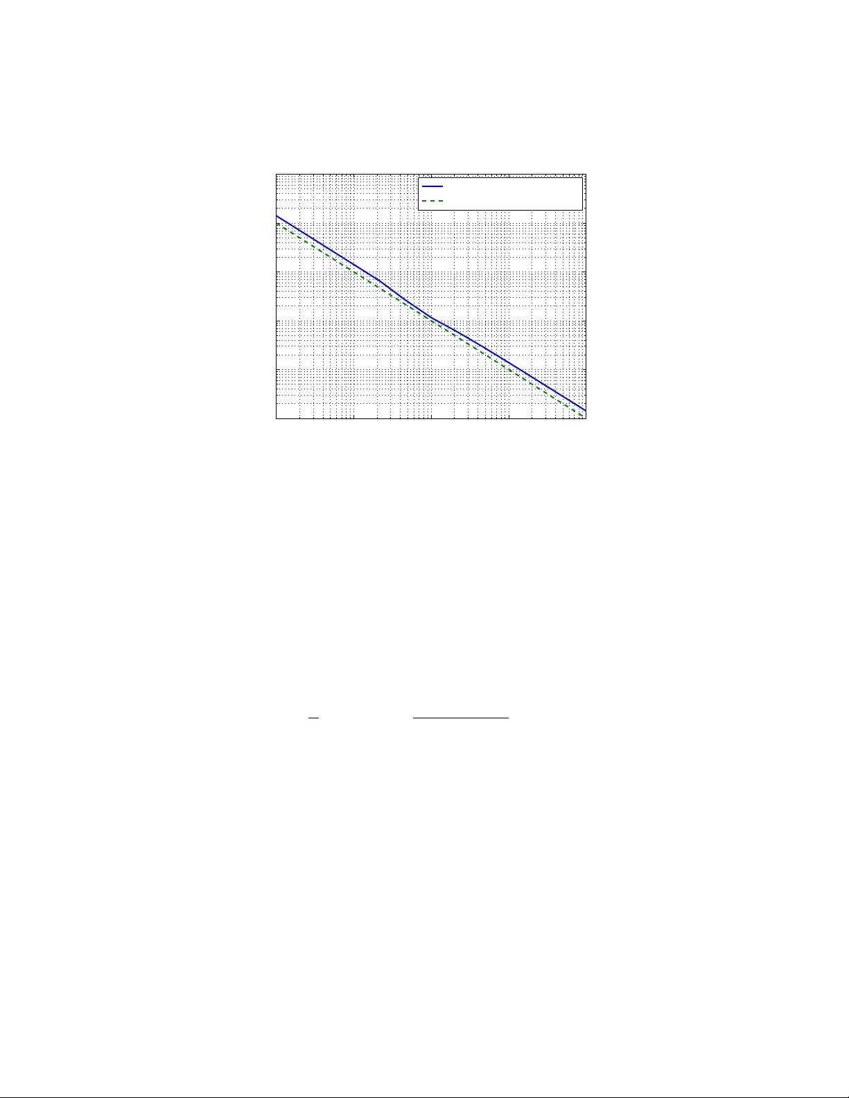
USING D A T A TO TUNE NEARSHORE D YNAMICS MODELS: A BA YESIAN APPR O A CH WITH P ARAMETRIC LIKELIHOOD NUSRET BALCI, JUAN. M. RESTREPO, AND SHANKAR C. VENKA T ARAMANI Abstract. W e propose a mo dification of a maxim um likelihoo d procedure for tuning parameter v alues in mo dels, based up on the comparison of their out- put to field data. Our methodology , whic h uses polynomial approximations of the sample space to increase the computational efficiency , differs from similar Bay esian estimation frameworks in the use of an alternativ e likelihoo d distri- bution, is sho wn to better address problems in whic h co v ariance information is lacking, than its more conven tional counterpart. Lack of cov ariance information is a frequen t c hallenge in large-scale geo- physical estimation. This is the case in the geophysical problem considered here. W e use a nearshore mo del for long shore currents and observ ational data of the same to show the contrast betw een b oth maximum likelihood method- ologies. Beyond a metho dological comparison, this study gives estimates of param- eter v alues for the bottom drag and surface forcing that make the particular model most consistent with data; furthermore, w e also deriv e sensitivity esti- mates that provide useful insights regarding the estimation procedure as well as of the model itself. Keyw ords: Polynomial Chaos, Bay esian data assimilation, maximum likeli- hoo d, parameter estimation, longshore currents, bottom drag. Submitte d to Oc e an Mo deling 1. Introduction W e hav e t wo principal goals in this work – (1) Introduce an alternative form u- lation to a maxim um lik elihoo d pro cedure for parameter estimation, whic h greatly impro ves estimates when cov ariance information of mo del and data is lac king; (2) Pro duce estimates of t w o imp ortant parameters critical to making mo del outcomes of longshore currents compatible with existing data. W e will demonstrate the prac- ticalit y and usefulness of our pro cedure by applying it to tune parameters in a mo del for nearshore dynamics using field data. W e are interested in parameter estimation for geoph ysical models which in v olv e p oten tially complex mo dels and a large n um b er of observ ations. A Ba yesian frame- w ork is natural for suc h geoph ysical problems: it is unrealistic to expect to com- pletely determine o cean states via data alone. Commonly used data assimilation metho ds for dynamic geophysical mo dels are based up on form ulating a v ariance minimizer of the posterior distribution of mo del state, giv e n observ ations (see W un- sc h (1996) for a review). The parameters are then inferred from the p osterior distribution of mo del states. F or linear/Gaussian metho ds based up on least squares, it is prudent that w e not declare the parameters as state estimation v ariables, since the ensuing state estima- tion problem is t ypically highly nonlinear and non-Gaussian. There are assimilation 1 2 NUSRET BALCI, JUAN. M. RESTREPO, AND SHANKAR C. VENKA T ARAMANI metho ds capable of dealing with nonlinearities, but these tend to b e dimensionally- c hallenged: only capable of handling problems with a small num b er of effective dynamic state v ariables ( c.f. , Restrep o (2008), Eyink et al. (2004), Stuart et al. (2004), to name a few). In the data assimilation metho ds mentioned ab ov e the p osterior is written in terms of a likelihoo d that is informed by observ ations, and a prior which is instead informed by mo del outcomes. F undamentally this presumes that mo dels and data are error-laden and most critically , that these errors are very w ell known or estimated. The parameter estimation method w e use in this w ork is the same as the methods discussed ab o ve if w e presume that the mo del is free of any errors. Alternatively , it is estimation based up on maximum likelihoo d (see Severini (2001)). In its most basic form, one writes down a likelihoo d based up on knowledge of the statistics of the errors b etw een mo dels and data. One then uses sampling metho ds to find the most likely parameters. In this w ork we are only w orking with 2 parameters so it is p ossible to circumv ent the use of Monte Carlo and instead generate a table of the likelihoo d function (plots of which will b e shown in this pap er) in sample space. Once the parameter space is mapped out, it is then straightforw ard to pick appro ximate maximum lik eliho od parameter combinations that lead to the b est compatibilit y p ossible b etw een mo del outcomes and observ ations. Whether one uses Monte Carlo or not, the computation of sample space is exceedingly exp en- siv e when geoph ysical models based on partial differential equations and/or man y equations are inv olv ed. With the aim of impro ving the efficiency of pro ducing large n umber of mo del outcomes engineering researchers hav e recently prop osed using random-co efficien t p olynomials expansions of sample mo del outcomes ( cf. , Sepah- v and et al. (2010)). W e will adopt such a strategy here. The mo del proxy will b e based upon a Polynomial Chaos expansion of the sample space ( cf. , Wiener (1938)). Demonstrations of the use of this expansion for the purpose of improving the effi- ciency of a Monte Carlo maxim um lik elihoo d parameter estimation in geophysical mo dels are found in the works of Alexanderian et al. (2012) and Sra j et al. (2013), and references contained therein. The maximum lik eliho od metho d is applied to the estimation of 2 parameters critical to nearshore longshore curren ts. W e use a vortex for c e formulation for the ev olution of w av es and currents in the nearshore (see McWilliams et al. (2004), and Lane et al. (2007)) which can capture these currents. The model was used in W eir et al. (2011) to describ e the evolution of rip curren ts. Using this mo del Uc hiyama et al. (2009) found that longshore curren t outcomes were most sensitiv ely dep enden t on the b ottom drag force (and its parametrization), and the amplitude of the incoming wa v es (whic h are b oundary conditions in the mo del). Since the drag force and the incoming w a ve forcing are such a critical part of a nearshore calculation using this wa v e/curren t mo del or some other mo del, it is essential to dev elop strategies to tune the parameter appropriately , particularly if the mo del is b eing used to explore phenomena that are less familiar than the rip currents or longshore currents. Uc hiyama et al. (2009) also found that while different b ottom drag parametriza- tions resulted in different longshore outcomes, it w as often the case that one could replicate qualitative and quan titative characteristics of the longshore curren ts with differen t models if the coefficients in the parametrization w ere c hosen appropriately . This suggests, in the setting considered, the type of parameterization is p erhaps A BA YESIAN APPRO ACH WITH P ARAMETRIC LIKELIHOOD 3 z = -h( x ) z=0 y x z z= ζ c ( x ,t) Figure 1. Schematic of the nearshore en vironment. less imp ortan t than precise tuning of the parameters for the mo del to accurately repro duce the physical outcome. W e are thus motiv ated to test the capabilities of the simplest of drag parametrizations, the linear drag force mo del, but with an accurate tuning of the parameters through comparison with field data. The data w e use was c ollected in the field campaigns conducted in Duc k, North Carolina b y Herb ers, Elgar, and Guza in 1994 (see Elgar et al. (1994)). The data sheets and detailed information is readily a v ailable on the web frf.usace.army.mil/pub/Experiments/DUCK94/SPUV . W e use the data collected in the bar region of the sea b ed top ograph y , since this is the region where w e observ e the wa v e-induced strong longshore current which the v ortex force mo del aims to capture. The pap er is organized as follows. A summary of the model app ears in Section 2. Our parameter estimation metho d using an alternative maximum likelihoo d form ulation is describ ed in Section 3. W e derive a sensitivity analysis estimate that is useful in the interpretation of mo del and observ ations. This analysis is presented in Section 4. The outcomes of the test and physical interpretation of the results app ear in Section 5. 2. The W a ve/Current Interaction Model The depth-a v eraged wa v e-curren t in teraction mo del in McWilliams et al. (2004) is sp ecialized to the nearshore environmen t. See Figure 1. The transv erse co or- dinates of the domain will b e denoted b y x := ( x, y ). The cross-shore coordinate is x and increases aw ay from the b eac h. Time is denoted by t ≥ 0. Differen- tial op erators dep end only on x and t . The total w ater column depth is giv en b y H = h ( x ) + ζ c ( x , t ), where h is the b ottom top ography and ζ c = ˆ ζ + ζ , is the comp osite sea elev ation; ˆ ζ is the quasi-steady sea elev ation adjustment, ˆ ζ = − A 2 k / (2 sinh(2 kH )), where A is the w av e amplitude and k is the magnitude 4 NUSRET BALCI, JUAN. M. RESTREPO, AND SHANKAR C. VENKA T ARAMANI of the peak wa v enum b er. In the absence of wind forcing and for spatio-temp oral scales muc h larger than those t ypical of the w av es, the momentum equation reads ∂ u ∂ t + ( u · ∇ ) u + g ∇ ζ = J + B − D + S + N , (1) where u = u ( x , t ) is the depth-av eraged transv erse velocity , g is the gravitational acceleration, J is the vortex force due to wa ves (see McWilliams and Restrep o (1999)), B is the wa v e breaking acceleration, and D is the momen tum loss due to the b ottom drag. S is the wind stress, which will b e taken to b e zero in what follo ws, as is N , whic h represents imp ortant dissipative effects from the subscale turbulen t flow. The vortex force term is defined as J = − z × u st χ, where χ is the vorticit y . W e use a linear bottom drag formulation: τ = d u . Then, the term on the right hand side of (1) is D = τ ρH , where ρ is the fluid density . The contribution to the flow due to the breaking w av es has the form B =  k ρH σ . The function  is arrived at by hydraulic jump theory . T aken from Thornton and Guza (1983)), it reads  = 24 √ π ρg B 3 r γ 4 H 5 σ 2 π A 7 , with B r = 0 . 8, γ = 0 . 4. The p eak wa ven um b er of the gravit y wa ve field k and σ the wa ve frequency ob ey the disp ersion relation σ 2 = g k tanh( k H ) . The evolution of the water column height is giv en by the contin uity equation ∂ H ∂ t + ∇ · [ H ( u + u st )] = 0 , (2) where (3) u st := ( u st , v st ) = 1 ρH W k . is the Stokes drift velocity . The ray equation for the wa v e action W := 1 2 σ ρg A 2 . is given b y ∂ W ∂ t + ∇ · ( W c ) = −  σ , (4) where c is the group velocity , given b y the formula c = u + σ 2 k 2  1 + 2 k H sinh(2 k H )  . A BA YESIAN APPRO ACH WITH P ARAMETRIC LIKELIHOOD 5 The conserv ation la w for the w av enum ber reads ∂ k ∂ t + c · ∇ k = − ( k · ∇ ) u − k σ (sinh(2 k H )) ∇ h. (5) 2.1. Mo del Computations. In the computations to b e discussed subsequen tly w e assumed that all of the fields were p erio dic in y . At the near-shore co ordinate x = x 0 , where x 0 = 100 in the particular configuration used in the numerical sim ulations, we imp osed the condition u = − u S t on the cross-shore comp onen t of the current velocity . In numerical computations, u was relaxed tow ards this b oundary conditions o v er a lay er. This la yer, h ugging the near-shore, x = x 0 side, w as selected so as to not affect the statistical comparisons and results in the region of interest. W e imp osed the homogeneous Neumann b oundary condition on ζ at x = x 0 , and we n udged ζ tow ard zero on the offshore b oundary , at x = L , where L = 600 in the n umerical sim ulations. Both W and k were prescrib ed at x = L : W is prescrib ed so as to satisfy the offshore wa v e amplitude parameter v alue. The w av e num ber was chosen to mak e an angle in the range 170 to 190 degrees, with resp ect to the shore-normal v ector, its magnitude was set once the frequency w as set. Near the shore, we imp osed p erfectly matched la y er b oundary conditions on W , whereas homogeneous Neumann b oundary condition were imp osed on k . W e used data from the exp eriments conducted by Herb ers, Guza, and Elgar, conducted in 1994, in Duck, North Carolina. W e will refer to the field data as the Duck data. The Duc k data also provides information on the mean velocity , pressure, temp erature, and depth. In addition, there is information on the p eak frequency , and b ottom topography . W e will be making use of sea elev ation data as w ell as depth-av eraged velocity data. The computational b ottom top ography , shown in Figure 2, was generated by joining their bathymetric information using a cubic spline in the cross-shore di- rection. No y v ariation was assumed for the b ottom top ography . The mo del was appro ximated using second order finite-differences in space, and Heun quadrature in time. The time steps w ere around 0 . 01 s. The computational grid was uniform. The spatial grid width in y -direction w as about 4 m (61 grid p oints are used), and in x -direction the grid width w as ab out 1 . 95 m in length and 257 grid p oints w ere used. The computational domain cov ered the cross-shore co ordinates, x , b etw een 100 m and 600 m, and was 240 m wide in the y -direction. The effective domain, whic h was largely free of effects of the relaxation and the matching lay er used in the numerical computations, encompassed shore distances from 150 m to 500 m. Among the things we know about the model, as applied to the longshore curren t problem (see Uchiy ama et al. (2009)), is that for high v alues of the drag parameter, the b ottom drag force is effectively in balance with the breaking force, and the inertial effects are largely ignorable. On the other hand, when the bottom drag parameter is small, the longshore current dev elops (non-stationary) instabilities. 3. Ba yesian Framew ork f or P arameter Estima tion The goal is to find estimates of the offshore wa v e b oundary data a := 2 A ( L, t ), where A ( x, y , t ) is the w a v e amplitude giv en by the relation W = A k (we will refer to this quan tity as the wave for cing ), and the b ottom dr ag c o efficient d that b est agree with the data. In this study , a is a b oundary condition parameter and is time-indep enden t. Sp ecifically , w e will create tables of the likelihoo d estimators for 6 NUSRET BALCI, JUAN. M. RESTREPO, AND SHANKAR C. VENKA T ARAMANI -2 0 2 4 6 8 100 200 400 600 800 1000 Depth (m) Offshore distance (m) velocity temperature sonar pressure Figure 2. The bottom topography , based up on the Duc k data. Measuremen t lo cations and the type of measurements are indi- cated. the wa v e forcing and the b ottom drag. The parameter combinations that lead to the b est agreement betw een mo del and data are the most lik ely from the table. Based up on our understanding of the ph ysics of the problem the parameter range for the wa v e forcing and b ottom drag were tak en as a ∈ [ a 0 , a 1 ] = [0 . 4 , 1 . 2] , d ∈ [ d 0 , d 1 ] =[0 . 002 , 0 . 026] , (6) resp ectiv ely . A fundamen tal assumption in the estimate (but not of the metho d itself ), is that at the times t n , n = 1 , 2 , ..., N , when data is av ailable, the statistical distribution of p − G ( q ) , is normal. Here, p ∈ R m are field measurements, q ∈ R k is the state vector. G relates the measurements and the state vector. A most common situation in geoph ysical problems, such as the longshore problem, is that m  k , and T N := min 1 ≤ n ≤ N ( t n +1 − t n ) is small compared with 1 /σ . An imp ortan t assumption used here is that correlations in time are considerably shorter than T N . In our sp ecific nearshore example, at time t n , the dimension of q is 2, times the n umber of space-grid lo cations (discoun ting for p erio dicit y and b oundary data). The measuremen t v ector p , consists of the time dependent sea elev ation and depth- a veraged velocities at measurement lo cations. G is a pro jection matrix in this problem. A BA YESIAN APPRO ACH WITH P ARAMETRIC LIKELIHOOD 7 The argument of the likelihoo d shall measure the absolute weigh ted distance b et w een data and mo del outcomes for the sea elev ation and velocities at measure- men t times t n . W e will denote the mo del output at time t n as M n . Similarly , w e will define the data v ector as O n . (The observ ation and the mo del v ectors in the argument hav e the same dimension, thanks to the implied pro jection matrix). Assuming Gaussianity in the likelihoo d, (7) P ( a, d | O ) ∝ N Y n =1 exp  − 1 2 [ M n − O n ] > R − 1 n [ M n − O n ]  U ([ a 0 , a 1 ]) U ([ d 0 , d 1 ]) , R n := R ( t n ) is a cov ariance matrix, and U [ α, β ] denotes the uniform distribution o ver the range [ α, β ]. The first term in (7) is the lik elihoo d P ( O | a, d ). The likelihoo d is a pro duct b ecause we are assuming that the distributions of the measurement errors and the model outcomes are indep endent in time. Instead of inv erting the data set to eke out the implicitly-defined mo del param- eters a and d is circumv ented by making the following assumption: the mo de of the posterior probability density for a and d given observ ations is obtained when the argument of the lik eliho o d distribution is minimized. Compared to a standard prop osal for data assimilation, (7) do es not include a prior informed by explicit mo del error indep endent of errors due to measurements. This is not to say that the mo del is error-free, but rather, that all that can be discerned is discrepancies (differ- ences) b et ween model output and measurements. In terms of parameter estimation metho dology , the maximum likelihoo d approach described ab ov e does not differ in an y significant w a y from the one prop osed by Alexanderian et al. (2012). In the next section w e will argue for an alternativ e lik eliho od function, th us distinguishing our work from theirs. 3.1. Alternativ e Ba y esian Statement. The matrix R n pro vides a description of co v ariances among the differen t comp onen ts of the state vector, the degree of confidence in eac h of these, as well as scale/non-dimensionalization information for eac h of the state comp onents. It is essential information that must b e known in order to use (7) for parameter estimation. If not supplied, one has to turn to whatever mo del and observ ations are a v ailable in order to estimate the cov ariance matrix. In fact, in geoscience applications it is often the case that the cov ariance is unknown or v ery p o orly constrained. This is the case in the longshore problem. Let M n represen t the state v ector at time t n , pro duced b y the computer-generated mo del solution, for a given set of parameter v alues, a, d . The state v ector will consist of dynamic v ariables ( e.g. , the transv erse v elo cit y and sea elev ation) at spatial lo cations with offshore x 1 , x 2 , ..., x k . The individual state vector comp onent, at time n and lo cation x j , j = 1 , ..., k , will b e denoted b y M n ( x j ) := M j n . W e will omit the sup erscript j , if it is clearly implied b y the context. M n is y -av eraged (alongshore), and time av eraged ov er times t n − 1 and t n . Because of the av eraging, we can assume that the mo del outputs give accurate estimates for the mean longshore v elo cit y for the giv en parameters at the lo cations x 1 , . . . x k . The individual component of the observ ation vector, measured at location x j , j = 1 , 2 , ..., k , will b e denoted b y O j n (again, we will omit the sup erscript j unless it is not implied b y the con text). The observ ations O n are not aver age d in y or time and hence hav e significan t v ariability . 8 NUSRET BALCI, JUAN. M. RESTREPO, AND SHANKAR C. VENKA T ARAMANI In order to remov e the dep endence on the incoming wa v e angle, we consider the magnitudes of the comp onents | O n | instead of the signed quantities O n , with the reasonable exp ectation that | O n | is comparable to | M n | . Without any other in trinsic scales in the problem, the lik eliho od, which is non-dimensional, has to be a function of | O n | / | M n | , with a distribution that is peaked when | O n | / | M n | = 1. Also, the observ ations are taken at lo cations that are sufficiently separated and on time scales which are sufficiently large that we can assume that they are uncorrelated. Th us, a natural c hoice for the lik eliho o d is L ( O n |M n , r j n ) = k Y j =1 1 Z j n exp   − 1 2( r j n ) 2 1 − | O j n | | M j n | ! 2   . where r j n is now a dimensionless measure of the v ariance of | O n | / | M n | and Z j n is a normalization given b y (8) Z j n = r π 2 | M j n | r j n  1 + erf  1 √ 2 r j n  . r j n is p otentially spatially inhomogeneous (dep ends on j ) and non-stationary (de- p ends on n ). Absent any prior information on the cov ariances, it is a reasonable appro ximation to take r j n = r , a constant. T o mak e this more precise, w e compute the Jefferys prior for r n j . The Fisher information is given b y I ( r j n | M j n ) = Z ∞ −∞  ∂ log L ∂ r j n  2 L ( O n |M n , r j n ) d O n , and is independent of M j n . This is analogous to the fact that the Fisher information for the v ariance of a Gaussian v ariable with a giv en mean is indep enden t of the v alue of the mean. W e can compute the Jefferys prior p ( r j n ) ∝ q I ( r j n ), obtaining (9) p ( r ) ∝     e − 1 r 2  2 π e 1 r 2 r 3  erf  1 √ 2 r  + 1  2 + √ 2 π e 1 2 r 2  r 2 + 1   erfc  1 √ 2 r  − 2  − 2 r  π r 5  erf  1 √ 2 r  + 1  2     1 / 2 . Figure 3 shows a comparison b et ween this prior and the scale inv ariant prior for the v ariance of a Gaussian v ariable, p G ( r ) ∝ 1 /r . As is evident from the figure, to a very goo d approximation, we ha v e p ( r ) ≈ p G ( r ) . W e now hav e the Bay esian statemen t P ( a, d, r |M , O ) ∝ p ( r ) N Y n =1 k Y j =1 1 Z j n exp  − ∆ P (1 , O j n / M j n ) 2 2 r 2  U ([ a 0 , a 1 ]) U ([ d 0 , d 1 ]) , where ∆ P ( f , g ) = min( | f − g | , | f + g | ) is the pro jective metric, and Z j n is a normalization in (8) with r j n = r . This posterior distribution generalizes (7). Note that ∆ P (1 , O j n / M j n ) = | 1 − | O j n | / | M j n || , but ∆ P has theoretically sound applications in a vectorial setup. In principle we can use this A BA YESIAN APPRO ACH WITH P ARAMETRIC LIKELIHOOD 9 1 0 − 2 1 0 − 1 1 0 0 1 0 1 1 0 2 10 − 2 10 − 1 10 0 10 1 10 2 10 3 Projective Metric Case Gaussian Approximation Figure 3. Comparison b etw een the prior giv en by (9) and the scale inv atiant prior for the v ariance of a Gaussian v ariable. to estimate the v arious momen ts of the parameters a and d and also the varianc e p ar ameter r from the mo del output and observ ations. F or the purposes of this pap er, we are only interested in computing the maximal lik eliho o d estimates for a and d and not an y of the higher moments. This allows for a further appro ximation which leads to further efficiencies in the computation. The p osterior distribution dep ends on r , through (1) the prior distribution p ( r ), (2) through the normalization factors Z n , and (3), through the denominator in the exp onen t. The logarithm of the p osterior distribution dep ends only w eakly on the first tw o factors. (So long as the size of r b e small, so that r − 2 b e large compared to log r ). With this approximation of neglecting the r dep endence except in the argumen t of the exp onen tial function, the posterior distribution reduces to (10) P ( a, d | O ) ∝ 1 Z N Y n =1 k Y j =1 exp  − ∆ P (1 , O j n / M j n ) 2 2 r 2  U ([ a 0 , a 1 ]) U ([ d 0 , d 1 ]) , where ∆ P is the pro jectiv e metric defined ab o ve and Z is a normalization constant. In our computations, the v ariance parameter r in the lik eliho od function is set to 2. As is eviden t from (10), changing r will only c hange the width of the empirical lik eliho o d, but not the v alue of maxim um likelihoo d estimates. Figure 4 illustrates the difference b et ween using absolute errors and relative errors. The striking difference is that there is clearer discernmen t of likely parameter v alues (pure black represents the most lik ely). The differences p ortray ed here are v ery drastic in this case, but this sharp ening due to the use of the relativ e error is a generic outcome of the computations 3.2. P olynomial Expansion of the Parameter Sample Space. In a many- parameter estimation problem we would apply a Mon te Carlo pro cedure to sample parameter space (see Kroese et al. (2011)). F ull mo del sim ulations mak e this aspect of the metho dology computationally demanding. Whether we hav e to use Mon te 10 NUSRET BALCI, JUAN. M. RESTREPO, AND SHANKAR C. VENKA T ARAMANI (a) 0.4 0.5 0.6 0.7 0.8 0.9 1 1.1 1.2 a 0.005 0.01 0.015 0.02 0.025 d 0 0.2 0.4 0.6 0.8 1 (b) 0.4 0.5 0.6 0.7 0.8 0.9 1 1.1 1.2 a 0.005 0.01 0.015 0.02 0.025 d 0 0.1 0.2 0.3 0.4 0.5 0.6 0.7 0.8 0.9 1 Figure 4. A daily comparison for Octob er 7-8. (a) Posterior us- ing absolute errors. See (7); (b) lik elihoo d based upon the relativ e errors. See (10). The latter suggests that a muc h sharp er range of parameters leads to agreemen t b etw een model and data. Carlo or not the efficiency of this process can b e considerably improv ed b y using a parametric approximation of the model outcomes, via polynomial chaos expansions (see Alexanderian et al. (2012)). The p olynomial chaos expansion of a sto chastic function f ( x , t, η ) of one sto- c hastic parameter η is F K = K X k =0 P k ( η ) f k ( x , t ) , where { P k } K k =0 is a system of orthogonal p olynomials of degree k , 0 ≤ k ≤ K . Orthogonalit y is with resp ect to the probabilit y distribution of the parameter η . If the distribution is uniform, for example, the P k are Legendre p olynomials. F or t wo parameters, the basis consists of p olynomials { P k ( η ) Q m ( ξ ) } k = K,m = M k =0 ,m =0 , and the p olynomial approximation is F K M = K X k =0 M X m =0 P k ( η ) Q m ( ξ ) f km ( x , t ) . A BA YESIAN APPRO ACH WITH P ARAMETRIC LIKELIHOOD 11 Exploiting the orthogonality of the p olynomials, we can easily find the co efficien ts f k 0 m 0 : W e multiply F K M b y P k 0 Q m 0 and integrate ov er η and ξ with resp ect to the known joint measure η and ξ . In our case, this distribution is just a constant m ultiple of the Leb esgue measure. F or the integration, we chose a simple Romberg integration. How ev er, there are more efficient or accurate quadrature schemes, e.g. , Gaussian quadrature or Smoly ak tensorisation (see Alexanderian et al. (2012) and references contained therein). 3.3. Computational Efficiency of the Pro cedure. W e chose not to resort to Mon te Carlo, since our parameter sample space is tw o-dimensional. Instead, we opted to discretize sample space in the range given b y (6) with an equally spaced grid consisting of 256 2 v alues. In pro ducing appro ximations to o ceanic flo ws with numerical mo dels there is a computational exp ense of O ( N d × T ), where N is the state v ariable dimension, d is the n umber of spatial dimensions (typically 2, lately 3), and T is the n umber of time steps in the computation. N is up w ards of 10 5 , typically . Most co des are explicit in time, and th us T = c N due to stability constrain ts, where c is a constant. In the n umerical computations that will b e describ ed subsequen tly we mention that after the initialization, the mo del w as run for 20 model minutes, and the last 11 minutes of the mo del output was av eraged in time and in the y -co ordinate to pro duce reference mo del output. On a 2.66 GHz dual-core machine a single model sim ulation to ok approximately 25 wall-clock min utes to complete. If we did not rely on the Legendre p olynomial expansion, the cost of the compu- tation w ould hav e b een 256 2 × O ( N d × T ). How ev er, with the aid of the Legendre p olynomial expansion we required 17 runs, to cov er the wa ve forcing a parameter range, and 33 runs to cov er the drag parameter d range. Th us, there w ere 17 × 33 full-scale runs. Once these are p erformed, generating a 256 2 grid of parameter- space runs had a trivial computational exp ense. In terms of wall-clock time the Legendre calculation was about 117 times faster than the direct ev aluation of the 256 2 mo del runs. 4. Sensitivity of the Longshore Current with Respect to the Drag F orce The mono chromatic w a ve description used in the mo del, allows us to relate the field observ able RMS wa v e height, H rms , to the wa v e action W through the w a ve amplitude A (by taking H rms = 2 A ), and k the sp ectrum p eak wa ven um b er. W e use a Reynolds decomposition: F or f ( x, y , t ), we write f = h f i + f 0 , where h f 0 i ≈ 0. The angle brac k ets denote the av eraging in time and in the y - direction. Assuming steady wa v es and currents, av eraging in the x -direction yields h u i = −h u st i , namely , the anti-Stok es condition. The mean momentum equation in the y -direction, is then (11) h u i ∂ h v i ∂ x + h u 0 ∂ v 0 ∂ x i + h u st ih χ i + h u st 0 χ 0 i + d h v H i − h B y i = 0 . 12 NUSRET BALCI, JUAN. M. RESTREPO, AND SHANKAR C. VENKA T ARAMANI If the flow is steady , as is known to b e the case for large b ottom drag v alues, we obtain the balance (12) d h v H i = h B y i . W e recall the definition of B = ( B x , B y ) =  b k ρH σ , and thus (13) d h v H i = const h k 2 H 7 rms H 6 i . As remarked at the op ening of the section, H rms can is related to the wa v e ampli- tude in a simple and linear relation. The wa ve amplitude is determined mainly by the offshore w a v e amplitude up until the breaking zone where the relativ ely strong alongshore curren t is generated. W e therefore relate H rms to the offshore wa ve forcing a , a b oundary-v alue parameter in our numerical computations, in a linear fashion: i.e. , we mak e a first order appro ximation. Next w e assume that the impact of a small change in d on k 2 and H are negligible. This assumption is supp orted b y the numerics. Ho w ev er, when we change d , to satisfy the balance in (13) and assumptions leading to it, w e ha v e to change the other main parameter, the offshore w av e forcing, as well. This will c hange the mean longshore velocity , as a result. W e th us obtain (14) ( d + ∆ d ) h v + ∆ v i ≈ const ( H , k 2 )( H rms + ∆ H rms ) 7 , and (15) d h v i ≈ const ( H , k 2 ) H 7 rms . Subtracting the tw o relation, for small ∆ d (and we assume this results in infitesimal c hange to H rms to achiev e the balance in (13)), gives h ∆ v i ≈ const ( H , k 2 , H rms ) ∆ H rms d + ∆ d . W e further restrict ourselves to the case where d is aw a y from zero and relatively large compared to the increment ∆ d . Th us, by the aforementioned linear appro xi- mation of H rms using the b oundary wa v e forcing parameter a , we conclude that (16) h ∆ v i ≈ const ( H , k 2 , H rms ) ∆ a d . The parameter estimation results that follow in the next section m ust reflect this dep endency . 5. Resul ts There are a v ariet y of drag force parametrizations, but here we wan t to sp ecif- ically test the linear drag mo del. Such a mo del asserts that the drag force is prop ortional to the lo cal depth-av eraged velocity via the constant d . The drag force is thus only time dep enden t via the velocity itself. W e then exp ect that the maxim um likelihoo d estimation should b e very stable to c hanges in the drag force parameters. In con trast, w e can exp ect higher v ariability in the forcing amplitude. In Section 4 w e derived the structural reasons in the mo del that lead to this type of sensitivity . In our study , w e compare the longshore depth-a veraged, time-av eraged, and spatially y -a v eraged velocity comp onent predicted by the mo del with the mean A BA YESIAN APPRO ACH WITH P ARAMETRIC LIKELIHOOD 13 longshore current rep orted by Herb ers, Guza, and Elgar from exp erimen ts con- ducted in 1994, in Duck, North Carolina. The collected data, is av ailable from www.frf.usace.army.mil/duck94/duck94.stm . The exp erimen tal data we use here were collected by the devices v12, v13, v14, which were lo cated approximately at the offshore co ordinates 205, 220, and 240 m, resp ectiv ely . These devices lo- cations cov er the bar region of the domain which has stronger mean longshore curren ts. A plot sho wing the device lo cations as w ell as a snapshot of the b ottom top ograph y app ears recreated in Figure 2. The longshore current data in this exp eriment was collected at a sampling rate of 2 Hz, every 1024 s. There are ov er 5000 suc h data sets, spanning the months of September, Octob er, and early Nov em b er. A small p ortion of the data w as not used, either b ecause there was a device failure or b ecause the datum w as an extreme outlier. Since there were sev eral exp eriment al devices with approximately the same longshore co ordinate, mo del output as well as instrumental data was y -av eraged. As a result, the mo del-data discrepancy has no longshore dep endence. The month of Septem b er, Octob er, and Nov em ber observ ations include 5030 data p oin ts for the longshore mean current. First 2370 data p oin ts come from the observ ations in Septem b er 1994, the next 2450 from October 1994, the last 210 in Nov em b er 1994. In the text, w e num ber these data p oints consecutiv ely . The general outcomes can b e summarized as follo ws: • The prop osed lik eliho od w as sup erior to the more traditional, absolute dis- tance likelihoo d, giv en that there was no cov ariance information av ailable. In particular, it delivered sharp er maximally-likely parameter v alues for mo del/data agreement. • With regard to the p olynomial chaos expansion, we found that the first few terms in the sequence were of significance in all the cases considered: F or the wa v e forcing amplitude a w e use the first 6 co efficients, whereas for the drag co efficien t d we used the first 9 coefficients. W e found that using more co efficien ts did not significan tly improv e the results. • The use of the p olynomial chaos expansion impro ved the efficiency of the parameter estimation by 2 orders of magnitude. • W e found that the most lik ely wa v e forcing was in the range, a = 0 . 8 − 1 . 1 m. The most lik ely b ottom drag coefficient was in the range d = 0 . 007 − 0 . 020. The mo del is thus most consisten t with the data when w a ve amplitudes are large, but not excessively so, and in the range of dynamics wherein the attractor of solutions reflects a balance of breaking and drag forces and near-steady longshore currents. • With regard to the length of the experiments, we found that a minimum of 3-5 hours of data w ere needed. Among the reasons for this is that b elow 3 hours the num ber of time records w ere to o few: less than tw elve. • When several 3 hour data exp erimen ts were compared, we found v ariations in the wa v e forcing estimate. This is a p ositiv e mo deling outcome: v aria- tions in the w a v e forcing are tied to the time scales of wind v ariation, which is roughly 3-6 hours. Figure 5 is typical of estimates at different times of the da y . The times of these observ ations are September 25, 16:51-19:51 and Septem b er 25-26, 23:59-3:16. • On the other hand, we found that the drag co efficient w as not as sensitiv e to the length of the exp erimen t: Whether using 3 hour or daily data, the 14 NUSRET BALCI, JUAN. M. RESTREPO, AND SHANKAR C. VENKA T ARAMANI (a) 0.4 0.5 0.6 0.7 0.8 0.9 1 1.1 1.2 a 0.005 0.01 0.015 0.02 0.025 d 0 0.1 0.2 0.3 0.4 0.5 0.6 0.7 0.8 0.9 1 (b) 0.4 0.5 0.6 0.7 0.8 0.9 1 1.1 1.2 a 0.005 0.01 0.015 0.02 0.025 d 0 0.2 0.4 0.6 0.8 1 Figure 5. Three-hour comparisons of data and mo del output. (a) Posterior for data points 1944 through 1955; a comparison p er- formed starting 3 hours later, (b) another three-hour posterior for data p oints 1968 through 1979. W e note that the wa ve forcing c hanges significantly , but not the drag. Nev ertheless, the results are reasonable, and the metho dology p ermits trac king this c hange in parameter estimates. (a) 0.4 0.5 0.6 0.7 0.8 0.9 1 1.1 1.2 a 0.005 0.01 0.015 0.02 0.025 d 0 0.2 0.4 0.6 0.8 1 (b) 0.005 0.01 0.015 0.02 0.025 0.4 0.5 0.6 0.7 0.8 0.9 1 1.1 1.2 d a 0 0.1 0.2 0.3 0.4 0.5 0.6 0.7 0.8 0.9 1 Figure 6. Relatively stronger wa v e heights induce similar daily p osteriors with more spread out mo des. W e note the steep curve traced b y the most lik ely parameter v alues, with large v ariabilit y in the bottom drag, and less v ariability in the forcing amplitude. The maxim um likelihoo d curv e in parameter space, asso ciated with the lik eliho o d function is shown in Figure 6b. The estimate in (17) qualitativ ely conforms with the curve. results were similar, with relatively high b ottom drag co efficients fav ored; nev ertheless, sligh tly larger than 0.007, the marginally stable v alue used in Uc hiyama et al. (2009). F or the daily runs, partitions of 96 consecutive data p oints in the observ ations were used. In Figure 6 we sho w a ”daily” case, from September 1. A BA YESIAN APPRO ACH WITH P ARAMETRIC LIKELIHOOD 15 0.4 0.5 0.6 0.7 0.8 0.9 1 1.1 1.2 a 0.005 0.01 0.015 0.02 0.025 d 0 0.2 0.4 0.6 0.8 1 Figure 7. The Bay esian p osterior is at o dds with what we know ab out the physics of longshore currents. Data p oints 3800 through 3895 are c haracterized by the presence of v ery strong curren ts. The mo del is unable to capture the data. • T racing the maximum lik elihoo d curve in a × d parameter space (see Figure 6) w e obtain a curve, which when combined with (16), recov ers a semi- empirical law whic h holds for our case of interest: (17) h ∆ v i ∼ H,k 2 ,H rms ∆ d d . In obtaining this relationship we assumed that ∆ H rms ≈ const × ∆ d . This semi-empirical relationship says that the mean longshore v elo cit y in the balance (13) dep ends on the drag parameter in a lo cally logarithmic manner. This is consisten t with the shap es of the posterior distributions, and the numerical observ ations in the sample runs: the higher the drag, the lesser the impact of the c hange in the drag on the v elocity field. This is particularly evident in Figure 6b, which highligh ts the maximum lik eliho od curv e in parameter space, corresp onding to data p oin ts 700 through 795. The tuning strategy is not failure-pro of, but this is not seen here in a negative ligh t: If the mo del and the data are irreconcilable it is p ossible for one to obtain estimates that make little sense. That we kno w they do not mak e sense means that w e know something ab out the physics and limitations of the mo del for us to make this determination. W e do not hav e this m uch knowledge ab out the outcomes in other complex problems. F or models that are exceedingly complicated this b ecomes a nontrivial challenge. Nevertheless, priors can b e used to narro w the parameter searc h or for constraining its c haracteristics: More priors can b e embedded in to (10). The danger, ho w ever, is that these priors inform the p osterior to o strongly; what is desired is that the priors inform the likelihoo d. A non-sensical case is sho wn in Figure 7, using a data set corresp onding to measurements 3800 through 3895. This is a daily-data exp eriment suggesting that the likely drag v alues are exceedingly small and the w av e forcing very high. Mo del outcomes corresp onding to this case would corresp ond to highly unstable modeled longshore currents with v ariability that is not consisten t with measurements. 16 NUSRET BALCI, JUAN. M. RESTREPO, AND SHANKAR C. VENKA T ARAMANI 6. Summar y W e prop osed an alternativ e maximum likelihoo d function for mo del/data dis- parit y for parameter estimation, suitable in cases when co v ariance information is una v ailable or p o orly constrained. The lack of this information frequen tly o ccurs in real-w orld applications and th us it is argued that this alternativ e lik elihoo d function will hav e practical v alue. The cov ariance matrix not only pro vides weigh ts for mo del/data disparity . It is also crucial in nondimensionalizing and setting prop erly the scales of the state v ector. If the state vector is comp osed of m ulti-ph ysics comp onents, the lack of scale information might become an unsurmoun table c hallenge in practical parame- ter estimation. One could non-dimensionalize the state vector in the mo del and the data, but doing so in a large scale model (or in an existing co de that approximates solutions to the mo del) can b e impractical. Moreov er, even if there is no m ulti- ph ysics, but rather, a multiplicit y of spatio-temp oral scales, the challenge will not b e easily obviated b y a fixed scaling. With regard to parameter estimation we show ed that using the traditional max- im um likelihoo d v arian t (presuming no cov ariance information is kno wn), pro duces parameter estimates that can b e v ague, or at w orst, uninformative. The alterna- tiv e maximum likelihoo d function replaces the weigh ted mo del/data disparity , the absolute error, by a relative error b et ween these. In doing so we make sure that the likelihoo d function will automatically adjust in a reasonable wa y its v ariance according to the scales of the state vector comp onents (and of its spatio-temp oral c haracteristics). The use of the relativ e error will make larger demands with regard to the compatibility of the observ ations and the mo del based up on the importance, in terms of magnitude, of the mo del state vector. This leads to sharp er estimates. This is not generally the case when the absolute error is used: discrepancies b etw een mo del output and observ ations are not ordered with regard to their imp ortance, unless judiciously done so in an ad-ho c fashion. A lik eliho od whic h is cast in terms of the relative error changes the issue of the relative confidence of the individual elemen ts of the absolute error to one in terms of relative error c hanges. That is, one is now required to know the dimensionless measure of the v ariance of the rel- ativ e size of measurements to mo del outcomes. Under reasonable assumptions the Jeffreys prior can b e used to justify the replacement of each dimensionless measure of the v ariance by a single constant. Large-scale dynamics mo dels make parameter estimation extremely c hallenging, due to the curse of dimensionality: firstly , b ecause of the combinatoric complexity of c ho osing parameters within a mo del, and secondly , b ecause the mo dels tend to ha ve many degrees of freedom. In our case, we only had 2 parameters and th us w e did not ha v e to resort to Monte Carlo and exp erimental design. F or the latter, the adoption of a Legendre p olynomial approximation to the mo del output increased the efficiency of parameter estimation one-hundred-fold. W e also derived an estimate of the parameter dep endence, betw een the drag and the w av e forcing; namely , the rate of v ariability of the mo del outcomes to c hanges in these tw o parameters (see (16)). W e used this estimate to v erify that the likelihoo d estimates, derived using our new formulation were qualitativ ely correct. The longshore problem has at least tw o qualitatively different flo w regimes. Ac- cording to the model, the mo del trac ks the Duck data in a flo w regime wherein the drag forces and the breaking wa v e forces are in a near-balance and the longshore A BA YESIAN APPRO ACH WITH P ARAMETRIC LIKELIHOOD 17 curren t nearly steady; in that regime we found likely parameter combinations. The sensitivit y of the parameters in the estimation reflected well a theoretical estimate of their relative v ariabilit y , derived from the mo del itself. The linear drag mo del w as v alidated in this steady-longshore flo w regime. It should b e noted that the data did not lend itself to ev aluating the drag mo del in the more time-unstable flo w regime. A cknowledgments W e received funding from GoMRI/BP . JR and SV also received funding from NSF-DMS-1109856. This work was supp orted in part b y the National Science F oundation under Grant No. PHYS-1066293 and the hospitality of the Asp en Cen ter for Physics. JR wishes to thank Andrew Stuart, for stim ulating discussions, as well as the American Institute of Mathematics. References Alen Alexanderian, Justin Winokur, Ihab Sra j, Ashw an th Sriniv asan, Mohamed Isk andarani, William C. Thack er, and Omar M. Knio. Global sensitivity analysis in an o cean general circulation mo del: a sparse sp ectral pro jection approac h. Computational Ge oscienc e , 16:757–778, 2012. doi: 10.1007/s10596- 012- 9286- 2. S. Elgar, T. H. C. Herb ers, and R. T. Guza. Reflection of o cean surface gra vity w av es from a natural b eac h. Journal of Physic al Oc e ano gr aphy , 24:1503–1511, 1994. G. L. Eyink, J. M. Restrep o, and F. J. Alexander. A mean field appro ximation in data assimilation for nonlinear dynamics. Physic a D , 194:347–368, 2004. D. P . Kroese, T. T aimre, and Z. I. Botev. Handb o ok of Monte Carlo Metho ds . John Wiley and Sons, New Y ork, 2011. E. M. Lane, J. M. Restrep o, and J. C. McWilliams. W a ve-curren t interaction: A comparison of radiation-stress and vor tex-force representations. Journal of Physic al Oc e ano gr aphy , 37:1122–1141, 2007. J. C. McWilliams and J. M. Restrep o. The wa ve-driv en o cean circulation. Journal of Physic al Oc e ano gr aphy , 29:2523–2540, 1999. J. C. McWilliams, J. M. Restrep o, and E. M. Lane. An asymptotic theory for the in teraction of w av es and currents in coastal waters. Journal of Fluid Me chanics , 511:135–178, 2004. J. M. Restrep o. A path integral metho d for data assimilation. Physic a D , 237: 14–27, 2008. K. Sepahv and, S. Marburg, and H. J. Hardtke. Uncertaint y quantification in sto- c hastic systems using p olynomial chaos expansion. International Journal of Ap- plie d Me chanics , 2:305–353, 2010. Thomas A. Severini. Likeliho o d Metho ds in Statistics . Oxford Universit y Press, New Y ork, 2001. Ihab Sra j, Justin Winokur, Alen Alexanderian, Chia-Ying Lee, Shuyi S. Chen, Ash wan th Sriniv asan, Mohamed Isk andarani, William C. Thack er, and Omar M. Knio. Bay esian inference of wind drag dependence on w ind sp eed 2 using AXBT data during Typho on Fanapi. Oc e an Mo deling , 2013. A.M. Stuart, J. V oss, and P . Wib erg. Conditional path sampling of SDEs and the Langevin MCMC metho d. Communic ations in the Mathematic al Scienc es , 2:685–697, 2004. 18 NUSRET BALCI, JUAN. M. RESTREPO, AND SHANKAR C. VENKA T ARAMANI E. B. Thornton and R. T. Guza. T ransformation of w a v e height distribution. Jour- nal of Ge ophysic al R ese ar ch , 88 (C10):5925–5938, 1983. Y. Uchiy ama, J. C. McWilliams, and J. M. Restrep o. W av e-current interaction in nearshore shear instabilit y analyzed with a Vortex Force formalism. Journal of Ge ophysic al R ese ar ch , page C06021, 2009. doi: doi:10.1029/2008JC005135. B. W eir, Y. Uc hiyama, E. Lane, J. M. Restrep o, and J. C. McWilliams. A Vortex Force analysis of the in teraction of rip curren ts and surface gra vit y wa v es. Journal of Ge ophysic al R ese ar ch , 116:C050001, 2011. N. Wiener. The homogeneous chaos. Americ an Journal of Mathematics , pages 897–936, 1938. C. W unsch. The Oc e an Cir culation Inverse Pr oblem . Cambridge Univ ersity Press, Cam bridge, UK, 1996. Dep ar tment of Ma thema tics, University of Arizona, Tucson, AZ 85721, USA. E-mail address : shankar@math.arizona.edu Dep ar tment of Ma thema tics, University of Arizona, Tucson, AZ 85721, USA. E-mail address : restrepo@math.arizona.edu Dep ar tment of Ma thema tics, University of Arizona, Tucson, AZ 85721, USA. E-mail address : shankar@math.arizona.edu