Outlying Property Detection with Numerical Attributes

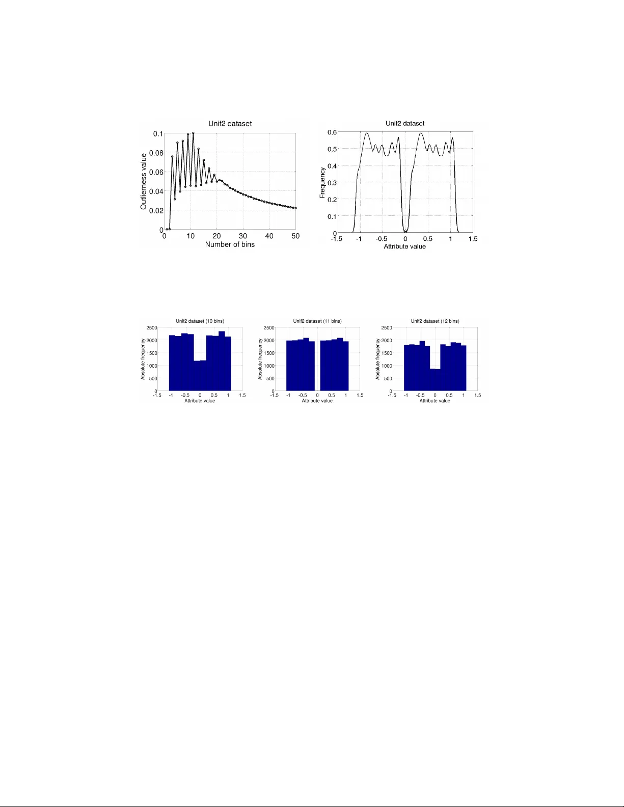
Outlying Prop ert y Detection with Numerical A ttributes F abrizio Angiulli 1 , F abio F assetti 1 , Giusepp e Manco 2 , and Luigi P alop oli 1 1 DIMES Dept., Univ ersity of Calabria, Rende, Italy { f.angiulli,f.fassetti,palopoli } @dimes.unical.it 2 ICAR-CNR, Rende, Italy manco@icar.cnr.it Abstract. The outlying pr op erty dete ction pr oblem is the problem of disco vering the prop erties distinguishing a given ob ject, known in ad- v ance to b e an outlier in a database, from the other database ob jects. In this pap er, w e analyze the problem within a con text where numerical attributes are taken into accoun t, which represents a relev ant case left op en in the literature. W e introduce a measure to quan tify the degree the outlierness of an ob ject, whic h is associated with the relativ e likelihoo d of the v alue, compared to the to the relativ e lik eliho od of other ob jects in the database. As a ma jor contribution, we present an efficient algorithm to compute the outlierness relativ e to significan t subsets of the data. The latter subsets are characterized in a rule-based fashion, and hence the basis for the underlying explanation of the outlierness. 1 In tro duction In this w ork we aim at char acterizing outliers. Outliers are the exc eptional ob- jects in the input dataset, that is to say ob jects that significan tly differ from the rest of the data. Approaches to outlier detection introduced in the literature can b e classified in supervised [11], which exploit a training set of normal and ab- normal ob jects, semi-sup ervised [22], which assume that only normal examples are given, and unsup ervised [8, 17, 9, 21, 7, 3, 20, 4, 10], whic h search for outliers in an unlab elled data set. It is w orth to notice that the abov e men tioned methods focus only on identifi- c ation , and they do not concen trate on pro viding a description or an explanation of wh y an identified outlier is exceptional, which is vice versa the problem we are intended to face here. While outlier detection in datasets has b een one of the most widely inv estigated problems in data mining, the related problem of outlier explanation receiv ed less attention in the literature. It m ust b e noticed that the outlier explanation problem is completely different from sup ervised and semi-sup ervised outlier detection, and, moreo ver, is to b e considered orthogonal to the unsup ervised outlier detection task. As an example of outlier explanation task, assume y ou are analyzing health parameters of a sic k patien t, whic h include several features such as bo dy temper- ature, blo od pressure measuremen ts and others. If an history of health y patients is av ailable, then it is relev ant to single out those parameters that mostly differ- en tiate the sic k patient from the healthy p opulation. It is imp ortan t to highligh t here that the abnormal individual, whose p eculiar characteristics we wan t to detect, is provided as an input to the outlier explanation problem, that is, this individual has b een recognized as anomalous in adv ance by the virtue of some external information, mean or pro cedure. The fo cus of this pap er is the discov ery of outlying pr op erties : we are in- terested in unv eiling the hidden structures that mak e an input outlier ob ject o sp ecial w.r.t. an input population. This can be accomplished ( i ) by detecting the subsets S of the input p opulation that represen t an homogeneous sub-p opulation, in tuitively a set of ob jects sharing similar features (whic h w e will refer to as ex- planations ), including o , and ( ii ) b y identifying attributes (also referred to as pr op erties ) where o substan tially differentiates from the other ob jects in S . With this aim, subspace outlier mining tec hniques, like the one presented in [1], could in principle b e used to extract information ab out outlier prop erties. Ho wev er, the originary task considered in [1] is differen t from the task inv es- tigated here, since subspaces therein highlight the outlierness, whereas in our approac h they represent an homogeneous subp opulation upon which to compare a given prop erty . In [18], the authors fo cus on the identification of the inten- sional knowledge asso ciated with distance-based outliers. How ever, this setting mo dels outliers which are exceptional with resp ect to the whole p opulation, but it do es not capture ob jects that are exceptional only if compared to homo- geneous subp opulations. In [6] an outlier subp opulation is given in input and compared with the inlier population in order to simultaneously characterize the whole exceptional subp opulation. Despite the latter approach shares with ours a common rationale, we note that the framework considered in [6] is differen t and the solutions there prop osed cannot b e applied to the special case in which the outlier sub-p opulation consists of just one single individual, which is precisely the scenario considered here. A viable solution to the outlying prop ert y detection problem has b een de- vised in [5]. Specifically , a set of attributes witnesses the abnormalit y of an ob ject if the combination of v alues the ob ject assumes on these attributes is v ery in- frequen t with resp ect to the ov erall distribution of the attribute v alues in the dataset, and this is measured my means of the so called outlierness score. A ma jor problem with the outlierness score presented in [5] is that it w as sp ecifi- cally designed and shown effective for categorical attributes. Hence the question is how to adapt that idea to a more general setting with both categorical and n umerical attributes. W e point out that discretizing numerical attributes and applying the tec hnique of [5] to the discretized attributes is not a suitable so- lution, for several reasons. First of all, the result of the analysis will strongly dep end on the results of the discretization pro cess. This drawbac k is further exacerbated by the p eculiarities of the outlierness measure, whic h assigns higher scores to very unbalanced distributions, and b y contrast provides low scores to uniform frequency distributions. In a sense, the discretization process should be sup ervised b y the outlierness score, in order to detect in the first place the bins capable of magnifying the score itself. The appropriate treatment of n umerical attributes is indeed one of the main problems we deal with in this pap er. Sp ecifically , the main contribution of this w ork amounts to provide an outlierness measure representing a refined general- ization of that prop osed in [5] and which is able to quan tify the exceptionality of a given n umerical or categorical pr op erty featured by the given input anomalous ob ject with resp ect to a reference data p opulation. In particular, in order to quan tify the degree of unbalanceness b et ween the frequency of the v alue under consideration and the frequencies of the rest of the database v alues, our mea- sure analyzes the curv e of the cum ulativ e distribution function ( c df ) asso ciated with the o ccurrence probabilit y of the domain v alues. It is worth noting that relying on the c df allows to correctly recognize exceptional prop erties indep en- den tly of the form of the underlying probability densit y function ( p df ), since the former compares the o ccurrence probabilities of the domain v alues rather than directly comparing the domain v alues themselv es. This enables us to build a gen- eral metho dology for uniformly mining exceptional properties in the presence of b oth categorical and n umerical attributes, so that a fully automated supp ort is pro vided to deco de those prop erties determining the abnormality of the given ob ject within the reference data context. The rest of the pap er is organized as follo ws. Section 2 in tro duces the outlier- ness measure and the concept of explanation. Section 3 describ es the metho d for computing outlierness and determining asso ciated explanations. Section 4 dis- cusses exp erimen tal results. Finally , Section 5 presen ts conclusions and discusses future w ork. 2 Outlierness and Explanations T o b egin with, we fix some notation to b e used throughout the pap er. In the follo wing, a denotes an attribute , that is an iden tifier with an asso ciated domain D ( a ), and A = a 1 , . . . , a m denotes a set of m attributes. The value v i asso ciated with the attribute a i in the ob ject o will be denoted by o [ a i ]. A datab ase DB on a set of attributes A is a m ulti-set of ob jects on A . W e shall characterize p opulations in a “rule-based” fashion, by denoting the subset of DB that embo dies them. F ormally , a c ondition on A is an expression of the form a ∈ [ l , u ], where ( i ) a ∈ A , ( ii ) l , u ∈ D ( a ), and ( iii ) l ≤ u , if a is numeric, and l = u , if a is categorical. If l = u , the in terv al I = [ l , u ] is sometimes abbreviated as u and the condition as a ∈ I or a = I . Let c b e a condition a ∈ [ l, u ] on A . An ob ject o of DB satisfies the condition c , if and only if o [ a ] equals l , if a is categorical, or l ≤ o [ a ] ≤ u , if a is numerical. Moreo ver, o satisfies a set of conditions C if and only if o satisfies eac h condition c ∈ C . Giv en a set C of conditions on A . The sele ction DB C of the database DB w.r.t. C is the database consisting of the ob jects o ∈ DB satisfying C . Next, the definitions of outlierness and explanation are in tro duced. 2.1 Outlierness This measure is used to quan tify the exceptionalit y of a property . The intuition underlying this measure is that an attribute makes an ob ject exceptional if the relativ e lik eliho od of the v alue assumed by that ob ject on the attribute is rare if compared to the relativ e lik eliho o d associated with the other v alues assumed on the same attribute b y the other ob jects of the database. Let a b e an attribute of A . W e assume that a random v ariable X a is asso ciated with the attribute a , whic h mo dels the domain of a . Then, with f a ( x ) we denote the pdf asso ciated with X a . The pdf pro vides a first indication on the outlierness degree of a giv en v alue x , as usually w e w ould expect lo w pdf v alues asso ciated to outliers. Ho wev er, the sole pdf v alue is not enoughs. A giv en pdf v alue represen ts a hypothetical “frequency” for that v alue in the sample under consideration. How t ypical is that “frequency” pro vides a b etter insigh t on the outlierness degree: a lo w p df v alue in a p opulation exhibiting low v alues only is not an indicator of an outlier, whereas an anomalous low p df v alue in a p opulation of significantly higher v alues denotes that the v alue under observ ation represents an outlier. Th us, analyzing ho w the v alues distribute on a p df is the key for measuring the degree of outlierness. Let X f a denote the random v ariable whose p df represents the relative likeli- ho od for the p df f a to assume a certain v alue. The cdf G a of X f a is: G a ( f ) = Z f 0 P r ( X f a ≤ f ) d f . (1) Example 1. Assume that the height of the individuals of a p opulation is normally distributed with mean µ = 170 cm and standard deviation σ = 7 . 5 cm . Then, let a b e the attribute representing the heigh t, X a is a random v ariable following the same distribution of the domain and f a ( x ) is the asso ciated p df, reported in the first graph of fig. 1. The p df f a ( x ) assumes v alue in the domain [0 , f a ( µ ) = 0 . 0532] ⊂ R . Consider, no w, the random v ariable X f a . The cdf G a ( v ) associated with X f a denotes the probability for f a to assume v alue less than or equal to v . Then, G a ( v ) = 0 for eac h v ≤ 0 and G a ( v ) = 1 for eac h v ≥ 0 . 0532. T o compute the v alue of G a ( v ) for a generic v , the integral rep orted in Equation (1) has to b e ev aluated. The resulting function is rep orted in the second graph of fig. 1. The outlierness out a ( o, DB ) (or, simply , out a ( o )) of the attribute a in o w.r.t. DB is defined as follows: out a ( o ) = Ω Z + ∞ f a ( o [ a ]) (1 − G a ( f )) d f − Z f a ( o [ a ]) 0 G a ( f ) d f ! , (2) where Ω denotes a suitable function mapping R to [0 , 1] such that ( i ) Ω ( x ) = 0 for x < 0, and ( ii ) Ω is monotone increasing for x ≥ 0. In the following w e emplo y the mapping Ω ( x ) = 1 − exp( − x ) 1 + exp( − x ) . Fig. 1. Example of function G a ( · ). The first in tegral measures the ar e a ab ove the cdf G a ( f ) for f > f a ( o [ a ]), while the second in tegral measures the ar e a b elow the cdf G a for f ≤ f a ( o [ a ]). Intu- itiv ely , the larger the first term, the larger the degree of unbalanceness b etw een the occurrence probabilit y of o [ a ] and that of the v alues that are more probable than o [ a ]. As for the second term, the smaller it is, the more likely the v alue o [ a ] to be rare. Th us, the outlierness v alue ranges within [0 , 1] and in particular it is close to zero for usual prop erties. By contrast, v alues closer to one denote exceptional prop erties. Example 2. Consider fig. 2, rep orting on the left a Gaussian distribution f a ( x ) (with mean µ = 0 and standard deviation σ = 0 . 1). Consider the v alues v 1 = − 1 and v 2 = − 0 . 12, for whic h f a ( v 1 ) ≈ 0 and f a ( v 2 ) ≈ 2 hold. Assume that an outlier ob ject o exhibits v alue v 1 on a . The asso ciated outlierness out a ( o ) corresp onds to the whole area (filled with horizon tal lines) abov e the cdf curve, that is Ω (3 . 06) = 0 . 91. F or an ob ject o 0 exhibiting v alue v 2 on a , instead, the asso ciated outlierness corresp onds to the difference betw een t wo areas (filled with v ertical lines) detected at frequency 2, that is Ω (1 . 17 − 0 . 10) = 0 . 49. F or the sake of clarit y , in the ab o ve example w e considered a p df ha ving a simple form. How ev er, we wish to p oin t out that our measure is able to correctly recognize exceptional prop erties irresp ectiv ely of the form of the underlying p df, since it compares the o ccurrence probabilities of the domain v alues rather than directly comparing the original domain v alues. Giv en an ob ject o and a dataset DB on a set of attributes A , an attribute p ∈ A showing a large (i.e. exceeding a given threshold) v alue out p ( o, DB ) of outlierness will b e called a ( outlying ) pr op erty of o in DB . 2.2 Explanations Explanations are useful in our framework to pro vide a justification of the anoma- lous v alue characterizing an outlier. Intuitiv ely , an attribute a ∈ A of o that − 1 − 0.5 0 0.5 0 1 2 3 4 x f a (x) 0 2 4 0 0.5 1 f a (x) G a (f) Fig. 2. Example of outlierness measure. b eha v es normally with resp ect to the database as a whole, may b e unexp ected when the attention is restricted to a p ortion of the database. Relev ant subsets of the database up on whic h to in vestigate outlierness can be hence obtained by selecting the database ob jects satisfying a condition, and such that a prop ert y is exceptional for o . A condition c (set of conditions C , resp.) is, intuitiv ely , an explanation of the prop ert y a , if o ∈ DB c ( o ∈ DB C , resp.) and a is an outlying prop ert y of o in DB c ( DB C , resp.). Finally , the outlierness of the attribute a in o w.r.t. D B with explanation C is defined as out C a ( o, DB ) = out a ( o, DB C ). It is worth noticing that, according to the relative size of DB C , not all the explanations should b e considered equally relev ant. In the following, we concen- trate on σ -explanations, i.e., conditions C suc h that | DB C | DB ≥ σ , where σ ∈ [0 , 1] is a user-defined parameter. Th us, given an ob ject o of a database DB on a set of attributes A , and parameters σ θ ∈ [0 , 1] and Ω θ ∈ [0 , 1], the problem of in terest here is: Find the p airs ( E , p ) , with E ⊆ A and p ∈ A \ E , such that E is a σ θ -explanation and out E p ( o, DB ) ≥ Ω θ . The pair ( E , p ) is also called an ( outlier ) explanation-pr op erty p air of o in DB . 3 Detecting Outlying Prop erties In order to detect outlying prop erties and their explanations, we need to solv e t wo basic problems: (1) computing the outlierness of a certain multiset of v alues and (2) determining the conditions to b e employ ed to form explanations. The strategies w e ha ve designed to solv e these t wo problems exploit a common frame- w ork, which is based on Kernel Density Estimation (KDE). Specifically , given a numerical attribute a , in order to estimate the p df f a w e exploit gener alize d kernel density estimation [16], according to whic h the estimated density at point x ∈ D ( a ) is ˆ f m , w , b ( x ) = k X i =1 w i ! − 1 k X i =1 w i b i K  x − m i b i  , (3) Here, K is a kernel function, and m = ( m 1 , . . . , m k ), w = ( w 1 , . . . , w k ) and b = ( b 1 , . . . , b k ) are k -dimensional v ectors denoting the kernel lo c ation , weight , and b andwidth , resp ectiv ely . The abov e mentioned strategies are detailed next, together with the metho d for mining outlying properties. 3.1 Outlierness computation In order to compute the outlierness, we specialize formula in Equation (3) by setting m = ( x 1 , . . . , x n ) and w = 1 , thus obtaining ˆ f a ( x ) = 1 n n X i =1 1 b i K  x − m i b i  , (4) where x 1 , . . . , x n are the v alues in { y [ a ] : y ∈ DB } , eac h term b i is equal to hβ i , with h a global bandwidth (as a rule of th umb, the global h is set to 1 . 06 · std( x ) · n − 1 / 5 ) and Q n i =1 β i = 1. The rationale underlying this c hoice is that we wan t that each v alue at hand ( m = x ) contributes in equal manner ( w = 1 ) to the estimation of the underlying p df. Moreo ver, we emplo y the Parzen window k ernel function, that is K ( x ) = 1, for | x | ≤ 1 / 2, and K ( x ) = 0 otherwise, since this kernel represen ts a goo d trade off b et ween simplicit y of computation and accuracy . Indeed, the ab o ve density estimate can be computed in time O ( n log n ) by means of a sort of the attribute domain. W e also notice that, since the outlierness dep ends on the cdf of the pdf v alues, this greatly mitigates the impact of the non-smoothness of the estimate of the p df through Parzen windo ws, other than making the measure robust w.r.t. deviations of the estimate from the real distribution. 3.2 Condition building Prop er conditions are the basic building blo cks for the explanations. T o single them out, our strategy consists in finding, for each attribute a , the “natural” in terv al I a including o [ a ], namely , an in terv al of homogeneous v alues on a . Nat- ural interv als, in our mo deling, represent a partitioning of D ( a ) according to the densit y f a ( x ): intuitiv ely , an interv al is a high densit y area separated b y another in terv al by a lo w-densit y area. The search for feasible interv als still relies on adopting the k ernel densit y family introduced so far, but according to a differen t interpretation. In practice, for each attribute a , we estimate f a b y means of ˆ f m , w , b . This latter function can be interpreted as a mixture density o v er the parameter sets m , w , b . Hence the interv als can be obtained b y estimating such parameters. T o this purp ose, w e adopt the Gaussian kernel K ( x ) = φ ( x ) = (2 π ) − 1 / 2 exp( x 2 / 2) and devise the simplifying latent assumption that each data point is generated by a unique ker- nel lo cation. This allows us to adopt an EM-based maxim um likelihoo d approach, where the resulting iterative scheme draws from [16], and updates locations and bandwidths according to the follo wing equations: m j = 1 P i γ ij n X i =1 x i γ ij , b 2 j = 1 P i γ ij n X i =1 γ ij ( x i − m j ) 2 (5) Here, γ ij represen ts the mixing probabilit y that v alue i is asso ciated with the j -th kernel location and, in its turn, is computed at each iteration as: γ ij = w j φ b j ( x i − m j ) ˆ f m , w , b ( x i ) (6) W e also adapt the annihilation pro cedure prop osed in [14], which allo ws for an automatic estimation of the optimal num b er k ∗ of kernel lo cations, as well as to ignore the initialization issues. The estimation of the parameters is accomplished iterativ ely for each location j , where each w eigh t is computed as w j = max { 0 , P n i =1 γ ij − n 2 } P k ∗ j =1 max { 0 , P n i =1 γ ij − n 2 } (7) Whenev er a weigh t equals to 0, the con tribution of its component annihilates in the density estimation. As a consequence, the iterative pro cedure can start with a high initial v alue k ∗ , and the initialization of each mixing probability can b e done randomly without compromising the final result. T o summarize, the o v erall sc heme can b e describ ed as follo ws: 1. Initialize γ ij randomly . 2. F or eac h j compute w j ; if w j 6 = 0 then up date m j and b j . 3. Recompute γ ij and return to step 2, un til the improv emen t in likelihoo d is negligible. The natur al interval of o in a w.r.t. DB can be obtained by exploiting the γ ij v alues. First of all, eac h x i can be assigned to a lo cation k i = arg max j γ ij . Then, let k b e the lo cation wich o [ a ] is assigned to. The in terv al I a is then uniquely iden tified by [ l a , u a ], where l a = min i  x i | k i = k  and u a = max i  x i | k i = k  . 3.3 The mining metho d Giv en a dataset DB on the set of attributes A = { a 1 , . . . , a m } , an outlier ob ject o , parameters σ θ ∈ [0 , 1], Ω θ ∈ [0 , 1], and p ositiv e in teger k θ ≤ m (represen ting an upp er b ound to the size of an acceptable explanation), the algorithm Outlying- Pr op erty Dete ctor computes all the pairs ( E , p ), with | E | ≤ k θ and p ∈ A \ E , suc h that: Algorithm 1: Outlying Pr op erty Dete ctor ( o, a, DB ) Input : o : an outlier ob ject DB : a dataset Output : O P : the set of minimal explanation-prop ert y pairs of o in DB // First phase 1 foreac h attribute a i ∈ A do 2 Compute interv al I a i ; // Second phase 3 foreac h attribute p ∈ A do 4 set L 1 to { c i ≡ a i ∈ I a i s.t. | DB c i | / | DB | ≥ σ θ } ; 5 set j to 2; 6 while j ≤ k θ and L j − 1 6 = ∅ do 7 set E j to { C ∪ { c } s.t. C ∈ L j − 1 and c ∈ S L j − 1 and c 6∈ C } ; 8 foreac h C ∈ E j do 9 if | DB C | / | D B | ≥ σ θ then 10 if out C p ( o, DB ) ≥ Ω θ then 11 set O P to O P ∪ { ( C, p ) } ; 12 else 13 set L j to L j ∪ { C } ; 14 set j to j + 1; 15 return O P 1. E is a σ θ -explanation, and 2. the outlierness out E p ( o, DB ) is not smaller than Ω θ , and 3. ( E , p ) is minimal , that is there is not a pair ( E 0 , p ) with E 0 ⊂ E for whic h b oth points 1 and 2 hold. The algorithm consists of t wo main phases. During the first phase, for each attribute a i ∈ A , the interv al I a i and, hence, the asso ciated condition a i ∈ I a i , is determined by means of the pro cedure describ ed in Section 3.2. Given the set of conditions S = { a 1 ∈ I a 1 , . . . , a m ∈ I a m } on the m attributes in A , the second phase exploits an apriori-lik e strategy [2] in order to search for the pairs ( E , p ) with E ⊆ S meeting the abov e men tioned conditions. The computed pairs are accum ulated in the set O P , which represen ts the output of the algorithm. The parameter k θ here is introduced in order to bind the size of an acceptable explanation. As a matter of fact, greater v alues of k θ trigger larger explanations whic h are likely to low er the supp ort to unacceptable v alues. Also, large expla- nations result difficult to interpret. Notice that b y setting k θ to the v alue m all the pairs can b e mined. In the exp erimen tal section we study the effects of the k θ parameter on the p erformances. As for the cost of the ab o ve pro cedure, the first step is basically dep ends on the rate of conv ergence of the EM algorithm. By assuming that the num b er k of kernel locations is initially set to √ n , the basic iteration is O ( n 3 / 2 ). No- tice, ho wev er, that interv al comp onen ts annihilate early in the first iterations, so practically we can assume that the num b er of interv als k ∗ is b ounded to a constan t v alue. Thus, the o verall complexity of the first step is linear in the size of the data and the num b er of iterations. Clearly , the rate of con v ergence of the algorithm is also of practical in terest, and it is usually slow er than the quadratic con vergence typically a v ailable with Newton-t yp e metho ds. [13] sho ws that the rate of conv ergence of the EM algorithm is linear and the it dep ends on the prop ortion of information in the observ ed data. As far as the second step is concerned, computing the outlierness costs O ( n log n ). Since these t wo sub-steps are executed at most O ( m k θ ) times, the o verall cost of step 2 is O ( m k θ n log n ). Ho w ever, notice that the apriori-lik e strat- egy greatly reduces the size of p ortion of the searc h space to b e explored, so that the total n umber of conditions explored in practice is muc h smaller. 4 Exp erimen tal results W e ev aluate the technique on b oth real-life and syn thesized datasets, with the aim of showing the effectiveness of the prop osed approac h. The ground truth in suc h datasets is represen ted b y outlier tuples, detected by resorting to the feature bagging algorithm describ ed in [19]. Briefly , the technique detects outliers by iterativ ely running a base outlier detection algorithm on a subset of the a v ailable attributes. Outlier detected in the v arious runs are then scored by adopting a c ombine function which assigns a score to eac h outlier. The bagging tec hnique was instantiated by exploting the base OD metho d describ ed in [4], where the parameters are set to produce just a single outlier. F urther, the c ombine tec hnique adopted simply scores outliers on the basis of the positive resp onses they get within the iterations: if a tuple is detected as an outlier in a giv en iteration, it gets a p ositiv e score. Scores are then summarized in the com bine function, and tuples are sorted according to the scores. The feature bagging technique b o osts the robustness of base outlier detec- tion techniques. By contrast, it is difficult to man ually infer (e.g., by means of visualization tec hniques) justification for outlierness: A tuple can be reputed an outlier for a com bination of factors which in turn depend on differen t subsets of the attributes. As a consequence, the analysis of the outliers pro duced with such a technique provides a significan t b enc hmark on the effectiveness of the outlier explanation tec hnique. W e employ three real datasets from the UCI Mac hine Learning rep ository [15]. The first tw o datasets, namely Ec oli (with 336 instances and 7 attributes) and Y e ast (with 1 , 484 instances and 8 attributes), contain information ab out protein localization sites. The third database, called Cloud , con tains information ab out cloud co v er and includes 1 , 024 instances with 10 attributes. The support threshold σ θ has been set to 0 . 2 and the maxim um n umber k θ of conditions in the explanation to 3. The following table reports the explanation- prop ert y pairs scoring the maxim um v alue of outlierness. 0 50 100 150 0 0.5 1 f 4 (x) G 4 (f) Ecoli, o id =223, E={} 0 5 10 15 0 0.5 1 f 3 (x) G 3 (f) Yeast, o id =990, E={a 2 } 0 50 100 0 0.5 1 f 6 (x) G 6 (f) Cloud, o id =354, E={a 1 ,a 2 ,a 5 } 0 5 10 0 0.5 1 f 6 (x) G 6 (f) Cloud, o id =354, E={} Fig. 3. Exp erimen tal results on the Ec oli , Y e ast , and Cloud datasets. DB o out E p ( o ) p E Ec oli 223 1.000 a 4 ∅ Y e ast 990 0.997 a 3 { a 2 ∈ [0 . 13 , 0 . 38] } Cloud 354 1.000 a 6 { a 1 ∈ [1 . 0 , 6 . 7] , a 2 ∈ [134 . 9 , 255 . 0] , a 5 ∈ [2 , 450 . 5 , 3 , 211 . 5] } In the third column, w e rep ort the outlierness v alue, in the fourth column the attribute associated with the property , and in the fifth column the explanation. Figure 3 rep orts the functions G a ( f ) asso ciated with the ob jects considered in the exp erimen ts. Figure 3 at the top left rep orts the area asso ciated with the prop erty a 4 and empty explanation for the ob ject 223 in the Ec oli database. The prop ert y a 4 is the attribute Pr esenc e of char ge on N-terminus of pr e dicte d lip opr oteins . The ob ject 223 is the only ob ject assuming v alue 0 . 5 on this attribute, while all the other ob jects assume v alue 1 . 0. As a consequence, this attribute is a clear outlying property with respect to the whole database and, in fact, the associated explanation is empt y . Figure 3 at the top right rep orts the area asso ciated with the prop erty a 3 for the ob ject 990 in the Y east database. The attribute a 3 is Sc or e of the ALOM membr ane sp anning r e gion pr e diction pr o gr am . The solid line represents the curve G a 3 ( f ) obtained when the explanation relative to attribute { a 2 } is tak en into accoun t, while the dashed line represents the curve G a 3 ( f ) obtained for the empt y expl anation. There is a limited improv ement in the significance of the outlierness degree when the explanation is taken in to accoun t, as shown b y the distance in the t wo lines. Things are substantially different with ob ject 354 in the Cloud database. Figure 3 at the bottom left reports the area asso ciated with the prop erty a 6 and the explanation { a 1 , a 2 , a 5 } . The attribute a 6 is the Visible entr opy , while the explanation attributes are Visible me an , Visible max and Contr ast . Figure 3 on the bottom righ t reports the area asso ciated with the same property , but for an empt y explanation. Clearly , prop ert y a 6 is not exceptional with resp ect to the whole dataset, but it b ecomes v ery exceptional with respect to the subp opulation selected b y the explanation. The following table reports the execution times asso ciated with the experi- men ts. DB Condition Outlier Building Computation Ec oli 6.39 sec 16.76 sec Y e ast 54.38 sec 138.51 sec Cloud 702.67 se c 91.08 sec It can b e noticed that the time is split in to the t wo main op erations, namely the iden tification of in terv als, and the computation of the outlierness degree. The t wo routines tend to balance the cost of the o verall computation. How ev er, since the parameter k θ is likely to affect the p erformance of the outlier computation, w e study the latter on increasing v alue of the parameter. As a matter of fact, greater v alues of k θ trigger larger explanations whic h are lik ely to lo wer the supp ort to unacceptable v alues. Figure 4 plots the T otal Outlier Computation Time for increasing v alues of k θ . The curv es tend to flatten for increasing v alues, on all datasets, as an affect of the shrinking of DB C when C tends to b ecome large. It is natural to ask whether the computation of the outlierness degree based on kernel density estimation pro vides a true adv antage ov er the alternativ e approac h of first discretizing the attributes, and then applying the originary metho d described in [5]. T o this aim, we perform further tests on synthesized data. In particular, we generate a dataset (named Unif2 in the follo wing), con- sisting of 20 , 000 ob jects. This dataset con tains an outlier o which is distinguished from the rest of the p opulation from the v alue it assumes on a particular attribute A . Specifically , almost all v alues of this attribute belong to t w o equally-sized uni- formly distributed clusters, the first one in the range [ − 1 . 1 , − 0 . 1] and the second one in the range [0 . 1 , 1 . 1]. The only exception is represen ted b y the ob ject o , for whic h o [ A ] = 0 holds. In the following, w e concentrate the comparison on the analysis of the behavior of the tw o metho ds on the attribute A , in order to ● ● ● ● 2 4 6 8 10 0 50 100 150 200 250 300 ● ● ● ● ● ● ● ● k θ θ Time (sec.) ecoli yeast cloud Fig. 4. T otal Outlier Computation Time for Ec oli , Y e ast , and Cloud datasets. demonstrate that while A is naturally perceived as an outlying property b y the tec hnique hereby in tro duced, it is very unlikely to obtain the same goal when the tec hnique in [5] is employ ed. In order to apply the latter metho d to the Unif2 dataset, w e discretize the attributes b y grouping attribute v alues in equi-width bins. Figure 5 rep orts on the left the v alue of the outlierness (as defined in [5]) on the v alue o [ A ] according to different bins sizes employ ed in discretizing the data. Sp ecifically , the num b er of bins has b een v aried from 2 to 50. The exp erimen t highlights that when the metho d in [5] is applied, the outcome of the analysis strongly dep ends on the discretization adopted. In particular when the num ber of bins is in the range [4 , 20] the outlierness measure fluctuates b et ween 0.3 and 1. This means that ev en small c hanges in the n umber of bins pro duce results which can dramatically c hange. This is a v ery undesirable prop erty , since determining the right num b er of bins for the analysis at hand is a very challenging task. Figure 6, showing different frequency histograms asso ciated with the at- tribute A , should further clarify things. The histogram associated with the b est outlierness v alue, namely outlierness 0 . 1, is the one using 11 bins (at the cen ter of the figure). In this case, the central bin (cen tered in zero) scores a low v alue of absolute frequency . Differently , for b oth 10 bins (reported on the left in the same figure) or 12 bins (reported on the righ t), the fact that the outlierness of A in o is sensibly smaller can be explained by lo oking at the display ed histograms. In b oth cases, the v alue of o is group ed with some more frequent v alues and, hence, the corresp onding outlierness v alue gets sensibly smaller. Fig. 5. Unif2 dataset: outlierness of A in o computed using the metho d in [5] (on the left), and densit y estimate of the same attribute carried out by our metho d (on the righ t). Fig. 6. Different equi-width histograms asso ciated with the attribute A U 2 of the Unif2 data set. Pro viding a larger n umber of bins do es not solve the problem: as already p oin ted out, the scoring functions assigns a score close to 1 to very un balanced distributions, while its v alue rapidly decreases when frequencies spread. And, indeed, with a large bin size the num ber of different categorical v alues (eac h asso ciated with a differen t bin) becomes large, and these v alues score ab out the same absolute frequency . The consequence is that the outlierness v alues get small as w ell. W e can conclude that in order to enable the metho d [5] to disco ver meaningful kno wledge, the bins that maximize the score should b e detected in the first place. Ho wev er, the in teraction with explanations (which select subsets of the o verall p opulation) makes it difficult to provide optimal a-priori interv als, since the distribution of the prop erty attribute are lik ely to change when switc hing from one explanation to another. This is clearly not the case with the technique proposed in this paper. Since the outlierness measure defined here directly exploits the density estimate of the ob ject v alue, it is completely adaptiv e to numerical data and do es not suffer of the aforemen tioned drawbac ks. The outlierness computed by our metho d is 0 . 775. Figure 6 on the right sho ws the densit y estimate of attribute A , together with the v alue asso ciated to o (notice the circle on the curve), which is exploited in order to compute the outlierness asso ciated with o . 5 Conclusions and F uture W ork The purp ose of this pap er has b een that of devising techniques by which the outlying prop erties detection problem can be solved in the presence of both cat- egorical and numerical attributes, whic h represents a step forward with respect to av ailable literature. The core of our approach has b een the definition of a sen- sible outlierness measure, representing a refined generalization of that proposed in [5], which is able to quantify the exceptionality of a giv en prop ert y featured b y the given input anomalous ob ject with resp ect to a reference data p opula- tion. Also, w e ha ve developed algorithms to detect prop erties characterizing the anomalous ob ject pro vided in input. The experimental results w e ha ve obtained confirm that the presen ted approach is more than promising. As a matter of fact, there are several application scenarios where the pro- p osed technique can be profitably applied. F urther scenarios include rank learn- ing problems lik e in [12]: there, the problem of detecting rules for c haracterizing individuals who are scored as exceptional according to a sp ecific scoring func- tion (like, e.g., the amoun t of fraud they commit in a fraud detection scenario) is in vestigated. It is clear that if exceptional ob jects are reputed as outliers, then the outlier explanation tec hnique describ ed in this pap er could b e exploited as a basic building blo c k for rule learning in that domain. As future w ork, we are in terested in exploring other strategies for generating prop er conditions and in exn teding the exp erimen tal campaign. References 1. C. C. Aggarwal and P .S. Y u. Outlier detection for high dimensional data. In Pr o c. of the International Confer enc e on Managment of Data (SIGMOD) , pages 37–46, 2001. 2. Rak esh Agra wal and Ramakrishnan Srik ant. F ast algorithms for mining asso ciation rules in large databases. In VLDB , pages 487–499, 1994. 3. F. Angiulli, S. Basta, and C. Pizzuti. Distance-based detection and prediction of outliers. IEEE T r ansaction on Know ledge and Data Engine ering , 2(18):145–160, F ebruary 2006. 4. F. Angiulli and F. F assetti. Dolphin: an efficient algorithm for mining distance- based outliers in very large datasets. ACM T r ansactions on Know le dge Disc overy fr om Data , 3(1):Article 4, 2009. 5. F. Angiulli, F. F assetti, and L. P alop oli. Detecting outlying prop erties of excep- tional ob jects. A CM T r ansactions on Datab ase Systems , 34(1):Article 7, 2009. 6. F. Angiulli, F. F assetti, and L. P alop oli. Disco verying characterizations of the b eha vior of outlier sub-p opulations. IEEE T r ansactions on Know le dge and Data Engine ering , doi:10.1109/TKDE.2012.58, published online, Marc h 19, 2012. 7. F. Angiulli and C. Pizzuti. Outlier mining in large high-dimensional data sets. IEEE T r ans. Know l. Data Eng. , 2(17):203–215, F ebruary 2005. 8. V. Barnett and T. Lewis. Outliers in Statistic al Data . John Wiley & Sons, 1994. 9. M. M. Breunig, H. Kriegel, R.T. Ng, and J. Sander. Lof: Identifying density- based lo cal outliers. In Pr o c. International Confer enc e on Managment of Data (SIGMOD) , pag es 93–104, Dallas, TX, USA, 2000. 10. V. Chandola, A. Banerjee, and V. Kumar. Anomaly detection: A surv ey . ACM Computing Surveys , 41(3), 2009. 11. N. V. Chawla, N. Japko wicz, and A. Kotcz. Editorial: sp ecial issue on learning from im balanced data sets. SIGKDD Explor ations , 6(1):1–6, 2004. 12. Gianni Costa, F abio F assetti, Massimo Guarascio, Giusepp e Manco, and Riccardo Ortale. Mining mo dels of exceptional ob jects through rule learning. In SAC , pages 1078–1082, 2010. 13. A. P . Dempster, N. M. Laird, and D. B. Rubin. Maximum likelihoo d from incom- plete data via the EM algorithm. Journal of the R oyal Statistic al So ciety, B , 39, 1977. 14. M. A. T. Figueiredo and A. K. Jain. Unsupervised learning of finite mixture mo dels. IEEE T r ansactions on Pattern Analysis and Machine Intel ligenc e , 24:381– 396, 200 2. 15. A. F rank and A. Asuncion. Uci mac hine learning rep ository [ archive.ics.uci.edu/ml ], 2010. 16. M. C. Jones and D. A. Henderson. Maximum likelihoo d kernel densit y estimation: On the p oten tial of conv olution sieves. Computational Statistics & Data A nalysis , 53:3726–3733, 2009. 17. E. Knorr and R. Ng. Algorithms for mining distance-based outliers in large datasets. In Pr o c. of the International Conferenc e on V ery L ar ge Datab ases (VLDB) , pages 392–403, New Y ork, NY, USA, 1998. 18. E. Knorr and R. Ng. Finding in tensional kno wledge of distance-based outliers. In Pr o c. Int. Conf. on V ery L ar ge Datab ases (VLDB99) , pages 211–222, 1999. 19. Aleksandar Lazarevic and Vipin Kumar. F eature bagging for outlier detection. In Pr o c. of A CM SIGKDD Conf (KDD’05) , pages 157–166, 2005. 20. F.T. Liu, K.M. Ting, and Z.-H. Zhou. Isolation forest. In Pr o c. of the IEEE International Confer enc e on Data Mining (ICDM) , pages 413–422, Pisa, Italy , 2008. 21. S. Papadimitriou, H. Kitaga wa, P .B. Gibb ons, and C. F aloutsos. Lo ci: F ast out- lier detection using the lo cal correlation integral. In Pr o c. of the International Confer enc e on Data Enginnering (ICDE) , pages 315–326, Bangalore, India, 2003. 22. B. Sch¨ olk opf, C. Burges, and V. V apnik. Extracting supp ort data for a given task. In Pr o c. of the ACM SIGKDD International Confer enc e on Know le dge Disc overy and Data Mining (KDD) , pages 252–257, Montreal, Canada, 1995.