Dynamic Infinite Mixed-Membership Stochastic Blockmodel

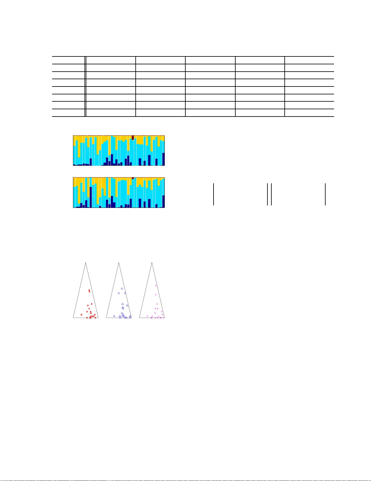
Dynamic Infinite Mixed-Mem b ership Sto c hastic Blo c kmo del Abstract Directional and pairwise measurements are often used to model inter-relationships in a so cial net work setting. The Mixed- Membership Sto c hastic Blo c kmo del (MMSB) was a seminal work in this a r ea, and many of its capabilities were extended s ince then. In this pap er, we propose the Dynamic Infi- nite Mixe d-Memb e rship sto chastic blo ckMo del (DIM3) , a generalis ed fr amework that ex- tends the existing w ork to a p otentially in- finite num b er of comm unities and mixture mem b erships fo r each of the net work’s no des. This mo del is in a dyna mic setting, where ad- ditional model parameters are in tro duced to reflect the degree of persistence b etw een one’s mem b erships at consecutive times. Accord- ingly , t wo effective p o sterior sampling str ate- gies and t heir results are presen ted using both synthetic and real data. 1 In tro duction Communit y learning is an emerging topic applicable to many so cial net working problems, and has recently attracted r esearch in teres t from the mac hine learn- ing co mmun ity . Many mo dels were prop osed in the last few years. Some notable earlier examples in- clude Sto chastic Blo ckMo del [16] and Infinite R ela- tional Mo del [13] wher e they aim to partition a net- work of no des into different groups ba sed on their pair- wise and directiona l binar y obser v a tio ns. T o address the phenomeno n that r elationships b etw een no des may change over times, the recent w or k in this area fo cuses o n the “dyna mic” settings. F or exam- ple, [23] used the sto chastic blo ckmodel to mo del the evolving comm unity’s behaviour ov er times. The work, how ever, assumes a fixed n umber of K communit ies exist where a no de i can p otentially belo ng to. How- ever, in man y applicatio ns, an accur ate g uess of K can be impractical. Infinite Relatio nal Mo del was incor p o rated [10] to ad- dress this pr oblem, where K can b e inferr ed from the data itself. Ho wev er, just as [13], its drawback is that the mo del assumes ea ch no de i must be lo ng to only a single communit y k (i.e., z i = k ). Therefore, a rela - tionship b etw een no des i and j can only b e deter mined from their comm unity indicator s z i and z j . This a p- proach can b e inflexible in ma ny scena rios, such as the monaster y example depicted in [1]. T o this end, the authors in [1] intro duced the concept of mixed- mem b ership, where they ass ume ea ch no de i may be- long to multiple communities. The mem b ership in- dicator is no lo ng er s ampled from each pa ir of com- m unity indicators z i and z j . Instead, they a re sam- pled from pair s o f in teractions b e t ween no des i and j . A few v ariants were s ubs equently prop osed fr o m MMSB, examples include: [5, 22] extends the mixture- mem b ership model with a dynamic setting; [15] ex- tends the MMSB in to the infinite case; and [14] incor- po rates the no de’s metadata infor mation into MMSB. In prac tice, the above discussed asp ects (infinite, dy- namic, mixture membership a nd data-driven infer- ence) are often embedded int o one complex netw or k environmen t, as se e n in the increa sing so cia l net- working activities. How ever, there is no work re- po rted o n a ddr essing all these a sp ects tow ards a flex- ible and genera lised framework. T o this end, we feel the emerg ent need to effectively unify these ab ov e men- tioned mo dels and to pr ovide a flex ible and genera lised framework which can encapsula te the adv antages from most of these w or ks. Accordingly , w e pro p ose the Dynamic Infinite Mixe d-Memb ership sto chastic blo ck- Mo del (D IM3) . DIM3 allows the following feature s. Firstly , it allows the infinite num b er of comm unities; secondly , it allows mixed-membership for each no de; thirdly , the mo del extends to the dynamic settings. Lastly , it is apparent that in ma ny so c ial netw ork ing applications, a node ’s member ship may b ecome p er- sistent over cons e c utive times, for example, a p erson’s opinion o f his p eer is mor e likely to b e cons is tent in t wo co nsecutive times. T o model p ers istence, we here dev is e t wo differe nt im- plement ations . The first is to hav e a s ing le mem b er- ship distribution for e ach no de at differ ent time in- terv a ls. The persis tence factor is dep endent on the statistics o f each no de’s int era ctions with the res t of the no des. The second implementation is to allow a set of mixed-membership distributions to asso ciate with each no de , and they are time-in v ariant. The num b er of e le men ts in the se t v a ries no n-p erimetrically similar to that of used in [2]. The per sistence factor is de- pendent o n the v alue of mem b ership indicator at the previous time. Two effective sampling algorithms ar e consequently designed for our pro p o sed mo dels, using either the Gibbs and Slice sampling technique for efficient mo del inference. The r est o f the article is or ganised in the following: Section 2 in tro duces our main fra mework a nd explains how it can incorp orate infinite communities in a dy- namic setting. The t wo mo dels are explained, and their infer e nc e sc hemes are also detailed in Sec tion 3 . In Section 4, we show the exp e rimental results of the several prop os e d mo dels using b oth the synthetic and real-world so cial netw or k data. Conclusions a nd future works can b e found in Section 5. 2 The DIM3 Mo del 2.1 Notations F or the notational clar ity , w e define all the symbols first, in which they will freq ue ntly app ear in v ario us sections in the rest of the pap er. W e us e E = { e t ij } 1: T n × n to denote the entire set of directiona l and binar y ob- serv ations: if i has a r elationship to no de j at time t , it implies e t ij = 1. Otherwise, e t ij = 0. Note that the di- rectional rela tio n e t ij discussed here is spe cific to each pair of communities membership indicators ( s t ij , r t ij ). F or each pair of no des , i and j , at time t , s t ij refers to the sender’s commun ity member ship indicator . Corre- sp ondingly , r t ij is for the receiver’s communit y mem- ber ship indica tor. F or the reaso n of s implicity and also making notations inline with what was used in the traditional HDP litera ture, we use Z to denote all the hidden lab els { s t ij , r t ij } . F or each no de i at time t , there is a mixed-membership distribution, π t i having infinite comp o ne nts, and the k th comp onent o f π t i , i.e., π t ik represents the “ signifi- cance” of communit y k for no de i . There is als o a role- c ompatibility matrix W used. As the num ber of co mm unities can beco me po tent ially in- finite, the dimension o f W can po tent ially b e ∞ × ∞ where its ( k , l ) th ent ry , i.e., W k,l represents co mpati- bilities b etw een communities k and l . Commonly , one assumes that each W k,l is i.i.d fr o m B eta ( λ 1 , λ 2 ) which gives conjuga cy to the Berno ulli distribution used to generate e t ij [14]. W e use n t k,l to deno te the num ber o f links from commu- nities k to l , i.e., the num be r of times in which s t ij = k and r t ij = l simultaneously . W e let n t k,l = n t, 1 k,l + n t, 0 k,l . n t, 1 k,l denotes the par t of n t k,l where the co rresp ond- ing e t ij = 1. The num b er of times that a no de i has participated in commun ity k (b oth as a se nding and receiving) at time t is repre sented b y N t ik . 2.2 Mixture Time V arian t (MTV) and Mixture Time Inv ariant (M TI) Mo dels T o address the phenomeno n that one’s so cial co m- m unity’s member ships may change over times, in o ur DIM3 mode l, w e allow each no de’s mixed- mem b ership indicators to change cross times. Additionally , it is im- per ative that these indicators should hav e some p er- sistence with its past v alues which reflects the rea lity of so cial b e haviour. The mo delling is achiev ed in tw o wa ys. The first is to allow the mixed-membership distributions itself to change over times. How ever, there is only a s ingle (but different) distribution for eac h no de at time t . The mem b ership indicator o f a no de at time t is dep endent on the “statistics” of a ll membership indicators of the same no de at t − 1 and t + 1. This is illustrated in the “Mixture Time V ariant (MTV)” version. The second method is to allow the mixed-membership distributions to stay inv ariant ov er times. How ever, there may be infinitely-po ssible many distributions as- so ciated with each no de, but due to a HDP prior, of- ten, o nly a few distributions will be discov ered. This is illustra ted in the “Mixture Time Inv aria nt (MTI)” mo del. In this cas e , the membership indicator at time t is dep endent and more likely to hav e the same v alue as it was in t − 1. In b oth cases, the p ersistence effect is a chiev ed through a stic ky parameter κ which is a dded to alter the mem- ber ship distributions. 2.3 Mixture Time V arian t (MTV) Mo del In Figure 1, w e show the gra phica l mo del of the MTV- DIM3 mo del. Here we only show all the v ariables in- volv ed for time t , and omit the other times, where the structure is identical. β γ π t i π t j s t ij r t ij e t ij α W n λ 1 λ 2 κ N t − 1 i · N t − 1 j · Figure 1: The MTV-DIM3 Mo del The corresp onding gene r ative pro cess is provided a s follows: 1. Global Setting - wher e its v alue is shar ed ac r oss all times 1 : T . • β ∼ GE M ( γ ) • W k,l ∼ B eta ( λ 1 , λ 2 ) ∀ k , l 2. Mixed-mem b ership distribution • π t i ∼ D P  α + κ, α β + κ 2 n · P k N t − 1 ik δ k α + κ  denotes a no de i ’s mixed-members hip distribution at time t . 3. Relationship Sa mpling • F or ea ch pair of i, j ∈ { 1 , · · · , n } , t ∈ { 1 , · · · , T } – s t ij ∼ M ul ti ( π t i ): sending communit y’s mem b ership indicator ; – r t ij ∼ M ul ti ( π t j ): receiving co mmun ity’s mem b ership indicator ; – e t ij ∼ B er noul l i ( W s t ij ,r t ij ) r elation from no des i to j at time t . Here N t − 1 ik = P N l =1 1 ( s t − 1 il = k ) + P N l =1 1 ( r t − 1 li = k ), representing the count num b er that a no de i has bee n asso ciated with a communit y k at time t − 1. β is used as a g lobal random v ariable, repres entin g the “significance” of all exis ting comm unities at all times, while W is the co mm unities’ compatibility ma- trix a s descr ib ed prev iously . As the prior P ( W ) is element-wise B eta distributed, which is c onjugate to the Bernoulli distribution P ( e t i,j | . ). Therefore, we can obtain a marginal distribution of P ( e t i,j ), i.e., R W p ( e t i,j | W ) p ( W ) d ( W ) analytically , and hence do no t need to explicitly sample v alues of W . The mixed-membership distribution { π t i } 1: T 1: n is sam- pled fro m the Dirichlet Pro ces s with a concen- tration par ameter ( α + κ ) and a base measure α β + κ 2 n P k N t − 1 ik δ k α + κ . There will b e N × T of these distri- butions. They jointly describ e each no de’s a ctivities. It should b e noted that each π t i is resp ons ible to gen- erate bo th the senders’ label { s t ij } n j =1 from node i and receivers’ lab el { r t j i } n j =1 to no de i . In the bas e measure, the intro duce d sticky pa rameter κ stands for each no de’s time influence on its mixe d- mem b ership distribution. In another words, w e as- sume that ea ch no de’s mixed-members hip distribution at time t will b e largely influenced by its ac tiv ities at time t − 1. This is r eflected in the hidden label’s multi- nomial distribution that the previous e x plicit activities will o ccupy a fixed prop ortio n κ α + κ to the current dis- tribution. The lar ger the v alue of κ , the mor e weight that the activities at t − 1 is g o ing to play at time t . As our metho d is la rgely based on the HDP framework, therefore, w e will use the popular “Chinese Restau- rant F ranchise (CRF)” [20, 2] analog y to further ex- plain our mo del. Using the CRF analogy , the mixed- mem b ership distribution asso cia ted with a no de i at time t can b e seen a s a restaurant π t i , with its dishes representing the co mm unities. If a cus tomer s t ij (or r t j i ) eats the dish k at the i th restaura nt at time t , then s t ij ( r t j i ) = k . ∀ t > 1, the restaura nt π t i would have its own sp ecials on the served dishes, repr esenting the “sticky” co nfiguration in the gra phical mo del. Con- trast to the sticky HDP-HMM [2] approa ch, which places sp ecia l on one dish only , in our work, we allow m ultiple sp ecials, wher e the weight of each sp ecia l dish is adjusted accor ding to the num b er of served dishes at this r estaurant at time t − 1 , i.e., κ 2 n P k N t − 1 ik δ k . Therefore, w e can ensure tha t the s pe cial dishes ar e served p er sistently across times in the same res ta u- rant. 2.4 Mixture Time In v arian t (M TI) Mo del W e s how the MTI-DIM3 mo del in Figure 2. In this model, e ach no de has a v ariable num ber of mem b ership distributions ass o ciated with it, which may p otentially b e infinite. A t ea ch time t , its mem- ber ship indicator s t ij is generated from π s t − 1 ij . In order to encourag e p ersistence, ea ch π ik was genera ted from a corresp onding β , where κ was added to β ’s k th com- po nent [2, 3, 4]. The corr e sp onding g enerative pro cess of the MTI- DIM3 mode l is provided as follows: β γ π ( k ) i ∞ π ( l ) j ∞ s t ij r t ij e t ij κ W λ 1 λ 2 α i α j s t − 1 ij r t − 1 ij s t +1 ij r t +1 ij Figure 2: The MTI-DIM3 Model 1. Global Setting - wher e its v alue is shar ed ac r oss all times 1 : T . • β ∼ GE M ( γ ) • W k,l ∼ B eta ( λ 1 , λ 2 ) , ∀ k , l 2. Mixed-mem b ership distribution • π ( k ) i ∼ D P  α i + κ, α i β + κ δ k α i + κ  denotes a no de i ’s mixed-membership distribution. 3. Relationship Sa mpling • F or ea ch pair of i, j ∈ { 1 , · · · , n } , t ∈ { 1 , · · · , T } – s t ij ∼ M ul ti ( π ( s t − 1 ij ) i ): sending c o mmu - nit y’s membership indicator; – r t ij ∼ M ul ti ( π ( r t − 1 ij ) j ): receiving commu- nit y’s membership indicator; – e t ij ∼ B er noul l i ( W s t ij ,r t ij ) r elation from no des i to j at time t . β and W ’s g eneration is the same a s in Section 2.3. The se t of mem b ership indicators { s t ij , r t j i | j = 1 , · · · , n, t = 1 , · · · , T } will b e sampled from the time-inv a riant mixed-mem b ership distribution set, { π ( k ) i } ∞ k =1 , wher e each member is indep endently dis- tributed fro m a Dirichlet Pr o cess with a concentration parameter ( α + κ ) and a bas e meas ure α β + κ δ k α + κ . A t time t , a mem b ership indicator s t ij (or r t j i ) is sam- pled from the distribution π ( s t − 1 ij ) i (or π ( r t − 1 ji ) i ) ∀ i ∈ { 1 , · · · , n } . Back to the C RF [20] analo gy , we have N × ∞ ma - trix, where its ( i, k ) th element refers to π ( k ) i , which can be seen as the weight s of ea ting each of the av ail- able dishes. A customer s t ij (or r t j i ) therefor e can only trav el be tw een restaur a nts lo cated at the i th row of the matrix. When π ( k ) i ’s k th comp onent is more likely to be large r , it mea ns that the dish k is a sp ecial dish for restaura nt k . Therefore, a custo mer is at restaurant k at time t − 1, is more likely to eat the same dish ( i.e., k th dish), and hence to stay at re staurant k a t time t . 3 Inference Two sampling s chemes ar e implemented to complete the infer e nce on MTV-DIM3 : the sta ndard Gibbs sampling a nd Slice-Efficient sampling, which b oth tar- get the po sterior distributio n. Due to the spa ce limit, we do not present her e the detailed sampling s cheme of the MTI-DIM3 . Interesting readers can refer to the supplement ar y materia l . Due to the double-blind re- view po licy , we ano nymously put the supplementary material in 1 3.1 Gibbs Sampli ng The Gibbs Sa mpling scheme is large ly ba s ed on [20]). The v a riables of interest are : β , Z and a uxiliary v ar i- ables ˆ m , where ˆ m refers to the n umber of tables eating dish k a s used in [20 , 2] without coun ting the tables that generated from the sticky po rtion, i.e., κN t − 1 ik . Note that we do not sa mple { π t i } 1: T 1: n , as it gets in te- grated out. Sampling β β is the prio r for all { π t i } s , which can be thought as the ratios betw een the communit y comp onents for all co mmunities. Its p osterior distr ibutio n is obtained through the auxiliar y v ariable ˆ m : ( β 1 , · · · , β K , β µ ) ∼ D i r ( ˆ m · 1 , · · · , ˆ m · K , γ ) (1) where its detail ca n b e found in [20 ]. Sampling { s t ij } 1: T n × n , { r t ij } 1: T n × n Each observ ation e t ij is sampled from a fixed Bernoulli distribution, where the Bernoulli’s pa- rameter is contained within the r ole-compatibility matrix W indexed (row a nd column) b y a pair of corr esp onding members hip indicators { s t ij , r t ij } . W.o.l.g, ∀ k , l ∈ { 1 , · · · , K + 1 } , the join t pos terior probability of ( s t ij = k , r t ij = l ) is: 1 Here is the anonymous link address. P ( s t ij = k , r t ij = l | Z \{ s t ij , r t ij } , e , β , α, λ 1 , λ 2 , κ ) ∝ P ( s t ij = k |{ s t ij 0 } j 0 6 = j , { r t j 0 i } n j 0 =1 , β , α, κ, N t − 1 i ) · 2 n Y l =1 P ( z t +1 il | z t i · /s t ij , s t ij = k , β , α, κ, N t +1 i ) · P ( r t ij = l |{ r t i 0 j } i 0 6 = i , { s j i 0 } n i 0 =1 , β , α, κ, N t − 1 j ) · 2 n Y l =1 P ( z t +1 j l | z t j · /r t ij , r t ij = l , β , α, κ, N t +1 j ) · P ( e t ij | E \{ e t ij } , s t ij = k , r t ij = l , Z \{ s t ij , r t ij } , λ 1 , λ 2 ) (2) Detailed deriv ations of Eq. (2) is found a t the supplement ar y materials. Assuming the current sample o f { s t ij , r t ij } having v alues rang ing b etw een 1 . . . K , we let undiscov- ered (new) communit y to b e indexed by K + 1. Then, to sample a pair ( s t ij , r t ij ) in questio n, w e need to c alculate all ( K + 1) 2 combinations o f v al- ues for the pair . Sampling ˆ m Using the res taurant-table-dish analogy , we de- note m t ik as the num ber of tables eating dish k ∀ i, k , t . This is related to the v ar iable ˆ m used in sampling β , but a lso including the count s of the “un-sticky” p ortion, i.e., α β k . The sampling of m t ik is to inco rp orate a similar strategy as [20, 2], which is indep endently dis- tributed from: Pr( m t ik = m | α, β k , N t − 1 ik , κ ) ∝ S ( N t ik , m )( α β k + κN t − 1 ik ) m (3) Here S ( · , · ) is the Stirling num ber o f first kind. F or ea ch no de, the ratio of genera ting new tables can result fro m t wo factors: (1) Dirichlet prio r with para meter { α, β } and (2) the sticky config- uration fr o m member ship indicator s at t − 1 , i.e ., κN t − 1 ik . T o sa mple β , we need to only include ta bles g ener- ated from the “un-sticky” po r tion, i.e., ˆ m , where each ˆ m t ik can b e obtained from a single Bino mial draw: ˆ m t ik ∼ B inomi a l ( m t ik , α β k κ 2 n N t − 1 ik + α β k ) . (4) 3.2 Ada pted Sl ice-Efficient Sampli ng W e also inco rp orate the slice-efficie nt sampling [12][21] to our mo del. The original sampling s cheme was de- signed to sample the Dirichlet Pro cess Mixtur e mo del. In order to adapt it to our framework, which is ba sed on a HDP prio r and als o has pa ir-wise membership in- dicators, we use auxiliary v ariables U = { u t ij,s , u t ij,r } for each of the la tent mem b ership pair { s t ij , r t ij } . Hav- ing the U s, we are able to limit the n umber o f com- po nents in which π i needs to b e co nsidered, w hich is infinite otherwise. Under the slice-efficient sampling f ra mework, the v aria ble s of in terest are now extended to: π t i , { u t ij,r , u t ij,s } , { s t ij , r t ij } , β , m : Sampling π F or each no de i = 1 , · · · , N : we generate π ′ t i us- ing s ticky-breaking pro cess [11], where each k th comp onent is gener ated using: π ′ t ik ∼ b eta( π ′ t ik ; a t ik , b t ik ), where a t ik = α β k + N t ik + κN t − 1 ik b t ik = α (1 − k X l =1 β l ) + N t i,k 0 >k + κN t − 1 i,k 0 >k (5) Here π k = π ′ k Q k − 1 i =1 (1 − π ′ i ). Sampling u t ij,s , u t ij,r , s t ij , r t ij W e use u t ij,s ∼ U (0 , π t is t ij ), u t ij,r ∼ U (0 , π t j r t ij ). Then the obtained hidden lab el is indep endently sampled from the finite ca ndida tes: P ( s t ij = k , r t ij = l | Z, e t ij , β , α, κ, N , π , u t ij,s , u t ij,r )) ∝ 1 ( k : π t ik > u t ij,s ) · 1 ( l : π t j l > u t ij,r ) · 2 n Y l =1 P ( z t +1 il | z t i · /s t ij , s t ij = k , β , α, κ, N t +1 i ) · 2 n Y l =1 P ( z t +1 j l | z t j · /r t ij , r t ij = l , β , α, κ, N t +1 j ) · P ( e t ij | E \{ e t ij } , s t ij = k , r t ij = l , Z \{ s t ij , r t ij } , λ 1 , λ 2 ) (6) Sampling β , m This is the same as the Gibbs s a mpling. The deriv atio ns of the ab ove equations can be re fer- enced to the Supplementary Mater ia ls. 3.3 Hyper-parameter Sampli ng The hyper-par ameters in volved are γ , α, κ . How ever, it is imp os s ible to compute their po sterior individually . Therefore, we place thr ee prio r distributions on some “combination” o f the v ar iables: A v ague ga mma prior G (1 , 1 ) is placed o n b oth γ , ( α + κ ). A b eta prior is placed on the ra tio κ α + κ . T o sample γ v alue, since log( γ )’s p oster ior distributio n is log-co ncav e, we use the Adaptive Rejection Sam- pling (ARS) metho d [19]. T o sample ( α + κ ), we use the Auxiliary V ariable Sam- pling [20] using the auxilia ry v a riable m in E q. (3) as prop osed in [20]. T o sample κ α + κ , we place a v ague b eta prior B (1 , 1) on it, with a likelihoo d of { m t ik − ˆ m t ik , ∀ i, k , t > 1 } in Eq. (4 ), the p osterio r is in an analy tical a nd sa mpla ble form, thanks to its conjuga te pr op erty . 3.4 Discussions Both the Gibbs Sampling and Slice-Efficient Sampling are tw o feasible wa ys of accomplishing o ur task. They hav e different pr os and cons. As mentioned pre v iously , Gibbs Sa mpling in our DIM3 integrates out the mixed-membership distr ibu- tion { π t i } . It is the “margina l appr oach” [1 7]. The prop erty of communit y exchangeabilit y makes it s im- ple to implement. How ever, theor etically , the obtained samples mix slowly as the sampling of e ach lab el is de- pendent on other lab els. The Slice-E fficient Sampling is one “conditional ap- proach” [12] while the members hip indicators are in- depe ndently sampled fro m { π t i } . In e a ch iteration, given { π t i } , we ca n pa rallelize the pro ces s of sampling mem b ership indicators, which may help to improv e the computation, esp ecially when the num ber of nodes , i.e., N b ecomes lar ger, and the num b er of co mm uni- ties, i.e., k b ecomes smaller . 4 Exp erimen ts The p erformance of the DIM3 mo del is v alida ted by exp eriments on synthetic datasets a nd s everal r eal- world da tasets. W e implement the o ur mo del’s finite- communities cas e as a ba seline algo rithm, namely as f-MTV and f-MTI . 4.1 Syn thetic Dataset F or the synthetic data generation, the v ariables ar e generated following [9 ]. W e use N = 2 0 , T = 3, and hence E is a 2 0 × 20 × 3 asymmetric and binary matrix. The parameter s are set up such that the 20 no des are equally partitioned int o 4 groups. The gr ound-truth of the mixed- mem b ership distribution for ea ch of the gr oups are: [0 . 8 , 0 . 2 , 0 ; 0 , 0 . 8 , 0 . 2; 0 . 1 , 0 . 05 , 0 . 85; 0 . 4 , 0 . 4 , 0 . 2]. W e co ns ider 4 different case s to fully assess DIM3 against the ground-truth, a ll lie in the 3- role compat- ibilit y ma trix. Case 1 : large dia g onal v alues and small non-diago nal v alues Case 2 : large dia gonal v alues and mediate non- diagonal v alues Case 3 : large no n- diagonal v alues and small diago nal v alues Case 4 : small diago nal v alues and mediate non- diagonal v alues The detailed v alue of the role- c ompatibility matrix on these four cases are shown in Fig ure 3. 4.1.1 MCMC Analysis The convergence behavior is tested in terms of t wo quantities: the cluster n umber K , i.e., the num ber of different v alues Z can take, and the estimated densit y D [12, 17], which is defined as: D = − 2 X i,j,t log   X k,l N t ik · N t j l 4 n 2 T p ( e t ij | Z, λ 1 , λ 2 )   (7) In our MCMC stationary analysis, we ran 5 indep en- dent Marko v ch ains and disca rded the first half of the Marko v chains a s a burn-in. With the ra ndom parti- tion of 3 initial classes as the starting p oint, 13 0 , 0 00 iterations are conducted in o ur s amplings. The simulated chains satisfy standard conv erge nc e cri- teria, as we implemen ted the test by using COD A pack age [18]. In Gelman a nd Rubin’s diagnos tics [6], the v alue of Prop ortiona l Sca le Reduction F acto r (PSRF) is 1.09 (with upp e r C.I. 1.27) for k, 1 .03 (with upper C.I. 1.09) for D in the Gibbs sa mpling, a nd 1.02 (with upper C.I. 1.06 ) for k, 1.02 (with upp er C.I. 1.02) for D in Slice sampling. The Geweke’s conv er- gence diagnos tics [7] is also employ ed, with propo rtion of firs t 10% a nd la st 5 0 % of the chain as compari- son. The corr esp onding z-sco res are a ll in the interv al [ − 2 . 09 , 0 . 85 ] for 5 chains. In addition, the stationarity and half-width tests of Heidelb erg and W elch Diagnos- tic [8] were b oth pas s ed in all the cases, with p -v a lue higher than 0.0 5. Based on all these statistics, the Marko v chain’s stationar y ca n be safely ensured in o ur case. The efficiency of the algorithms can be measured b y estimating the int egr ated a uto corre lation time τ for 0.95 0.05 0 0.05 0.95 0.0 5 0.05 0 0.95 0.95 0.2 0 0.05 0.95 0.0 5 0.2 0 0.95 0.05 0 .9 5 0 0.05 0 .0 5 0.95 0.95 0 0.05 0.05 0.95 0 0.2 0.05 0.9 5 0.95 0 0.2 Figure 3 : F our Cases of the Compa tibilit y Ma tr ix. (Cases 1- 4 as fro m left to right.) K and D . τ is a go o d per formance indicator as it measures the s tatistical error of Monte Carlo approx- imation o n a tar get function f . The smaller τ , the more efficient of the algo rithm. [12] used an estimator b τ as: b τ = 1 2 + C − 1 X l =1 b ρ l (8) Here b ρ l is the estimated a uto corre la tion a t la g l and C is a cut-off p oint, which is defined as C := min { l : | b ρ l | < 2 / √ M } , and M is the num ber of iterations. W e test the sa mpling efficiency of MTV-g and MTV-s on Case 1 with the same setting as [17]. Amo ng the whole 130 , 000 iter a tions, the first 30 , 00 0 samples are discarded a s a bur n-in a nd the rest is thinned 1 / 20. W e manually try different v alues of the hyper-par ameters γ and α and show the integrated auto corr e lation time estimator in T able 1. Although some outliers exist, w e can see that there is a general tre nd that, with fixed α v alue, the a uto correla tion function will decr ease when the γ v alue increa ses. This same phenomenon hap- pens on α while γ fixed. This fact meets our empir- ical knowledge. The larg er v alue of γ , α will help to discov er more clusters, then comes a s maller auto c o r- relation function. On the o ther hand, we admit that MTV-g and MTV-s do not show muc h difference in the Marko v chain’s mixing r ate as shown in T able 1. As mentioned in the pr e vious se ction, Slice sampling provides an mixed-membership distribution independent sampling scheme, which can enjoy the time e fficie nc y o f parallel computing in o ne iteration. F or large scale datasets, it is a n feas ible solutio n. While in Gibbs sampling, the para llel computing is imp ossible as the sampling v ar iables a re in a dep endent sequence. 4.1.2 F urther Performanc e W e will compar e the mo dels in terms of the Log- likelihoo d (in Figure 4); the av erag e l 2 distance be- t ween the mixed-membership distributio ns and its ground-truth; and the one be tw een the p oster ior role- compatibility matrix and its g round-truth (in T able 2). F ro m the log-likeliho o d comparison in Figure 4 , we can see that the MTI mo del perfo r ms b etter than the MTV mo del. On the average l 2 distance to the −450 −400 −350 −300 −250 −200 −150 −100 −50 0 f−MTV MTV−g MTV−s f−MTI MTI Case 1 the Log−likelihood −350 −300 −250 −200 −150 −100 f−MTV MTV−g MTV−s f−MTI MTI Case 2 −400 −350 −300 −250 −200 −150 −100 −50 f−MTV MTV−g MTV−s f−MTI MTI Case 3 −300 −250 −200 −150 −100 −50 f−MTV MTV−g MTV−s f−MTI MTI Case 4 Figure 4: Log-likelihoo d Performance T a ble 3: Running Time (Seconds p er iteratio n) N. f-MTV MTV-g MTV-s f-MTI MTI 20 0 . 20 0 . 28 0 . 23 0 . 15 0 . 31 50 1 . 03 1 . 52 1 . 29 0 . 95 1 . 91 100 3 . 69 5 . 76 4 . 81 3 . 74 7 . 49 200 15 . 61 24 . 17 19 . 87 15 . 82 30 . 1 9 500 106 . 96 154 . 45 119 . 82 105 . 61 20 2 . 09 1000 49 3 . 44 888 . 86 642 . 28 597 . 29 11 0 2 . 90 ground-truth pe rformance, the MTI mo del also p er- forms b etter. Here we co mpare the co mputational complexity (Run- ning Time) of the mo dels in one iteration, with K discov ered co mmu nities and show the r e sults in T a- ble 5. W e dis cuss MTV-g and MTV-s as a n ins tance. In MTV-g , the num b er of v ar ia bles to b e sa mpled is (2 K + 2 n 2 T ) , while a total of (2 K + 4 n 2 T + nT ) v a ri- ables are sampled in MTV-s . How ever, the po sterior calculation o f Z in MTV-s ca n b e directly obtained from the members hip distribution, while we need to calculate the ra tio for each of Z in MTV-g . Also, the U v alue at each time can b e sampled in one op eratio n as its indep endency in MTV-s . Th us, the result of MTV-s runs faster than MTV-g is in accor da nce with our assumption. 4.2 Real W orld Dataset P erformance W e ra ndomly selected 7 rea l world datasets for be nch- mark testing. Their de ta iled information, including the num b er o f no des, the num b er of edges, edge types and time interv als , are g ive in T able 4 . W e will discuss T a ble 1: Integrated Autoco rrelatio n Times Estimator b τ for K a nd D K D Sampling ❍ ❍ ❍ ❍ ❍ γ α 0.1 0.3 0.5 1 2 0.1 0.3 0.5 1 2 MTV-g 0.1 177.2 93.65 26 .91 50.21 11.24 3 5 8.8 148.3 2 3 .94 8 4.75 4.31 0.3 260.5 54.00 9.18 5.31 6.56 389 .5 315.0 3.11 26.32 4.78 0.5 1 .83 8.3 3 7.54 3.95 5.24 2.88 79.34 90 .93 3.17 3.82 1.0 5 .57 6.4 5 3.44 3.64 4.56 3.19 2 .7 8 1.76 8 .14 5.7 4 2.0 4 .30 2.8 7 3.35 2.98 3.28 95 .4 8 1.91 3.29 8.74 6.5 5 MTV-s 0.1 248.6 90.63 16 1.3 9.58 17.69 8.67 59.90 57 .57 1.87 3.70 0.3 120.6 66.23 44 .35 11.40 7.28 29.05 20 .64 30.01 45.5 7 3.4 0 0.5 18.99 27.27 6.08 8.76 10.40 39.66 3.8 7 5 .30 3.1 7 5.8 3 1.0 5 .79 9.1 9 11.85 8.46 7.2 5 40 .51 4.85 3.12 6.88 10.51 2.0 3 .17 8.4 1 5.35 5.48 5.05 25 .5 4 34.82 4.61 35.61 12 .68 T a ble 2: Average l 2 Distance to the Ground-tr uth Cases Role-Compatibility Matrix Mixed-Memberships f-MTV MTV-g MTV-s f-MTI MTI f-MTV MTV-g MTV-s f-MTI MT I 1 0 . 529 0 . 625 0 . 848 0 . 114 0 . 086 0 . 366 0 . 384 0 . 403 0 . 199 0 . 19 1 2 0 . 439 0 . 225 0 . 339 0 . 195 0 . 204 0 . 355 0 . 355 0 . 319 0 . 207 0 . 2 27 3 0 . 134 0 . 201 0 . 513 0 . 117 0 . 087 0 . 278 0 . 289 0 . 589 0 . 208 0 . 18 7 4 0 . 195 0 . 2 14 0 . 267 0 . 2 20 0 . 219 0 . 258 0 . 285 0 . 2 77 0 . 192 0 . 182 more on the first tw o datasets in the following. 4.2.1 Log-lik eliho o d Performanc e on V arious Real W orld Datasets T a ble 4: Data Set Information Dataset No des Edge Time T yp e Kapferer 3 9 256 2 friends Sampson 18 168 3 like Stu-net 50 351 3 friends Enron 41 1980 12 email Newcom b 17 1020 15 contact F re e man 32 357 2 friends Coleman 73 506 2 co-work Since no unambiguous gro und- tr uth can b e found in the real w orld datas e t, we mainly use lo g-likelihoo d to verify the corres p o nding mo del’s p erfor mance: The larger the log-likelihoo d, the b etter appropr ia teness of the mo del to data. T a ble 5 shows the 9 5% confidence interv al in test data log-likeliho o d o f our mo dels v ers us the clas s ical ones. The black b old type deno tes the larg est v alue in each o f the rows. W e ca n se e the MTI mo del usually p erforms better , while the MTV model may be bo ther ed b y the ov er-fitting pr oblem in our assumption. 4.2.2 Kapferer T ailor Shop The Kapferer T ailor Shop data [16] records int era c- tions in a tailor sho p a t tw o time p oints. In this time per io d, the employees in the shop a re negotia ting for higher wages. The data s e t is of pa rticular int eres ting as t wo strikes ha ppen after each time p oint, w ith the first fails and the second succeeds . W e mainly use the “work-assis ta nce” interaction ma - trix in the datas et. The employ ees hav e 8 o ccupations: head ta ilor (19), cutter (16), line 1 tailor (1 -3, 5-7 , 9, 11-14 , 21, 24), button machiner (25-2 6), line 3 tailor (8, 15, 2 0, 22-23 , 27-2 8), Irone r (2 9, 33, 39), cotton boy (30-32 , 34- 3 8) and line 2 tailo r (4, 10, 17-18 ). W e ca n s ee the y ellow ba r at time point 2 are larger than the ones at time p o int 1, whic h means p eople tending to have another gr oup at time p oint 2, rather than mos tly dominated b y one large gr oups at time po int 1. 4.3 Sampson Monastery Dataset The Sampso n Monastery da taset are us ed here to do an explor atory study . There are 1 8 monks in this dataset, and their soc ia l link age data is collected a t 3 different time p oints with v arious relations . Here we esp ecially fo cus on the like-sp ecification. In the lik e- sp ecification data, each monk selects thr e e monks as his to p-closed friends. In our settings , we mark the se- T a ble 5: Log -likelihoo d Performance (95% Confidence Interv al = Mean ∓ 1 . 9 6 ∗ Standard E rror ) Dataset f-MTV MTV-g MTV-s f-MTI MTI Kapferer − 24 7 . 4 ∓ 28 . 9 − 267 . 7 ∓ 3 6 . 3 − 332 . 6 ∓ 51 . 3 − 43 . 4 ∓ 0 . 5 − 88 . 9 ∓ 4 . 4 Sampson − 290 . 0 ∓ 5 9 . 4 − 219 . 2 ∓ 8 . 4 − 2 5 6 . 4 ∓ 1 1 . 1 − 79 . 3 ∓ 5 . 9 − 53 . 3 ∓ 4 . 1 Stu-net − 574 . 5 ∓ 18 . 4 − 505 . 8 ∓ 32 . 1 − 506 . 3 ∓ 21 . 2 − 42 . 3 ∓ 18 . 0 − 47 . 2 ∓ 7 . 1 Enron − 2398 . 3 ∓ 7 5 . 4 − 270 1 . 4 ∓ 51 . 3 − 2489 . 9 ∓ 55 . 4 − 656 . 8 ∓ 56 . 4 − 1 368 . 3 ∓ 2 3 . 1 Newcom b − 1342 . 7 ∓ 32 . 1 − 1 294 . 1 ∓ 4 1 . 7 − 1 320 . 6 ∓ 32 . 9 − 44 4 . 0 ∓ 26 . 3 − 343 . 4 ∓ 3 4 . 5 F re e man − 378 . 9 ∓ 28 . 6 − 406 . 8 ∓ 37 . 8 − 406 . 9 ∓ 49 . 5 − 22 . 5 ∓ 3 . 1 − 2 7 . 2 ∓ 9 . 2 Coleman − 1321 . 8 ∓ 116 . 7 − 1 270 . 2 ∓ 101 . 1 − 1283 . 9 ∓ 1 68 . 3 − 54 . 8 ∓ 39 . 3 − 41 . 9 ∓ 1 . 0 5 10 15 20 25 30 35 0 0.2 0.4 0.6 0.8 1 5 10 15 20 25 30 35 0 0.2 0.4 0.6 0.8 1 Figure 5: MTI Performance on Sampson Mona stery Dataset (T op: Time 1; Bottom: Time 2.) 1 2 3 4 5 6 7 8 9 10 11 12 13 14 15 16 17 18 A B C 1 2 3 4 5 6 7 8 9 10 11 12 13 14 15 16 17 18 A B C 1 2 3 4 5 6 7 8 9 10 11 12 13 14 15 16 17 18 A B C Figure 6: MTI Performance on Sampson Mona stery Dataset (from Left to Right: Time 1-3.) lected r elations as 1 , o therwise 0 . Thus, an 18 × 18 × 3 so cial netw or ks data set is co nstructed, with ea ch row has three elements v alued 1. According to the previo us studies [14, 2 2], the monks are divided into 4 communities: Y oung T u rks , L oyal Opp osition , Outc asts and a n interstitial group. Figure 6 shows the deta ile d res ults of MTI . As thr ee communities hav e been detected, we put all the results in a 2-simplex, with which we deno te as A , B a nd C . As we can see, most of the monks stay the in the same area during the 3 time p o ints, except for the monk 8 and 9. W e also provide the ro le-compatibility matrix in Fig- ure 7 for co mparison. Co mpared to the result in [22], our results a re with a lar ger co mpatibilit y v alue within the same role. Also, the first ro le’s v a lue in o ur mo del is 0 while it is ab out 0.6 in [2 2]. 0.09 0 0.0 0.05 0 .9 9 0.02 0.01 0 0.96 0.01 0 0.0 3 0.02 0.78 0 0.02 0 0.6 7 Figure 7: Role Compatibility Matrix (Left: MTV-g ; Right: MTI ) 5 Conclusion & F uture W ork In this pap er, we have extended the exis ted mixed- mem b ership sto chastic blo ckmodel to the infinite com- m unity case in the dyna mic setting. By incorp or a ting the mix e d-membership dis tribution-sticky paradigm, we have rea lized the time-co rrelation description on the hidden lab el. Both the Gibbs sampling a nd adapted Slice-E fficient sampling hav e b een utilized to achiev e the inference target. Quantit y analysis on the MCMC’s conv ergence behaviour, including the conv ergence test, auto cor r elation function, etc., have bee n provided to further enhance the inference per for- mance. The r esults in the exp er iment s verify that our DIM3 is effective to re-cons truct the dy na mic mixed- mem b ership distribution and the role- c o mpatibility matrix. Some future work includes a systematic application of DIM3 to v arious la rge real- world so cia l netw orks. In particular , we a re also interested in adapting our mo del to many a typical applications, for example, where sequences of netw orks hav e non-binary and di- rectional mea surements. W e will a ls o study other more flexible framework for mo delling p ersis tence of mem- ber ships over times. Lastly , we w ill p erfor m an exten- sive study into patterns of joint dyna mics of { π t i } and to extract meaningful latent infor mation fro m them. This is do ne in a setting where the num ber o f co mp o- nent s b etw een π t 1 i and π t 2 i may differ. References [1] E.M. Airoldi, D.M. Blei, S.E . Fienberg, and E.P . Xing. Mixed mem b ership sto chastic blo ckmod- els. The Journal of Machine L e arning R ese ar ch , 9:1981 –201 4, 20 08. [2] E.B. F ox, E.B. Sudderth, M.I. J ordan, a nd A.S. Willsky . An hdp-hmm for systems with state pe r - sistence. In Pr o c e e dings of t he 25th international c onfer enc e on Machi ne le arning , pages 31 2–319 . A CM, 200 8 . [3] Emily F ox, Erik B Sudderth, Michael I Jordan, and Alan S Willsk y . Bay esian nonpa rametric in- ference of switching dynamic linear mo dels. Signal Pr o c essing, IEEE T r ansactions on , 59(4):156 9– 1585, 2 011. [4] Emily B F ox, Erik B Sudderth, Mic hael I Jordan, and Alan S Willsky . A sticky hdp-hmm with ap- plication to spe a ker diarization. The Annals of Applie d St at ist ics , 5 (2A):1020 – 1056 , 201 1. [5] W. F u, L. Song , and E.P . Xing. Dynamic mixed mem b ership blo ckmodel for evolving netw or ks. In Pr o c e e dings of the 26th Annual International Confer enc e on Machine L e arning , pages 329–3 3 6. A CM, 200 9 . [6] A. Gelman and D.B. Rubin. Inference from iter - ative simulation us ing mult iple sequences. Statis- tic al scienc e , 7(4):45 7 –472 , 1 992. [7] J. Geweke. Ev aluating the acc uracy of sa mpling- based a pproaches to the calculation of p oster ior moments. In Bayesian S tatistics , pages 1 69–1 93. Univ er s it y Press, 1992 . [8] Philip Heidelb erg er and Peter D. W elch. A sp ec- tral metho d for c onfidence interv al generation and r un length control in s imulations. Commun. ACM , 24 (4):233– 245, April 1981. [9] Qirong Ho, Le Song, and E ric P . Xing. Evolving cluster mixed-membership blo ckmodel for time- evolving net works. Journal of Machi ne L e arning R ese ar ch - Pr o c e e dings T r ack , 15:34 2–35 0, 20 11. [10] Katsuhiko Ishig uro, T omoha ru Iwata, Naonori Ueda, a nd Joshua B. T enenbaum. Dynamic in- finite r e la tional mo del for time-v arying relationa l data analysis. In NIPS , pages 9 1 9–92 7. Curra n Asso ciates, Inc., 2010 . [11] Hemant Ishw ar an and La ncelot F. James. Gibbs sampling methods for s tick-breaking prior s. Jour- nal of the Americ an Statistic al Asso ciation , 96:161 –173 , 200 1. [12] Maria Kalli, Jim E. Griffin, and Stephen G. W alker. Slice sampling mixture mo dels. St atis- tics and Computing , 21(1):93– 105, January 2011 . [13] C. Kemp, J.B. T ene nbaum, T.L. Griffiths, T. Y a- mada, and N. Ueda. Learning systems o f con- cepts with an infinite relational mo del. In Pr o- c e e dings of the national c onfer enc e on artificial intel ligenc e , volume 21 , pa ge 3 81. Menlo Park, CA; Ca mbridge, MA; London; AAAI Pr ess; MIT Press; 1999 , 200 6. [14] D.I. Kim, M. Hughes, and E. Sudderth. The non- parametric metadata dep endent relationa l mo del. In Pr o c e e dings of the 29th Annual International Confer enc e on Machine L e arning . A CM, 2012 . [15] P .S. K outsourela kis a nd T. Elia ssi-Rad. Finding mixed-memberships in so cial netw or k s. In Pr o- c e e dings of the 2008 AA AI spring symp osium on so cial information pr o c essing , 2 008. [16] K. Nowicki and T.A.B. Snijders. Estimation and prediction for sto chastic blo ckstructures. Journal of the Americ an Statistic al Asso ciation , 96(455 ):1077– 1087, 200 1. [17] O. Papaspiliop oulo s a nd G.O. Rober ts. Retr o- sp ective marko v chain monte ca rlo metho ds for dirichlet pr o cess hier archical mo dels. Biometrika , 95(1):169 –186 , 200 8. [18] Martyn P lummer , Nicky Best, K ate Cowles, and Karen Vines. Co da: Conv ergence dia gnosis and output a nalysis for mcmc. R News , 6(1):7–11, 2006. [19] Carl Edw ar d Rasmussen. The infinite gaussian mixture mo del. A dvanc es in n eur al information pr o c essing systems , 12(5 .2):2, 20 00. [20] Y.W. T eh, M.I. Jor dan, M.J. Bea l, and D.M. Blei. Hierarchical dirich let pro cesses . Journ al of the Americ an Statistic al Asso ciation , 10 1(476):1 566– 1581, 2 006. [21] S.G. W alker. Sampling the dir ichlet mixture mo del with slices. Communic ations in Statis- ticsSimulation and Computation R  , 36 (1 ):45–54 , 2007. [22] E.P . Xing, W. F u, and L. So ng. A state-space mixed mem b ership blo ckmodel for dynamic net- work tomog raphy . The Annals of Applie d Statis- tics , 4(2):535 –566 , 2 010. [23] Tianbao Y ang , Y un Chi, Shenghuo Zhu, Yihong Gong, and Ro ng Jin. Detecting communities and their evolutions in dynamic so cia l netw orks - a bay esian approa ch. Machine Le arning , 82(2):15 7– 189, 2011.