A Greedy Approximation of Bayesian Reinforcement Learning with Probably Optimistic Transition Model

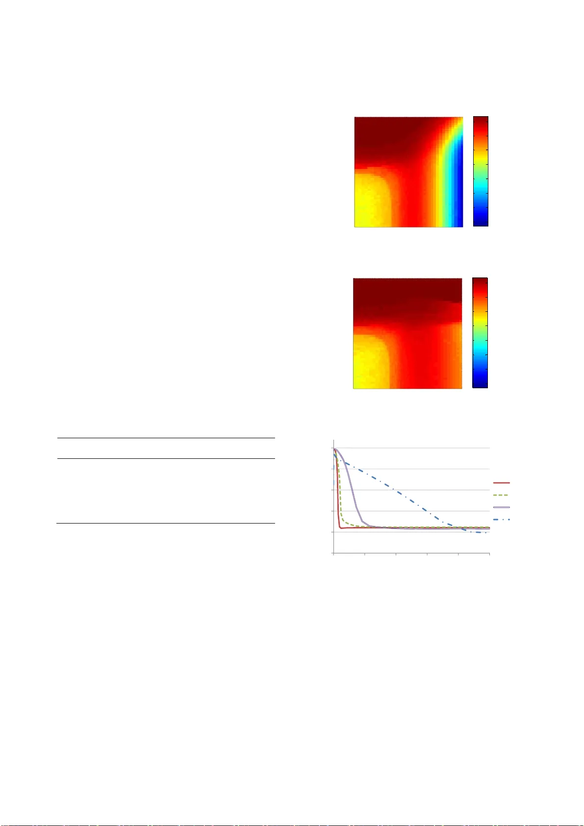
A Greedy Approximation of Bayesian Reinforcement Learning with Probably Optimistic Transition Model Kenji Kawaguchi BWBP Artificial Intelligence Laboratory Tokyo, Ja pan kawaguchi.kenji9@gmail.com Mauricio Araya-López Nancy Unive rsité / INRI A Nancy, Fr ance mauricio.araya@inria.fr ABSTRACT Bayesian Reinforcement Learning (RL) is capable of not only incorporating domain knowledge, but also solving the exploration- exploitation dilemma in a natur al way. As Bayesian RL is intrac- table except for special cases, previous work has proposed several approximation methods. However, these metho ds are usually too sensitive to parameter values, and findi ng an acceptable parameter setting is practically impossible in many applications. In this pa- per, we propose a new algorithm that greedily approximates Bayesian RL to achieve robustness in parameter space. W e show that for a desired learning behavi or, our proposed algorithm has a polynomial sample complexity that is lower than tho se of existing algorithms. We also demonstrat e that the proposed algorithm naturally outperforms other existing algorithm s when the prior distributions are not significantly misleading. On the other hand, the proposed algorithm cannot handle greatly misspecified priors as well as the other algorithms can. This is a natural consequence of the fact that the proposed algo rithm is greedier than the oth er algorithms. Accordingly, we disc uss a way to select an appropri- ate algorithm for different tasks based on the algorithms’ greedi- ness. We also introduce a new way of sim plifying Bay esian plan- ning, based on which future work would be able to derive new algorithms. Categories and Subject Descriptors I.2.6 [Artificial Intelligence]: Learning General Terms Algorithms, Experimentation, Theory Keywords Reinforcement Learning, Uncertain Knowledge, Pr obabilistic Reasoning, Optimal Behavior in Polynomial Time 1. INTRODUCTION Reinforcement Learning (RL) is a success ful technique and has been used in a number of real-wor ld problems [1]. RL renders us the ability to design adaptable agents that can work well in uncer- tain environments where the consequences of each action are not obvious ( temporal credit assignment [2]). One remaining chal- lenge in RL is the exploration -exploitation dilemma; agents need to explore the world in order to obtain new knowledge, while they must exploit their current knowledge to earn rewards. One elegant solution for this dilemma is Bayesian RL [3], where agents can plan to exploit possible future knowledge and hence naturally trade off between exploring and exploiting. However, except for some very limited environments, fu ll Bayesian planning is intrac- table. Therefore, in general, we need to adopt some approxim a- tion techniques, such as the Monte-Carlo method [4, 5 , 6, 7]. Myopic approach with optimism in the face of uncertainty prin- ciple is a computationally efficient way to a pproximate Bayesian planning. Because the intractability of Bayesian planning comes from considering all the possible future b eliefs, myopic approach [5] solves the problem simply by disregarding it. To comp ensate the myopic way of thinking, this approach usually em ploys opti- mism to encourage agents to explore uncertain aspects of their environments. Several algorithms based on this approach have been shown to guarantee polynomial sample complexity and to work surprisingly well in practice [8, 9] . However, recent studies raised a question as to the parameter sensitivity of these algorithm s. The parameters of this type of algorithm have been set to be optimal by testing the algorithms’ performances with a wide range of parameter values [8, 9, 10]. However, one usually cannot tune the parameters in this wa y, and hence useful algorithms should work without s uch a thorough parameter optimization procedure [9]. Als o, Brunskill [11] s tated that parameter tuning is required because the number of time steps, on which these algorithms are far fr om optimal, is too large. That is, the algorithms’ sample complexities are too large and their performances are u nacceptably poor before reaching the sample numbers. In sum mary, it is desirable to have a fast algorithm that has less time steps with poor behaviors and maintains a high level of performance despite parameter choices. In this paper, we propose a novel algorithm that works with a wider range of parameter values and has lower sample complexity than the previous algorithms. The proposed algorithm keeps a similar level of overall computational cost with existing fas t algo- rithms. To present our new algorithm, we first review Bayesian RL and its approximation methods. Then, we introduce a way to effectively modify standa rd Bayesian planning by using the in- formation of potentially correct MDPs. In addition, we discuss and demonstrate the propos ed algorithm’s properties. 2. BACKGROUND In RL, the agent’s goal is to maximize total returns by solving sequential decision-making problem s in an environment contain- ing some unknown aspects. The environment is represented by a Markov Decision Process (MDP) which is a tuple { S , A , R , P , g } where S is a set of states, A is a set of actions, P is a tr ansition probability function, R is a reward function, and g is a dis count factor. An agent takes an action in a state, which triggers a transi- tion to another state in accordance wi th the transition probability function P , while receiving a reward based on the reward function R . The discount factor g accounts for the relative importance of immediate rewards compared to future rewards by discounting the future rewards. It also obviates the need to think ahead toward the infinite horizon. In this paper, we consider the case of discrete state space S and discrete action space A . To m aximize the rewards received in its lifetime, an agent needs to take an action by considering the immediate consequences (i.e., immediate rewards) and possible future re percussions (i. e., re- wards of the future states that the actions will lead to). In other words, most rewards are dependent on sequences of actions rather than a single action ( temporal credit assignment ). Accordingly, the agent’s performance should be described by a set of actions or a policy π that maps the state space to the action space. That is, the agent’s performance can be expressed by the value of policy V π , which is  0 0 () , ( ) , t tt t Vs E R s s s s           g . The value of a policy (or value function V π ) can be written mo re concretely with the Bellman’s equation as () (, () ) ( | , () ) ( ) s Vs R s s P s s s Vs       g where s ¢ is the next state transitioned to fr om the current s tate. To find optimal policy π * and optimal value function V * , instead of comparing all possible value functions V π , it is convenient to us e the Bellman’s optimality equation: ** ( ) m a x ( ,) ( |,) () a s Vs R s a P s s a Vs     g . (1) Here, the optimal policy π * ( s ) corresponds to a set of actions for each state that maximizes the right hand s ide of equation (1). The optimal policy π * or an action π * ( s ) can be found by solving equa- tion (1) with simple algorithms such as value iteration or policy iteration [12]. In this work, we focus on model-based RL [13]. Also, we as- sume that the unknown aspect of th e environment is the transition probability function P and that the agent ought to learn it to use equation (1). In this setting, the agent needs to estimate P based on observations. Maximum Likelihood Estimation (MLE) is a straightforward way to d o this. However, the agent that uses equa- tion (1) along with P estimated with standard MLE would become stuck in sub-optimal policy [3]. This is because that the agent does not have any intention to explore new state-action pairs in order to gain new knowledge. 2.1 Bayesian Reinforcement Learning One elegant solution for the exploration-exploitation dilemma is the Bayesian approach [3], which explicitly accounts for transi- tions of agents’ beliefs. This means that in Bayesian planning , the agent recognizes the transitions of its belief b bes ides the transi- tions of the environment’s s tates s . We denote the expected value of the transition probability P based on the current belief b as       |, , | , Ps b s a E Ps s a b   where b is determined by the initial belief b 0 and t he agent ’s exp e- rience. Then, we can write the Bellman’s equation for Bayesian RL as follows: ** (, ) m a x (, ) ( | ,, ) ( , ) a s V bs R sa P s bsaV b s      g (2) where b ¢ is the possible next belief when the transition ( s , a , s ¢ ) is observed with the belief b . Now, the optimal policy π * ( b , s ) corre- sponds to a set of actions that maximize the right hand side of equation (2). As it can be seen in equation (2), when a Bayesian optimal agent chooses actions, it considers how the actions affect its knowledge as well. Hence, a Bayesian optimal agent naturally solves the trade-off between the exploration for better knowledge and the exploitation of its current knowledge. However, computing Bayesian value function in e quation (2) is usually not possible. As the number of poss ible belief states is typically very large, full Bayesian planning with equation (2) is intractable in most cases (one exception is the k-arm ed bandit problem). Therefore, some approxi mation techniques are required. One straightforward approach to approximate Bay esian plan- ning is to use the Monte Carlo method. As the Monte Carlo meth- od has been used to deal with the curse of dimensionality in many problems (e.g. see [14] ), the same approach can be used for the belief-state space of Bayesian RL. Sparse Sam pling [4] is a direct application of the Monte Carlo method for dynamic programing described in the Bellman’s equation o f both standard RL and Bayesian RL. Since a common drawback of the Monte Carlo method is its computational time, a number of algorithms have been developed based on Sp arse Sampling chiefly in order to expedite its calculation time [5, 6, 15]. In particular, Bayesian Spar se Sampling [5] was proposed for Bayesian setting by modify ing Sparse Sampling. It is worth un- derstanding the concept of this algorithm as the intuitions behind it and our proposed method have s ome similarities. Unlike origi- nal Sparse Sampling, which looks ahead at all possible scenarios towards certain degrees of the f uture, Bayesian Sparse Sampling utilizes the information embedded in the agent’s belief in order to pick up possible future scenarios to be sampled. To do so, it looks ahead at scenarios led only by actions that are potentially optimal based on the belief (and a myopic strategy). Because of that, it not only effectively allocates samples in practice, but it also works in the cases of both continuous and discrete action spaces unlike the original Sparse Sampling. 2.2 Myopic Approach with Optimism The algorithms using the Monte Carlo method like Sparse Sam- pling can guarantee near-optimal behavior in theory . However, the use of sampling in the planning phase slows down the deci- sion-making speed. A computationally faster way to approximate Bayesian planning is myopic approach with optimism in the face of uncertainty principle. In myopic approach [5], an agent does not explicitly consider the effects of its actions on future beliefs and thus it is myopic. But, the use of optimism in th e face of uncertainty principle com- pensates for this myopic way of thinking. Because myopic plan- ning is optimal if the current agent’s knowledge is perfect, the agent takes actions by favoring to reduce epistemic uncertainty so that the my opic way of thinking will be justified in the end. One way to force an age nt to favor uncertain states is to let the agent believe that it can get the most preferable outcomes i n the range of uncertainty ( optimism in the face of uncertain ty ). By doing so, some algorithms g uarantee near- optimal behavior. For example, R-max [16] assumes that unknown states have maximum rewards, and it assures PAC-MDP behavior. On the other hand, several algorithms use the Bellman’s equa tion with the exploration re- ward bonus as ** (, ) m a x (, ) ( | ,, ) (, ) a s V bs R sa P s bsaV bs     g   (3) where R  is defined to be reward R plus exploration reward bonus R ¢ . One algorithm that uses MLE version of equation (3) is Model Based Interval Estimation with Exploration Bonus (MBIE-EB) [17]. MBIE-EB ensures PA C-MDP behavior, but it does not use prior information. In order to make use of prior information, equa- tion (3) was employed with the bonus being the posterior variance in Variance-Based Reward Bonus (VBRB) [18]. VBRB guaran- tees PAC-MDP behavior like R-ma x and MBIE-EB. However, to make sure that the behavior is (prob ably approximately) correct regarding true MDP, these PAC-MDP algorithms s how over- exploration despite prior knowledge and m ay not be preferable in this sense. Bayesian Exploration Bonus (BEB) [8], which uses equation (3), is one of the few algorithms that ensure near-Bay esian opti- mal policy without sampling. Another such algorithm is Bayesian Optimistic Local Transitions ( BOLT), which uses modified transi- tion probability model P  rather than reforming the reward func- tion R . That is, BOLT employs ** , (, ) m a x (, ) ( | ,, , ) (, ) as s Vb s R s a P s b s a s Vb s         g . (4) For BOLT, (| , , , ) Ps b s a s    corresponds to the transition m odel based on the belief modified by a certain number η of artificial observations s  . The number η is the parameter of BOLT. For instance, for independent Dirichlet distributio n per each state- action pair, known as Flat-Diric hlet-Multinomial (FDM) [6], BOLT’s modified transition model can be wr itten as follows:  (, , ) ( , ) |, , , |( , ) | BOLT s as s s Ps b s a s sa        1    (5) where 1 ( x , y ) is the indicator function (or Kronecker delta), which outputs 1 if x and y are equal, and otherwise returns 0. BOL T has a distinct advantage over BEB or other algorithms that use equation (3). In BOLT, the degree of optimism is bound- ed by probabilistic law for any parameter choice; that is, the pa- rameter η takes place in the numerator and denominator of the right hand side of equa tion (5), and thus the right hand side is bounded by 1.0. Because of this, BOLT is less sensitive to its parameter values and it works well for a wider range of parameter values than BEB [9]. But still, its perform ance decreases a lot when the parameter is not well tuned. 3. ALGORIT HM: PROBA BLY OPTIMISTIC TRANSITION Finding the algorithms’ optim al parameter values is not possi- ble in many practical situations, and therefore we want algorithms to work well in a wide range of parameter values. However, exist- ing algorithms that guarantee optimality with myopic approach perform well only with a narrow range of parameter values. In this section, we propose a new algorithm, called Probably Opti- mistic Transition (POT), which can perform better and work in a wider range of parameter choices, compared with existing algo- rithms. The main reason why existing algorithms do not generalize well for a large set of parameter values is that the degree of opti- mism becomes unreasonably high or low unless a perfect parame- ter value is assigned. The key intuition behind POT is that we can adaptively adjust the degree of optimism by combining knowledge of potentially true MDP into Bayesia n planning. In a standard optimistic approach, an age n t expects maximum out- comes that the agent believes to be possib le while thinking ahead. On the other hand, POT lets an a gent have the most preferable models that the agent will actually be able to obtain with high probability in the future. I n other words, an agent with POT uses probably optimistic transition models. Formally, along with equation (4), POT uses the following transition probability model:      | , ,, |, , ( ,, ) Ps b s a s E Ps s a b s a s       h where   h is the number θ of artificial observations regarding tran- sitions from states s to s  with actions a . For example, the transi- tion probability model of POT can be written for FDM as  (, , ) (, , )( , ) |, , , |( , ) | ( , , ) s as sas s s Ps b s a s sa sas          1    . Here, unlike BOLT, θ is not the parameter of the algorithm, b ut instead it is a function of both the parameter of POT β and knowledge of likely true MD P. Specifically for FDMs, θ corr e- sponds to (, , ) 1 ( , ,) ( , ,) |( , ) | 2 sas sas sas sa             (6) where σ is the posterior variance for each transition probability. The right hand side of equation (6) represents the possible number of observing each transition bas ed on potentially true MDP. As can be seen, decreasing the parameter β diminishes the degree of optimism, but the last term of the right hand side penalizes non- optimistic param eter setting and balances the degr ee. Theoretical support of the equation is discussed later. Note that when θ is greater than time horizon H, POT r eplaces θ by H. 3.1 Theoretical P roperties of the Algorithm It is convenient to consider th e computational effectiveness of this type of algorithm in two different levels: the computation time per action (or per time step) and the number of actions re- quired before achieving the optimal learning behavior (sample complexity). For the former, a disadvantage of POT seems, at first glance, to be its calculation time due to its extra argum ent s  , com- pared to BEB, and σ , in comparison with BEB and BOLT. How- ever, remember that the optimism of POT is more tightly bounded. With fixed discount factor g and convergence criteria, it means that value iteration in POT converges in a smaller number of steps, which is closer to the actual horizon of Bayes-optimal planning 1 . Thus, for an agent to take an action, POT could be faster than both BEB and BOLT in practice. To discuss the sample complexity of POT, we first introduce a modification of Bayesian RL behavior. POT guarantees polyno- mial sample complexity to let an agent behave nearly as well as this modified version of Bayes-opt imal learning. As we wil l show shortly, POT has lower sample complexity than both PAC-MDP and near Bayes-optimal algorithms. Moreover, both the modified v ersion of Bayes-planning and POT exploit additional current knowledge , and thus they allow agents to use greedier exploration methods. 3.1.1 Modification of Bay es-Op timal Planni ng with the Knowledge regarding Probably True MDP In order to illustrate POT’s pr operty, we present a way of simpli- fying Baye s ian planning by relay ing on the information of likely correct MDP. Due to its characteri stic, we call this simplified Bayesian planning “Probably Upper Bounded belief-based Bay es- ian planning”, or “PUB Bayesian planning” in short. The idea behind it is similar to the concept underling Bay es ian Sparse Sampling. While Bayesian Sparse Sampl ing limits the possible future scenarios to be thought about based on “ myopic heuristics” for “ likely optimal actions” , PUB Bayesian planning does so in accordance with “ probability theory” for “ likely cor- rect MDP” . Also, unlike Bayesian Sparse Sampling, it does not omit any progression in state-action space, but only unreasonable belief evolutions. Concretely, in PUB Bayesian planning, the agent does not consider belief evolutions with sets of events that should not happen with high probability. Figure 1 shows a simple example. If the transition probability from any states to S 1 is up- per bounded by 0.01 , with probability at least 0.95, the agent w ill observe the transition less than 3 times according to Hoeffding's inequality. 1 This statement does not hold if an agent modifies g and conver- gence criteria to account for the changed scale of reward values. The way that PUB Bayesian planning simplifies standard Bay es- ian planning is analogous to the following s ituation. We cannot identify an exact occurrence-probability of nuclear accidents. Thus, in the future, we may believe that the probability is much higher than currently believed. However, it would be impractical to assume that we will believe that the accidents happen every day in nature, even while imagining a scenario wher e sequential accidents coincidentally occurred over a number of days. 3.1.2 Sample Comp lexity In this section, we s how that for FDMs, POT holds optimis m for PUB Bayesian RL and guarantees polynomial sample complexity for near PUB Bayes-optimal behavior. First, we make the relations hip between POT and PUB Bayesian RL clear (in the following lemma) , and also reveal how POT can derive the information regardi ng probably true MDP by using Chebyshev’s inequality (in the proof of the lemma). Lemma 1. Define z(s,a,s ¢ ) be the maximum number of belief up- dating for each transition in PUB Bayesian planning. Let β in equation (6) be equal to H λ where λ is any positive real number that is at least 1 . Then for each transition model, the number θ in POT is no less than z wi th probability at least (1-1/ λ 2 ) 2 . Proof . If true transition probabilities lie at least within the belief space, we can infer the upper bounds of the values by using Che- byshev's inequality. That is, based on mean estim ations and poste- rior variance σ , (, , ) (| , ) ( , , ) |( , ) | sas Ps s a s a s sa        with probability at least 1-1/ λ 2 . Notice that this way to bound true MDP’s values was used in [18] , but unlike POT, in order to achieve PAC-MDP behavior. Then, by applying Hoeffding's ine- quality to the upper bound above, with probability at least (1- 1/ λ 2 ) 2 , the maximum occurrence-number of transitio ns z can be bounded as 2 (, , ) ln ( , ,) ( , ,) |( , ) | 2 sas zs a s H s a s sa H            (7) Because of the assumptions, λ ³ 1 and β ³ H λ , and due to λ ³ ln λ 2 , (, , ) 1 (, , ) (, , ) |( , ) | 2 sas z sas H sas sa H            (, , ) s as     For instance, the maximum number of belief updating z is 2 in the example illustrated by figure 1. As can be seen, the final s tep in the proof of lemma 1 is just to restrict th e number of the free parameters that POT has . Thus, if more than one parameter in the algorithm is allowed, instead of employing equation (6), one can use equation (7) to improve its learning performance. But, in this paper, we use only equation (6). Lemma 2 (Optimism ) . Let * (, ) PUB Vb s and (, ) Vb s   denote the op- timal PUB Bayesian value function and the value function used by POT respectively. Define c to be the number of value function updates. Let the parameter β be at least H λ . Then with pr obability at least 1-2|S||A|c/ λ 2 , S 1 S 1 S 1 S 1 S 1 S 1 S 1 … … S 1 S 1 S 1 S 1 S 1 … 1/1 2/2 2 /3 2 /5 2/4 2 /5 1/3 2/4 2 /5 Horizon H=5 S 1 … … S 1 S 1 S 1 Figure 1. A simple example of PUB Bayesian Planning (planning starts with a state S 1 and the agent would move to either S 1 (right) or other st ates (left) indicated by the black box by taking some actions . The numbers along with state transition arrows (e.g., 1/1, 2/2, 2/3) abstractly illustrate the agent’s belief evolution of the transition prob ability from any states to S 1 . The tr ansition should happen less than 3 times with high probability in this example, and the agent does not update its belief with events violating this know ledge a s indicat ed by re d.) P ( S 1 |·)= Total # of trials # of the transitions to S 1 * (, ) PUB Vb s (, ) Vb s    Proof . Following the proof of lemma 4.1 in [9], we have 11 * (, ) PUB ii Vb s  11 11 min( ( , , ), 1 ) ( , , ) (, ) |( , ) | ( 1 ) |( , ) | ( , , ) ii i zs a s i f s a s f Vb s sa i sa sas               g  where Δ i is the positive differ ence between * PUB V and V   at i step of value iteration, and f 1 represents some arbitr ary positive value. By noticing that the second term in the right hand side of the equation above reaches its maximum when ( i +1) is equal to z , we can rewrite the inequality as follows: 11 * (, ) PUB ii Vb s  11 (, ) ii Vb s     1 (, , ) (, , ) |( , ) | ( , , ) i sas z sas f sa sas         g 11 (, ) ii Vb s     i  g 11 (, ) ii Vb s     . The second line is due to the fact that z is at most θ with probabil- ity at least 1-2/ λ 2 per transition probability. Because this needs to be true for the most pre ferable transition per state-action pair, the inequality holds with probability at least 1-2| S || A |/ λ 2 . In turn, for this to be true for the entire execution of POT, it must be true for all value function updates, which results in the upper probability bound 1-2| S || A |c/ λ 2 . The last line can be shown by induction.  Sorg et al. [18] indicated that the number of value function up- dates c is upper bounded by | S || A |, but we continue using the nota- tion c in this paper. Finally, based on the discussion s so far, we can present POT’s s ample complexity. Theorem 1. Let (, ) Vb s  denote the value function described in equation (2) with a policy of POT rather than with a Bayesian optimal policy. Suppose that the agent stops updating its belief after | a (s, a)| = 4 θ 2 /(  (1- g )). Let the parameter β be at least H λ and let λ 2 be at least 4|S||A|c/ δ . Then, POT will foll ow a policy  -close to PUB Bayesian optimal policy with probability at least 1- δ as * (, ) PUB Vb s (,) Vb s    for all but 2 22 2 ln (1 ) SA SA O        g  2 22 2 ln (1 ) SA H SA O        g  time steps. Proof . (Sketch) Along with lemmas 1 and 2 in this paper, by di- rectly following the procedure of the proof of theorem 5.1 in [9] with η substituted by θ , this can be easily shown.  POT should use less time steps than that of the previous algo- rithms in practice in order to achieve its desired behavior. For example, that of BOLT is 22 2 (/ ( ( 1 ) ) ) OS A   g   where η is greater than or equal to θ . Also, the sample com plexity of BEB is 42 2 (/ ( ( 1 ) ) ) OS A H  g   and that of PAC-MDP algorithms are usually much greater. But, of course, we have to notice that the sample complexity of POT is for PUB Bayesia n optimal policy, which is a weaker concept than standard Bayesian optimal policy. We do not discuss the exact relationship between these two types of optimal polices in this paper, leaving it as future w ork. 4. EXPERIMENT In this section, we present the performances of POT and the other existing algorithms in the 5- state chain environment [3], which is a standard benchmark problem in the literature. Figure 2 illustrates the environment that the agent is in. In all states, the agent can choose between two actions, ‘a’ or ‘b’. Action ‘a’ leads the agent to S j +1 from S j if j <5, and if j =5 (i.e. if the agent is at S 5 ), the action lets the agent stay at S 5 . On the other hand, action ‘b’ leads the agent to S 1 from any of the states. But, with the prob abil - ity 0.2, the agent “slips” and perform s the opposite action as in- tended. Rewards are 0.2 for returning to S 1 , 1.0 for staying at S 5 , and 0 otherwise. Even though the optimal policy is to always select action ‘a’, this setting encourages a non-exploring agent to settle on S 1 by taking action ‘b’. We assume that the dynamics of transitions among states are completely unknown (this situation was called the “full version” of the problem in [10]). We use dis- count factor g =0.95 and convergence criteria equal to 0.1 in value iteration. To make our results comparable with previously pub- lished results, w e report the algorit hms’ performances by showing cumulative rewards in the first 1000 steps . 4.1 Results In this section, we show the algorithm s’ performances for three different situations according to our prior knowledge about the transition probabilities. Our focus is on situations w ith no prior knowledge, varying degrees of useful knowledge, and different magnitudes of misleading knowledge. First, we focus on the case where we have no previous knowledge regarding the transition probabilities. In that situation, we can assign the probability 0 for each transition probability and S 1 S 2 S 3 S 4 S 5 b, 0.2 b, 0.2 b, 0.2 b, 0.2 a, 0 a, 0 a, 0 a, 0 b, 0.2 a, 1 Figure 2. Chain problem (the lower case letters ‘a’ and ‘b’ represent actions and the numbers exp ress reward values) Parameter Value Figure 3. Performance with no prior knowledge 150 200 250 300 350 0.01 0.1 1 10 100 POT BOLT BEB VBRB A verag e T otal R eward large rewards for the unexplored transitions as in M BIE-EB. But, for algorithms derived in Bayesian setting, we instead assume uniform prior for each transition m odel with a sm all amount of information ( α ( s,a,s ¢ ) =0.02) because this is a more natural ap- proach in Bayesian statistics. Figure 3 shows the average total reward versus the parameter value. The total rewards shown in the figure are the average based on 10 5 runs, which m ade the standard error negligible (it was at most ±0.4). The results indicate that POT maintained a high er level of performance for a wider range of parameters than the other algorithms. This is exactly what was predicted in the previ- ous sections. The existing algoris ms did not work well with large parameter values because those v alues made the agent much too optimistic. On the other hand, they behaved poorly with small parameter values since these valu es let the agent be not optimistic and only exploit its current knowle dge. In contrast, POT worked well even with large or small parameter values because POT adaptively changed the degree of optimism based on the infor- mation as to true MDP. In terms of the range of parameter values, where the agent achieved more than 300 rewards , POT turned out to be the best, followed by BOLT and BEB, and VBRB was the worst. We should note that the parameters’ theoretical meanings differ for each algorithm (e.g., 2 H 2 for BEB, H for BOLT, and H λ for POT). Hence, comparing the results in the s ame scale as in figure 3 is an abuse of notation from a theoretical point of view. However, from a practical po int of view, the parameters’ theoreti- cal meanings are almost irrelevant here. Notice that no peak of the curve in figure 3 corresponds to th eoretical valu es of the parame- ters. Based on this p ractical standpoint, we treated all the parame- ters equally as one arbitrarily adjustable parameter without any meaning for the pragmatically important comparis on. Table 1. Maximum performance with no prior knowledge # Algorithm Parame- ter Average 90% 10% 1 POT β =3.2 347.5±0.1 386 .4 309.8 2 BOLT η =1.4 345.7±0.1 385 .6 306.8 3 BEB β =2.5 342.3±0.1 383.1 302.0 4 MBIE-EB β =2.5 336.5±0.1 374.6 298.6 5 VBRB β p =4.9 326.4± 0.1 374.5 278.6 Table 1 summarizes the different algorithms’ performances with optimal parameter settings. Th e algorithms are ordered in the table from highest to lowest performance. The results are based on 10 5 runs and the standard errors are presented along with the average total rewards. The parameter of each algorithm is opti- mized in the same way that was adopted by previous work . In- deed, the estimated optimal parameter for MBIE-EB and BEB is the same value reported by Kolter et al. [8]. We can s ee that POT worked better than others and that the difference of the average total rewards tended to be ascribed to 10% value. A ll the algo- rithms in the table have the potential to obtain 370+ in several trials (see the 90% values), but only a few could assure near 310 total rewards with high probability (see the 10% values). We will discuss the reason fo r the relati onship among the algorithms’ per- formances in figure 3 and table 1, together with the results for misleading priors later on. Now that we u nderstand POT’s great performance in the case of no prior knowledge, it is time to discuss its performance when we have informative knowledge regarding the dynamics. To account for this situation, we constructed informative priors by updating the uniform prior containing s ma ll amounts of information with ideal observations that are the multiple of true probabilities and the prior’s sizes. The similar way to create informative prio r was used in [10]. Figure 4 and figure 5 respectively show the 10 5 runs’ average total rewards of B OLT and POT with the different degree of in- formative priors and their parameters. The resu lt of BOLT is shown here as a representative of the existing algorithms (the results of the algorithm s except POT turned out to be almost the Figure 4. BOLT’s performance with informative prior Parameter Value Size of Informative Prior: | a | 10 -2 10 -1 10 0 10 1 10 2 10 -3 10 -2 10 -1 10 0 10 1 10 2 0.22 0.24 0.26 0.28 0.3 0.32 0.34 0.36 Figure 5. POT’s performance with informat ive prior Size of Info rm ative Prior: | a | Paramete r Value 10 -2 10 -1 10 0 10 1 10 2 10 -3 10 -2 10 -1 10 0 10 1 10 2 0.22 0.24 0.26 0.28 0.3 0.32 0.34 0.36 Size of Misleading Prior: | a | Av e r a g e To t a l R e w a r d 100 150 200 250 300 350 0 2 04 06 08 0 1 0 0 POT BOLT BEB VBRB Figure 6. Performance with misspecified priors ×1000 ×1000 same for this sett ing). Each figure respectively indicates that BOLT and PO T can effectively utilize informative priors. That is , their average total rewards went up as the degree of information increased and they almost reached the optimal total reward (around 367.7). More importantly, the comparison of figure 4 and figure 5 tells us that unlike BOLT, PO T earned at least 300 in a ll settings. Also, we should report th at with optimal parameter set- tings, POT achieved the average total reward more than 350 with the prior size 0.035 while BOLT did so with the size 0.33. This implies that POT would have a superior ability to utilize a small amount of informative knowledge. Putting tog ether the results thus far, POT could perform better than the existing algorithms when prior knowledge was either informative or not assigned to the agent. This intuitively makes sense, as POT adaptively con- trols the degree of its optimism and is greedier than the other al- gorithms. Finally, we discuss the algorithms ’ ability to handle misspeci- fied prior informati on. Here, miss pecified prior is defined as the uniform prior with a non-small amount of information. This prior is considered to be miss pecified because true transition probabili- ties are not uniform, and the same concept was used in [8]. Figure 6 shows the average total reward versus the degree of misspecified prior based on 10 5 runs. As it can be seen by com- paring figure 6 to figure 3 and table 1, the algorithms’ ranks in terms of ability to handle misspecified priors were oppos ite to their ranks with non-misleading prio rs. For example, VBRB seems to be the b est in this situation, while it was the wors t in other settings. This is because VBRB, a PAC-MDP algorithm derived in Bayesian setting, coul d avoid being misled by misspec- ified priors at the expense of aiming for Bayesian optimality. On the other hand, POT, BOLT and BEB share the goal to approxi- mate Bayesian optimal behavior. Hence, they were misled by the incorrect knowledge to the similar extent, but worked better than the PAC-MDP algorithm when the prior was reasonable. In turn, the difference between the performances of POT, BOLT and BEB can be explained by the inequality of their greediness and sample complexity. As we discussed in the previous section, POT is greedier and has lower sample complexity than the others. These theoretical properties naturally explain the results that POT worked best when the prior was reasonable and worst when the prior was misspecified. 5. CONCLUSION In this paper, we introduced a new algorithm called PO T, with which an agent can be greedier than with existing algorithm s and perform well with a very wide range of parameter values. We derived POT by letting the agent utilize not only Bayesia n opti- mal reasoning but also the information of potentially true MDP. More concretely, an agent with POT adaptively changes the de- gree of optimism as it learns where a true MDP potentially lies. With a larger than optimal parameter value, the existing algo- rithms usually m aintain too much opt imism and over explore. On the other hand, with a smaller than optimal parameter value, the existing algorithms are not optimistic enough and become stuck into a sub-op timal state. With PO T, we naturally solved this iss ue by letting an agent have adaptive degrees of optimism. To do so, we relaxed the requirement placed by optim ism in the face of uncertainty principle. A c onsequence of relaxing the condition of the optimism was that POT does not guarantee s tandard Bayesian RL behavior, but Probably Upper Bounded belief-based Bayesian RL (PUB Bayes- ian RL) behavior. Unlike other existing approximation metho ds of Bayesian RL, PUB Bayesian RL does not use any my opic heuris- tics nor om it the search for any state-action space. Instead, PUB Bayesian RL limits possib le belief-evolutions to be thought ahead in accordance with probability theory. Therefore, PUB Bayesian RL is optimal with high probability if the assigned information is not largely misleading, the condition of which also holds true for standard Bayesian RL. The difference between standard and PUB Bayesian RL was that PUB Bayesian RL is greedier than standard Bayesian RL as it exploits additional current knowledge to limit explorations. The concept of this alternative optimal behavior allowed POT to have both a lower sample complexity and the ability to explore environments more greedily than the previous algorithms. W e demonstrated the above points in the standard chain problem. As predicted, POT outperformed other algorithms when the prior distribution was not greatly missp ecified. In that case, POT achieved the highest average total reward with the optim al param- eter setting and also showed much lower parameter sensitivit y compared to others. On the other hand, the limitation of PO T was shown to be the inability to handle misspecified priors. But, we also d emon str ated t hat th e exact sam e draw back exist s for the near Bayes-optimal algorithms when compared to a PAC-MDP algorithm. The disadvantage of the near Bayes-optimal algorithms comes from their gr eater greediness than PAC-MDP, and t he same can be said for POT. But, of course , the greedier behaviors have dis- tinct advantages and we also confirmed this point in the experi- ment. Therefore, we can think of the selection of an algorithm, from PAC-MD P to PUB or standard Bayesian optimal algorithm s, as the choice for a preferable greediness level. The preference regarding the degree of greediness should differ for different tasks and confidence levels of prior knowledge. F or example, if we use a small prior or are very confident about a prior with a large bias, we may ought to choose a greedier a lgorith m. In this sense, our introduction of POT and the concept of PUB Bayesian RL will contribute to giving us not only a robust algorithm for varying parameter values, but also a choice to select an algorithm with a new level of greediness. Future work includes usin g the concept of PUB Bayesian RL to derive other algorithms. For instan ce, it is interesting to s ee how existing algorithms like BEB or Sparse Sam pling will work if they are modified with the concept of PUB Bayesian RL. Another future work would be to test POT with a variety of experiments. Because the chain problem does not largely penalize over- exploration, we may find anot her advantage of POT’s adaptive optimism in other problems that di sfavor over-exploration more. 6. ACKNOWLEDGMENTS We would like to thank the a nonymous reviewers for their help- ful comments. 7. REFERENCES [1] L. P. Kaelbling, M. L. Littman, and A. W. Moore. Rein- forcem ent l earning : A su rvey. Journal o f Artificial Intelli- gence Research , 4:237-285, 1996. [2] R. S. Sutton. Temporal credit assignment in reinforcement learning . PhD thesis, Department of Computer Science, Uni- versity of Massachusetts, Amherst, 1984. [3] M. Strens. A Bayesian framework for reinforcement learning. In Proceedings of the 7th International Conference in Ma - chine Learning , 2000. [4] M. Kearns, Y. Mansour, and A. Y. Ng. A sparse sampling algorithm for near-optimal planning in large M arkov deci- sion processes. In Proceedings of the Sixteenth Inter national Joint Conference on Artificial Intellig ence (IJCAI-99), pages 1324–1331, 1999. [5] T. Wang, D. Lizotte, M. Bowling, and D. Schuurmans. Bayesian sparse sampling for on-line reward optimization. In Proceedings of the 22nd International Conference on Ma- chine Learning , 2005. [6] J. Asmuth and M. L. Littman. Approach ing Bayes-optimality using Monte-Carlo tree search. In Proceedings of the 21st In- ternational Conference on Automated Planning and Schedul- ing , 2011. [7] C. Browne, E. Powley , D. Wh ite house, S. Lucas, P. Cowling, P. Rohlfshagen, S. Tavener, D. Perez, S. Samothrakis, S. Colton. A survey of Monte Carlo tree search methods. IEEE Transactions on Comp utational Intelligence and AI in Games , 4(1): 1–43, 2012. [8] J. Zico Kolte r and Andrew Y. Ng. Near-Bayesian explora- tion in polynomial time. In Proceedings of the 26th Interna- tional Conference on Machine Learning , pages 513-520, 2009. [9] M. Araya-López, V. Thomas, and O. Buffet. Near-Optimal BRL using Optimisti c Local Transitions. In Proceedings of the 29th International Conference on Machine Learning , 2012. [10] P. Poupart, N. Vlassis, J. Hoey, and K. Regan. An analytic solution to discrete Bayesian reinforcement learning. In Pro- ceedings of 23rd International Conference in Machine Learning , 2006. [11] E. Brunskill. Bay es-optimal re inforcement learning for dis- crete uncertainty domains. In Proceedings of the 11th Inter- national Conference on Autonomous Agents and Multiagent Systems (AAMAS 2012) , 3:1385-1386, 2012. [12] M. L. Putterman. Markov decision process es: Discrete sto- chastic dynamic programming . Wiley, 2005. [13] R. S. Sutton and A. G. Barto. Reinforcement Learning: An Introduction . A Bradford Book, 1998. [14] K. Binder and D. W. Heermann. Monte Carlo Simulation in Statistical Physics: An I ntroduction . Springer, 2010. [15] L. Kocsis and C. Szepesvári. Bandit based Monte-Carlo planning. In Proceedings of the 17th European Co nference on Machine Learning , pages 282–293, 2006. [16] R. I. Brafman and M. Tennenholtz. R-MAX – a general pol- ynomial time algorithm for near-op timal reinforcement learning. Journal of Machine Learning Research , 3(2):213– 231, 2003. [17] A. L. Strehl and M. L. Littman. An analysis of model-based Interval Estimation for Markov Decision Processes. Journal of Computer and System Sciences , 74(8):1309-1331, 2008. [18] J. Sorg, S. Singh, and R. L. Lewis. Variance-based rewards for approximate Bayesian reinforcement learning. In Pro- ceedings of the 26th Conference on Uncertainty in Artificial Intelligence , 2010.