Fast greedy algorithm for subspace clustering from corrupted and incomplete data

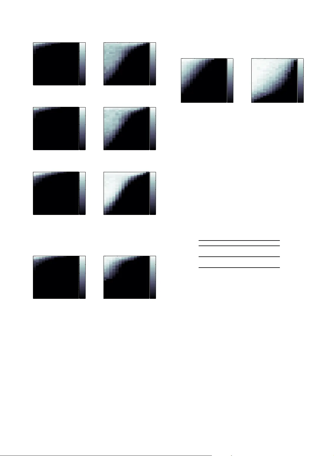
1 F ast Greedy Algor ithm f or Subspac e Cluster ing from Corr upted and Incomplete Data Ale xander P e tukhov , Inna K ozlov Abstract —We describe the F ast G reedy Sparse Subspace Clustering (FGSSC) algorithm providing an efficient method f or clustering data belonging to a f ew low-dimensional linear or affine subspaces. The main difference of our algor ithm from predecessors is its ability to w ork with noisy data having a high rate of er asures (missed entries with the kno wn coordinates) and errors (corrupted entries with unknown coordinates). The greedy approach consists in usage of a basic alg orithm on data out of the domain of the basi c algorithm reli ability . When the algorithm f ails and its output looses some desir able f eatures of the solution, usually it still brings some inf ormation about ”the largest features” of the solution. T he greedy algor ithm ext racts t hose f eatures and uses them in an iterativ e wa y by launching the basic algorithm with the additional information mined out on the previous iterat ions. Such scheme requires an addi tional time consuming algorithm loop. We d iscuss here how to implement the fast version of the greedy algorithm with the maximum efficiency whose greedy str ategy is incor porated into iterat ions of the basic algor ithm. We provide numerical evidences that, in the subspace clustering capab ility , the f ast greedy algorithm outperforms not only the ex isting state-of -the ar t SSC algor ithm taken b y the aut hors as a basic algorithm b ut also the recent GSSC algori thm. At the same time , its computational cost is only sli ghtly higher than the cost of SSC . The numerical e vidence of the algorithm significant adv antage is presented f or a f ew synthetic m odels as w ell as f or t he Extended Y ale B dataset of f acial images. In particular, the f ace recognition misclassific ation rate turned out to be 6–20 t imes lower than f or the SSC algorithm. We prov ide also the numerical evidence that the FGSSC algorithm is able to perf orm cluster ing of corrupted data efficiently ev en when the sum of subspace dimensions significantly e xceeds the dimension of the ambient space. Index Terms —S ubspace Clustering, Sparse Representations, Greedy Algorithm, Law- Rank Matrix Completion, Compressed Sensing, F ace Recognition ✦ 1 I N T R O D U C T I O N W e consider a greedy strategy based a lgorithm f or preprocessing on vector database necessary for sub- space clustering. The problem of subspace clustering consists in classification of the ve ctor data belong ing to a few linear or affine low-dimensional subspac es of the high dimensional ambient space when neither subspaces or even their dimensions are not known, i.e., they have to be identified f rom the sa me da tabase. No dataset for algorithm learning is provided. The problem has a long history and always was considered as difficult. In spite of its closeness to the problem of linear regress ion, the presence of multiple subspaces brings combinatorial non-polynomial com- plexity . A dditional hardness of the settings considered in this paper is due to the presence of combined artifacts consistin g of noise in the data , the errors at unknown loca tions. Moreover , a large data fra ction may be missed. There are many applied p roblems expecting the • A.Petukhov is with the Department of Mathematics, University of Georgia , Athens, GA, 306 02. E-mail: see http://www . math.uga.edu/˜petukhov • I.Kozlo v is C TO, Algosoft-T ech USA. progress in subspace clustering algorithm. A mong them the problems related to pro cessing of visual information are especially popular . T ypical pro blems are so rting da tabases consi sting of images taken from a finite set of objects like fa c es, character s, symbols. The special class of pr oblems is con stituted by motion segmentation p roblems which ca n be used for better motion estimation, vide o segmentation, and vide o 2D to 3 D conversion. The last successes in those areas a re connected with the recent Sparse Subspace Clustering algorithm developed in [8], [9 ] and thorough ly stud- ied in [21], [22]. Using more formal definition, we have N vectors { y l } N l =1 in K linear or affine subspaces S := { S l } K l =1 with the dimension s { d l } K l =1 of the D -dimensional Euclidean space R D . W e do not assume that those spaces do not have non-trivial intersections. However , we do assume that any one of those spaces is not a subspace of other one. At the same time, the situation when one subspace is a subspace of a sum of two or more subspaces from S is allowed. Such settings inspire the hope that when N is significantly la rge and the points are r andomly and independently dis- tributed on those planes some sophisticated algorithm can ide ntify those planes (subspaces) a nd classify the belongingness of each point to the found subspac e s. 2 Then the problem consists in finding a permutation matrix Γ such that [ Y 1 , . . . , Y K ] = Y Γ , where Y ∈ R D × N is an input matrix whose colum ns are the given points in an a rbitrary ra ndom order , whereas in [ Y 1 , . . . , Y K ] is rearra ngement of the matrix Y in the accordance with the affiliation of the vectors with the subspaces S k . Let us discuss restrictions on the input data a l- lowing expe c t some tractable output of the ”ideal” clustering a lgorithm provided that such algorithm exists. Any space S k defined by the cluster Y k has dimension a t most # Y k − 1 f or the linear spa ce settings and at most # Y k − 2 for the affine space settings. In addition to the dimension restriction, we req uire that any cluster Y k cannot be split into 2 or more clusters satisfying the dimension condition. Of course, some of points may belong to the in- tersection of two or more subspaces, then such point may be assigned to one of those subspaces or to all of them. However , it is reasonable to assume that, with probability 1, the points of Y belong to only one of subspaces from S . Summarizing discussion above, we formulate the precise model of the problem/algorithm input and what is an expected algorithm outcome. W e start with the input model. The pr oblem ”gen- erator” (synthetic or na tur a l) consi sts of 2 parts: gen- eration of subspaces and generation of da ta on those subspaces. While the subspaces from S can be generated ran- domly , they usually reflect the nature of the data and, in most ca ses, they can be described deterministically . The da ta in the matrix Y are formed as consecutive N times r a ndom selection of a subspace S k and then the random point belonging to it. W e assume that ra ndom generator has distribution having probability 0 for any proper linear (affine) subspace of S k . This property is instantly imply that almost f or sur e any selected vector of S k is a linear combination of other selected vectors from S k provided that the cardinality of that set exceeds d k by at least 1 (or 2). What is expected as an ideal algorithm outcome? If the p roblem gener ator provided us with a sufficient number of points belonging to the given space S k , we have right to expect that the a lgorithm will find the cluster Y k including a ll its points, when # Y k ≥ d k + 1 ( ≥ d k + 2) . Since the problem generator creates a finite number of points N , the probability that some of subspaces are not represented by a significant number of points is not zero. No algorithm is able to ide ntify such subspace for sure. So we have to a ssign those points as outliers . W e also may think about outliers as points genera te d randomly from e ntire space R D . It is convenient to put all outliers into additional set Y 0 not corresponding to any of spac e s f rom S and to agree that all spac e s in S k have enough representatives in { Y k } K k =1 . The problem of finding clusters { Y k } corresponding to linear/affine subspaces is solved usually by means of finding the clusters in the similarity graph whose edges ( to be more precise the weights of edges) char- acterize the interconnection between pairs of vertexe s. In our case, the popular method of clustering consists in making the points to play role of the vertexes, while the weights are set from the coefficients of decomposition of the vectors through other ve ctors from the same space S k . This idea loo ks as vicious circle. W e are trying to identify the spa c e S k accom- modating the ve c tor y i , using its linear decomposition in the remaini ng vectors from the ( not found yet) cluster Y k ⊂ S k . However , the situation is not hopeless at all. In [9], the exce llent suggestion to reduce the decomposition problem formulated above to solving the non-convex problem k c i k 0 → min , subject to y i = Y c i , c i,i = 0 , i = 1 , . . . , N ; (1) where k x k 0 is the Hamming weight of the vector x , k x k 0 := # { x j 6 = 0 } , was presented. The problem of finding the sparsest solutions to ( 1), so-called, Compressed Sensi ng or Comp r essive Sampling (CS), un- derwent thorough study originated in [4], [7], [20] and continued in hundr eds of theoretical and applied papers. W e have to emphasize that some requirem ents for the matrix Y a s well as topics of interest typical for CS settin gs are absolutely irrelevant to the problem above and may look too restrictive. Among those topics we mention the problem of the uniqueness of the solution to (1). Of course, the uniqueness of the solution is not important for us. Moreover , the minimization of the Hamming weight is difficult and may look unnecessar y in our case. Indeed, if the sum of the spaces S k is direct, any decomposition fits our request. In th is case, we ca n take, f or example, the least ℓ 2 -norm solutions. When the sum is n ot d irect the minimization of the Hamming weight be comes very helpful but still unnecessary . In the idea l world of perfect computational preci- sion a nd unlimited computational pow er , with prob- ability one, the solutions of (1) would point out the elements of the appropriate S l by their non-zero decomposition coefficients. Provided tha t no vectors of wrong subspaces participate in decomposition of each column of Y , the matrix C whose columns are c i allows perf ectly reconstruct the str ucture of the subspaces in polynomial time. There are two obstacles on that way . First, the precision of the input matrix Y is usually not perfect. So the d ecompositio ns may pick up wrong vectors even if we are ab le to solve problem (1). In this case, the pro blem of subspace clustering is considered for the similarity graph defined by the symmetric 3 matrix W := | C | + | C T | . While, generally spea king, this problem cannot be solved in polynomial time, there exist pra ctical algorithms allowing right clustering when the number of ”fa lse” interconnections of ele- ments from different subspaces are not very d ense and not very intensive. Follow ing [9], we will use some modification of the spectral clustering algorithm from [14] which is specified in [12] as ”gra p h’s random walk Laplacian”. The second obstac le consists in non-polyno mial complexity of problem (1) itself. The elegant solution allowing to overcome this obstacle is replacement of non-convex problem (1 ) with the convex pro blem k c i k 1 → min , subject to y i = Y c i , c i,i = 0 , i = 1 , . . . , N ; (2) or k C k 1 → min , subject to Y = Y C , diag ( C ) = 0; (3) in the matrix form. I t follows from the fundamental results from [4], [7], [20] that for matrices Y with some reasonable r estrictions on Y and for not very large Hamming weight of the ideal sparse solution, it can be uniquely found by solving convex problem (2). There are other more efficient ℓ 1 -based methods f or finding sparse solutions (e.g., see [5], [15], [10]). Provided that the data matrix is clean (maybe up to the noise in entries of not very high magnitude), the problem (3) ca n be so lved with the standard m ethods of Compressed Sensing. However , when some entries are corrupted or missed the special treatment of such input is necessary . W e note that while. when the the entries of the vector y i are corrupted, problem (2) can be efficiently solved with the algorithm f rom [16]. However , that algorithm requires a n uncorrupted matrix Y , what cannot be guaranteed in our case. The algorithm considered below does no t require clean input data . W e assume that those da ta may be corrupted with sparse e r rors, random noise is dis- tributed over all vector entries, and a quite significant part of data is missing. The property of errors to constitute a spar se set means that some (but not a ll) vector entries are cor - rupted, i.e., those values are randomly replaced with different values or some r andom errors a re added to the da ta entries. The locations (indexes) of the corrupted entries are unknown. The second type of the corruption is mis sing data. In information theory , the missed samples are ca lled erasures. They have two main features. First, the data va lues in e r asures d oes not have any practical importance. The most natural way is to think about erasures as a bout lost data. Second, the coordinates of erasures are known. The second fe ature is the main difference with errors. The noise is randomly intro duced in each entry . Its magnitude is usually much less than the data magni- tude. T wo main sources of the noise are imperfect data measuring and finite precision of data r epresentation. It should be mentioned, that the matrices Y in pra c- tical problems may be very far from the requirements for the uniqueness of solution s. At the same time, the uniqueness of the solut ions, as we mentioned a bove, is not necessary in our settings. The error correction as well as erased entries recovery are also not crucial for the final goal of th e clustering. W e just wis h to have the maximum of separation betwee n indexes of the matrix W corresponding to different subspaces. In the case of successful clustering, the results for each S k may be used for further processing like data noise removal, error correction, and so on . Such procedures become significantly mor e efficient wh en applied to low-rank submatrices of Y c orrespon ding to one subspace. Thus, in app lications, the problems involving sub- space clustering can be split into 3 stages: 1) preprocessing (graph W composing); 2) search f or clusters in the graphs; 3) processing on c lusters. In this paper , we develop a first stage a lgorithm helping to perform the second stage much more ef - ficiently than the state- of-the-art algorithms. In [18 ], we designed the Greedy S parse S ubspace Clustering (GSSC) algorithm relying on main principles of SS C algorithm from [9] but having increased clustering capabilities due to implementation of greedy ide a s at cost of the high er (about 5 times) computational complexity . Here we present an accelerated version of GSSC which is not slower than SS C. As for its capability to separa te subspa c es, we will show it outperforms (sometimes significantly) not only SSC but even GSSC. W e will call this algorithm the Fast GSSC or FGSSC. W e d o not discuss any aspects of improvements of stage 2. W e just take one of such algorithms, specifi- cally the spectral c lustering, a nd use it for comparison of the influence of our and competing preprocessi ng algorithms on the efficiency of clustering. As for stage 3, its content depends on an a pplied problem req uesting subspace clustering. The data r e- covery fro m incomplete and corr upted measuremen ts is one of typica l possible goals of the thir d stage. Sometimes this problem is called ”Netflix Prize prob- lem”. W e will briefly discuss below how the sa me problems of incompleteness a nd corruption can be solved within clustering p repr ocessing. However , for low-rank matrice s (found clusters) it can be solved more efficiently . Among many existing algorithms we mention the most recent papers [3], [6] [11], [23], [24], [17] pro viding the best results for input having both erasures and er rors. It should be mentioned that in the ca se when dim( P S k ) < D the inverse order of steps ca n be applied. On the step, the matrix Y is completed and corrected with one of algorithms mentioned in the previous paragraph. Then the clean matrix Y can 4 be processed with SSC algorithm. Of coarse, this approach fails when d := dim( P S k ) is comparable or greater than D . It a lso is unr eliable when we do not know the value d in advance. In S ection 2, we discuss the formal settings of optimization problem to be solved. In Sections 3.1 we discuss the algorithm SSC ( [ 9]) and our modification ([18]) allowing to work with incomplete matrice s. In Section 3.2, we describe the Greedy SSC (GSSC) algorithm constructed in [18] as exter na l constru ction over SSC. In Section 3.3, we introduce the Fast GSSC (FGSSC) algorithm which is the main topic of this paper . The resul ts of numerica l experiments showing the consistency of the proposed approach for both synthetic and real world data will be given in Sec- tion 4. 2 P R O B L E M S E T T I N G S W e use main features of Sparse Subspace Clustering algorithm (S S C) from [9] for our modification based on a greedy approach. Some a d ditional e xtended reasoning related S SC can be found in [9] and in the earlier paper [8]. The SSC a lgorithm in its last form created the tool for subspac e clustering resilient to data errors. In [18], we adapted the S SC algorithm to the ca se when p a rt of d ata is missing a llowing successful clustering even if a significant f raction of data is unavailable. The same mechanism provides a tool for more e fficient error resilience. V ery similar to SSC ideas of subspace self- representation for subspace clustering were used also in [19]. However , the error resili ence mechanism in that paper works under a ssumption tha t there are enough uncorrupted data ve ctors. This assumption is the case for the S SC a lgorithm selected as a foundation for GSSC. Optimization CS problems (2) and (3) assume that the data are clean, i.e., they hav e no noise and er- rors. Considering the problem within the standard CS fra mework, in the presence of e rrors, the prob- lem 1 can be reformulated a s finding the sparsest vectors c ( decomposition coefficients) and e (errors of ”mesurements”) satisfying the system of linear equations y = A c + e . It was mentioned in [23] that the last system can be re-written a s y = [ A I ]  c e  , (4) where I is the identity matrix. Therefor e, the prob- lem of sparse reconstructio n and error correction ca n be solved simultaneously with CS methods. In [16], we designed an algorithm efficiently finding spar se solutions to (4). Unfortunately , the subspace c lustering algorith ca n- not a dopt this strategy straightforwardly because not only ”measurements” y i are corrupted in ( 1) but ”measuring matrix” A = Y also can be corrupted. It should be mentioned that if the error probability is so low that there exist uncorrupted columns of Y consti- tuting bases for all subspaces { S k } , the method from [16] can solve the problem of sparse repr esentation with simultaneous error correction. In what follows, the c onsidered algorithm will admit a significantly higher error rate. In particular , all columns of Y may be corrupted. Now we describe optimization settings accepted in this paper . Following [9], we introduce two (unknown for the problem solver) D × N matrices ˆ E a nd ˆ Z . The matrix ˆ E contains a sparse (i.e., # { E ij 6 = 0 } < DN ) set of erro rs wi th relatively large magnitudes. The matrix ˆ Z defines the noise having a relatively low magnitude but distributed over all entries of ˆ Z . Thus, the clean data a re representable as Y − ˆ E − ˆ Z . Therefor e, when the data are corrupted with sparse errors a nd noise, the equation Y = Y C has to be replaces by Y = Y C + ˆ E ( I − C ) + ˆ Z ( I − C ) . (5) The authors of [9] applied a reasonable simplification of the problem by replacing 2 last terms of ( 5) with some ( unknow n) sparse matrix E := ˆ E ( I − C ) and the matrix with the deformed no ise Z = ˆ Z ( I − C ) . Provided that the sparse C e xists, the matrix E still has to be spar se. This transformation lea ds to some simplification of the optimization procedure. This is admissible simplification since, generally speaking, we do not need to c orrect a nd denoise the input data Y . Our only goal is to find the sparse matrix C which is a building block for the matrix W . Therefore, we do not need matrices ˆ E a nd ˆ Z . While ther e is an option to apply the erro r c orrec- tion procedure after subspace clustering, the problem of incorporation of th is procedure, i.e. , the matrices ˆ E and ˆ Z , into subspace clustering still makes sense and d e serves consideration in the future. However , it will be clear from what follows that straightforward incorporation leads to unj ustified complexification of the optimization procedures. T a king into ac c ount the simplification from above reasoning, we ca n formulate the constrained optimiza- tion problem min k C k 1 + λ e k E k 1 + λ z 2 k Z k 2 F , s.t. Y = Y C + E + Z , diag ( C ) = 0 . (6) where k · k F is the Frobenius matrix norm. If the clus- tering in to affine subspaces is required, the additional constrain C T 1 = 1 is added. On the next step, using the representation Z = Y − Y C − E and introducing an auxiliary matrix A ∈ R N × N , constrained optimization pr oblem (6) is transformed into min k C k 1 + λ e k E k 1 + λ z 2 k Y − Y A − E k 2 F s.t. A T 1 = 1 , A = C − diag ( C ) . (7) 5 Optimization problems (6) a nd (7) are equivalent. Indeed, obviously , at the point of the extremum of (7), diag ( C ) = 0 . Hence, A = C . At last, the quadra tic penalty functions with the weigh t ρ/ 2 corr esponding to constrains are add ed to the functional in (7) and the Lagrangian functional is composed. The final Lagrangian functional is as follows L ( C, A, E , δ , ∆) = min k C k 1 + λ e k E k 1 + λ z 2 k Y − Y A − E k 2 F + ρ 2 k A T 1 − 1 k 2 2 + ρ 2 k A − C + diag ( C )) k 2 F + δ T ( A T 1 − 1 ) + tr (∆ T ( A − C + diag ( C ))) , (8) where the vector δ and the matrix ∆ are Lagra ngian multipliers. Obviously , since the penalty functio ns are formed from the constrains, they do n ot change the point and the value of the minimum. The first terms in lines 3 and 4 of (8) have to be remo ved when only linear subspace clusters a re considered. 3 A L G O R I T H M S 3.1 Sparse Subspace Clustering Algorithm For finding the stationary point of functio nal (8) a n Alternating Dir ection Method of Multipliers ( ADMM, [1]) is used. In [9], this pro cedure is a crucial pa r t of the e ntire algorith m which is ca lled the S p a rse Sub- space Clustering algorithm. While this minimization constitutes only a part of the entire S SC algorithm, for the sake of brevity , we will call it the SSC algorithm. Before formal description of the SSC algorithm we discuss the selection of parameters in (8). The parameters λ e and λ z in (8) are selec te d in advance. They define the compromis e between good approximation of Y with Y C and the high spa r sity o f C . The general rule is to set the larger values of the parameters f or the less level of the noise or errors. In [9], the selection of the parameters by formulas λ e = α e /µ e , λ z = α z /µ z , (9) where α e , α z > 1 and µ e := min i max j 6 = i k y j k 1 , µ z := min i max j 6 = i | y T i y j | , is recommended. The initial parameter ρ = ρ 0 is set in a dvance. It is upd a ted as ρ := ρ k +1 = ρ k µ with itera tions of SSC algorithm. W e notice that, add ing the penalty terms, we do not change the problem. It still has the same minim um. However , the appropriate selection of µ and ρ 0 accelerates the algorithm convergence significantly . W e will need the follow ing notation S ǫ [ x ] :=    x − ǫ, x > ǫ, x + ǫ, x < − ǫ, 0 , otherwise ; where x ca n be either a number or a vector or a matrix. The operator S ǫ [ · ] is called the shrinkage operator . In what follows, we accept that the d ata (matrix Y ) is availab le only a t entries with indexes on the set Ω ⊂ { 1 , . . . , D } × { 1 , . . . , N } . χ Ω is a characteristic function of the set Ω . The symbol ⊙ will be used for the entrywise products of matr ices. Algorithm 1 SSC ( modified) Input: Y ∈ R D × N , Ω ∈ R D × N . 1: Ini tializa tion: C 0 := 0 , A 0 := 0 , E 0 := 0 , δ 0 := 0 , ∆ 0 := 0 , k := 0 , STOP:=false, ǫ > 0 , ρ 0 > 0 , µ ≥ 1 2: whi le STOP== false do 3: update A k +1 by solvi ng the system of lin ear equations ( λ z Y T Y + ρ k I + ρ k 11 T ) A k +1 = λ z Y T ( Y − E k ) + ρ k ( 11 T + C k ) − 1 δ kT − ∆ k . (10) 4: update C k +1 := J k − diag ( J k ) , where J k := S 1 /ρ k [ A k +1 + ∆ k /ρ k ] . 5: update E k +1 := χ Ω ⊙ S λ e λ z [ Y − Y A k +1 ]+ (1 − χ Ω ) ⊙ ( Y − Y A k +1 ) (11) 6: update δ k +1 := δ k + ρ k ( A k +1 1 − 1 ) , 7: update ∆ k +1 := ∆ k + ρ k ( A k +1 − C k +1 ) . 8: if k A k +1 1 − 1 k ∞ < ǫ , & k A k +1 − C k +1 k ∞ < ǫ , & k A k +1 − A k k ∞ < ǫ , & k E k +1 − E k k ∞ < ǫ then STOP=true; 9: end if 10: update ρ k +1 := ρ k µ 11: update k := k + 1 12: e nd while return C ∗ = C k , Y out := Y − E k . Each iter ation of the algorithm is based on consecu- tive optimization with respect to each of the unknown values A , C , E , δ , ∆ which are initialized by zeros before the a lgorithm starts. Due to an appropriate form o f f unctional (8), op- timization of A k , C k , and E k in Algorithm 1 is simple and computationally efficient. Moreover , lines 3–5 give the optimal (for the fixed other varia b le s) solution in the explicit form. The five formulas (lines 6 3–7) f or updating the unknown values a re discussed below . The matrix A k +1 is a solution of the matr ix equation with the unk nown matrix of size N × N . However , when D < N , the complexity of this operation is below O ( N 3 ) . Indeed, obviously , ( λ z Y T Y + ρI + ρ 11 T ) − 1 = ρ − 1 ( I + ˜ Y T Q − 1 ˜ Y ) , (12) where ˜ Y =    Y , case of linear subspaces;  Y 1 T  , case of affine subspa ces; Q = V + ˜ Y ˜ Y T ∈ R D × D ( or R ( D +1) × ( D +1) ) , V is a d iagonal matrix, V ii = ρ/ λ z , i = 1 , . . . , D ; V D +1 ,D +1 = 1 for the ca se of affine subspaces. In typical cases, the number of points N is much greater than the dimension of the ambient spa c e D . Thus, th e complexity of the matrix inversion in (12) is O ( D 3 ) . Computation of the matrix Q requir es O ( D 2 N ) operations but, in fact, computi ng Y Y T has to be performed only on the first iteration of Algorithm 1. Unfortunately , the follow-up matrix multiplication has complexity O ( D N 2 ) . Nevertheless, p rovided that D ≪ N , computing of the solution to (1 0) may be much faster than the straightforward solving that system. Lines 4 a nd 5 of A lgorithm 1 represents explicit optimization of the functional (8) with respect to C and E correspondingly , provided that other variables are fixed. Lines 6 and 7 present upd ates of the La grangian multipliers δ and ∆ . Those updates do not solve any optimization problems. Their intention is to mo ve the value of the Lagrangian functional toward it mini- mum value. More derailed arguments and discussion related to Alternating Direction Method of Multipliers justifying this step can be found in [1]. Algorithm 1 is a modified version of the original SSC algorithm from [9] which gave the sta te-of-the- art benchmarks for subspace clustering problems. Our first modification consists in taking into a c- count missing data by means of replacing the update formula E k +1 := S λ e λ z [ Y − Y A k +1 ] with our ve rsion (11). T o make clear how that modification use the a priori knowledge of the coor dinates of erased entries, let us consider the mechanism of the influence of the va lue λ e on the output matrix C . The para meter λ e sets the b a lance between the higher level of the spa rsity of C with the more popula te d error matrix E v s. the less spa rse C and the less populated matrix E . Setting too small λ e allows too many ”errors” and very sparse C . However , probably , this is not what we want. This woul d mean that sake of C spar sity we introduced too large distortion into the input data Y . At the same time, if we know for sure or almost for sure that some entry of Y with coor dinates ( i, j ) is corrupted, we loose nothing by assigning to this element an individual small weight in functional (8). This weight can be much less than λ e or eve n equal to 0 . Thus, we have to replace the term k E k 1 with k χ Ω ⊙ E k 1 . This means tha t in formula (11) we ap ply different shrinkage threshold for different indexes. Generally speaking, it ma ke s sense to use all range of non-negative real numbers to reflect our knowledge about E . Sa y , highly reliable entries have to be pro tected from d istortion by the weight greater than 1 . However , in this pape r we restrict ourself with two-level e ntries: either 1 (no knowlege) or 0 (erasure or entries suspici ous to be errors), using the characteristic function χ Ω for reweighti ng. In the case when no erasures are reported, we have χ Ω ≡ 1 . Ther efore, Algorithm 1 at line 5 works like a regular SSC algorithm . Our second modification of S SC consists in updat- ing ρ (line 10 ). As we can judge, no upda te was used in the original algorithm in [9]. While such update does not change the optimal value of the functional, it brings some algorithm accelera tion. In Sec tion 4, we will give numerica l evidences of the efficiency of Algorithm 1 for fighting the problem of missing samples. 3.2 Greedy Sparse Sub space Clustering While the origin al S SC algorithm in [9] did not have any special tool against missing samples, it engaged the error resilience mechanism. In particula r , it can perform clustering on data with some restricted num- ber of era sures. However , by our opinion, the poten- tial power of the error resilience laid in Algorithm 1 was no not realized completely . The main ide a lying in the foundation of our follow- up reasoning is a sim ple in formation theory principle. Assume that in the beginning no information about errors in da ta is available. Then if we a re able (say , using one run of the SSC algorithm) to identify that some data entries contain errors, the errors can be re- qualified into erasures (marked as erasures) and run the algorith m working ef ficiently with erasures again. Our intuitio n ba ses on information theory principles tells us that any e xtra knowledge (say , coordinates of errors) has to give some benefits f or algorithm. At the same time, this strate gy has some r estrictions. Let us discuss how this trick may change (hopefully improve) our algorithm. First of all, we have to be sure that w e found and marked actual errors. M oving ”healthy” entries into the list of erasures, we destroy correct information and reduce the algorithm ability to make reliable c onclusions. Thus, the procedure of finding the error loca tions has to be reliable. However , even if we are able to find correct er ror locations, we have to take into account that re-qualification of 7 errors into era sures implies the necessity to accept that the value at the erroneous entries do not contain any usef ul information. Such claim is tru e only if the v a lues at e rror locations are independent from each other a nd from the correct values. The most typical ca se when those independence requirements fail is the mixture of data with noise. While all e ntries are corrupted, they still have information about data which can be used for d a ta recovery . At the same time, moving a data entry into the list of era sures we lose tha t useful information. Thus, the idea of moving the errors into the list of erasures may bring benefits only when the algorithm of finding error locations is consisten t and amount of usef ul information in corrupted entries is not too large. In spite of the mentioned above restrictions, in many cases, incomplete information can be processed more efficientl y than erroneous information. Our suggestion is to attract ideas of greedy a lgo- rithms to increase the capa bility of the SSC algorithm in subspace clustering. Greedy algorithms are ver y popular in non-linear approximation (especially in redundant systems) when the global optimization is replaced with iterative selection of the most probable candidates from the point of view of their pr ospective contribution into a pproximation . The procedure is repeated with selection of new entries, considering the previously selected entries a s reliable with guaranteed participation in a p proxim ation. The most typical case is Orthogo nal Greedy A lgorithm ( OGA) consisting in selection of the approximating entries ha v ing the biggest inner pro ducts with the current approxima- tion residual and follow-up orthogonal projection of the approximated object onto the span of the selec te d entries. In many cases, OG A a llows to find th e sparse st r ep- resentations if they exist. In [ 10] and [ 15], we a pplied the greedy idea in combination with the reweighted ℓ 1 -minimization to CS problem of finding the sparsest solutions of underdetermined system. W e used the existing ℓ 1 -minimization scheme from [5] with the the opportunity to reweight entries. When the ba sic algorithm fails, the greedy block picks locations of the b iggest (the most reliable) entries in the decom- position whose magnitudes are higher than some threshold. Those entries a re considered as r eliable. Therefore, they get the less weight in the ℓ 1 -norm while other e ntries are competing on next itera tions for the right to be picked up. The similar idea was employed in our recent paper [17], where the greedy a pproach was applied to the algorithm for completion of low-rank matrices from incomplete highly corrupted samples from [ 11] based on the Augmented Lagrange Multipliers metho d. The simple greedy modification of the matrix completion algorithm from [1 1] gave the boost in the algorithm restoration capability . Now we discuss details how the greedy approach can be incorporated in (to be more precise ov er ) the SSC algorithm (cf . [18]). As above, we use the set Ω for keeping the information about erasures. However , we a lso will use it as a storage of information about coordinates of presumptive er rors. Such information will be extracted from the erro r ma tr ix E . Thus, χ Ω vanishes at the selected in ad vance erasures a nd at the points suspicious to be errors. The entries which are suspicious to be errors are dynamically removed from Ω after e a ch itera tion of the greedy a lgorithm. Algorithm 2 GSSC Input: Y ∈ R D × N , Ω ∈ R D × N . 1: Ini tializa tion: Y 0 := Y ⊙ χ Ω , Ω 0 = Ω , 0 < α 1 , α 2 , β < 1 , maxIter > 0 , k := 0 , STOP:=false. 2: mxM ed := max 1 ≤ j ≤ N median ( | y j | ) ; 3: whi le STOP== false do 4: ( C k , Y out ) = SSC ( Y k , Ω k ) ; 5: E = | Y out − Y k | ; 6: if k == 0 the n 7: M := max { α 1 · ma x { E } , α 2 · mxMed } ; 8: end if 9: M := β M ; 10: Ω k +1 := Ω k \ { ( i, j ) | E i,j > M } ; 11: Y k +1 := χ Ω k +1 ⊙ Y k + (1 − χ Ω k +1 ) ⊙ Y out ; 12: if k == maxIter the n 13: STOP:=true; 14: end if 15: k := k + 1 ; 16: e nd while Output: C k − 1 . Thus, in the Greedy Spa rse Subspace Clustering (GSSC), we organize an external loop over the SSC. One iteration of our greedy algorithm consists in running the modified version of SSC a nd Ω a nd Y updates. While E n in Algorithm 1 is not a genuine matrix of errors, this is not serious drawback for the original SSC algorithm. However , f or GSSC this may lead to unjustified and very undesira ble shrinkage of the set Ω . A more accurate estimate of the error set in future algorithms may bring significant benefits for GSSC. 3.3 Fast Greedy Sparse Subspace Clustering Al- gorithm Now we present the Fast Greedy Sparse Subspace Clustering ( FGSSC) algorithm (see Algorithm 3 ) which is main contribution of this paper . The FGSSC consists in in corporation of the greedy update of the set Ω into Algorithm 1. Except for the obvious elimination of the exter- nal GSSC loop leading to the acceleration of the algorithm, accurate tuning of the FGSSC pa rameters brings quite significant increase of the a lgorithm ca- pability . 8 Algorithm 3 FGSSC Input: Y ∈ R D × N , Ω ∈ R D × N . 1: Ini tializa tion: C 0 := 0 , A 0 := 0 , E 0 := 0 , δ 0 := 0 , ∆ 0 := 0 , k := 0 , M = ∞ , STOP:=false, ǫ > 0 , ρ 0 > 0 , µ ≥ 1 2: mxM ed=median ( χ Ω ⊙ Y ) ; 3: whi le STOP== false do 4: if k == k 0 then M := α 0 k E ij k ∞ ; 5: else 6: if k is even then 7: M := max { α 1 M , α 2 mxMed } ; 8: end if 9: end if 10: Ω := Ω \ { ( i, j ) | | E i,j | > M } ; 11: update A k +1 by solvi ng the system of lin ear equations ( λ z Y T Y + ρ k I + ρ k 11 T ) A k +1 = λ z Y T ( Y − E k ) + ρ k ( 11 T + C k ) − 1 δ kT − ∆ k . 12: update C k +1 := J k − diag ( J k ) , wher e J k := S 1 /ρ k [ A k +1 + ∆ k /ρ k ] . 13: update E k +1 := χ Ω ⊙ S λ e λ z [ Y − Y A k +1 ]+ (1 − χ Ω ) ⊙ ( Y − Y A k +1 ) 14: update δ k +1 := δ k + ρ k ( A k +1 1 − 1 ) , 15: update ∆ k +1 := ∆ k + ρ k ( A k +1 − C k +1 ) . 16: if k A k +1 1 − 1 k ∞ < ǫ , & k A k +1 − C k +1 k ∞ < ǫ , & k A k +1 − A k k ∞ < ǫ , & k E k +1 − E k k ∞ < ǫ then STOP:=true; 17: end if 18: if k is e ven then 19: Y := Y − χ Ω E k ; 20: E k +1 := 0 ; 21: update µ e (Ω) and µ z (Ω) ; 22: end if 23: update ρ k +1 := ρ k µ 24: update k := k + 1 25: e nd while return C ∗ := C k Now we give comments on A lgorithm 3 implemen- tation. FGSSC starts with a f ew iteration with blocked update of the set Ω . A very large value is set at the threshold for upda te M . It gets a realistic value (see line 4) after k 0 iterations. Those initial k 0 -step tuning allows to fill erasures with some reasonable values approximating ”genuine” values of Y . Those steps also provide us with an estimate of the largest values of errors. The algorithm iterations are grouped in pairs. After even iterations the estimate of the error matrix E accumulated for 2 itera tion is subtracted from the data matrix Y (line 18). After that, E is set to 0 . Updates of µ e (Ω) and µ z (Ω) in line 21 are optional they makes a sense when Ω has significant change during iterations and erroneous entries may have large ma gnitudes. The number of erasures ( and eve n their coordi- nates) is known before the p rocessi ng. So some of the a lgorithm para meters can be tuned, according to the known in formation. The parameters α e , α z can be used for the algorithm fine a djustment to the erasure density of the input data. 4 N U M E R I C A L E X P E R I M E N T S In the beginning, we will present the comparison of the FGSS C and SSC a lgorithms on two types of syn- thetic data. The third part of this section is devoted to the problem of the face recognition. T o be more precise we consider face images classification problem and present comparison of the FGSSC and SSC algorithms. For the paper siz e reduction, we do not present the results of GSSC algorithm which can be found in our paper [1 8]. W e just mention that it provides the clustering efficiency approximately in the middle between SSC and FGSSC a nd its exe cution time is 2-3 times greater tha n that time for FGSSC. W e also have to emphasize that in this paper we do not try to intrude into the spectr a l clustering algorithm. W e just provide equal opportunity for the SSC and FGSSC algorithms for the final cluster selection based on the matrices C obtained by ea ch of algorithms. For this reason we do not discuss here some important topics like data outliers . 4.1 Synthetic Input I The input d ata for the first experiment was c omposed in a ccordance with the model given in [9]. 10 5 data vectors of dimension D = 50 are equally split between three 4-dimensional linear spaces {S i } 3 i =1 . T o make the problem more complicated ea ch of those 3 spaces belongs to sum of two others. The smallest angles between spaces S i and S j are defined by f ormulas cos θ ij = max u ∈S i , v ∈S j u T v k u k 2 k v k 2 , i, j = 1 , 2 , 3 . W e construct the data sets usin g vectors generated by decompositions with random coefficients in orthonor - mal bases e j i of the spaces S j . Three vectors e j 1 belong to the same 2D-plane with angles d e 1 1 e 2 1 = d e 2 1 e 3 1 = θ and d e 1 1 e 3 1 = 2 θ . The vectors e 1 2 , e 2 2 , e 1 3 , e 2 3 , e 1 4 , e 2 4 are mutually orthogonal and orthogonal to e 1 1 , e 2 1 , e 3 1 ; e 3 j = ( e 1 j + e 2 j ) / √ 2 , j = 2 , 3 , 4 . The generator of standard normal distribution is used to genera te data decom- position coefficients. A fter the generation, a random unitary matrix is applied to the result to avoid zeros in some regions of the matrix Y . W e use the notation P ers and P err for probabilities of erasures and er rors correspondingly . 9 When we generate erasures we set random entries of the matrix Y with probability P ers to zero since no a priori information about those values is known. The coordinates of samples with errors a re gen- erated randomly with probability P err . W e use the additive model of errors, adding values of errors to the correct entries of Y . The magnitudes of e r rors are taken from standard normal distribution. Obviously , as we discussed in Section 3.2, f or such a dditive model the corrupted entries contain a lot of usef ul informa- tion about the data and potentially may be processed better than with our FGSSC algorithm. However , in spite of that, we will see below that impr ovement of clustering efficiency over SSC is significant. W e run 50 trials of FGSSC and SSC algorithms for each combination of ( θ , P err , P ers ) , 0 ≤ θ ≤ 60 ◦ , 0 ≤ P err ≤ 0 . 5 , 0 ≤ P ers ≤ 0 . 7 , and output average values of misclassification. W e note that f or the angle θ = 0 the spaces {S l } have a com mon line and dim( ⊕ 3 l =1 S l ) = 7 . Ne vertheless, we will see that SSC a nd espec ia lly GSSC shows high capability even for these hard settings. Pers Perr SSC, θ =0 o , no noise 0 0.2 0.4 0.6 0 0.1 0.2 0.3 0.4 0.5 0.4 0.3 0.2 0.1 0.0 Pers Perr FGSSC, θ =0 o , no noise 0 0.2 0.4 0.6 0 0.1 0.2 0.3 0.4 0.5 0.4 0.3 0.2 0.1 0.0 Pers Perr SSC, θ =6 o , no noise 0 0.2 0.4 0.6 0 0.1 0.2 0.3 0.4 0.5 0.4 0.3 0.2 0.1 0.0 Pers Perr FGSSC, θ =6 o , no noise 0 0.2 0.4 0.6 0 0.1 0.2 0.3 0.4 0.5 0.4 0.3 0.2 0.1 0.0 Pers Perr SSC, θ =60 o , no noise 0 0.2 0.4 0.6 0 0.1 0.2 0.3 0.4 0.5 0.4 0.3 0.2 0.1 0.0 Pers Perr FGSSC, θ =60 o , no noise 0 0.2 0.4 0.6 0 0.1 0.2 0.3 0.4 0.5 0.4 0.3 0.2 0.1 0.0 Fig.1. Clustering on noise free input. Now we describe the algorithm parameters. SSC processing was perf ormed with α e linearly changing from 5 (no erasures) to 24 for 0. 7 erasures. α z = 7 , ρ 0 = 10 , µ = 1 . 05 , ǫ = 0 . 001 . The results for the FGSSC algorithm presented on Fig. 1 were obtained with parameters α 0 = 0 . 6 , α 1 = 0 . 95 , α 2 = 1 . 0 ; the parameter α e is linearly changed from 11 for P ers = 0 . 0 to 22 for P ers = 0 . 7 ; α z = 20 . Each point of the images is obtained as avera ge value over 50 trials when both the matrix Y , sets of erasures and errors as well as the va lues of errors are randomly drawn, according to the models described above. The intensity of each point takes a range from ”white”, when there is no e rrors in clustering, to ”blac k” , when more than 50% of vectors were misclassified. The results confirms that FGSSC has much higher error/erasure resilience than SSC. For a ll models of input data and for both algorithms ”the phase tr a nsi- tion curve” is observed. For the case θ = 0 ◦ , clustering cannot b e absolutely perfect even for FGSSC. Indeed, the clustering for P err > 0 and P ers > 0 cannot be better than for error f ree model. At the sa me time, FGSSC was designed for better error handling. In the error free ca se, FGSS C has no advantage over the SSC algorithm. Thus, the images on Fig. 1 for θ = 0 have th e gray ba ckgroun d of the approximate leve l 0 . 042 equal to the rate of mis classification of S SC. W e believe that the reason of the misclassification lies in the method how we define the success. For θ = 0 ◦ , there is a common line (a 1 D subspace) belonging to all subspaces S l . For points close to that line, the c onsidered algorithm has to make a hard decision, appointing only one cluster for each such point. Probably , for most of a p p lied problems , the in- formation about multiple subspaces accommodation is more useful than the unique spac e sele c tion. W e advocate for such mul tiple selection because the typi- cal follow-up problem after clustering is correction of errors in eac h of clusters. For this problem, it is not important to which of clusters the vec tor belonged from the beginning. When the vector affiliation is really important, side information has to be attracted. The second pa rt of experiment de als with noisy data processing. Independent Gaussian noise of mag- nitude 10% of mean square value of the data matrix Y (i.e., the noise level is -20dB) is applied to the matrix Y . On Fig. 2, we present the results of processing of the noi sy input analogous to results on Fig. 1. Evi- dently , that this quite strong noise has minor influence on the clustering efficiency . If we increase the noise up to -1 5 d B , the algorithms still r esist. For -10 dB (see Fig. 3) FGSS C looses a lot but still significantly outperforms SSC. Those lo sses are obviously caused by the increase of the noise fraction in the mixtur e errors-erasures-noise, while the greedy idea efficiently works f or highly localized corruption like errors a nd er asures. 10 Pers Perr SSC, θ =0 o , noise −20 dB 0 0.2 0.4 0.6 0 0.1 0.2 0.3 0.4 0.5 0.4 0.3 0.2 0.1 0.0 Pers Perr FGSSC, θ =0 o , noise −20 dB 0 0.2 0.4 0.6 0 0.1 0.2 0.3 0.4 0.5 0.4 0.3 0.2 0.1 0.0 Pers Perr SSC, θ =6 o , noise −20 dB 0 0.2 0.4 0.6 0 0.1 0.2 0.3 0.4 0.5 0.4 0.3 0.2 0.1 0.0 Pers Perr FGSSC, θ =6 o , noise −20 dB 0 0.2 0.4 0.6 0 0.1 0.2 0.3 0.4 0.5 0.4 0.3 0.2 0.1 0.0 Pers Perr SSC, θ =60 o , noise −20 dB 0 0.2 0.4 0.6 0 0.1 0.2 0.3 0.4 0.5 0.4 0.3 0.2 0.1 0.0 Pers Perr FGSSC, θ =60 o , noise −20 dB 0 0.2 0.4 0.6 0 0.1 0.2 0.3 0.4 0.5 0.4 0.3 0.2 0.1 0.0 Fig.2. Clustering on noisy in put, S NR=20 dB. W e e mphasize that a ll results on Figs. 1– 3 were obtained with the same algorithm settings. Pers Perr SSC, θ =60 o , noise −10 dB 0 0.2 0.4 0.6 0 0.1 0.2 0.3 0.4 0.5 0.4 0.3 0.2 0.1 0.0 Pers Perr FGSSC, θ =60 o , noise −10 dB 0 0.2 0.4 0.6 0 0.1 0.2 0.3 0.4 0.5 0.4 0.3 0.2 0.1 0.0 Fig.3. Clustering on noisy in put, S NR=10 dB. 4.2 Synthetic Input II W e put our data into the ambient space of the same dimension D = 50 as in Section 4.1. However , we no w use the model with absolutely r a ndom selection of subspace orientations. W e fix the number of subspaces K = 7 but the dimensions of subspaces are selected randomly within the ra nge 3 ÷ 10 . In particular , those settings mean that the ex pectation of subspac e dimen- sions is 6.5 . Therefore, the total average dimension (the sum of all dimensions) of a ll subspace is close to the dimension of the entire ambient space. The number of data points is set as N = 200 . Those points are randomly distributed between planes. The number of p oints in each subspace does not depend on their dimensions. However , to de fine a cluster and avoid obvious outliers the num ber of points per each subspace has to e xceed the dimension of that subspace. Pers Perr SSC, 7 random subspaces 0 0.2 0.4 0.6 0 0.1 0.2 0.3 0.4 0.5 0.4 0.3 0.2 0.1 0.0 Pers Perr FGSSC, 7 subspaces. D=50 0 0.2 0.4 0.6 0 0.1 0.2 0.3 0.4 0.5 0.4 0.3 0.2 0.1 0.0 Fig.4. Clustering on 7 subspace model. The parameter α e has lin ear dependency fr om P ers : α e := β 1 + β 2 P ers , whereas the dependence of α z is quadratic: α z = γ 1 + γ 2 P 2 ers . The para meters are given in the T able 1 . The pa ram- eters as well as the formulas were found empirically . T ABLE 1 Algorithm P arameters D = 15 D = 25 D = 50 β 1 5 5 7 β 2 36 22 18 γ 1 0.7 0.8 3 γ 2 29 10.8 6.8 Now we present r esults of two experiments with the lower dimension of the ambient space. Fig. 4 gives indirect hint about approxim ate possible dimension reduction. Indeed, on Fig. 4, we see that not perfect but decent FGSSC clustering is possible when only 30% of data entries are availa ble. Erasing 70% of the data entries in a vector can be interpreted a s an orthogonal projection on the spa ce ha ving lower dimension. In fact, introducing ra ndom e rasures we just project our data on random coordinate planes. If, instead of random erasures, we era se the 70% of each data vector entries with the greatest index e s, we also have an orthogonal projection of a ll vectors on the same linear space. While this pr ocedure defines de - terministic erasure which could lead to ”systematic” drawbacks for some specific input, in our data model, the r andomness is guaranteed by the input d a ta. This non-rigo rous common sense reasoning allows to expect that the reduction of the a mbient spa ce dimension at least up to 15 = 50 × 0 . 3 is ” e quivalent” to 7 0% erasures for the data in R 50 . The result of the experiments for D = 15 and D = 25 are given on Fig. 5 and Fig. 6. They support our reasoning above. 11 Pers Perr FGSSC, 7 subspaces. D=15 0 0.2 0.4 0.6 0 0.1 0.2 0.3 0.4 0.5 0.4 0.3 0.2 0.1 0.0 Pers Perr FGSSC, 7 subspaces. D=25 0 0.2 0.4 0.6 0 0.1 0.2 0.3 0.4 0.5 0.4 0.3 0.2 0.1 0.0 Fig.5. Clustering for D = 15 . Fig. 6. Clustering f or D = 25 . Actually , when D = 15 the ef ficiency of the algo- rithm for error and erasure free case is even hi gher than e xpected. W e guess that in most cases the the- oretical probability of correct clustering of a random dataset with random locations of ava ilable entries is equal to ( or very c lose) to erasure free representation in the ambient space of the same number of availa ble points. The similar result for suboptimal solutions associated with FGSSC algorithms could be extr emely important for its theoretical justification. Indeed, the original form o f SSC from [8] obtained detail study in [21] a nd [ 22]. The mentioned equivalence of the vec- torwise and global projection woul d mean a utomatic transition of all r esults from [21] and [22] to the case of subspace clustering from incomplete da ta. W e see that for the case D = 25 and especially for D = 15 the mean value of sum of dimensions of subspaces S i is a few times greater than the di- mension of the ambient spac e . Say E [ P 7 i =1 dim S i ] = 7 · 6 . 5 = 45 . 5 > 3 · 15 = 45 . Therefore, the sum of the dimensions is more than 3 times greater than D = 1 5 . The input data a re close to limits of a lgorithm applicability . Anyway , the idea s of Sparse Subspace Clustering are still quite reliable even in such difficult case. 4.3 Face Recognition It was shown in [2] tha t the set of all La mbertian reflectance functions (the mapping from surface nor- mals to intensities) obtained with arbitrar y d istant light sources lies close to a 9D linear subspace. One of possible ways to use this result in combination with subspace c lustering algorithms is the problem of f ace clustering. Provided that face images of multiple subjects a re acquired with a fixed pose and varying light condi- tions, the problem of sorting images a c cording to their subjects is the obvious object f or trying the designed FGSSC. T o our knowledge the state-of-the-a r t bench- marks are reached in [9]. Therefore, we org anize our numerical experiments according to settings accepted in [9]. W e try the algorithms on the Extended Y ale B dataset [13]. The images of that dataset have resolu- tion 19 2 × 1 68 pixels. W e downsample those images to the resolution 4 8 × 4 2 by simple subsampling. Then we normalize their ℓ 2 -norm. Thus, e ach image is represented by a vector of dimension D = 2016 with the unit length. The data set consists of images corresponding to 38 individuals. Frontal fa ce images of each individual are acquired under 64 d ifferent lighting conditions . W e split those images into 4 groups corresponding to 1–10, 11–20, 21 –30, 31–3 8 individuals. W e conduct our experiments inside those groups an then collect those results into total estimates for a ll groups. W e estimate the efficiency of our algo- rithm on all possibles subgroups of K = 2 , 3 , 5 , 8 , 10 individuals. For example, when we consider the case K = 3 we conduct clustering experiments for 3  10 3  +  8 3  = 416 triplets. Whereas, for K = 10 , since the 4th group contains 8 individuals, only 3 experiments are conducted. While, varying algorithm pa rameters for different input da ta (sa y for different K ) the results can be significantly improved, in this section, we set the fixed parameters in all our trials. The ada p tive selection of para meters by means of analyzing input data and intermediate results deserves a separa te serious study . W e use the following set of parameters for FGSSC. ǫ = 10 − 3 , α = 9 . 7 , α z = 8 1 , α 0 = 0 . 6 , α 1 = 1 . 0 , ρ 0 = 1 , µ = 1 . 02 . The results of processing are presented in T able 2. The first 4 columns of T able 2 contain the average r a te T ABLE 2 Misclassification Rate (%) 1 2 3 4 FGSSC SSC [9] 2 subjects Mean 0.087 0.071 0.122 0.140 0.098 1.86 Median 0.00 0 .00 0.00 0.00 0.00 0.00 3 subjects Mean 0.234 0.142 0.191 0.995 0.297 3.10 Median 0.00 0 .00 0.00 0.00 0.00 1.04 5 subjects Mean 0.642 0.248 0.270 4.840 0.694 4.31 Median 0.00 0 .00 0.00 0.31 0.00 2.50 8 subjects Mean 1.280 0.460 0.768 16.2 0.949 5.85 Median 1.17 0 .40 0.39 n/a 0.40 4.49 10 s ubjects Mean 1.56 0 .64 0.31 n/a 0.84 10.94 Median n /a n/a n/a n/a 0.64 5.63 of misclassification in persents for FGSS C a pplied on groupwise data. Whereas the 5th column gives the FGSSC algorithm processing r esults for consolidated data from all gr oups. The 6th column provides the results for the SSC algorithm r eported in [9]. Com- parison of the results in columns 5 and 6 of T able 2 shows that FGSSC outperforms SSC in 6 –20 times in average misclassification. The low or zero values of the median of misclas- sification rate tells us that general principles of the algorithm are v e ry reliable. They work perfectly on typical input data . The losses occur in some spec ific cases. The 4th group consisting of 8 individuals is an obvious outlier a ctively ”spoilin g” the higher results from other groups. T o demonstrate how da maging outliers in the 4 th group are, we give one e xample. 12 One of triplet in the 4th group has misclassifica- tion rate 39 %. If only this triplet will be clustered successfully like the overwhelming majority of other triplets of this group, the average misclassification over all triplets in this group will d rop from 0.995 to 0.299 . The thorough study of those exceptional cases may de c rease the average misclassification value significantly . This is one of p otential reserves of the greedy stra te gy . W e may observe that the effect of low median is less evident for the SSC algorithm. Another obvious wa y to improve the face recogni- tion is to incorporate the kno wledge of the dimension (which is equal to 9) directly into clustering proce- dure. This option was not studied in this pa per . The obtained results show that the ide a of spar se self-representation utilize in the algorithm is very deep and a dmits a lot of ways for the efficiency improvement. Our gr eedy modification gave a signif- icant decrease of misclassification rate. It is important to emphasize here that the algorithm is not awa re about any theory behind face recognitio n problem. It utilizes only general principles of linear algebra. 5 C O N C L U S I O N S A N D F U T U R E W O R K W e presented the Fa st Greedy Sparse Subspace Clus- tering algorithm which is a modification of the SSC algorithm based on a greedy approach. FGSSC has significant increased the resilience to corruption of entries on sparse set, data incompleteness, and noise. On the real database of images it pr ovides 6–20 times lower rate of misclassification in face r ecognition than the SSC algorithm. It also significantly outperforms SSC on a few models of synthetic data. Because of very high cap ability of the algorithm, we believe that its theoretical justi fication as well as its prac tica l improvement is very desirable. W e will mention a few possible d irections of such develop- ment not addressed or studied not deep ly enough in this paper . First of all we did not address any topics related to clustering algorithm itself. A mong crucial topics we would mention 3 most im portant of them. The first one is finding outliers. The matrix C has a lot of information about outliers because they do not fit the property of subspace self - representation . Their occurrence can be discover ed either from the la rge ℓ 1 - norm of the corresponding c olumn of the matrix C or from too few entries in the final (after processing) matrix Ω . The second topic is accurate estimation of the number of subspaces. The third one is a soft clustering decision allowing to a ssign a few possi ble subspaces for points close to subspace intersections. Our other suggestions for the future research a re re- lated to finding sparse representations, i.e., the matrix C . The original SSC algorithm as well a s the FGSSC are based on finding a stationary point of functional (8). They have quite strong resilience to data corruption, including errors, erasures a nd noise. They provide high quality of clustering. However , strictly speaking, they do not have error correction capabilities. This is due to the fac t that in formula (8) neither E represents the values of errors nor Y − Y A − E r epresents noise. W e believe that adding the error correction capabil- ity may not only improve the clustering quality but also have independent importance from the point of view of processing of da ta located on sever al sub- spaces. This direction deserves the further research. Unfortunately , stra ightforward conversion of FGSSC for solving erro r correction problem would have too high computational complexity . One more reserve for algorithm improvement is selection of the pa r ameters adaptive to input da ta. The adaptation ma y bring significant increase of algorithm capability . One of such adaptive solution for error correction in Compressed S e nsing was recently found by the authors in [16]. R E F E R E N C E S [1] S.Boyd, N.Parikh, E.Chu, B. Pe leato, and J. E ckstein, Dis- tributed Optimization and Statistical Learning via the Al- ternating Direction Met hod of Multipliers, Foundations and T rends in Machine Learning, V .3 (2010), No 1, 1–1 22. [2] R. Basri, D. Jacobs, Lambe rtian reflectence and linear sub- spaces, IEE E T ransactions on Pattern Analysis and Machine Intelligence, 25 (2003), #2, 218–2 33. [3] E.J. Cand ´ es and B . Recht, Exact Matrix Completion via Convex Optimization, Comm. of th e ACM, V . 55, # 6, 2 012, 111–119 [4] E.J. Cand ´ es, T . T ao, Decoding by linear programming, IEE E T ransactions o n Informatio n Theory , 51 (2 005), 4203– 4215. [5] E. J. Cande s, M. B . W akin, and S. Boyd, Enhancing sparsit y by reweighted ℓ 1 minimizati on J. of Fourier An al. and Appl., special issue on sparsity , 14 (2008), 877–905 . [6] Y . Chen, A. Jalal i, S. Sanghav i and C. Caramanis, Low-rank matrix recovery fr om errors and erasur es, IEEE International Symposium on Information Theory , Proceedings (ISIT), 2011, 2313–2317 [7] D. Donoho, Co mpressed Sensing, IEEE T rans. on Information Theory , 52 (200 6), 1289–13 06. [8] E.Elhamifar , R.V idal, Sparse Subspace Clustering, IEEE Con- ference on Computer V ision and Pattern Rec ognition, 20-25 June 2009, 2790–2797 [9] E.Elhamifar , R.V idal, Sparse Subspace Clustering: Algorithm, Theory , and Applications, arXiv:2013.1005v3 [cs.CV], 5 Fe b . 2013. [10] I. Kozlov , A.Petukhov , Sparse Solutions for Unde rdetermined Systems of Linear Equations, chapter in Handbook of Geo- mathematics, Springer , 1243–1259, 2010 . [11] Z. Lin, M. Ch e n, Y i Ma The Augmented Lagrange Multiplier Method for Exact Recovery of Corrupted Low-Rank Matrices, Preprint, arXiv:1009.5055, 20 10; rev . 9 M ar 2011. [12] U . von Luxburg, A T utorial on Spectral Clustering, Statistics and Comput ing, 17 (20 07), 25p. [13] K. -C. Lee, J. Ho, D. Kriegman, Acquiring linear subspac es for face recognition un der variable lighting, IEEE T ransactions on Pattern Analysis and Machine Intelligence, 27 (2005), #5, 684– 698. [14] A .Ng, Y .W e iss, M. Jor dan, On Spectral Clustering: An alysis and an Algorithm, Neural Information Processing Sustems, 2001, 849–856. [15] A .Petukhov , I.Kozlov , Fas t Implemen tation of ℓ 1 -greedy algo- rithm, Recent Advances in Harmonic Analysis and Applica- tions, Springer , 2012, 317–326. [16] A .Petukhov , I.Kozlov , Correcting Errors in Linear Measure- ments and Compr essed Sensing of Multiple Sourc es, submit- ted to Applied Mat h ematics and Computation, 2012. 13 [17] A .Petukhov , I.Kozlov , Greedy Approach for L ow-Rank matrix recovery , accepted in Proc eedings of W orldComp’2013, Las V egas, July 22 -25. [18] A .Petukhov , I.Kozlov G reedy Approach for Subspace Cluster- ing fr om Corr upted and Incomplete Data, arXi v:1304.4282 v1 [math.NA] 15 Apr 2013. [19] S .Rao, R.T ron, R.V idal, Y i Ma, Motion Segmentat ion in the Presence of Outlying, Inco mplete, or Corrupted T rajectories, IEEE T ransactions on Patt ern An alysis and Machine Intelli- gence, 32 (2010), 183 2–1845. [20] M .Rudelson, R.V ershynin, Geometric appr oach to e rr or cor- recting codes and reconstruction of signals, International Mathematical Research N otices 64 (2005), 401 9–4041. [21] M . Soltanolkotabi, and E. Cand ´ es A geometric analysis of subspace clustering with outliers, Ann. Statist., V . 40, #4 (2012), 2195–2238. [22] M . Soltanolkotabi, E. Elhamifar , and E. Cand ´ es, Robust Sub- space Clustering, arXiv:1301.2603v2 [cs.LG] 1 Feb 2013 . [23] J. W right, A . Y . Y ang, A. G an esh, S. S. Sastry , and Y i Ma, Robust Face Recognitio n via Sparse Representation, Pattern Analysis and Machine Intelligence, IEEE T ransactio ns on, Feb 2009, V olume: 31 , Issue: 2 Page(s): 210–227. [24] M .Y an, Y .Y ang, S.Osher , Exact Low-Rank Matrix Completion from Sparsely Corrupted Entries V ia A d aptive Outlier Pursuit, J. Sci. Comput., January 201 3. PLA CE PHO T O HERE Alexander P etukhov receiv ed his Master (1982) a nd PhD (1988) deg rees in Mathe- matics from Mos cow State Univ ersity , Doctor (Habil.) of Sciences deg ree (1995) in Math- ematics from Steklov Mathemat ical Inst itute (St.P etersburg). He became a Profes sor of Depar tment of Mathematics of St .P etersburg T echnical Univ ersity in 1997. Since 2003, he is a f aculty member of the Depar tment of Mathematics of the University of Georgia. Alex ander P etukhov is a n e xper t in approx- imation theory and dat a representation. The theory of w av elet bases and frames, sparse data representations, signal, video and image representation and processing, digital film restoration are among his specific areas of interest. PLA CE PHO T O HERE Inna Kozlo v has a Ph.D in Mathematics from the T echnion, Israel (1999), resolved difficult problems of Interpolation theory of functional spaces (adv anced integral norms); has an in-depth e xper tise a nd years of ex - perience in acoustic signal processing, and successfully completed a number of industry projects which requi red ingenio us handling of acoustics/seismic signals, dev elopment of advanc ed mathematical methods, and con- struction of efficient algor ithms in signal and image processing. She headed Signal and I mage Processing Di vi- sion of a t echnology company Electro-Optics R&D (Isr ael), working on a v arie ty of commercial and militar y projects, and w as the Head of Depar tment of Computer Scince in Holon Institute of T echnology (Israel). She is a f ounder and CT O of the high-tech company Algo- Soft T ech USA wh ich is specializing on algor ithms and sof tware for Digital Film Restoration and Video Enhancement. Areas of research: Wa velet analysis and Applications, Approxi- mation Theor y , Inter polation theor y , Harmonic Analysis, Signal and Image Processing, P attern Recogni tion, Compressed Sensing