From Ordinary Differential Equations to Structural Causal Models: the deterministic case

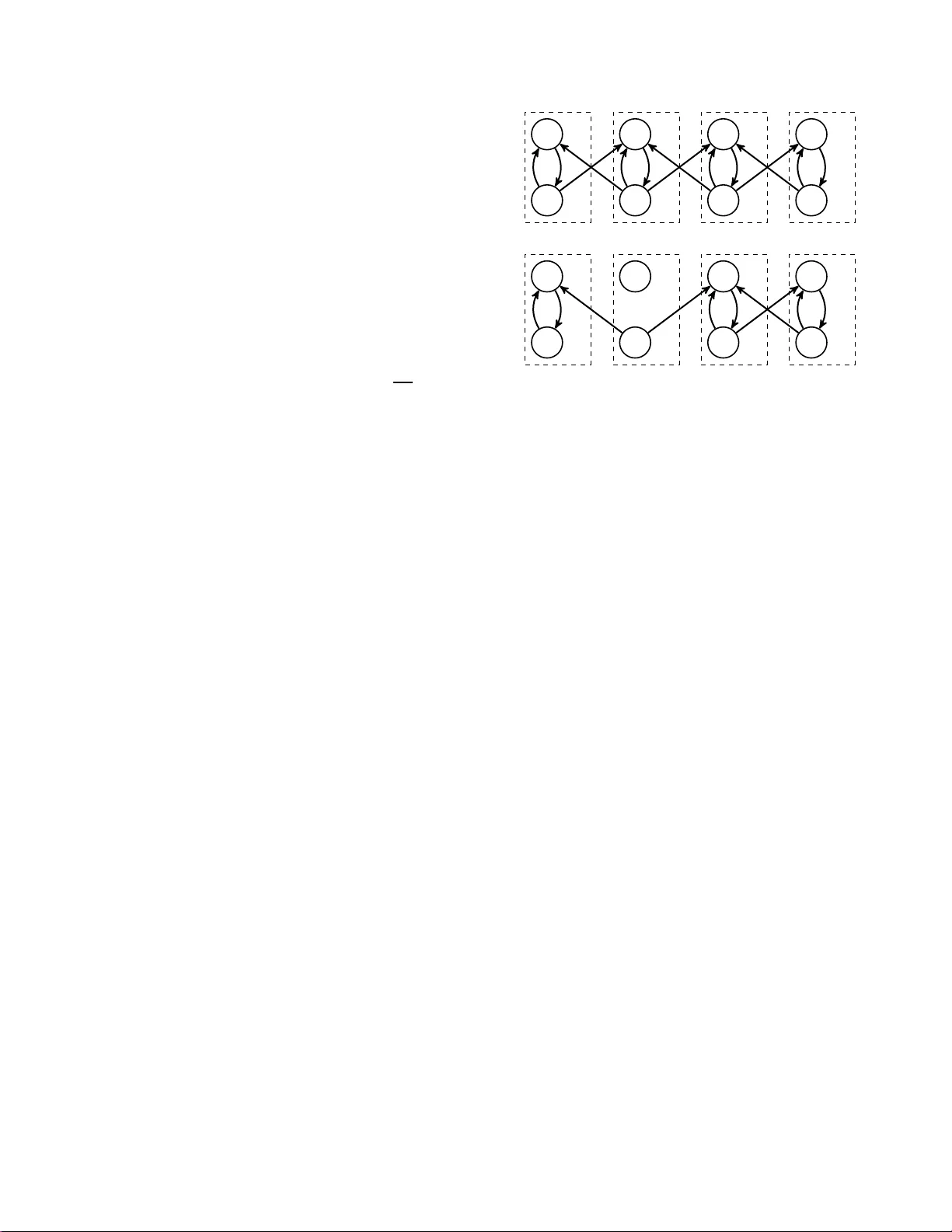
F rom Ordinary Differen tial Equ ations to Structural Causal Mo dels: the deterministic case Joris M. Mo oij Institute for Computing and Information Sciences Radb oud Univ ersity Nij megen The Netherlands Dominik Janzing Max Planck Institute for Int elligent Systems T¨ ubingen, Germany Bernhard Sc h¨ olk opf Max Planck Institute for Int elligent Systems T¨ ubingen, Ger many Abstract W e s how how, and under whic h co nditions, the equilibr ium states of a first-or der Ordi- nary Different ial Eq uation (ODE) system can be describ ed with a deterministic Structural Causal Model (SCM). Our exp ositio n sheds more light on the concept of causality as ex- pressed within the framework of Structural Causal Mo dels, esp ecially for cyclic mo dels. 1 In tro duction Over t he last few decades, a compr e he ns ive t heory for acyclic causal models was developed (e.g., see (P earl, 2000; Spirtes et al., 199 3)). In particular, different, but related, approaches to causal inference and mod- eling have b een prop osed for the causa lly sufficien t case. These approaches are based on different start- ing points. One a pproach s tarts fr om the (lo ca l or global) causal Marko v conditio n and links obser ved in- depe ndence s to the ca usal graph. Another a pproach uses causal Bay es ia n netw orks to link a par ticular fac- torization of the joint distribution of the v aria bles to causal semantics. The third appr oach u ses a structural causal model (sometimes also called structural equa- tion mo del or functional caus al mo del) where each ef- fect is ex pr essed a s a function o f its direct ca uses and an uno bserved noise v ariable . The relationships b e- t ween these apr oaches are well understo o d (Lauritzen, 1996; Pearl, 200 0). Over the years, several attempts ha v e been made to extend the theory to the cyclic ca se, thereby enabling causal modeling of systems that inv olve feedbac k (Spirtes, 1 995; Koster, 1996; Pearl and Dech ter, 19 96; Neal, 2 000; Hyttinen et a l., 20 12). Ho w ever, the rela- tionships b etw een the different approaches mentioned befo re do no t immediately genera lize to the cyclic ca se in gener al (although partial r esults are kno wn for the linear case and the discrete case). Nev ertheless, several algorithms (starting from differe n t as sumptions) hav e bee n propose d for inferring cyclic causa l mo dels from observ ational data (Richardson, 1 9 96; La cerda e t al., 2008; Sc hmidt a nd Murph y, 2009; Itani et al., 2010; Mo oij et al., 201 1). The most stra ightforw ard extension to the cyclic ca s e seems to be offered by the structural causal model framework. Indeed, the for malism s tays intact when one s imply dro ps the a cyclicity constraint. How ever, the question then aris e s how to interpret cyclic struc- tural equatio ns. One option is to as sume an under - lying discrete-time dynamical system, in which the structural equations ar e used as fixed p oint equa- tions (Spirtes , 1995; Dash, 2005; Lacer da et al., 2 008; Mo oij et al., 20 1 1; Hyttinen et a l., 2012), i.e., they are used as up date rules to calculate the v alues at time t + 1 from the v alues at time t , and then one lets t → ∞ . Here we show how an alternative in- terpretation of structural causal mo dels aris e s natu- rally when considering systems of ordinar y differen- tial equations. B y considering how these differential equations b ehave in an equilibr ium state, we arrive at a str uctural causa l mo del that is time indep endent, yet where the causal sema ntics p ertaining to inter- ven tio ns is still v alid. As o pp o sed to the usual inter- pretation as discr e te- time fixed p oint eq uations, the contin uo us-time dynamics is no t defined by the struc- tural equations. Instead, we descr ib e ho w the struc- tural equatio ns arise fro m the given dynamics. Th us it becomes evident that different dynamics can yield ident ical str uctural causal mo dels . This interpretation sheds more light on the meaning of structural equa- tions, and do es no t make any substantial distinction betw een the cyclic and acyclic cas e s. It is sometimes ar gued that inferring causality amounts to simply inferring the time str ucture con- necting the obser ved v ariables, since the cause always preceeds the effect. This, ho w ever, ignor es tw o im- po rtant facts: First, time order b etw een tw o v ar iables do es not tell us whether the ear lier one caused the later one, or whether both ar e due to a common cause. This pap er addresses a second counter ar gument: a v ar iable need not nec e ssarily refer to a measur e men t p er formed at a cer tain time instance. Instead, a causal graph may formalize how intervening on so me v aria bles influences the equilibrium state o f other s . This describes a phe- nomenologica l lev el on whic h the original time struc- ture betw een v ariables g ets lost, but c a usal g raphs und structural equations ma y s till b e well-defined. On this level, also cyclic s tructural equations get a natural and well-defined meaning. F or simplicity , we consider o nly deterministic systems, and leave t he extension to sto chastic systems with po s- sible confounding as future work. 2 Ordinary Differen tial E quations Let I := { 1 , . . . , D } b e a n index set of v ar iable lab els. Consider v ar iables X i ∈ R i for i ∈ I , where R i ⊆ R d i . W e will us e nor mal font for a single v ar iable and bo ldface for a tuple of v ar ia bles X I ∈ Q i ∈ I R i . 2.1 Observ ational s ys te m Consider a dynamical system D describ ed by D cou- pled first-order ordinar y differen tial equatio ns and an initial condition X 0 ∈ R I : 1 ˙ X i ( t ) = f i ( X pa D ( i ) ) , X i (0) = ( X 0 ) i ∀ i ∈ I (1) Here, pa D ( i ) ⊆ I is the set of (indices of ) p ar ents 2 of v ar iable X i , and eac h f i : R pa D ( i ) → R i is a (suf- ficient ly smo oth) function. This dynamical s ystem is assumed to describ e the “natural” o r “ observ ational” state of the system, without an y in ter vention from outside. W e will assume that if j ∈ pa D ( i ), then f i depe nds on X j (in other words, f i should not b e co n- stant w he n v arying X j ). Slightly abus ing terminology , we will henceforth call such a dynamical sy s tem D an Ordinary Differential Eq uation (ODE). The structure of these differential equations can b e represented as a directed gra ph G D , with one no de for each v ariable and a directed edge fro m X i to X j if and only if ˙ X j depe nds on X i . 2.1.1 Example: the Lotk a-V olterra mo del The Lotk a- V olterra mo del (Murray , 2002) is a w ell- known mo del from p opulation biology , mo deling the m utual influence of the abundance of pre y X 1 ∈ [0 , ∞ ) (e.g., rabbits) and the abundance o f pr edators X 2 ∈ 1 W e write ˙ X := dX dt . 2 Note that X i can be a parent of itself. X 1 X 2 (a) G D X 1 X 2 (b) G D do( X 2 = ξ 2 ) Figure 1: (a) Graph of the Lotk a-V olterra mo del (2); (b) Graph of the same ODE after the interv en tion do( X 2 = ξ 2 ), corres po nding with (5). [0 , ∞ ) (e.g., wolves): ( ˙ X 1 = X 1 ( θ 11 − θ 12 X 2 ) ˙ X 2 = − X 2 ( θ 22 − θ 21 X 1 ) ( X 1 (0) = a X 2 (0) = b (2) with all parameters θ ij > 0 and initial condition sa tis- fying a ≥ 0 , b ≥ 0. The g raph of this system is depicted in Figure 1(a). 2.2 P erfect in terv en ti ons Interventions on the system D descr ib e d in (1) can b e mo deled in differen t ways. Here we will fo cus on “p er- fe ct” interventions : for a subset I ⊆ I of components, we force the v alue of X I to attain some v a lue ξ I ∈ R I . In particular , w e will assume that the interven tion is active from t = 0 to t = ∞ , and that its v a lue ξ I do es not change ov er time. Inspir ed by the do-op er ator in- tro duced b y P earl (20 00), w e will deno te this t yp e of int erven tion as do( X I = ξ I ). On the lev el of the ODE, there ar e man y w ays of re- alizing a given p erfect interven tion. One p ossible wa y is to a dd terms o f the for m κ ( ξ i − X i ) (with κ > 0 ) to the expressio n for ˙ X i , for a ll i ∈ I : ˙ X i ( t ) = ( f i ( X pa D ( i ) ) + κ ( ξ i − X i ) i ∈ I f i ( X pa D ( i ) ) i ∈ I \ I , X i (0) = ( X 0 ) i (3) This w o uld cor resp ond to extending the system b y comp onents which monitor the v alues of { X i } i ∈ I and exert nega tive feedbac k if they devia te fro m their tar- get v alues { ξ i } i ∈ I . Subsequen tly , we let κ → ∞ to consider the idealized situation in which the in terven- tion completely o verrides the other mechanisms that normally deter mine the v alue of X I . Assuming that the functions { f i } i ∈ I are b ounded, w e can let κ → ∞ and o btain the intervene d system D do( X I = ξ I ) : ˙ X i ( t ) = ( 0 i ∈ I f i ( X pa D ( i ) ) i ∈ I \ I , X i (0) = ( ξ i i ∈ I ( X 0 ) i i ∈ I \ I (4) A p erfect interv en tion ch anges the graph G D asso ci- ated to the ODE D by removing the incoming a rrows on the no des cor resp onding to the in tervened v a r i- ables { X i } i ∈ I . It also changes the parent sets of in ter- vened v ar iables: for each i ∈ I , pa D ( i ) is r eplaced b y pa D do( X I = ξ I ) ( i ) = ∅ . 2.2.1 Example: L otk a-V olterra mo del Let us return to the example in sec tio n 2.1.1. In this context, consider the p erfect in terven tion do( X 2 = ξ 2 ). This interv en tion c o uld b e r ealized by monitoring the abundance of wolv es v e r y precisely and making sure that the num b er eq ua ls the target v alue ξ 2 at all time (for example, by killing an exces s o f wolv es and in- tro ducing new wolves fro m some reser voir of w olves). This leads to the following intervened O DE: ( ˙ X 1 = X 1 ( θ 11 − θ 12 X 2 ) ˙ X 2 = 0 ( X 1 (0) = a X 2 (0) = ξ 2 (5) The co rresp onding intervened graph is illustrated in Figure 1(b). 2.3 Stability An imp o r tant concept in our context is stabi lity , de- fined as follows: Definition 1 The ODE D sp e cifie d in (1) is c al le d stable if t her e exists a unique e quilibrium state X ∗ ∈ R I such that for any initial state X 0 ∈ R I , the system c onver ges to this e quilibrium state as t → ∞ : ∃ ! X ∗ ∈R I ∀ X 0 ∈R I : lim t →∞ X ( t ) = X ∗ . One can weak en the stability condition by demanding conv ergence to and uniquenes s of the equilibrium o nly for a certain subset of a ll initial states. F or cla rity of exp osition, we will use this str ong sta bility co ndition. W e can extend this concept of stability by consider ing a certain set of p e rfect interv en tions: Definition 2 L et J ⊆ P ( I ) . 3 The OD E D sp e cifie d in (1) is c al le d s table with r esp ect to J if for al l I ∈ J and for al l ξ I ∈ R I , the intervene d ODE D do( X I = ξ I ) has a unique e quilibrium state X ∗ do( X I = ξ I ) ∈ R I such that fo r any initial state X 0 ∈ R I with ( X 0 ) I = ξ I , the system c onver ges to this e quilibrium a s t → ∞ : ∃ ! X ∗ do( X I = ξ I ) ∈R I ∀ X 0 ∈R I s.t. ( X 0 ) I = ξ I : lim t →∞ X ( t ) = X ∗ do( X I = ξ I ) . 3 F or a set A , w e denote with P ( A ) t he p ow er set of A (the set of all subsets of A ). This definition can also be w eakened by not demand- ing stabilit y for all ξ I ∈ R I , but for smaller subse ts instead. Again, we will use this strong condition f or clarity of expositio n, a lthough in a conc r ete example to be discussed la ter (see Section 2.3 .2), we will actually weak en the stability as sumption a long these lines. 2.3.1 Example: the Lotk a-V olterra m o del The ODE (2) of the Lotk a-V olterra model is not sta- ble, as discussed in detail b y Mur ray (2002). Indeed, it has tw o eq uilibrium states, ( X ∗ 1 , X ∗ 2 ) = (0 , 0) and ( X ∗ 1 , X ∗ 2 ) = ( θ 22 /θ 21 , θ 11 /θ 12 ). The J acobian of the dynamics is given by: ∇ f ( X ) =  θ 11 − θ 12 X 2 − θ 12 X 1 θ 21 X 2 − θ 22 + θ 21 X 1  In the first equilibrium state, it has a p o sitive and a negative eigen v alue ( θ 11 and − θ 22 , respectively), and hence this equilibrium is unstable. At the second eq ui- librium state, the Jaco bia n simplifies to  0 − θ 12 θ 22 /θ 21 θ 21 θ 11 /θ 12 0  which ha s tw o imaginary eigenv alues, ± i √ θ 11 θ 22 . One can s how (Murray, 200 2) that the steady state of the system is an undamped oscillation around this equi- librium. The in tervened system (5) is only gener ic ally stable, i.e., for most v alues o f ξ 2 : the unique stable eq uilib- rium state is ( X ∗ 1 , X ∗ 2 ) = (0 , ξ 2 ) as long as θ 11 − θ 12 ξ 2 6 = 0. If θ 11 − θ 12 ξ 2 = 0, there exis ts a fa mily of equilibria ( X ∗ 1 , X ∗ 2 ) = ( c, ξ 2 ) with c ≥ 0. 2.3.2 Example: da mp ed harmonic o s cillators The fav orite to y example of physicists is a system of coupled harmonic osc illa tors. Consider a o ne - dimensional system of D point mass es m i ( i = 1 , . . . , D ) with p ositions Q i ∈ R and momenta P i ∈ R , coupled by spr ings with spring constants k i and e q ui- librium le ngths l i , under influence of frictio n with fric- tion co e fficie n ts b i , with fixed end po sitions (see also Figure 2). W e first sketc h the qualitative b ehavior: there is a unique equilibr ium p ositio n where the s um of for ces v anishes f or ev ery single ma ss. Moving one or several m 1 m 2 m 3 m 4 k 0 k 1 k 2 k 3 k 4 Q = 0 Q = L Figure 2: Mass -spring system for D = 4. masses out o f their equilibr ium p o sition stimulates vi- brations of the entire system. Damp ed by friction, ev- ery mass conv erges to its unique and stable equilibrium po sition in the limit of infinite tim e. If one or several masses are fixed to p ositions differe n t from their eq ui- librium points, the po s itions of the r emaining masses still co nv e r ge to unique (but different) equilibrium po- sitions. The structur al eq uations that we derive later will descr ib e the change of the unconstra ined equilib- rium p ositions caused by fixing the others . The equations of motion for this system a re given by: ˙ P i = k i ( Q i +1 − Q i − l i ) − k i − 1 ( Q i − Q i − 1 − l i − 1 ) − b i m i P i ˙ Q i = P i /m i where w e define Q 0 := 0 and Q D +1 := L . The graph of this ODE is depicted in Figure 3(a). A t equilibrium (for t → ∞ ), all momenta v anish, and the follo wing equilibrium equations hold: 0 = k i ( Q i +1 − Q i − l i ) − k i − 1 ( Q i − Q i − 1 − l i − 1 ) 0 = P i which is a linear system of equations in terms of the Q i . There are D equations for D unknowns Q 1 , . . . , Q D , and one can easily c hec k that it has a unique solution. A p er fect interv en tion on Q i corres p o nds to fixat- ing the p osition of the i ’th mass. Physically , this is achiev ed b y adding a for ce that drives Q i to some fixed location, i.e., the in terven tio n on Q i is ac hieved through modifying the equation of motion for ˙ P i . T o deal with this example in o ur framework, we co nsider the pair s X i := ( Q i , P i ) ∈ R 2 to b e the element ary v aria bles. Consider for e x ample the p erfect interven- tion do( X 2 = ( ξ 2 , 0)), which effectively r eplaces the dynamical equations ˙ Q 2 and ˙ P 2 by ˙ Q 2 = 0, ˙ P 2 = 0 and their initial conditions b y ( Q 0 ) 2 = ξ 2 , ( P 0 ) 2 = 0. The g r aph of the corr esp onding ODE is depicted in Figure 3(b). Because of the fr iction, also this inter- vened system conv erges to a unique equilibrium that do es not dep end on the initial v a lue. This holds mo re generally : for any perfect in terven- tion o n (any n um b er) o f pairs X i of the t yp e do ( X i = ( ξ i , 0)), the interv ened system will conv erge tow ar ds a unique equilibrium b ecaus e of th e damping term. In- terven tions that result in a nonzero v alue for any mo- men tum P i while the corresp onding position is fixed are ph ysically imp ossible, and hence will not b e co nsid- ered. Concluding, we ha ve seen that the mass-spr ing system is sta ble with r esp ect to p erfect interven tio ns on an y num ber of p os ition v a riables, whic h we mo del mathematically as a joint interv en tion on the corre - sp onding pairs of po sition and momentum v a riables. Q 1 Q 2 Q 3 Q 4 P 1 P 2 P 3 P 4 X 1 X 2 X 3 X 4 (a) G D Q 1 Q 2 Q 3 Q 4 P 1 P 2 P 3 P 4 X 1 X 2 X 3 X 4 (b) G D do( Q 2 = ξ 2 ,P 2 =0) Figure 3: Graphs of the dynamics of the mass-spr ing system for D = 4. (a ) Observ a tional situation (b) Int erven tion do( Q 2 = ξ 2 , P 2 = 0). 3 Equilibrium equations In this section, w e will study how the dynamical equa - tions giv e rise to e quilibrium e quations that describe equilibrium states, and how these c ha nge under p erfect int erven tions. This is an intermediate r epresentation on o ur wa y to structural caus a l mo dels. 3.1 Observ ational s ys te m A t equilibrium, the rate of c hange o f an y v a riable is zero, by definition. Therefore, an e q uilibrium sta te of the obs erv atio na l system D defined in (1) satisfies the following e quilibri um e quations : 0 = f i ( X pa D ( i ) ) ∀ i ∈ I . (6) This is a set of D coupled equations with unkno wns X 1 , . . . , X D . The s ta bilit y assumption (cf. Defini- tion 1 ) implies tha t there exists a unique solution X ∗ of the equilibrium equations (6). 3.2 In terv ened systems Similarly , for the interv ened system D do( X i = ξ i ) defined in (4), we obtain the following equilibr ium equatio ns: ( 0 = X i − ξ i ∀ i ∈ I 0 = f j ( X pa D ( j ) ) ∀ j ∈ I \ I (7) If the system is stable with respec t to this interv en- tion (cf. Definition 2), then there exists a unique so- lution X ∗ do( X I = ξ I ) of the interv ened equilibrium equa- tions (7). Note that we c an als o g o directly from the equilib- rium equations (6) of the observ atio nal sy stem D to the equilibr ium eq uations (7) of the in tervened s y stem D do( X I = ξ I ) , simply by r eplacing the equilibr ium equa - tions “0 = f i ( X pa D ( i ) )” for i ∈ I b y equations of the form “0 = X i − ξ i ”. Indeed, note that the mo dified dynamical equation ˙ X i = f i ( X pa D ( i ) ) + κ ( ξ i − X i ) yields an equilibrium equation of the for m 0 = f i ( X pa D ( i ) ) + κ ( ξ i − X i ) which, in the limit κ → ∞ , reduces to 0 = X i − ξ i (assuming that f i is b ounded). This seemingly tr ivial observ ation will turn out to b e quite imp or tant. 3.3 Lab eling equili brium equations If we w ould c o nsider the equilibrium equations as a set of un lab ele d equations {E i : i ∈ I } , where E i de- notes the equilibrium equation “0 = f i ( X pa D ( i ) )” (or “0 = X i − ξ i ” after an interv en tion) for i ∈ I , then we will no t b e able to correctly predict the result of inter- ven tio ns , as we do not kno w which of the equilibr ium equations should be changed in order to model the particular interven tion. This information is pr e sent in the dynamical s ystem D (indeed, the terms “ ˙ X i ” in the l.h.s. of the dyna mical equations in (1) indica te the targ ets of the interv en tion), but is lost whe n con- sidering the corr esp onding equilibrium eq ua tions (6) as an unlab e led set (beca use the terms “ ˙ X i ” are a ll replaced by zero es). This imp ortant infor ma tion can b e preserved by la- beling the equilibrium equations. Indeed, the lab ele d set of equilibr ium equations E := { ( i, E i ) : i ∈ I } contains all information needed to predict how equi- librium states c hange o n arbitrary (perfect) in terven- tions. Under an in ter ven tion do( X I = ξ I ), the equi- librium equa tions are c hanged a s follows: for eac h in- tervened co mpo nent i ∈ I , the equilibrium eq ua tion E i is replaced by the eq uation ˜ E i defined as “0 = X i − ξ i ”, whereas the o ther equilibr ium equations E j for j ∈ I \ I do not c hange. Assuming that the dynamical system is stable with resp ect to this in ter ven tion, this mo di- fied s y stem of eq uilibrium e quations describ es the new equilibrium obtained under the interven tio n. W e con- clude tha t the information ab out the v alues of eq uilib- rium states and how these change under p erfect inter- ven tio ns is enco ded in the lab eled equilibrium equa- tions. 3.4 Lab eled equil ibrium equations The previous consider ations motiv ate the follo wing formal definition of a system of Lab eled Equilibrium Equations (LE E) and their semantics under in terven- tions. Definition 3 A system of Labeled Equilibr ium Equations (LEE) E for D variables { X i } i ∈I with I := { 1 , . . . , D } c onsists of D labeled equations of the form E i : 0 = g i ( X pa E ( i ) ) , i ∈ I , (8) wher e pa E ( i ) ⊆ I is the set of (indic es of ) parents of variable X i , and e ach g i : R pa E ( i ) → R i is a function. The st ructur e of an LEE E can b e repres ent ed as a directed gra ph G E , with one no de for ea ch v ariable and a directed e dg e from X i to X j (with j 6 = i ) if a nd only if E i depe nds on X j . A p erfect interven tion transforms an LEE in to a nother (in tervened) LEE: Definition 4 L et I ⊆ I and ξ I ∈ R I . F or the p erfe ct intervention do( X I = ξ I ) that for c es t he variables X I to take the value ξ I , the intervene d LEE E do( X I = ξ I ) is obtaine d by r eplaci ng the lab ele d e quations of t he origi - nal LEE E by the fol lowing mo difie d lab ele d e qu ations: 0 = ( X i − ξ i i ∈ I g i ( X pa E ( i ) ) i ∈ I \ I . (9) W e define the concept of solv ability for LEEs that mir- rors the definition of stability for ODE s: Definition 5 An LEE E is c al le d so lv able if ther e ex- ists a unique solution X ∗ to the system of (lab ele d) e quations {E i } . An LEE E is c al le d solv able with re- sp ect to J ⊆ P ( I ) if for al l I ∈ J and for al l ξ I ∈ R I , the i ntervene d LEE E do( X I = ξ I ) is s olvable. As we s aw in the pr e vious se c tion, a n O DE induces an LEE in a straig ht forward way . The graph G E D of the induced LEE E D is equal to the graph G D of the ODE D . It is immedia te that if the ODE D is stable, then the induced LEE E D is solv able. As we saw a t the end of Section 3.2, our ways of mo deling in terven tions on ODEs a nd on LEE s are compatible. W e will sp ell out this imp o rtant result in detail. Theorem 1 L et D b e an ODE, I ⊆ I and ξ I ∈ R I . (i) Applying the p erfe ct intervention do( X I = ξ I ) to the induc e d LEE E D gives the same r esult as c onst r u ct- ing the LEE c orr esp onding t o the intervene d ODE D do( X I = ξ I ) : ( E D ) do( X I = ξ I ) = E D do( X I = ξ I ) . (ii) Stability of the ODE D with r esp e ct to t he interven- tion do( X I = ξ I ) implies solvability of the induc e d in- tervene d LEE E D do( X I = ξ I ) , and the c orr esp onding e qui- librium and solution X ∗ do( X I = ξ I ) ar e identic al.  3.5 Example: damped harmonic o s cillators Consider aga in the example of the damp e d, coupled harmonic oscillator s of section 2.3.2. The lab eled eq ui- librium equations ar e given explicitly by: E i :      0 = k i ( Q i +1 − Q i − l i ) − k i − 1 ( Q i − Q i − 1 − l i − 1 ) 0 = P i (10) 4 Structural Causal Mo dels In this section we will show ho w an LEE representation can be mapped to the mor e p opular re presentation of Structural Causa l Mo dels, a lso known as Structural Equation Mo dels (Bollen, 1 989). W e fo llow the ter- minology o f P earl (2000), but c o nsider her e only the sub c lass of deterministic SCMs. 4.1 Observ ational The following definition is a specia l case o f the mor e general definition in (Pearl, 200 0, Section 1 .4.1): Definition 6 A deterministic Str uctural Causal Mo del (SCM) M on D variables { X i } i ∈I with I := { 1 , . . . , D } c onsists of D structural equations of the f orm X i = h i ( X pa M ( i ) ) , i ∈ I , (11) wher e pa M ( i ) ⊆ I \ { i } is the set of ( indic es of ) par- ent s of vari able X i , and e ach h i : R pa M ( i ) → R i is a function. Each structural equation con tains a function h i that depe nds o n the compo nents of X in pa M ( i ). W e think of the parents pa M ( i ) as the dir e ct c auses of X i (rel- ative to X I ) and the function h i as th e c ausal me ch- anism that maps the direct causes to the effect X i . Note that the l.h.s. of a structura l equa tion by defini- tion contains only X i , a nd that the r.h.s. is a function of v ar iables excluding X i itself. In other w ords, X i is not considered to b e a direct cause of itself. The struc- tur e of an SCM M is often represented as a directed graph G M , with one no de for each v ariable and a di- rected edge fr om X i to X j (with j 6 = i ) if and only if h i depe nds o n X j . Note that this g raph do es not contain “self-lo ops” (edge s p o inting fro m a no de to itself ), by definition. 4.2 In terv entions A Structural Causal Model M comes with a s p ecific semantics for mo deling perfect in terv entions (Pearl, 2000): Definition 7 L et I ⊆ I and ξ I ∈ R I . F or the p erfe ct intervention do( X I = ξ I ) that for c es t he variables X I to take the value ξ I , t he int ervene d SCM M do( X I = ξ I ) is obtaine d by r eplaci ng the stru ct ur al e quations of the original SCM M by the fol lowing mo difie d structur al e quations: X i = ( ξ i i ∈ I h i ( X pa M ( i ) ) i ∈ I \ I . (12) The rea son that the equatio ns in a SCM ar e called “structural equations” (instead of simply “equations”) is that they also contain information for mo deling in- terven tions, in a similar w ay as the la be le d equilibr ium equations con tain this information. In particular, the l.h.s. of the structural equations indicate the targets of an interv en tion. 4 4.3 Solv abili t y Similarly to our definition for LEEs , we define: Definition 8 An SCM M is c al le d solv able i f ther e exists a unique solut ion X ∗ to the system of struct ur al e quations. An SCM M is c al le d solv able w ith resp ect to J ⊆ P ( I ) if fo r al l I ∈ J and for al l ξ I ∈ R I , the intervene d SCM M do( X I = ξ I ) is s olvable. Note that each (deterministic) SCM M with acyclic graph G M is solv able, even with respect to the set of all p ossible interven tion targ e ts, P ( I ). T his is no t necessarily true if directed cycles ar e pr esent. 4.4 F rom lab el ed equilibrium equations to deterministi c SCMs Finally , w e will no w s how that under certain stability assumptions o n an ODE D , w e can r epresent the in- formation ab out (in ter vened) equilibrium states that is contained in the corresp onding set of lab eled equi- librium equations E D as an SCM M E D . First, given an L E E E , we will construct an induced SCM M E , pr ovided certain solv ability conditions hold: Definition 9 If for e ach i ∈ I , the LEE E is solvable with r esp e ct to some I i ⊆ I with pa E ( i ) \ { i } ⊆ I i ⊆ I \ { i } , then it is c al le d str uc tur ally so lv able . 4 In P earl (2000)’s words: “Mathematically , the distinc- tion b etw een stru ctural and algebraic equations is that the latter are c haracterized b y the set of solutions to the entire system of equ ations, whereas the former are characterized by th e solutions of eac h individu al equation. The implica- tion is that any subset of structural equ ations is, in itself, a v alid model of realit y—one t hat prev ails under some set of interv entions.” If the LEE E is structurally solv able, we can pro cee d as follows. Let i ∈ I . W e define the induced parent set pa M E ( i ) := pa E ( i ) \ { i } . Assuming structural s o lv abil- it y of E , under the p erfect interven tion do( X I i = ξ I i ), there is a unique solutio n X ∗ do( X I i = ξ I i ) to the in ter- vened LEE , for an y v alue of ξ I i ∈ R I i . This defines a function h i : R pa M E ( i ) → R i given b y the i ’th comp o- nent h i ( ξ pa M E ( i ) ) :=  X ∗ do( X I i = ξ I i )  i . The i ’th struc- tural equation of the induced SCM M E is defined as: X i = h i ( X pa M E ( i ) ) . Note that this equa tion is e quivalent to the lab eled equation E i in the se nse that they hav e identical solu- tion sets { ( X ∗ i , X ∗ pa M E ( i ) ) } . Repeating this pro cedure for all i ∈ I , we obtain the induced SCM M E . This construction is designed to preser ve the impo r- tant mathematical structure. In particular : Lemma 1 L et E b e an LEE, I ⊆ I and ξ I ∈ R I and c onsider the p erfe ct intervention do( X I = ξ I ) . Supp ose that b oth the LEE E and the intervene d LEE E do( X I = ξ I ) ar e structur al ly solvab le. (i) Applying the intervention do( X I = ξ I ) t o the induc e d SCM M E gives the same r esu lt as c onstructing the SCM c orr e- sp onding to the intervene d LEE E do( X I = ξ I ) : ( M E ) do( X I = ξ I ) = M E do( X I = ξ I ) . (ii) Solvabil ity of the LEE E with r esp e ct to the in- tervention do( X I = ξ I ) implies solvability of the induc e d SCM M E with r esp e ct to the same inter- vention do( X I = ξ I ) , and their r esp e ctive solutions X ∗ do( X I = ξ I ) ar e identic al. Pro of. The first statemen t direc tly follows from the construction o f the induced SCM. The k ey observ a- tion rega rding solv ability is the following. F ro m the construction ab ov e it directly follows that ∀ X pa E ( i ) ∈R pa E ( i ) : 0 = g i ( X pa E ( i ) ) ⇐ ⇒ X i = h i ( X pa E ( i ) \{ i } ) . This trivially implies that ∀ X ∈R I : 0 = g i ( X pa E ( i ) ) ⇐ ⇒ X i = h i ( X pa M E ( i ) ) . This implies that each simultaneous solutio n of a ll la - bele d equations is a simultaneous solution of a ll struc- tural equations, and vice versa: ∀ X ∈R I :   ∀ i ∈I : 0 = g i ( X pa E ( i ) )  ⇐ ⇒  ∀ i ∈I : X i = h i ( X pa M E ( i ) )   . The crucial p oint is that this still holds if an interv en- tion replaces some of the equations (b y 0 = X i − ξ i and X i = ξ i , r esp ectively , for all i ∈ I ).  4.5 F rom ODEs to determi nistic SCMs W e can now combine all the results a nd definitions s o far to construct a deterministic SCM fr om an ODE under c ertain stability conditio ns . W e define: Definition 10 An ODE D is c al le d s tructurally sta- ble if for e ach i ∈ I , the ODE D is stable with r esp e ct to some I i ⊆ I with pa D ( i ) \ { i } ⊆ I i ⊆ I \ { i } . Consider the diagram in Figure 4. Here, the lab els of the arrows corres p o nd with the num b ers of the sec- tions that discuss the co rresp onding mapping. The down ward mappings co rresp ond with a particular in- terven tion do( X I = ξ I ), applied at the differe n t levels (ODE, induced LE E, induced SCM). O ur main result: Theorem 2 If b oth the ODE D and the intervene d ODE D do( X I = ξ I ) ar e structu ra l ly stable, then: (i) The diagr am in Figur e 4 c ommu tes. 5 (ii) If furthermor e, the ODE D is stable with r esp e ct to the intervention do( X I = ξ I ) , the SCM M E D do( X I = ξ I ) has a unique solution that c oincides with t he stable e quilibrium of the i ntervene d ODE D do( X I = ξ I ) . Pro of. Immediate from Theorem 1 and Lemma 1.  Note that even thoug h th e ODE may co ntain self- lo ops (i.e., the time der iv ative ˙ X i could dep end on X i itself, and hence i ∈ pa D ( i )), the induced SCM M E D do es not con tain self-lo ops b y constr uction (i.e., i 6∈ pa M E D ( i )). Somewhat surpris ingly , the structural stability conditions actually imply the exis tence of self- lo ops (b ecause if X i would not occur in the equilibrium equation ( E D ) i , its v a lue w ould b e undetermined and hence the equilibrium would not b e unique). Whether o ne prefers the SCM representation ov er the LEE representation is mainly a matter of pr actical con- siderations: both representations cont ain all the neces - sary informa tion to predict the results of a rbitrary per - fect interven tions , and o ne can easily go from the LEE representation to the SCM r e pr esentation. One can also easily go in the opposite direction, but this can- not b e done in a uniq ue wa y . F or exa mple, one co uld rewrite ea ch str uctur al equation X i = h i ( X pa M ( i ) ) as the equilibrium equation 0 = h i ( X pa M ( i ) ) − X i , but also a s the equilibrium equation 0 = h 3 i ( X pa M ( i ) ) − X 3 i (in bo th cases, it would b e given the la be l i ). In cas e the dynamics contains no directed cycles (not considering se lf-lo ops), the a dv ant age of the SCM rep- resentation is that it is more explicit. Star ting at 5 This means that it does not matter in whic h d irection one follo ws the arrows , the end result will b e the same. ODE D LEE E D SCM M E D 3.3 4.4 int ervened ODE D do( X I = ξ I ) int ervened LEE E D do( X I = ξ I ) int ervened SCM M E D do( X I = ξ I ) 3.3 4.4 2.2 3.2 4.2 Figure 4: Each of the arrows in the diagram corresp onds with a mapping that is desc r ib ed in the section that the lab el r efers to. The dashed ar rows are only defined under structural solv abilit y a ssumptions on the L E E. If the ODE D and intervened ODE D do( X I = ξ I ) are structurally stable, this diagr am c o mmu tes (cf. Theorem 2). the v ariables without par ent s, and following the top o- logical o rdering of the corres po nding directed a cyclic graph, we directly obtain the solution of an SCM by simple substitution in a finite num ber o f steps. On the other hand, the LEE representation is more implicit, and we need to so lve a set of equations. In the c y clic case, one ne e ds to s olve a set o f equa tions in b o th rep- resentations, and the difference is merely cosmetical. How ever, one could argue that the LEE representation is sligh tly mor e natur al in the cyclic case, as it do es not for ce us to mak e additional (structural) stability assumptions. 4.6 Example: damped harmonic o s cillators Figure 5 shows the gr aph o f the structura l causa l mo del induced by our co ns truction. It r eflects the int uition that at equilibrium, (the p osition of ) each mass has a dir e c t causa l influence o n (the p o sitions of ) its neighbors. Observing that the moment um v ari- ables alw ays v anish at equilibrium (even for a n y per- fect interven tion that we consider), w e can decide that the only relev ant v ar iables for the SCM are the p o si- tion v ar iables Q i . Then, we end up with the following structural equations: Q i = k i ( Q i +1 − l i ) + k i − 1 ( Q i − 1 + l i − 1 ) k i + k i +1 . (13) 5 Discussion In many empirical sciences (ph ys ics, chemistry , bio l- ogy , etc.) and in engineer ing, differential equa tio ns are a commonly us e d mo deling to ol. When estimating system characteristics from data, they are esp ecia lly X 1 X 2 X 3 X 4 Figure 5: Graph of the structural causal mo del in- duced by the mass-spr ing system for D = 4. useful if mea surements ca n be done o n the relev ant time scale. If equilibratio n time scales b ecome to o small with r esp ect to the temp or al resolution of mea- surements, ho wev er, the more natural representation may be in terms of structural ca usal mo dels. The main contribution o f this work is to build an explicit bridge from the w o rld of differe n tial equations to the world of ca usal mo dels. Our hop e is that this may aid in broadening the impact of causal mo deling. Note that informatio n is lost when g oing from a dy- namical system r epresentation to an equilibrium repre- sentation (either LEE or SCM), in particular the rate of conv ergence to ward equilibrium. If time-series da ta is av aila ble, the most na tural representation may be the dynamical sy s tem representation. If o nly snapshot data or equilibrium data is av ailable, the dynamica l system representation can be c o nsidered to b e ov erly complicated, and o ne may use the LEE or SCM rep- resentation instead. W e ha ve shown o ne particula r wa y in whic h structur a l causal models can b e “der ived”. W e do not cla im that this is the o nly wa y: on the contrary , SCMs can prob- ably b e obtained in several other ways and from other representations as w ell. One issue that we have no t yet addr essed is that of c onstant s of motion . F or ex- ample, if we would no t fix the end p oints of the chain of harmonic os cillators, then the total moment um of the system would dep end on the initial condition, and therefore the dynamics would not be stable anymore according to the definition we hav e used here. W e belie ve that th ese and similar issues can proba bly be solved b y being more e xplicit ab o ut which v ariables in the dynamics will be c o me par t o f the structural caus a l mo del. W e plan to address this in future work. W e a ls o in tend to extend the basic fr amework de- scrib ed here tow ards the mo re genera l sto chastic ca se. Uncertaint y o r “noise” can enter in tw o differen t wa ys: via uncertaint y ab o ut certain (constant) parameter s of the different ial equations, a nd via latent v a riables. A complicating factor that has to be address e d then (whic h does not play a role in the deterministic case) is co nfounding. Ac knowledgements W e thank B r am Thijssen, T o m Claa ssen, T om Heskes and Tjeerd Dijkstra fo r stimu lating discussions. JM was supp or ted b y NW O, the Netherlands Org anization for Scientifi c Resear ch (VENI g rant 639.03 1 .036). References Bollen, K. A. (1989). St ructur al Equations with L a- tent V ariables . John Wiley & Sons. Dash, D. (2005). Restructuring dynamic causal sys- tems in e q uilibrium. In Pr o c e e dings of t he T enth In- ternational Workshop on A rtificial Intel ligenc e and Statistics (A IST A TS 200 5) . Hyttinen, A., Eb erhar dt, F., and Hoy e r, P . (2012 ). Learning linear cyclic causal models with la tent v ar i- ables. Journal for Machine L e arning R ese ar ch , 13:338 7343 9. Itani, S., O hannessian, M., Sachs, K., Nolan, G. P ., and Dahleh, M. A. (20 1 0). Structure learning in causal cyclic netw orks. In JMLR Workshop and Con- fer enc e Pr o c e e dings , volume 6 , pag e 1 6517 6. Koster, J . T. A. (199 6). Marko v prop erties of nonrecursive causal mo dels. Annals of S t atistics , 24(5):214 8–21 77. Lacerda, G., Spirtes, P ., Ra msey , J., and Hoy er, P . O . (2008). Discovering cyclic ca usal models by indep en- dent co mpo nent s ana lysis. In Pr o c e e dings of the 24th Confer enc e on U nc ert ainty in Artificial Intel ligenc e (UAI-2008) . Lauritzen, S. (19 96). Gr aphic al mo dels . Clar endon Press. Mo oij, J. M., Janzing, D., Heskes, T., and Sch¨ olk opf, B. (2011). O n causal discov ery with cyclic addi- tive noise mo dels. In Shaw e - T aylor, J., Zemel, R., Bartlett, P ., P ereira, F., and W einber ger, K., editors, A dvanc es in N eur al Informatio n Pr o c essing S ystems 24 (NIPS*2011) , pages 639– 647. Murray , J. (2 002). Mathematic al Biolo gy. I: A n Intr o duction . Springer, 3 edition. Neal, R. (2000). On deducing conditional indep en- dence fr o m d -separ ation in ca usal gr aphs with feed- back. Journal of Artifici al Intel ligenc e R ese ar ch , 12:87– 91. Pearl, J. (2000). Causality . Cambridge Universit y Press. Pearl, J. and Dech ter, R. (199 6). Identifying indepen- dence in causal graphs w ith feedback. In Pr o c e e dings of the Twelfth Annual C onfer enc e on Unc ertainty in Artificia l Intel ligenc e (UAI-96) , pages 420–4 26. Richardson, T. (1 996). A discov er y a lgorithm for directed cyclic graphs. In Pr o c e e dings of the Twelfth Confer enc e on U nc ert ainty in Artificial Intel ligenc e (UAI-1996) . Schm idt, M. and Murphy , K. (2 0 09). Mo deling dis- crete interv en tional data using dir ected cyclic graph- ical mo dels . In Pr o c e e dings of the 25th Annual Confer enc e on U nc ert ainty in Artificial Intel ligenc e (UAI-09) . Spirtes, P . (1995). Directed cyclic graphical repre- sentations of feedbac k mo dels. In Pr o c e e dings of the 11th Confer enc e on Unc ertainty in Artificial In t el li- genc e (UAI-95) , pag e 4 9149 9. Spirtes, P ., Glymo ur, C., and Scheines, R. (1993). Causation, pr e diction, and se ar ch . Springer-V er lag. (2nd editio n MIT Pr e s s 200 0).