Unsupervised Feature Learning for low-level Local Image Descriptors
Unsupervised feature learning has shown impressive results for a wide range of input modalities, in particular for object classification tasks in computer vision. Using a large amount of unlabeled data, unsupervised feature learning methods are utili…
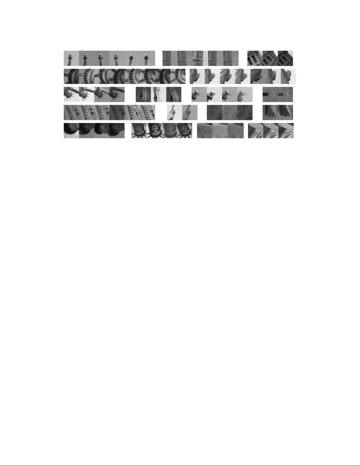
Authors: Christian Osendorfer, Justin Bayer, Sebastian Urban
Unsupervised F eatur e Lear ning f or low-lev el Local Image Descriptors Christian Osendorfer , Justin Bayer , Sebastian Urban, P atrick van der Smagt T echnische Universit ¨ at M ¨ unchen { osendorf, bayerj, surban, smagt } @in.tum.de Abstract Unsupervised feature learning has shown impressi ve results for a wide range of in- put modalities, in particular for object classification tasks in computer vision. Us- ing a large amount of unlabeled data, unsupervised feature learning methods are utilized to construct high-le vel representations that are discriminative enough for subsequently trained supervised classification algorithms. Howe ver , it has nev er been quantitatively in vestigated yet how well unsupervised learning methods can find low-level repr esentations for image patches without any additional supervi- sion. In this paper we examine the performance of pure unsupervised methods on a lo w-lev el correspondence task, a problem that is central to many Computer V i- sion applications. W e find that a special type of Restricted Boltzmann Machines (RBMs) performs comparably to hand-crafted descriptors. Additionally , a simple binarization scheme produces compact representations that perform better than sev eral state-of-the-art descriptors. 1 Introduction In this paper we tackle a recent computer vision dataset [2] from the viewpoint of unsupervised feature learning. Why yet another dataset? There are already enough datasets that serve well for ev aluating feature learning algorithms. In particular for feature learning from image data, several well-established benchmarks exist: Caltech-101 [10], CIF AR-10 [19], NORB [23], to name only a few . Notably , these benchmarks are all object classification tasks. Unsupervised learning algorithms are ev aluated by considering how well a subsequent supervised classification algorithm performs on high-level features that are found by aggregating the learned low-le vel representations [8]. W e think that mingling these steps makes it difficult to assess the quality of the unsupervised algorithms. A more direct way is needed to ev aluate these methods, preferably where a subsequent supervised learning step is completely optional. W e are not only at odds with the methodology of ev aluating unsupervised learning algorithms. Gen- eral object classification tasks are alw ays based on orientation- and scale-rectified pictures with objects or themes firmly centered in the middle. W e are looking for a dataset where it is possible to show that unsupervised feature learning is beneficial to the wide range of Computer V ision tasks beyond object classification, like tracking, stereo vision, panoramic stitching or structure from mo- tion. One might argue, that object classification acts as a good proxy for all these other tasks but this hypothesis has not shown to be correct either theoretically or through empirical evidence. In- stead, we chose the most general and direct task that can be be applied to low-le vel repr esentations : matching these representations, i.e. determining if two data samples are similar given their learned representation. Matching image descriptors is a central problem in Computer V ision, so hand-crafted descriptors are always e valuated with respect to this task [28]. Giv en a dataset of labeled correspondences, supervised learning approaches will find representations and the accompanying distance metric that 1 are optimized with respect to the induced similarity measure. It is remarkable that hand-engineered descriptors perform well under this task without the need to learn such a measure for their represen- tations in a supervised manner . T o the best of our knowledge it has nev er been in vestigated whether any of the many unsupervised learning algorithms developed over the last couple of years can match this performance without relying on any supervision signals. While we propose an additional benchmark for unsupervised learning algorithms, we do not introduce a ne w learning algorithm. W e rather in vestigate the per- formance of the Gaussian RBM (GRBM) [39], its sparse variant (spGRBM) [29] and the mean cov ariance RBM (mcRBM) [33] without any supervised learning with respect to the matching task. As it turns out, the mcRBM performs comparably to hand-engineered feature descriptors. In fact using a simple heuristic, the mcRBM produces a compact binary descriptor that performs better than sev eral state-of-the-art hand-crafted descriptors. W e begin with a brief description of the dataset used for ev aluating the matching task, followed by a section on details of the training procedure. In section 4 we present our results, both quantitativ ely and qualitati vely and also mention other models that were tested but not further analyzed because of overall bad performance. Section 5 concludes with a brief summary and an outlook for future work. A revie w of GRBMs, spGRBMs and mcRBMs is provided in the appendix, section 6, for completeness. Related work Most similar in spirit to our work are [6, 20, 22]: Like us, [6, 22] are interested in the behavior of unsupervised learning approaches without any supervised steps afterw ards. Whereas both inv estigate high-le vel representations. [20] learns a compact, binary representation with a very deep autoencoder in order to do fast content-based image search ( semantic hashing , [36]). Again, these representations are studied with respect to their capabilities to model high-lev el object concepts. Additionally , various algorithms to learn high-lev el correspondences hav e been studied [4, 37, 16] in recent years. Finding (compact) low-le vel image descriptors should be an excellent machine learning task: Even hand-designed des criptors ha ve man y free parameters that cannot (or should not) be optimized man- ually . Gi ven ground truth data for correspondences, the performance of supervised learning algo- rithms is impressiv e [2]. V ery recently , boosted learning with image gradient-based weak learners has sho wn excellent results [43, 42] on the same dataset used in this paper . See section 2 of [43] for more related work in the space of supervised metric learning. 2 Dataset At the heart of this paper is a recently introduced dataset for discriminati ve learning of local image descriptors [2]. It attempts to foster learning optimal low-le vel image representations using a large and realistic training set of patch correspondences. The dataset is based on more than 1.5 million image patches ( 64 × 64 pixels) of three different scenes: the Statue of Liberty (about 450,000 patches), Notre Dame (about 450,000 patches) and Y osemite’ s Half Dome (about 650,000 patches). The patches are sampled around interest points detected by Difference of Gaussians [27] and are normalized with respect to scale and orientation 1 . As shown in Figure 1, the dataset has a wide variation in lighting conditions, vie wpoints, and scales. The dataset contains also approximately 2.5 million image correspondences. Correspondences be- tween image patches are established via dense surface models obtained from stereo matching (stereo matching, with its epipolar and multi-view constraints, is a much easier problem than unconstrained 2D feature matching). The exact procedure to establish correspondences is more in volv ed and de- scribed in detail in [2, Section II]. Because actual 3D correspondences are used, the identified 2D patch correspondences show substantial perspectiv e distortions resulting in a much more realistic dataset than pre vious approaches [24, 28]. The dataset appears very similar to an earlier benchmark of the same authors [47], yet the correspondences in the nov el dataset resemble a much harder prob- lem. The error rate at 95% detection of correct matches for the SIFT descriptor [27] raises from 6% to 26%, the error rate for ev aluating patch similarity in pixel space (using normalized sum squared differences) raises from 20% to at least 48% (all numbers are take from [47] and [2] respectively), 1 A similar dataset of patches centered on multi-scale Harris corners is also av ailable. 2 Figure 1: Patch correspondences from the Liberty dataset. Note the wide v ariation in lighting, viewpoint and le vel of detail. The patches are centered on interest points but otherwise can be considered random, e.g. there is no reasonable notion of an object boundary possible. Figure taken from [2]. for example. In order to facilitate comparison of various descriptor algorithms a large set of prede- termined match/non-match patch pairs is provided. For ev ery scene, sets comprising between 500 and 500,000 pairs (with 50% matching and 50% non-matching pairs) are av ailable. W e don’t argue that this dataset subsumes or substitutes any of the pre viously mentioned bench- marks. Instead, we think that it can serve to complement those. It constitutes an excellent testbed for unsupervised learning algorithms: Experiments considering self-taught learning [32], effects of semi-supervised learning, supervised transfer learning over input distributions with a varying de- gree of similarity (the scenes of Statue of Liberty and Notredame show architectural structures, while Half Dome resembles a typical natural scenery) and the effect of enhancing the dataset with arbitrary image patches around ke ypoints can all be conducted in a controlled environment. Further- more, end-to-end trained systems for (large) classification problems (like [21, 5]) can be ev aluated with respect to this type of data distribution and task. 3 T raining Setup Different to [2], our models are trained in an unsupervised fashion on the a vailable patches. W e train on one scene (400,000 randomly selected patches from this scene) and ev aluate the performance on the test set of ev ery scene. This allo ws us to in vestigate the self-taught learning paradigm [32]. W e also train on all three scenes jointly (represented by 1.2 million image patches) and then ev aluate again e very scene indi vidually . 3.1 GRBM/spGRBM The GRBM and spGRBM (see Appendix, section 6.2) only differ in the setting of the sparsity penalty λ sp , all other settings are the same. W e use CD 1 [13] to compute the approximate gradient of the log-likelihood and the recently proposed rmsprop [41] method as gradient ascent method. Compared to standard minibatch gradient ascent, we find that rmsprop is a more efficient method with respect to the training time necessary to learn good representations: it takes at most half of the training time necessary for standard minibatch gradient ascent. Before learning the parameters, we first scale all image patches to 16 × 16 pixels. Then we preprocess all training samples by subtracting the vectors’ mean and dividing by the standard deviation of its elements. This is a common practice for visual data and corresponds to local brightness and contrast normalization. [39, Section 2.2] giv es also a theoretical justification for why this preprocessing step is necessary to learn a reasonable precision matrix Λ . W e find that this is the only preprocessing scheme that allo ws GRBM and spGRBM to achiev e good results. In addition, it is important to learn 3 Λ —setting it to the identity matrix, a common practice [14], also produces dissatisfying error rates. Note that originally it was considered that learning Λ is mostly important when one wants to find a good density (i.e. generativ e) model of the data. Both GRBM and spGRBM have 512 hidden units. The elements of W are initialized according to N (0 , 0 . 1) , the biases are initialized to 0. rmsprop uses a learning rate of 0 . 001 , the decay factor is 0 . 9 , the minibatch size is 128. W e train both models for 10 epochs (this takes about 15 minutes on a consumer GPU for 400000 patches). For the spGRBM we use a sparsity target of ρ = 0 . 05 and a sparsity penalty of λ sp = 0 . 2 . spGRBM is very sensitiv e to settings of λ sp [38]—setting it too high results in dead representations (samples that have no acti ve hidden units) and the results deteriorate drastically . 3.2 mcRBM mcRBM (see Appendix, section 6.3) training is performed using the code from [33]. W e resam- ple the patches to 16 × 16 pixels. Then the samples are preprocessed by subtracting their mean (patchwise), followed by PCA whitening, which retains 99% of the variance. The overall training procedure (with stochastic gradient descent) is identical to the one described in [33, Section 4]. W e train all architectures for a total of 100 epochs, ho wev er updating P is only started after epoch 50. W e consider two different mcRBM architectures: The first has 256 mean units, 512 factors and 512 cov ariance units. P is not constrained by any fixed topography . W e denote this architec- ture by mcRBM (256 , 512 / 512) . The second architecture is concerned with learning more compact representations: It has 64 mean units, 576 factors and 64 cov ariance units. P is initialized with a two-dimensional topography that takes 5 × 5 neighborhoods of factors with a stride equal to 3. W e denote this model by mcRBM (64 , 576 / 64) . On a consumer grade GPU it takes 6 hours to train the first architecture on 400000 samples and 4 hours to train the second architecture on the same number of samples. 4 Results For the results presented in this section (T able 1) we follow the e valuation procedure of [2]: For ev ery scene (Liberty (denoted by L Y), Notredame (ND) and Half Dome (HD)), we use the labeled dataset with 100,000 image pairs to assess the quality of a trained model on this scene. In order to sav e space we do not present R OC curves and only show the results in terms of the 95% err or rate which is the percent of incorrect matches when 95% of the true matches are found: After computing the respective distances for all pairs in a test set, a threshold is determined such that 95% of all matching pairs hav e a distance below this threshold. Non-matching pairs with a distance below this threshold are considered incorrect matches. T able 1 consists of two subtables. T able 1a presents the error rates for GRBM, spGRBM and mcRBM when no limitations on the size of representations are placed. T able 1b only considers descriptors that have an overall small memory footprint. For GRBM and spGRBM we use the activ ations of the hidden units gi ven a preprocessed input patch v as descriptor D ( v ) (see eq. 5, section 6.1): D ( v ) = σ ( v T Λ 1 2 W + b ) For the mcRBM a descriptor is formed by using the acti vations of the latent covariance units alone , see eq. 8, section 6.3: D ( v ) = σ ( P T ( C T v ) 2 + c ) This is in accordance with manually designed descriptors. Many of these rely on distributions (i.e. histograms) of intensity gradients or edge directions [27, 28, 1], structural information which is encoded by the cov ariance units (see also [35, Section 2]) 2 . 4.1 Distance metrics As we explicitly refrain from learning a suitable (with respect to the correspondence task) distance metric with a supervised approach, we hav e to resort to standard distance measures. The Euclidean 2 Extending the descriptor with mean units degrades results. 4 T est set Method T raining set L Y ND HD SIFT – 28.1 20.9 24.7 L Y 47.6 33.5 41.4 GRBM ND 50.0 33.4 42.5 ( L 1 ` 1 ) HD 49.0 34.0 41.5 L Y/ND/HD 48.7 33.5 42.1 L Y 37.9 26.9 34.3 spGRBM ND 40.0 28.0 35.4 ( L 1 ` 1 ) HD 39.1 27.9 34.9 L Y/ND/HD 37.5 26.6 33.6 L Y 31.3 25.1 34.5 mcRBM ND 34.0 25.6 33.0 ( L 1 ` 2 ) HD 31.2 22.3 25.7 L Y/ND/HD 30.8 24.8 33.3 L Y 34.7 24.2 38.6 mcRBM ND 33.3 24.8 44.9 (JSD) HD 29.9 22.7 37.6 L Y/ND/HD 30.0 23.1 39.8 (a) T est set Method T raining set L Y ND HD SIFT – 31.7 22.8 25.6 BRIEF – 59.1 54.5 54.9 BRISK – 79.3 74.8 73.2 SURF – 54.0 45.5 43.5 L Y – 16.9 22.8 BinBoost ND 20.4 – 18.9 (8 bytes) HD 21.6 14.5 – L Y – 31.1 34.4 ITQ-SIFT ND 37.0 – 34.3 (8 bytes) HD 37.3 30.5 – L Y – 43.1 47.2 D-Brief ND 46.2 – 51.3 (4 bytes) HD 53.3 43.9 – L Y 36.2 39.9 64.9 mcRBM ND 46.2 34.5 56.1 (8 bytes) YM 43.4 37.4 53.0 L Y/ND/HD 40.5 36.6 55.4 (b) T able 1: Error rates, i.e. the percent of incorrect matches when 95% of the true matches are found. All numbers for GRBM, spGRBM and mcRBMs are gi ven within ± 0 . 5% . Every subtable, indicated by an entry in the Method column, denotes a descriptor algorithm. Descriptor algorithms that do not require learning (denoted by – in the column T raining set ) are represented by one line. The numbers in the columns labeled L Y , ND and HD are the error rates of a method on the respective test set for this scene. Supervised algorithms are not ev aluated (denoted by –) on the scene they are trained on. The T raining set L Y/ND/HD encompasses 1.2 million patches of all three scenes; this setting is only possible for unsupervised learning methods. (a) Error rates for sev eral unsupervised algorithms without restricting the size of the learned representation. GRBM, spGRBM and mcRBM learn descriptors of dimensionality 512. ( L 1 ` 1 ) denotes that the error rates for a method are with respect to ` 1 normalization of the descriptor under the L 1 distance. (b) Results for compact descriptors. BRIEF (32 bytes) [3] and BRISK (64 bytes) [25] are binary descriptors, SURF [1] is a real valued descriptor with 64 dimensions. BinBoost [42], ITQ-SIFT [12] and D-Brief [44] learn compact binary descriptors with supervision. Numbers for BRIEF , BRISK, SURF , BinBoost and ITQ-SIFT are from [42]. distance is widely used when comparing image descriptors. Y et, considering the generativ e nature of our models we follow the general argumentation of [17] and choose the Manhattan distance, denoted in this text by L 1 . W e also consider two normalization schemes for patch representations, ` 1 and ` 2 (i.e. after a feature vector x is computed, its length is normalized such that k x k 1 = 1 or k x k 2 = 1 ). Giv en a visible input both (sp)GRBM and mcRBM compute features that resemble parameters of (conditionally) independent Bernoulli random v ariables. Therefore we consider the Jensen-Shannon div ergence (JSD) [26] as an alternative similarity measure. Finally , for binary descriptors, we use the Hamming distance. 4.2 SIFT Baseline SIFT [27] (both as interest point detector and descriptor) was a landmark for image feature matching. Because of its good performance it is one of the most important basic ingredients for man y dif ferent kinds of Computer V ision algorithms. It serves as a baseline for ev aluating our models. W e use vlfeat [45] to compute the SIFT descriptors. 5 The performance of the SIFT descriptor , ` 1 -normalized, is reported (using L 1 distance) in T able 1a, first entry . ` 1 normalization provides better results than ` 2 normalization or no normalization at all. SIFT performs descriptor sampling at a certain scale relativ e to the Difference of Gaussians peak. In order to achiev e good results, it is essential to optimize this scale parameter [2, Figure 6] on ev ery dataset. T able 1b is concerned with ev aluating compact descriptors: the first entry shows the performance of SIFT when used as a 128-byte descriptor (i.e. no normalization applied, but again optimized for the best scale parameter) with L 1 distance. 4.3 Quantitative analysis T able 1a shows that SIFT performs better than all three unsupervised methods. mcRBM (256, 512/512) performs similar to SIFT when trained on Half Dome, albeit at the cost of a 4.5 times larger descriptor representation. The compact binary descriptor (the simple binarization scheme is described below) based on mcRBM (64, 576/64) performs remarkably well, comparable or ev en better than sev eral state-of-the-art descriptors (either manually designed or trained in a supervised manner), see T able 1b, last entry . W e discuss in more detail sev eral aspects of the results in the following paragraphs. GRBM and spGRBM spGRBM performs considerably better than its non-sparse version (see T able 1a, second and third entries). This is not necessarily expected: Unlike e.g. in classification [8] sparse representations are considered problematic with respect to ev aluating distances directly . Lifetime sparsity may be after all beneficial in this setting compared to strictly enforced population sparsity . W e plan to in vestigate this issue in more detail in future work by comparing spGRBM to Cardinality restricted boltzman machines [38] on this dataset. Self-taught paradigm W e would expect that the performance of a model trained on the Liberty dataset and ev aluated on the Notre Dame scene (and vice versa) should be noticeably better than the performance of a model trained on Half Dome and ev aluated on the two architectural datasets. Howe ver , this is not what we observe. In particular for the mcRBM (both architectures) it is the opposite: T raining on the natural scene data leads to much better performance than the assumed optimal setting. Jensen-Shannon Div ergence Both GRBM and spGRBM perform poorly under the Jensen- Shannon diver gence similarity (ov erall error rates are around 60%), therefore we don’t report these numbers in the table. Similar , results for mcRBM under JSD are equally bad. Howe ver , if one scales down P by a constant (we found the v alue of 3 appropriat e), the results with respect to JSD improv e noticeably , see T able 1a, the last entry . The performance on the Half Dome dataset is still not good – the scaling factor should be learned [9], which we also plan for future work. Compact binary descriptor W e were not successful in finding a good compact representa- tion with either GRBM or spGRBM. Finding compact representations for any kind of input data should be done with multiple layers of nonlinearities [20]. But ev en with only two layers ( mcRBM (64 , 576 / 64) ) we learn relativ ely good compact descriptors. If features are binarized, the representation can be made ev en more compact (64 bits, i.e. 8 bytes). In order to find a suitable binarization threshold we employ the following simple heuristic: After training on a dataset is fin- ished we histogram all activations (v alues between 0 and 1) of the training set and use the median of this histogram as the threshold. 4.4 Qualitative analysis W e briefly comment on the developed filters (Figure 2). Unsurprisingly , spGRBM (Figure 2a) and mcRBM (Figure 2b—these are columns from C ) learn Gabor like filters. At a closer look we make some interesting observ ations: Figure 2c sho ws the diagonal elements of Λ 1 / 2 from a spGRBM. When computing a latent representation, the input v is scaled (elementwise) by this matrix, which, visualized as a 2D image, resembles a Gaussian that is dented at the center , the location of the keypoint of ev ery image patch. The mcRBM also builds filters around the keypoint: Figure 2d sho ws some unusual filters from C . They are centered around the keypoint and bear a strong resemblance to discriminati ve projections (Figure 2e) that are learned in a supervised way on this dataset [2, 6 (a) (b) (c) (d) (e) (f) Figure 2: (a) T ypical filters learned with spGRBM. (b) Filters from an mcRBM. (c) The pixelwise in verted standard deviations learned with a spGRBM plotted as a 2D image (darker gray intensities resemble lo wer numerical values). An input patch is elementwise multiplied with this image when computing the latent representation. This figure is generated by training on 32 × 32 patches for better visibility , but the same qualitativ e results appear with 16 × 16 patches. (d) The mcRBM also learns some variants of log-polar filters centered around the DoG keypoint. These are very similar to filters found when optimizing for the correspondence problem in a supervised setting. Sev eral of such filters are shown in subfigure (e), taken from [2, Figure 5]. Finally (f), the basic keypoint filters are combined with Garbor filters, if these are placed close to the center; the Garbor filters get systematically arranged around the keypoint filters. Figure 5]. Qualitativ ely , the filters in Figure 2d resemble log-polar filters that are used in several state-of-the-art feature designs [28]. The very focused keypoint filters (first column in Figure 2d) are often combined with Gabor filters placed in the vicinity of the center – the Garbor filters appear on their o wn, if they are too far from the center . If an mcRBM is trained with a fix ed topography for P , one sees that the Gabor filters get systematically arranged around the keypoint (Figure 2f). 4.5 Other models W e also trained se veral other unsupervised feature learning models: GRBM with nonlinear rectified hidden units 3 [30], various kinds of autoencoders (sparse [7] and denoising [46] autoencoders), K- 3 Our experiments indicate that rmsprop is in this case also beneficial with respect to the final results: It learns models that perform about 2-3% better than those trained with stochastic gradient descent. 7 means [7] and tw o layer models (stacked RBMs, autoencoders with two hidden layers, cRBM [34]). None of these models performed as good as the spGRBM. 5 Conclusion W e start this paper suggesting that unsupervised feature learning should be ev aluated (i) without us- ing subsequent supervised algorithms and (ii) more directly with respect to its capacity to find good low-le vel image descriptors. A recently introduced dataset for discriminati vely learning low-le vel local image descriptors is then proposed as a suitable benchmark for such an e valuation scheme that complements nicely the existing benchmarks. W e demonstrate that an mcRBM learns real-v alued and binary descriptors that perform comparably or e ven better to se veral state-of-the-art methods on this dataset. In future work we plan to evaluate deeper architectures [20], combined with sparse con volutional features [18] on this dataset. Moreo ver , ongoing work inv estigates sev eral algorithms [4, 37] for supervised correspondence learning on the presented dataset. References [1] H. Bay , T . T uytelaars, and L. V an Gool. Surf: Speeded up robust features. In Proc. ECCV , 2006. [2] M. Bro wn, G. Hua, and S. W inder . Discriminativ e learning of local image descriptors. IEEE P AMI , 2010. [3] M. Calonder, V . Lepetit, M. Ozuysal, T . Trzcinski, C. Strecha, and P . Fua. Brief: Computing a local binary descriptor very f ast. P attern Analysis and Machine Intelligence, IEEE T ransactions on , 34(7):1281–1298, 2012. [4] S. Chopra, R. Hadsell, and Y . LeCun. Learning a similarity metric discriminativ ely , with application to face verification. In Proc. CVPR , 2005. [5] D. Ciresan, U. Meier, and J. Schmidhuber . Multi-column deep neural networks for image classification. In Pr oc. CVPR , 2012. [6] A. Coates, A. Karpathy , and A. Ng. Emergence of object-selectiv e features in unsupervised feature learning. In Pr oc. NIPS , 2012. [7] A. Coates, H. Lee, and A. Ng. An analysis of single-layer networks in unsupervised feature learning. In Pr oc. AISTA TS , 2011. [8] A. Coates and A. Ng. The importance of encoding versus training with sparse coding and vector quanti- zation. In Pr oc. ICML , 2011. [9] G. Dahl, M. Ranzato, A. Mohamed, and G. Hinton. Phone recognition with the mean-cov ariance restricted boltzmann machine. In Pr oc. NIPS , 2010. [10] L. Fei-Fei, R. Fergus, and P . Perona. Learning generativ e visual models from few training examples: An incremental bayesian approach tested on 101 object categories. Computer V ision and Image Understand- ing , 2007. [11] Y . Freund and D. Haussler . Unsupervised learning of distributions on binary vectors using two layer networks. T echnical report, Uni versity of California, Santa Cruz, 1994. [12] Y . Gong, S. Lazebnik, A. Gordo, and F . Perronnin. Iterative quantization: A procrustean approach to learning binary codes for large-scale image retrie val. P attern Analysis and Machine Intelligence , 2012. [13] G. Hinton. Training products of experts by minimizing contrastiv e diver gence. Neural Computation , 14(8):1771–1800, 2002. [14] G. Hinton. A practical guide to training restricted boltzmann machines. T echnical report, Uni versity of T oronto, 2010. [15] G. Hinton and R. Salakhutdinov . Reducing the dimensionality of data with neural networks. Science , 313(5786):504–507, 2006. [16] G. Huang, M. Mattar, H. Lee, and E. Learned-Miller . Learning to align from scratch. In Pr oc. NIPS , 2012. [17] Y . Jia and T . Darrell. Heavy-tailed distances for gradient based image descriptors. In Pr oc. NIPS , 2011. [18] K. Kavukcuoglu, P . Sermanet, Y . Boureau, K. Gre gor , M. Mathieu, and Y . LeCun. Learning con v olutional feature hierarchies for visual recognition. In Pr oc. NIPS , 2010. [19] A. Krizhevsky . Learning multiple layers of features from tiny images. T echnical report, University of T oronto, 2009. 8 [20] A. Krizhevsky and G. Hinton. Using very deep autoencoders for content-based image retrieval. In Pr oc. ESANN , 2011. [21] A. Krizhevsky , I. Sutskev er , and G. Hinton. Imagenet classification with deep con volutional neural net- works. In Pr oc. NIPS , 2012. [22] Q. Le, R. Monga, M. Devin, G. Corrado, K. Chen, M. Ranzato, J. Dean, and A. Ng. Building high-level features using large scale unsupervised learning. In Pr oc. ICML , 2012. [23] Y . LeCun, F . Huang, and L. Bottou. Learning methods for generic object recognition with inv ariance to pose and lighting. In Pr oc. CVPR , 2004. [24] V . Lepetit and P . Fua. Keypoint recognition using randomized trees. IEEE P AMI , 28(9):1465–1479, 2006. [25] S. Leutenegger , M. Chli, and R. Siegwart. Brisk: Binary robust inv ariant scalable keypoints. In Pr oc. ICCV , 2011. [26] J. Lin. Di vergence measures based on the shannon entropy . Information Theory , IEEE T ransactions on , 37(1):145–151, 1991. [27] D. Lowe. Distincti ve image features from scale-inv ariant keypoints. International Journal of Computer V ision , 60(2):91–110, 2004. [28] K. Mikolajczyk and C. Schmid. A performance ev aluation of local descriptors. IEEE P AMI , 2005. [29] V . Nair and G. Hinton. 3-d object recognition with deep belief nets. In Pr oc. NIPS , 2009. [30] V . Nair and G. Hinton. Rectified linear units improve restricted boltzmann machines. In Pr oc. ICML , 2010. [31] R. Neal. Probabilistic inference using markov chain monte carlo methods. T echnical report, Univ ersity of T oronto, 1993. [32] R. Raina, A. Battle, H. Lee, B. Packer , and A. Ng. Self-taught learning: Transfer learning from unlabeled data. In Pr oc. ICML , 2007. [33] M. Ranzato and G. Hinton. Modeling pix el means and cov ariances using f actorized third-order boltzmann machines. In Pr oc. CVPR , 2010. [34] M. Ranzato, A. Krizhevsky , and G. Hinton. Factored 3-way restricted boltzmann machines for modeling natural images. In Pr oc. AIST A TS , 2010. [35] M. Ranzato, V . Mnih, and G. Hinton. Generating more realistic images using gated mrf ’ s. In Pr oc. NIPS , 2010. [36] R. Salakhutdinov and G. Hinton. Semantic hashing. International Journal of Appr oximate Reasoning , 2008. [37] J. Susskind, R. Memise vic, G. Hinton, and M. Pollefeys. Modeling the joint density of two images under a variety of transformations. In Proc. CVPR , 2011. [38] K. Swersky , D. T arlo w , I. Sutskev er , R. Salakhutdinov , R. Zemel, and R. Adams. Cardinality restricted boltzmann machines. In Pr oc. NIPS , 2012. [39] Y . T ang and A. Mohamed. Multiresolution deep belief networks. In Pr oc. AIST A TS , 2012. [40] T . T ieleman. Training restricted boltzmann machines using approximations to the likelihood gradient. In Pr oc. ICML , 2008. [41] T . T ieleman and G. Hinton. Lecture 6.5 - rmsprop: Divide the gradient by a running a verage of its recent magnitude. COURSERA: Neural Networks for Machine Learning, 2012. [42] T . T rzcinski, M. Christoudias, P . Fua, and V . Lepetit. Boosting binary image descriptors. T echnical report, EPFL, 2012. [43] T . T rzcinski, M. Christoudias, V . Lepetit, and P . Fua. Learning image descriptors with the boosting-trick. In Pr oc. NIPS , 2012. [44] T . T rzcinski and V . Lepetit. Efficient discriminativ e projections for compact binary descriptors. In Pr oc. ECCV , 2012. [45] A. V edaldi and B. Fulkerson. Vlfeat: An open and portable library of computer vision algorithms. In Pr oceedings of the International Confer ence on Multimedia , 2010. [46] P . V incent, H. Larochelle, Y . Bengio, and P . Manzagol. Extracting and composing robust features with denoising autoencoders. In Pr oc. ICML , 2008. [47] S. W inder and M. Brown. Learning local image descriptors. In Proc. CVPR , 2007. 9 6 A ppendix 6.1 Gaussian-Binary Restricted Boltzmann Machine The Gaussian-Binary Restricted Boltzmann Machine (GRBM) is an e xtension of the Binary-Binary RBM [11] that can handle continuous data [15, 39]. It is a bipartite Markov Random Field ov er a set of visible units, v ∈ R N v , and a set of hidden units, h ∈ { 0 , 1 } N h . Every configuration of units v and units h is associated with an energy E ( v , h ) , defined as E ( v , h ; θ ) = 1 2 v T Λ v − v T Λ a − h T b − v T Λ W h (1) with θ = ( W ∈ R N v × N h , a ∈ R N v , b ∈ R N h , Λ ∈ R N v × N v ) , the model parameters. W rep- resents the visible-to-hidden symmetric interaction terms, a and b represent the visible and hidden biases respectively and Λ is the precision matrix of v , taken to be diagonal. E ( v , h ) induces a probability density function ov er v and h : p ( v , h ; θ ) = exp − E ( v , h ; θ ) Z ( θ ) (2) where Z ( θ ) is the normalization partition function, Z ( θ ) = R P h exp − E ( v , h ; θ ) d v . Learning the parameters θ is accomplished by gradient ascent in the log-likelihood of θ gi ven N i.i.d. training samples. The log-probability of one training sample is log p ( v ) = − 1 2 v T Λ v + v T Λ a + N h X j log 1 + exp N v X i v T i ( Λ 1 2 W ) ij + b j !! − Z ( θ ) (3) Evaluating Z ( θ ) is intractable, therefore algorithms like Contrastive Div ergence (CD) [13] or per- sistent CD (PCD) [40] are used to compute an approximation of the log-likelihood gradient. The bipartite nature of an (G)RBM is an important aspect when using these algorithms: The visible units are conditionally independent given the hidden units. They are distributed according to a diagonal Gaussian: p ( v | h ) ∼ N ( Λ − 1 2 W h + a , Λ − 1 ) (4) Similarly , the hidden units are conditionally independent given the visible units. The conditional distribution can be written compactly as p ( h | v ) = σ ( v T Λ 1 2 W + b ) (5) where σ denotes the element-wise logistic sigmoid function, σ ( z ) = 1 / (1 + e − z ) . 6.2 Sparse GRBM In many tasks it is beneficial to ha ve features that are only rarely acti ve [29, 8]. Sparse activ ation of a binary hidden unit can be achie ved by specifying a sparsity target ρ and adding an additional penalty term to the log-likelihood objecti ve that encourages the actual probability of unit j of being active, q j , to be close to ρ [29, 14]. This penalty is proportional to the neg ative KL diver gence between the hidden unit marginal q j = 1 N P n p ( h j = 1 | v n ) and the target sparsity: λ sp ρ log q j + (1 − ρ ) log(1 − q j ) , (6) where λ sp represents the strength of the penalty . This term enforces sparsity of feature j over the training set, also referred to as lifetime sparsity . The hope is that the features for one training sample are then encoded by a sparse v ector, corresponding to population sparsity . W e denote a GRBM with a sparsity penalty λ sp > 0 as spGRBM . 10 6.3 Mean-Covariance Restricted Boltzmann Machine In order to model pairwise dependencies of visible units gated by hidden units, a third-order RBM can be defined with a weight w ij k for each triplet v i , v j , h k . By factorizing and tying these weights, parameters can be reduced to a filter matrix C ∈ R N v × F and a pooling matrix P ∈ R F × N h . C connects the input to a set of factors and P maps factors to hidden variables. The energy function for this cRBM [34] is E c ( v , h c ; θ ) = − ( v T C T ) 2 P h c − c T h c (7) where ( · ) 2 denotes the element-wise square operation and θ = { C , P , c } . Note that P has to be non-positiv e [34, Section 5]. The hidden units of the cRBM are still conditionally independent giv en the visible units, so inference remains simple. Their conditional distribution (given visible state v ) is p ( h c | v ) = σ ( P T ( C T v ) 2 + c ) (8) The visible units are coupled in a Markov Random Field determined by the setting of the hidden units: p ( v | h c ) ∼ N ( 0 , Σ ) (9) with Σ − 1 = C diag( − P h c ) C T (10) As equation 9 shows, the cRBM can only model Gaussian inputs with zero mean. F or general Gaussian-distributed inputs the cRBM and the GRBM can be combined into the mean-covariance RBM (mcRBM) by simply adding their respectiv e energy functions: E mc ( v , h m , h c ; θ , θ 0 ) = E m ( v , h m ; θ ) + E c ( v , h c , θ 0 ) (11) E m ( v , h m ; θ ) denotes the energy function of the GRBM (see eq. 1) with Λ fixed to the identity matrix. The resulting conditional distribution over the visible units, gi ven the two sets of hidden units h m ( mean units) and h c ( covariance units) is p ( v | h m , h c ) ∼ N ( Σ W h m , Σ ) (12) with Σ defined as in eq. 10. The conditional distributions p ( h m | v ) and p ( h c | v ) are still as in eq. 5 and eq. 7 respectiv ely . The parameters θ , θ 0 can again be learned using approximate Maximum Likelihood Estimation, e.g. via CD or PCD. These methods require to sample from p ( v | h m , h c ) , which in volves an expensi ve matrix in version (see eq. 10). Instead, samples are obtained by using Hybrid Monte Carlo (HMC) [31] on the mcRBM free energy [33]. 11
Original Paper
Loading high-quality paper...
Comments & Academic Discussion
Loading comments...
Leave a Comment