Link Prediction with Social Vector Clocks

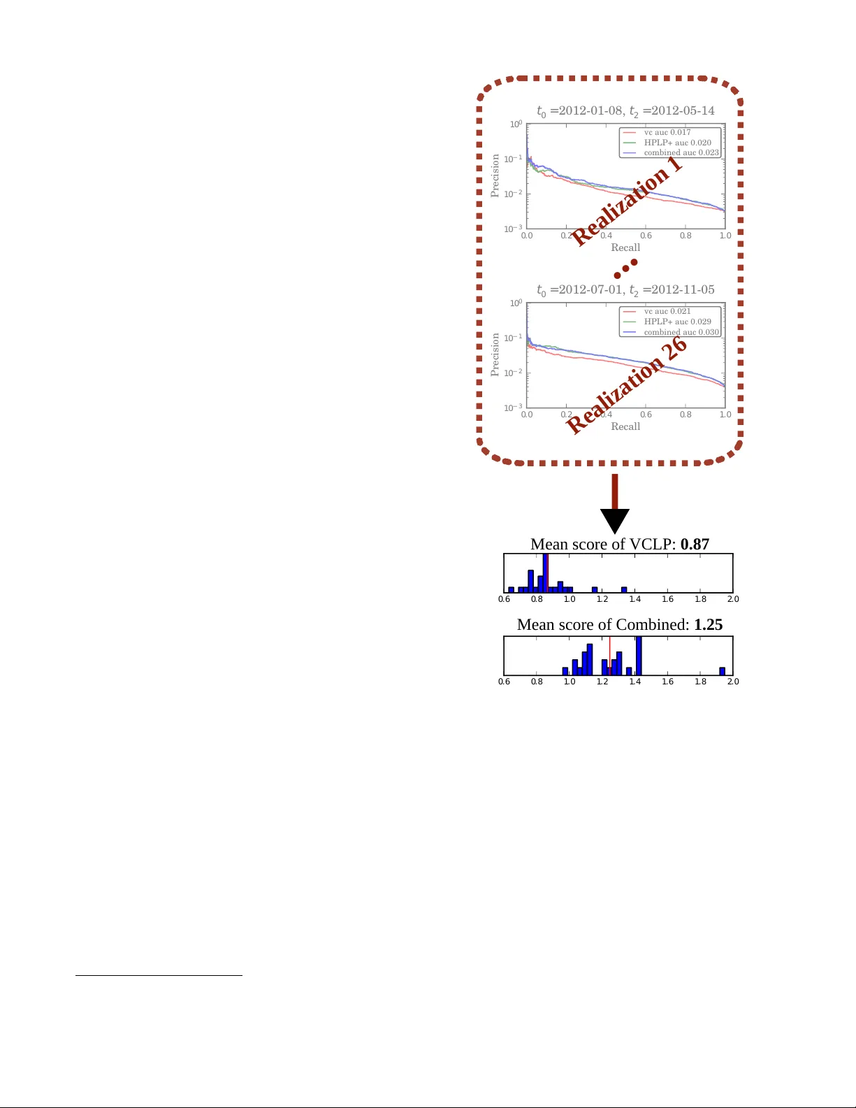
Link Prediction with Social V ector Cloc ks Conrad Lee University College Dublin conradlee@gmail.com Bobo Nick University of Konstanz bobo.nick@uni-konstanz.de Ulrik Brandes University of Konstanz ulrik.brandes@uni-konstanz.de Pádraig Cunningham University College Dublin padraig.cunningham@ucd.ie ABSTRA CT State-of-the-art link prediction utilizes combinations of complex features deriv ed from network panel data. W e here show that com- putationally less expensi ve features can achieve the same perfor- mance in the common scenario in which the data is av ailable as a sequence of interactions. Our features are based on social vec- tor clocks, an adaptation of the vector-clock concept introduced in distributed computing to social interaction networks. In fact, our experiments suggest that by taking into account the order and spac- ing of interactions, social vector clocks exploit different aspects of link formation so that their combination with previous approaches yields the most accurate predictor to date. Categories and Subject Descriptors H.2.8 [ Database Management: Database Applications — Data Mining ]: K eywords social networks, vector clocks, link prediction, online algorithms 1. INTR ODUCTION Link prediction deals with predicting previously unobserved in- teractions among actors in a network [1]. Predictions are based on the dynamic network of previously observ ed interactions, which is usually made av ailable in one of two forms: panel data or ev ent data. The former refers to a sequence of complete network snap- shots and typically contains only coarse-grained temporal informa- tion. Event data, on the other hand, consists of a finer-grained se- quence of single, time-stamped relational events, in which the ex- act minute or second of each e vent is known. Whereas panel data is often collected by means of longitudinal surve ys, ev ent data is typ- ically the outcome of automated data collection, such as log files of e-mail, phone, or T witter communication. It is possible to con vert network event data into (interv al-censored) network panel data; indeed, Liben-No well and Kleinber g [2] did so in their seminal paper which introduced the link prediction problem for social networks, and the practice has become standard [1, 3]. The con version is usually carried out by defining a sequence of time slices and aggregating relational ev ents within these time win- dows into static (weighted) networks. At the expense of losing the ordering and spacing of original ev ents, this con version allo ws one to employ the large set of tools that have been developed for static and longitudinal network analysis [4, 5]. Whether the con version from event to panel data is justifiable or not depends crucially on mechanisms which drive tie formation in a given network. For example, Liben-Nowell and Kleinberg [2] conducted experiments on future interactions in large co-authorship networks. In this setting, the exact sequence and spacing of publi- cation dates can hardly be relev ant because publications dates are distorted anyway (backlogs, preprints, etc.); aggregation of publi- cation events on a coarser time-scale thus does not appear to be problematic. In other situations the fine-grained temporal information may be highly relevant, making the con version from ev ent data to panel data dif ficult to justify because it may destroy important patterns of interaction; see [6] for a recent re vie w on general temporal network approaches to exploit such information. W ith regard to the link prediction problem, if we are trying to foresee whether node A will send an email message to B in the near future, for example, then an extremely useful piece of information is whether B has recently sent A a message; if so, it is likely that A will respond to B soon. This response-mechanism is known as r ecipr ocity , and has been observed to be highly rele v ant for predicting future ev ents in social networks [7]. By aggregating communication events into cross- sectional graphs, traditional link prediction schemes are generally prone to miss such simple and useful mechanisms. Here, we demonstrate that link predictors can indeed be made more effecti ve and efficient if they operate directly on appropriate time-stamped dyadic communication data, and as a result can take advantage of the information contained in the spacing and ordering of relational ev ents. The approach we introduce is based on keeping track of ho w out of date a node A is with respect to another node B with respect to time-respecting information flow , and for doing so we employ the concept of vector clocks. Our results confirm that dyadic features that exploit fine-grained temporal information can be highly relevant for predicting which actors will communicate for the first time in the near future, and are not limited to reciprocity . The outline is as follows: first, we describe the types of data for which we expect fine-grained temporal data to be relev ant for link prediction. Next, we revie w the link prediction problem for this type of data, paying particular attention to supervised link pre- diction, a frame work that we employ here. W e then specify how a modified version of social vector clocks can be used as a supervised link predictor, and proceed to evaluate this predictor . W e conclude with a discussion of our results, as well as possible future work. 2. MO TIV A TION In the introduction, we stressed that the ordering and spacing of communication events might contain valuable additional informa- tion ov er and above the mere number of contacts between a pair of actors. Consider the example in Figure 1, which depicts a series of directed communication ev ents, such as e-mail messages. Let us imagine that the actor represented by node A is in charge of or- ganizing a wellness weekend-trip for a group of friends, and that she keeps changing her mind about when and where to go. She Figure 1: Illustrativ e example of social network data containing fine-grained information on dyadic communication ev ents. Indirect information might flow on time-respecting paths, i.e. along labels that respect the ordering of time. Adapted from [16]. finally settles on a plan on Thursday at noon, and all of the sub- sequent messages she sends out include the final trip details. W e can ask: which nodes can possibly know them, giv en the observed interactions? Clearly , node A communicated with node C after she made up her mind on Thursday , so node C w ould ha ve recei ved the final information on Friday at 9am. Because node C subsequently sent node B a message, node B could also ha ve receiv ed the cor- rect information. On the other hand, nodes D and E could not have receiv ed information from node A that is more recent than W ednes- day at 3pm. T wo ke y and related concepts present in this e xample are latency and indirect updates . W e expect that groups of people who co- ordinate some action, such as a wellness weekend-trip, will need to synchronize their knowledge of certain key information such as departure time and destination. So in some sense (which we will define formally in Section 4) the members of this group hav e a lo w latency with respect to each other . Indirect updates, such as the one that made B aware of A ’ s latest trip plans, are an important mech- anism for maintaining these low latencies: ev en though B did not hav e an y direct message from A after she made up her mind, B still got the latest plans indirectly via C. This type of indirect communication is common in social sys- tems: consider the case of sev eral adult siblings who communicate with each other rarely , and more often communicate with their par- ents. In this case, the siblings’ information on each other can re- main up to date due to the central role of the parents, who provide the siblings with an indirect means of communication. More gen- erally , we observe that gossip – the information exchanged when two people talk about an absent third party – is a form of commu- nication prev alent in society and is in essence a form of indirect update. The moti vation behind our approach in this paper is that this dif- fusion of information via indirect updates is common in many so- cial systems, and can be exploited to infer future direct relations. In terms of the example above, we might predict that the siblings are likely to communicate with each other because their latencies with respect to each other remain low . Howe ver , the current approach to link prediction throws away much of these temporal clues by first con verting the e vent stream into panel data. In the datasets we analyze here, we also have reason to believ e that fine-grained diffusion patterns are relevant to link prediction. For instance, two of the datasets that we will use during our ev al- uation contain sequences of micro-blogging e vents that come from T witter . Bakshy et al. [8], e.g., hav e found that word-of-mouth in- formation in T witter spreads via many small cascades of tweets, mostly triggered by ordinary individuals. These small chains of diffusion are e xemplary of the indirect updates we described abov e, and by considering the details of how information spread, we may be able to infer which nodes will come into direct contact in the future. Detailed information on the datasets we use in our final ev aluation is given in Section 5.1. 3. LINK PREDICTION In this section, we re view the basics of link prediction. In partic- ular , we provide an ov erview of how machine learning models can be used to combine multiple link predictors – a technique called supervised link prediction. 3.1 The Problem and its Evaluation Along the lines of its original formulation by Liben-Nowell and Kleinberg [2], we formulate the link prediction problem for dyadic ev ent data as follows: Giv en a sequence of communication events in the form of (time, sender , recei ver) tuples, predict which pairs of nodes who had no communication (i.e. are discon- nected) in the time interval [ t 0 , t 1 ) will communicate (i.e. become connected) in the time interval [ t 1 , t 2 ) . 1 An unsupervised link pr edictor is a function which, gi ven a dyad (a pair of nodes) and the list of all previously occurring e vents, returns a score, where a higher score indicates that an edge is more likely to form in the dyad. Common neighbors is an example of an unsu- pervised link predictor: giv en a dyad (A,B), return the number of contacts shared by A and B. Although common neighbors is sim- ple, it is quite effecti ve and many of the most ef fectiv e unsupervised link predictors (such as the similarity measure originally proposed by Adamic and Adar [9]) are also based on shared neighbors [2, 3]. By running a link predictor on all dyads that are disconnected in the interval [ t 0 , t 1 ) , one can rank all of the possible new links. T o ev aluate a link predictor, we compare this ranking with the set of new dyads that actually occur in the period [ t 1 , t 2 ) . In practice, performance on the link-prediction task is often measured using R OC curves or measures based on precision, but in their recent pa- per on ev aluation in the link prediction problem, Lichtenwalter and Chawla [1] con vincingly ar gue that due to the e xtreme class imbal- ance present in the link prediction task, precision-recall curves are a more rele vant and less deceptive way to measure performance. For that reason, here we e xclusiv ely use precision-recall curves for our ev aluation. 3.2 Supervised link prediction As link prediction is fundamentally a binary classification prob- lem, it is natural to use the powerful binary classification models that ha ve been de veloped in machine learning. The primary advan- tage of this approach is the ability to combine multiple unsuper- vised link predictors into one joint prediction model. W e will now provide a brief overvie w of how supervised link prediction works. For an in-depth discussion of supervised link prediction, see [10]. As is usual in machine learning evaluation, we train and test our classifier on two separate datasets: we must be careful that the classifier is not trained on the same data that is used to ev aluate it. For this reason, supervised link prediction requires a train and test framework as depicted in the bottom half of Figure 2. A link prediction classifier is given a set of features related to each discon- nected dyad in the period [ t 0 , t 1 ) , as well as a label which indicates whether the dyad became connected in the period [ t 1 , t 2 ) . From 1 In practice, the specification of a link prediction task in volv es more details, such as whether directed or undirected dyads are con- sidered; we address these points in Section 5.2. this information, it learns a model which relates the dyad features to the probability that a previously disconnected dyad becomes con- nected. T o measure the accuracy of a link predictor , we then create a set of test dyad features in the interv al [ t 0 0 , t 0 1 ) and use those to score the test labels in the interval [ t 0 1 , t 0 2 ) . W e measure how accu- rately the scored dyads predict the set of test labels using the area under the precision-recall curve (A UPR). W e note that the A UPR of a link predictor can fluctuate greatly: as the behavior of users changes, so does the accuracy of the link predictor . In order to better estimate the typical A UPR attained by a link predictor, we can run this procedure many times; we will refer to each run of the procedure outlined in the bottom panel of Figure 2 as a realization . As shown in the top panel of Figure 2, we shift realizations such that the A UPR of each realization is mea- sured using a distinct set of ev ents. T ime T rain Classifier T est Classifier { { { { Events for creating dyad features Events for creating dyad labels t 0 t 2 t 1 t' 0 t' 2 t' 1 Dataset Begin Dataset End Realizati on 1 Realizati on 2 Realizati on 3 Realizati on 4 Realizati on k ... Figure 2: Framework for performing and ev aluating supervised link prediction. Each dataset is split into sev eral r ealizations ; each real- ization, in turn, is split into intervals to train and test a classifier . Lichtenwalter et al. [10] con vincingly argue that the link predic- tion problem should be stratified over different geodesic distances (i.e., path lengths). That is, the disconnected dyads with a geodesic distance of N = 2 , 3 , 4 , . . . should each be put into different bins, and a separate classifier should be trained on each bin. This strat- ification leads to better performance because the decision bound- ary for each bin can be quite different, with local features (such as common neighbors) being of primary importance at small dis- tances, and global features (such as preferential attachment) be- coming more important at larger distances. Thus, by treating each distance as a separate classification task, not only does performance improv e, but one can also gain insight into the particular strengths and weaknesses of a predictor . W e therefore follow suit and treat each distance as a separate link prediction task. 4. LEARNING WITH VECTOR CLOCKS Having introduced the necessary background on network ev ent data and link prediction, we now explain how fine-grained temporal information can be exploited, using the concept of v ector clocks. 4.1 T raditional V ector Clocks Figure 3: The basic idea of vector clocks: each node’ s vector clock (in grey) keeps track of the most recent information it could have on the other actors in the network. V ector clocks were conceptually defined in [11] and [12] as a means to track causality in concurrent systems, but had implic- itly been used before, e.g., in [13], with underlying foundations attributed to [14]; for an introduction to vector clock systems in distributed computing refer to [15]. Kossinets et al. [16] brought the concept to social network analysis by substituting message- exchanging processes with communicating indi viduals. In this spe- cial setting, the basic motiv ation of vector clocks is to keep track of the lower bound of how out-of-date a person is with respect to ev ery other person at any time, assuming that information spreads according to a giv en time-ordered list of communication ev ents. Reconsider the trip-planning example we introduced in Section 2. There we asked: which nodes could possibly know about the most recent details, through either direct or indirect updates? V ector clocks provide a way of answering this question by keeping track of the last possible update that a node could have receiv ed from each other node: the vector clock (grey box) next to node E in Figure 3 indicates that E cannot possibly have receiv ed information from A more recent than W ednesday at 3pm, that it could ha ve receiv ed no information whatsoe ver from nodes B and C, and so on. Each node is always assumed to ha ve up-to date information on itself. Formally , let ( t i , s i , r i ) , i ∈ N , a sequence of (time,sender ,re- ceiver) tuples satisfying t i ≤ t i +1 and s i 6 = r i . The set of individ- uals is defined implicitly by V = S i ∈ N { s i , r i } . At time t i , sender s i and receiver r i exchange direct information about themselves, and indirect information about others that result from communica- tion e vents in the past ( t < t i ). That is, information can not be forwarded instantaneously but with arbitrary small delay . Now , a vector clock is a multiv ariate function φ v,t = ( φ v,t ( u ) : u ∈ V ) , in which v ’ s temporal view φ v,t ( u ) on u at time t is defined as the time-stamp t ∗ ≤ t of the latest information from u that could have possibly reached v (directly or indirectly) until time t . At any time, each actor is up-to-date with respect to itself, φ v,t ( v ) = t . T empo- ral views on others can be tracked online as step functions resulting from component-wise maximum calculations of φ s i ,t i and φ r i ,t i at time-steps t i . Intuitively , φ s i ,t i is updated if and only if a commu- nication event is mutual (such as telephone con versations or meet- ings), while the update is restricted to φ r i ,t i if a communication ev ent is directed (such as email-, text-, or T witter-messages). A major dra wback of traditional vector clocks is poor scalability . This results from quadratic space requirements to maintain com- plete temporal views, along with efficiency problems when per- forming linear-size maximum calculations on ev ery event. There- fore, traditional vector clocks are too expensiv e to maintain and manipulate in large graphs. While quadratic space and linear band- width requirements are necessary to allow for exact calculations in the general case [17], approximate calculations of a limited number of temporal views [18] and less expansiv e update algorithms in re- stricted settings, such as acyclic communication graphs [19], have been proposed. For suitable topologies, additional data structures can be used to reduce the bandwidth of information to be forwarded [20]. 4.2 Social V ector Clocks In contrast to those enhancements stemming from the literature on distributed computing, we propose a modification that is tailored to social communication networks. While the original formulation of vector clocks is interesting for social networks because it cap- tures the process of gossip and indirect communication, it does so in an e xaggerated and almost clumsy manner . Experiments [21] on the small-world property of social networks [22, 23] and the in ves- tigation in [16] suggest that, in the vector clock update algorithm described abov e, nodes will soon receiv e huge amounts of infor- mation on people they hav e nev er met, and whom even their own contacts have never interacted with directly . Indeed, in our own initial experimentation, we found that most actors quickly attain a non-null temporal view with most other actors in the system, and that single communication e vents often cause an actor to be updated on nearly all of the other actors. These global updates are hard to justify because they do not seem to resemble social communication. In other words, while exchanging system-wide information is important in the context of distributed computing, such massiv e information exchanges do not occur when two people communicate with each other . Rather than updating each other on most of the other actors in the system, the nature of social communication is bounded by cognitiv e limits; such as the number of acquaintances, which does not scale with the size of the ov erall population [24]. W e observe that when two people meet and talk about third par- ties, they are likely to discuss mutual acquaintances, or at least re- strict the conv ersation to people at least one of them has met di- rectly . Compared to this circle of acquaintances and mutual ac- quaintances, they are relatively unlikely to talk about any given friend of a friend of a friend, whom neither knows directly . Based on this observation, we propose to bound the reach of indirect up- dates. Not only does this make the vector clock update process more closely approximate how indirect updates actually take place in social communication, but in practice this restriction also sub- stantially reduces the memory used by the algorithm, making it scale to large sparse social networks with millions of actors and billions of communication ev ents. Our modification adds one parameter µ to the vector clock frame- work, which restricts ho w far information can travel along time- respecting paths; we will also refer to this parameter as the r each of indirect updates. More precisely , the reach of indirect informa- tion is bounded by the minimal number of hops it e ver took a chunk of information to tra vel between a pair of actors on time-respecting paths. Consider the consequence of assigning the following v alues to µ : µ = 1 restricts the creation of temporal vie ws to those pairs of ac- tors that have already communicated directly: A node r can receiv e an indirect update on a node u if and only if this r e- ceiver r has previously had a direct update from u . µ = 2 additionally allo ws the creation of temporal views for dis- tance-two neighbors (where distance is measured using time- respecting paths). That is, when considering whether node r can recei ve an indirect update on a node u via a direct update from node s , it is always suf ficient that the sender s previ- ously had a direct contact with u . W e note that this case has been shown to be especially important in information broker- age [25]. µ = ∞ corresponds to the classical vector clock algorithm with unlimited information spread, and in practice quickly results in quadratic space requirements. This modification is straightforward to implement, because using the vector -clock framework, it is tri vial to track the length of short- est time-respecting paths: When processing a communication event ( t, s, r ) , the minimum number of hops it ev er took a chunk of in- formation about u to reach r is given by dist t i ( u, r ) = min( dist t i − 1 ( u, s ) + 1 , dist t i − 1 ( u, r )) , where dist t ( a, b ) refers to the length of the shortest time-respecting ( a, b ) -path until time t . In this way , distances are directed, respect- ing the ordering of ev ents, and decreasing over the course of time. In our implementation, distances are not known to the source of an information chain, but saved together with the vector clock of the target. Once a short information chain has been observed, a corresponding temporal view is established and also allowed to be updated by longer information chains. In practice, this modification reduces memory requirements very substantially . 4.3 A Link Predictor with Social V ector Clocks W e have described how social vector clocks can, in real time, keep track of the most recent information that could have possibly trav eled between pairs of nodes. While we compute the social vec- tor clocks, we can easily deriv e several features that may be useful for link prediction. These features can then be combined using a supervised link predictor as we outlined in Section 3.2. A first feature is immediately deri ved from the temporal views that are sa ved in the vector clocks: the curr ent latency is defined as the difference between the current time and the timestamp sa ved in the temporal vie w . As second and third features, we track the number of dir ect updates and indir ect updates that occur between a pair of actors as the vector clocks are computed. A fourth feature we calculate is the expected latency between each pair of nodes, which can be thought of as the best guess on how out-of-date an actor is about another at any point in the observation window . See Figure 4 for an illustration of all these features. Some users of a service like T witter may be much more acti ve than others. This heterogeneity will mean that some users will ha ve a latency of weeks with their closest contacts, whereas others will typically have a latency of days or hours with their closest contacts. Such heterogeneity may make it hard for a classifier to detect a observation time latency t 1 t 2 t 3 l 3 Figure 4: Deriving link prediction features from social vector clocks: Example of a dyad with two direct updates (at time t 1 and t 2 ; the new latency becomes zero), followed by one indirect up- date (at time t 3 ; the new latency is l 3 > 0 ). The current latency (solid line) is a linear jump function resulting from t − φ v,t ( u ) . The expected latency (dashed line) is the weighted mean of average la- tencies (dotted horizontal lines) between vector clock updates. N = 2 N = 3 N = 4 Dataset Realizations A vg. Pos. A vg. Neg. A vg. Pos. A vg. Neg. A vg. Pos. A vg. Neg. election 26 796 243658 186 922854 41 1373586 election2 26 1664 516415 583 1973244 198 2888931 olympics 12 182 15704 38 40257 10 42641 irvine 4 478 167674 675 536188 95 348814 studivz 23 1332 751172 706 5765692 - - T able 1: Link prediction statistics by dataset and path length N . These values report the av erage o ver all realizations of each e xperiment. For each realization, measurements are based on the graph associated with the interval [ t 0 0 , t 0 1 ) and the new edges formed in the interv al [ t 0 1 , t 0 2 ) . decision boundary; for this reason, in addition to keeping track of the absolute values of the current and expected latencies, we keep track of the ranks. That is, from the perspectiv e of a given node i , we sort each of i ’ s temporal views by their current latency , and then rank the corresponding dyads—this yields an additional feature for each dyad { i, j } . W e do the same for the expected latency . So far we have described six features for each dyad: the current latency (both absolute v alue and rank), the expected latency (abso- lute value and rank), the number of direct updates, and the number of indirect updates. All of these features can be kept track of in real time and in practice they add little computational ov erhead. In the context of directed link prediction, for each directed dyad we can keep track of all six of these features in both directions, yield- ing twelve features. Finally , our definition of social vector clocks included one parameter µ which bounds how far information can trav el. In practice one might not kno w which value of this parame- ter will lead to the best results; in such a case, one can simply run multiple instances of the vector clocks in parallel, each with a dif- ferent value of the reach parameter , and combine all the resulting features. A classifier can then learn which feature set is the most informativ e. For example, in our evaluation below , we run reach- parameterized vector clocks with three different reach parameters: 1, 2, and ∞ , which creates a total of 36 features for each directed dyad. 5. EV ALU A TION & RESUL TS 5.1 Datasets T wo of the datasets we consider come from T witter . While T wit- ter is often used as a medium for impersonally broadcasting mes- sages to large numbers of followers, it also supports more targeted forms of communication, in which users explicitly refer to each other . This targeted (although public) communication occurs in the form of retweets (in which one user rebroadcasts another users tweet, and attributes the tweet to its source) and user mentions, where the @ symbol is used to explicitly refer to a user . In the T witter data that we analyze here, we filter T witter datasets to in- clude only this targeted form of communication (i.e., those with retweets or user mentions). W e remov e self loops, and if a tweet mentions more than one user , we turn it into as many ev ents as there are users mentioned in the tweet. With this representation, the data corresponds to the basic scenario of dyadic communica- tion event streams underlying our in vestigation: we are given a sequence ( t i , s i , r i ) , i ∈ N , of (time,sender,recei ver) tuples sat- isfying t i ≤ t i +1 and s i 6 = r i . T witter UK Olympics Data The olympics dataset covers T wit- ter communication among a set of 499 UK Olympic athletes ov er the course of the 18 months leading up to the 2012 Sum- mer Olympic Games, including 730,880 tweets. It was intro- duced in [26] and is based on a list of UK athletes curated by The T ele graph . 2 W e remove all tweets that are not user men- tions or retweets between this core set of 499 users, a step which reduces the dataset to 93,613 tweets among 486 users. T witter US Elections Data Similar to the olympics dataset, the election dataset is based on a curated list of T witter users, in this case curated by Storyful, a commercial news gather- ing platform targeted at journalists. One of Storyful’ s fea- tures is topical T witter lists, which journalists can subscribe to in order to remain well informed on a gi ven topic. Here we scraped tweets by users on Storyful’ s US 2012 Presiden- tial election list. In addition we added the T witter accounts of all those candidates seeking of fice at the lev el of go vernor , US Senator , or member of the US House of Representativ es. In total, this dataset covers the date range from Jan. 1st 2012 to Nov . 9th, 2012, and includes 392,662 user mentions and retweets among 2447 T witter accounts. Additionally , we cre- ated an extended version of this dataset, which we will refer to as election2 , by collecting the tweets associated with T witter users who were often mentioned in election . This extended dataset includes 546,329 tweets among 5,632 users ov er the same date range as election . StudiVZ W all posts StudiVZ was created in 2005 as a German competitor for international online social networks. F or sev- eral years it was the most popular online social network in Germany , although it has recently been overtaken by Face- book. The studivz dataset we examine here is based on a crawl of a single univ ersity’ s subnetwork; it is described in [27]. While in [27] the static friendship network is an- alyzed, here we focus on the wall post (“Pinnwand”) data. The dataset is the largest we look at here, containing 26,180 nodes and 886,241 ev ents. UC Irvine Panzarasa et al. [28] introduced an event-based dataset which comes from a social netw orking site set up for the stu- dents of the Uni versity of California at Irvine. Each event in this dataset is a message—it is unclear whether these are priv ate or public messages. While the dataset covers a period from April to October 2004, the great majority of the events occur between mid April and mid June. Starting in mid June, there is a two week period in which no events occur , and for the remainder of the dataset very few messages are sent. For this reason, we look only at the period from April 10th to June 15th. 5.2 Experiment Setup The “high-performance” link predictor (HPLP+) introduced in [10] is a state of the art link predictor which combines some of the 2 twitter.com/#!/Telegraph2012/london2012 strongest unsupervised link predictors. In the following experi- ments, HPLP+ acts as the baseline predictor and our objecti ve is to ev aluate the performance of the vector clock link predictor (VCLP) described in Section 4.3, and a combined predictor which uses the features from both VCLP and HPLP+. 3 Framing a supervised link prediction task requires se veral pa- rameters. One important parameter is the choice of classifier: as in [10], we used bagged forests, a technique suited for the ex- tremely imbalanced classes found in link prediction. Howe ver , rather than bagging ten random forests, we bag ten Stochastic Gra- dient Boosting classifiers. W e use the implementation provided in the scikit-learn python package [30], using 1000 trees in each clas- sifier , setting the learning rate to 0.005, and subsampling rate to 0.5. In each bag we sampled from the positiv e instances with replace- ment, and undersampled from the negati ve instances with replace- ment such that the class imbalance ratio was 10 negati ve for ev ery positiv e. Another important experimental parameter is whether the link prediction is directed or undirected. In all of our datasets, edge di- rection is highly relev ant—for example, I might mention President Obama in a tweet, but Obama mentioning me in a tweet would have a completely different meaning. For this reason, we restrict our ev aluation to directed link prediction. As one can see in T able 1, as the directed geodesic distance ( N ) in the link prediction task increases, classes become sev erely imbalanced, and in the case of olympics , hardly an y new links form. In olympics in general, the classifier has very little positiv ely labeled data to train on, which increases the risk of ov erfitting when extra features are added. W e must also specify some parameters related to the width of the temporal windows used in the evaluation. In principle, we wanted to make the duration of training period long enough so that a clear and stable snapshot of the network has emerged, and then ev alu- ate on ev ents that occur just after the end of the training period. Therefore, wherever possible we used a training window of 120 days and a test window of 7 days. (In other words, the width of the red bars in Figure 2 is 120 days and the width of the blue bars is 7 days.) Howe ver , given the short duration of the UC Irvine dataset, we use a shorter training period than in the other datasets, and are not able to run as many realizations of our ev aluation; we set the training period to 28 days. Furthermore, the small size of olympics meant that in the seven day test period very few new links emerged, leaving the classifier with too little data to train on. Thus, for olympics we set the test width to 14 days. 5.3 Experiment Evaluation The number of realizations performed on each dataset is indi- cated in T able 1. For each realization, we record the precision- recall curve of each predictor , leaving us with a sequence of pre- cision-recall plots such as those presented in the upper section of Figure 5. W e are interested in ho w VCLP and the combined predic- tor perform relative to HPLP+, so we summarize them as follows (as outlined in Figure 5): W e treat the performance of HPLP+ as the baseline, and in each plot, we measure the area under HPLP+’ s precision-recall curve. W e then record the area under the precision- recall curve (A UPR) of both VCLP and the combined predictor as a fraction of HPLP+’ s A UPR. Thus, if in one realization HPLP+’ s A UPR is 0 . 020 and the combined predictor’ s A UPR is 0 . 024 , then we record the combined predictor’ s score as 1 . 2 . After recording this score for all realizations, we are left with a distributions of scores as in the histogram in Figure 5. By taking the av erage of these scores, we can characterize in a single number how much 3 W e use the LPMade link prediction framework to compute HPLP+; this is the author’ s reference implementation [29]. 0 . 0 0 . 2 0 . 4 0 . 6 0 . 8 1 . 0 Reca ll 1 0 − 3 1 0 − 2 1 0 − 1 1 0 0 Prec isi on t 0 = 201 2-0 7-0 1, t 2 = 201 2-1 1-0 5 vc auc 0.0 21 HPL P+ auc 0.0 29 comb ined auc 0.03 0 0 . 0 0 . 2 0 . 4 0 . 6 0 . 8 1 . 0 Reca ll 1 0 − 3 1 0 − 2 1 0 − 1 1 0 0 Prec isi on t 0 = 201 2-0 1-0 8, t 2 = 201 2-0 5-1 4 vc auc 0.0 17 HPL P+ auc 0.0 20 comb ined auc 0.02 3 Realization 26 ... Mean score of VCLP : 0.87 Mean score of Combined: 1.25 0 . 6 0 . 8 1 . 0 1 . 2 1 . 4 1 . 6 1 . 8 2 . 0 0 . 6 0 . 8 1 . 0 1 . 2 1 . 4 1 . 6 1 . 8 2 . 0 Realization 1 Figure 5: An overvie w of how we scored the link prediction task. Link predictors are first run on each realization of the experiment. In each realization, precision-recall curves are constructed. The A UPR for each predictor is then measured, and the A UPR of VCLP and the combined link predictor is then divided by the A UPR of HPLP+; this score is the relative performance of each predictor with HPLP+ as the baseline. For each dataset, the av erage of these scores is then reported; stratified ov er different geodesic distances. better or worse VCLP and the combined predictor perform than HPLP+. W e report these av erages for each experiment in T able 2a; see next section for discussion. 5.4 Results In T able 2a, we see that VCLP on its own performs comparably to HPLP+. Considering that HPLP+ combines a broad range of so- phisticated graph features, we were surprised to see VCLP perform similarly . Moreover , all network statistics employed by the pro- posed VCLP can be kept track of online, directly on the list of com- munication ev ents, while many of the statistics included in HPLP+ T able 2: A verage performance of supervised link predictors relativ e to HPLP+. election election2 olympics irvine studivz N 2 3 4 2 3 4 2 3 4 2 3 4 2 3 4 VCLP 0.87 0.86 1.05 0.92 0.75 0.86 0.97 1.07 1.06 1.11 1.87 1.12 1.17 1.20 - Combined 1.25 1.15 1.00 1.43 1.38 1.15 1.08 1.10 1.06 1.33 1.65 1.13 1.39 1.22 - (a) Results on predicting all edges at different distances ( N = 2 , 3 , 4 ); see 5.4 for discussion. election election2 olympics irvine studivz N 2 3 4 2 3 4 2 3 4 2 3 4 2 3 4 VCLP 0.75 0.78 0.99 0.82 0.65 0.79 0.75 1.02 1.23 0.95 0.79 1.00 0.49 0.57 - Combined 1.17 1.05 1.00 1.38 1.34 1.17 1.06 1.01 1.00 1.19 1.23 1.03 1.11 1.04 - (b) Results on predicting non-reciprocal edges at different distances; see section 5.5 for discussion. hav e to be recalculated whene ver new links are added to the net- work. Consequently , our results suggest that link prediction with vector -clock statistics can be performed much more efficiently in any situation, where the model parameters are learned beforehand and applied in real-time on a growing sequence of “test” e vents. When the features of VCLP and HPLP+ are combined, the per- formance increase ov er HPLP+ is substantial. In general, the per- formance gain is largest when we are predicting links on dyads that have a geodesic distance N = 2 . Performance gain decreases for greater N , suggesting that VCLP features are most useful for predicting local links rather than long-range links ( irvine is an exception to this trend, where N = 3 sees by far the largest boost to performance). The improv ement is smallest on olympics , per - haps because the classifier struggles with the small number of pos- itiv e training examples. Giv en that stand-alone VCLP and HPLP+ yield similar predic- tion accuracy , it is interesting to observe the added value of comb- ing both predictors. In other words, there appear to be qualitativ e differences in the network effects that can be captured in the VCLP and HPLP+ framew ork. 5.5 Controlling f or reciprocity Imagine we’ re trying to predict whether a node A will soon send its first mes sage to D. One of the features included in VCLP is D’ s current latency with A through direct updates – in other words, how many seconds hav e elapsed since D sent a message to A. Given the significance of reciprocity , this feature will be e xtremely useful for cases where D has just sent a message to A. It could be the case that this feature alone – which is trivial to keep track of without vector clocks – is responsible for all of the benefit that comes from VCLP. In that case, we could simply keep track of this single feature and forget about v ector clocks. T o measure whether this is the case, we run the entire e valuation again, but e xclude all dyads where D has had any direct contact with A; see Figure 6. The results presented in T able 2b are in the same units as the results presented in T able 2a. W e observe that the performance of VCLP does indeed drop, but that there is still a significant benefit provided by combining the features of VCLP and HPLP+. Again, we stress that the lackluster performance on olympics may be due to the small number of new links that form, which provides v ery few positi ve training e xamples. 6. SUMMAR Y The current approach used by state of the art link predictors is Figure 6: The directed dyad (A, D) has a geodesic distance of 3, b ut the distance of dyad (D, A) is 1. This dyad would be included in the experiments whose results are presented in T able 2a, b ut would be e xcluded from the experiments whose results are presented in T able 2b. to operate in a panel data setting, in which finer-grained temporal information is ignored. In cases where link formation is not driven by cascades of information, such an approach might be appropriate. Regarding co-authorship networks, for instance, precise informa- tion on the sequence and spacing of events may be largely irrele vant or ev en misleading, and so it may be reasonable to aggregate a way information on exact publication dates. Howe ver , in some net- works – such as the T witter retweet/mention networks mentioned here – information cascades are an important mechanism for driv- ing the formation of edges. In such a setting, the information con- tained in the exact sequence and spacing of events is highly rele- vant, and so the approach commonly employed in link prediction – to simply aggre gate ev ent data into panel data – is highly question- able. For example, the mechanism of reciprocity has been shown to be important in the context of directed link prediction. Thus, if we are trying to predict whether A will send a message to B, then an extremely useful piece of information is whether B has recently sent A a message; if so, it is likely that A will respond to B. By aggregating all e vents into a static graph, traditional link prediction schemes cannot exploit such simple and useful mechanisms. Our results suggest that dyadic features that exploit fine-grained temporal information beyond reciprocity are highly relev ant for predicting which actors will communicate for the first time in the near future. The approach we introduce here, called the V ector Clock Link Predictor (VCLP), is based on keeping track of the la- tencies between all presumably relev ant pairs of actors. The basic idea is to exploit information on how out of date a node A is with respect to another node B, and for doing so we adopt the concept of vector clocks. As an essential modification, we parameterized the traditional vector-clock concept to bound the reach of indirect information. Not only does this make the vector-clock update pro- cess more closely approximate how indirect updates actually take place in social communication, but in practice this restriction also dramatically reduces the memory used by the algorithm, thus mak- ing it applicable to large sparse social networks with millions of actors and billions of communication ev ents. W e have demonstrated that binary classifiers can indeed exploit actor latencies to improve accuracy in link prediction. Even HPLP+, a classifier which utilizes a wide range of graph features based on aggregated panel data, can perform substantially better when provided with additional features based on vector clocks. More- ov er , VCLP on its o wn already performs comparably to HPLP+, which allows for much more ef ficient link prediction in any situ- ation where the model parameters are learned beforehand and ap- plied in real-time on a growing sequence of e vents. Both of the supervised link prediction schemes considered here are based on many features, and by adding or removing various features many variations of social vector clocks are conceivable. Even with the intuitive motiv ation for social v ector clocks and their demonstrated performance, we hav e not necessarily advanced the understanding of the actual mechanisms behind link formation. W e are keen to gain more detailed insight into the link prediction prob- lem for specific types of interaction, e.g., by combining feature- selection schemes and more elaborate substantiv e theories. References [1] R. Lichtenwalter and N. V . Chawla. Link prediction: fair and effecti ve ev aluation. In Pr oc of ASONAM , pages 376–383, 2012. [2] D. Liben-Nowell and J. Kleinberg. The link prediction prob- lem for social networks. In Proc of A CM CIKM , pages 556– 559, 2003. [3] L. Lü and T . Zhou. Link prediction in complex networks: A surve y. Physica A: Statistical Mechanics and its Applications , 390(6):1150–1170, 2011. [4] S. W asserman and K. Faust. Social Network Analysis: Meth- ods and Applications . Cambridge Univ ersity Press, 1994. [5] T . A. B. Snijders. Models for Longitudinal Network Data. In P . Carrington, J. Scott, and S. W asserman, editors, Mod- els and methods in social network analysis , pages 215–247. Cambridge Univ ersity Press, 2005. [6] P . Holme and J. Saramäki. T emporal networks. Physics Re- ports , 519(3):97–125, 2012. [7] U. Brandes, J. Lerner , and T . A. Snijders. Networks Ev olving Step by Step: Statistical Analysis of Dyadic Ev ent Data. In Pr oc of ASONAM , pages 200–205, 2009. [8] E. Bakshy , J. M. Hofman, W . A. Mason, and D. J. W atts. Ev- eryone’ s an influencer: quantifying influence on twitter . In Pr oc of ACM WSDM , pages 65–74, 2011. [9] L. A. Adamic and E. Adar . Friends and neighbors on the web. Social Networks , 25(3):211–230, 2003. [10] R. Lichtenwalter , J. Lussier , and N. V . Chawla. New perspec- tiv es and methods in link prediction. In Proc of ACM CIKM , pages 243–252, 2010. [11] C. Fidge. Timestamps in message-passing systems that pre- serve the partial ordering. In Proc 11th Australian Computer Science Confer ence , pages 56–66, 1988. [12] F . Mattern. V irtual time and global states of distributed sys- tems. In Proc W orkshop on P arallel and Distrib uted Algo- rithms , pages 215–226, 1989. [13] D. S. Parker , G. J. Popek, G. Rudisin, A. Stoughton, B. J. W alker , E. W alton, J. M. Chow , D. Edwards, and S. Kiser . De- tection of mutual inconsistency in distributed systems. IEEE T rans. Softw . Eng. , 9(3):240–247, 1983. [14] L. Lamport. T ime, clocks, and the ordering of ev ents in a distributed system. Commun. ACM , 21(7):558–565, 1978. [15] R. Baldoni and M. Raynal. Fundamentals of distributed com- puting: A practical tour of vector clock systems. IEEE Dis- tributed Systems Online , 3(2), 2002. [16] G. K ossinets, J. Kleinberg, and D. W atts. The structure of information pathways in a social communication network. In Pr oc of ACM SIGKDD , pages 435–443, 2008. [17] B. Charron-Bost. Concerning the size of logical clocks in distributed systems. Inf. Pr ocess. Lett. , 39(1):11–16, 1991. [18] F . J. T orres-Rojas and M. Ahamad. Plausible clocks: constant size logical clocks for distributed systems. Distrib. Comput. , 12(4):179–195, 1999. [19] S. Meldal, S. Sankar , and J. V era. Exploiting locality in main- taining potential causality . In Pr oc of ACM PODC , pages 231–239, 1991. [20] M. Singhal and A. Kshemkalyani. An efficient implementa- tion of vector clocks. Inf. Pr ocess. Lett. , 43(1):47–52, 1992. [21] J. Kleinberg. The small-world phenomenon: an algorithm perspectiv e. In Pr oc 32nd annual ACM Symposium on Theory Of Computing , pages 163–170, 2000. [22] S. Milgram. The small world problem. Psychology T oday , 1 (1):61–67, 1967. [23] D. J. W atts and S. H. Strogatz. Collectiv e dynamics of small- world networks. Nature , 393(6684):440–442, 1998. [24] R. Hill and R. Dunbar . Social network size in humans. Human Natur e , 14:53–72, 2003. [25] R. S. Burt. Secondhand brokerage: Evidence on the impor - tance of local structure for managers, bankers, and analysts. Academy of Management , 50(1):119–148, 2007. [26] D. Greene, D. O’Callaghan, and P . Cunningham. Identifying topical twitter communities via user list aggregation. arXiv pr eprint arXiv:1207.0017 , 2012. [27] C. Lee, T . Scherngell, and M. J. Barber . In vestigating an on- line social network using spatial interaction models. Social Networks , 33(2):129–133, 2011. [28] P . Panzarasa, T . Opsahl, and K. Carley . Patterns and dynam- ics of users’ behavior and interaction: Network analysis of an online community . American Society for Inf Science and T echnolog , 60(5):911–932, 2009. [29] R. Lichtenwalter and N. V . Chawla. LPmade: Link Prediction Made Easy. The Journal of Machine Learning Researc h , 12: 2489–2492, 2011. [30] F . Pedregosa, G. V aroquaux, A. Gramfort, V . Michel, B. Thirion, O. Grisel, M. Blondel, P . Prettenhofer, R. W eiss, V . Dubourg, J. V anderplas, A. Passos, D. Cournapeau, M. Brucher , M. Perrot, and E. Duchesnay . Scikit-learn: Ma- chine Learning in Python. Journal of Machine Learning Re- sear ch , 12:2825–2830, 2011.