Boltzmann Machines and Denoising Autoencoders for Image Denoising

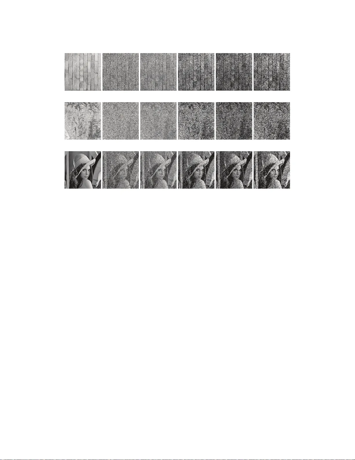
Boltzman n Machines and Denoising A utoencode rs f or Image Denoisin g K yungHyun Cho Aalto Univ ersity School of Science Departmen t of Information and Computer Science Espoo, Finland kyunghyun.ch o@aalto.fi Abstract Image denoising based on a p robab ilistic model of local image patches has been employed by v arious researchers, and recently a deep ( denoising ) autoencoder has been prop osed by Burger et al. [2012] and Xie et al. [2012] as a good model fo r this. In this paper , we propose that another popular family o f mo dels in th e field of deep learning , called Boltzman n machin es, can perf orm image d enoising a s well as, or in cer tain cases o f h igh level of noise, better than deno ising autoen coders. W e empirically ev aluate the two mo dels on three different sets of images with different types and lev els of no ise. Thr ougho ut the experiments we also examin e the effect o f the depth o f the mod els. The experiments confirmed our claim an d revealed that the perfor mance can be imp roved by ad ding mo re hidden layer s, especially when the le vel of noise is high. 1 Intr oduction Numerou s approa ches based on machine learn ing h av e been p ropo sed fo r image d enoising tasks over time. A do minant appro ach has been to p erform deno ising based on local statistics over a whole image. For instance, a method denoises each small image patch extracted from a whole noisy image and r econstructs the clean image from the denoised patches. Under this app roach, it is p ossible to use raw pixels of each im age patch [see, e.g. Hyv ¨ arinen et al., 1999] or the representatio ns in ano ther domain, for instance, in wa velet domain [see, e.g. Portilla et al., 2003]. In the case of using raw pixels, sparse coding has been a method o f choice. Hyv ¨ arinen et al. [1999] propo sed to use ind ependen t componen t analysis (ICA) to estimate a d ictionary of spar se elemen ts and compute the sparse code of image patches. Subsequen tly , a shrink age n onlinear function is applied to th e estimated sp arse co de elemen ts to suppr ess those elem ents with small abso lute mag- nitude. This spar se cod e elem ents are used to reconstruc t a noise- free image p atch. M ore recently , Elad and Aharon [200 6 ] also showed that sparse overcomplete representation is useful in denoising images. Some research ers c laimed that b etter d enoising perf ormanc e can be achieved b y using a variant of sparse coding methods [see, e.g. Shang and Huang, 2005, Lu et al., 2011]. In essence, these app roaches build a pr obabilistic mode l of n atural image patch es u sing a lay er of sparse laten t variables. The p osterior d istribution of each no isy patch is either exactly com puted or estimated, and th e noise-fr ee patch is re constructed as a n expectation of a condition al distribution over the posterior distribution. Based o n th is inter pretation, som e research ers h av e pr oposed very recently to utilize a ( probab ilis- tic) m odel that has more than one lay ers o f latent variables for image den oising. Bu rger et al. [2012 ] showed th at a deep multi-lay er p erceptro n that learns a mapping f rom a noisy image patch to its correspo nding clean version , can pe rform a s go od as the state-o f-the-art deno ising metho ds. Simi- larly , Xie et al. [ 2012] pr oposed a variant o f a stacked den oising au toencod er [V incent et al., 2 010] 1 that is mor e effecti ve in image d enoising. They were also able to show that the d enoising appr oach based on deep n eural networks perfor med as good as, or sometimes be tter th an, th e conventional state-of-the- art methods. Along t h is line of research, we aim to pr opose a yet ano ther type of deep neural net- works for image denoising , in this paper . A Gau ssian-Bernou lli restricted Boltzmann m a- chines (GRBM) [Hinto n and Salakhutdinov , 2 006] and deep Boltzma nn machines (GDBM) [Salakhutd inov and Hinton, 2009, Cho et al., 2011 b] are empir ically shown to pe rform well in im - age d enoising, compared to stacked den oising autoenco ders. Furth ermore, we extensively ev alu- ate the effect o f th e numb er of hidden layers of both Boltzmann m achine-b ased deep m odels a nd autoenco der-based one s. The emp irical e valuation is cond ucted using different noise types and lev- els on three different sets of images. 2 Deep Neural Networks W e start by briefly describing Boltzmann machin es an d denoising autoencoders which hav e become increasingly popu lar in the field of machine learning. 2.1 Boltzmann Machines Originally pro posed in 1 980s, a Boltzmann mac hine (BM) [Ackley et al., 1985] and especially its structural constrain ed version, a restricted Boltzm ann machine (RBM) [Sm olensky, 1986] have be- come inc reasingly im portant in mach ine learnin g since [Hinton and Salakhutdin ov , 2006] showed that a p owerful deep neur al network can b e tr ained ea sily b y stacking RBMs on top of each other . More re cently , an other variant of a BM, called a deep Boltzma nn mach ine (DBM), has been pr o- posed an d shown to outp erform o ther conventional m achine learnin g methods in many tasks [ see, e.g. Salakhutd inov and Hinton, 20 09]. W e first describ e a Gau ssian-Bernou lli DBM (GDBM) tha t has L lay ers of b inary h idden units an d a single layer of Gaussian visible units. A GDBM is defined by its energy function − E ( v , h | θ ) = X i − ( v i − b i ) 2 2 σ 2 + X i,j v i σ 2 h (1) j w i,j + X j h (1) j c (1) j + L X l =2   X j h ( l ) j c ( l ) j + X j,k h ( l ) j h ( l +1) k u ( l ) j,k   , (1) where v = [ v i ] i =1 ...N v and h ( l ) = h h ( l ) j i j =1 ...N l are N v Gaussian visible u nits and N l binary hidden units in the l -th hidd en layer . W = [ w i,j ] is the set of weigh ts b etween the visible neur ons and the first lay er hidden n eurons, while U ( l ) = h u ( l ) j,k i is the set of weights be tween the l -th and l + 1 -th hidden neu rons. σ 2 is the shar ed variance of the co nditional distribution o f v i giv en the hidden units. W ith the energy function, a GDBM can assign a pro bability to each state vector x = [ v ; h (1) ; · · · ; h ( L ) ] using a Boltzmann distrib ution : p ( x | θ ) = 1 Z ( θ ) exp {− E ( x | θ ) } . Based on this pro perty the parameters can be learned b y maximizing the log-likelihoo d L = P N n =1 log P h p ( v ( n ) , h | θ ) given N training samp les { v ( n ) } n =1 ,...,N , where h =  h (1) ; · · · ; h ( L )  . Although the upd ate rules b ased on the g radients of the log -likelihood functio n are well de- fined, it is intractable to exactly compu te them. Hence, an appro ach that u ses variational approx imation to gether with Markov chain Monte Carlo (MCMC) s am pling was proposed by Salakhutdin ov and Hinton [20 09]. 2 It has, however , b een f ound th at tr aining a GDBM u sing this app roach startin g fro m ran domly in itial- ized param eters is not trivial [Salakhu tdinov an d Hinton, 2 009, Desjardin s et al., 20 12, Cho et al., 2012]. Hence, Salak hutdinov and Hinton [20 09] and Cho et al. [20 12] pro posed pretra ining algo- rithms that can initialize the para meters of DBMs. In this paper, we u se the pr etraining alg orithm propo sed by Cho et al. [2012]. A Gaussian- Bernoulli RBM (GRBM) is a specia l case of a GDBM, where th e numb er of hidden layers i s restricted t o one, L = 1 . Due to this restriction it is p ossible to compute the posterior distri- bution over the hidd en units con ditioned on th e v isible un its exactly and trac tably . T he c ondition al probab ility of each hidden unit h j = h (1) j is p ( h j = 1 | v , θ ) = f X i w ij v i σ 2 + c j ! . (2) Hence, the positive par t of the g radient, that need s to be approxima ted with variational appr oach in th e case of GDBMs, can be computed exactly an d efficiently . Only the n egativ e part, which is computed over the mod el distribution, still relies on MCMC sampling, or more appr oximate method s such as contrastive divergence (CD) [Hinton, 200 2]. 2.2 Denoising A utoencoders A de noising au toencod er (DAE) is a special for m of multi-layer perceptr on n etwork with 2 L − 1 hidden layers and L − 1 sets o f tied weights. A DAE tries to learn a network that recon structs an input vector optimally by minimizing the follo wing cost function : N X n =1    W g (1) ◦ · · · ◦ g ( L − 1) ◦ f ( L − 1) ◦ · · · ◦ f (1)  η ( v ( n ) )  − v ( n )    2 , (3) where f ( l ) = φ ( W ( l ) ⊤ h ( l − 1) ) and g ( l ) = φ ( W ( l ) h (2 L − l ) ) are en coding and deco ding fu nctions fo r l -th layer with a compon ent-wise nonlin earity function φ . W ( l ) is the weig hts betwe en th e l -th an d l + 1 -th layers and is shared by th e enco der and deco der . For notational simplicity , we omit biases to all units. Unlike an ordin ary autoen coder, a DAE exp licitly sets som e of the com ponen ts o f an inpu t vector random ly to zero du ring lear ning via η ( · ) which explicitly adds no ise to an in put vector . It is usual to combine two d ifferent typ es o f no ise when using η ( · ) , w hich ar e additive isotropic Gaussian noise and ma sking no ise [V incent et al., 20 10]. The first typ e ad ds a zero-mea n Gaussian n oise to each input component, while the masking noise sets a set of randomly chosen input co mpon ents to zeros. Then, the D AE is trained to denoise the corrupted input. T rainin g a D AE is straightfo rward using backpropag ation algor ithm which computes the gradient of the objecti ve function using a chain-ru le and dyna mic p rogra mming. V incent et al. [2010] p ropo sed that training a d eep DAE beco mes easier when the weights of a deep D AE are initialized by gr eedily pretrainin g each layer of a deep D AE as if it were a single-layer D AE. In the follo wing experiments section, we follow this approach to initialize the weights and subsequently finetun e the network with the stochastic backpro pagation. 3 Image Denoising There are a numb er o f ways to perform image denoising. I n this paper, we are interested in an approa ch that relies on local statistics of an image. As it ha s been mentio ned ea rlier , a noisy large image can be den oised by deno ising small p atches of the imag e and com bining them togeth er . L et us defin e a set of N bina ry matr ices D n ∈ R p × d that extract a set o f small image p atches giv en a large, wh ole image x ∈ R d , whe re d = w hc is th e produ ct of the width w , the heig ht h and th e num ber o f colo r channe ls c of the image and p is the size 3 of image p atches (e.g., n = 64 if a n 8 × 8 imag e patch). The n, the denoised i ma ge is constructed by ˜ x = N X n =1 D ⊤ n r θ ( D n x ) ! ⊘ N X n =1 D ⊤ n D n 1 ! , (4) where ⊘ is a eleme nt-wise division and 1 is a vecto r of ones. r θ ( · ) is an im age den oising functio n, parameteriz ed by θ , that deno ises N imag e patches e xtr acted from the input image x . Eq. ( 4) essentially extracts a nd d enoises all possible image patches from the inp ut imag e. Then , it combines them by taking an av erag e of those ov erlap ping pix els. There ar e sev era l flexibilities in co nstructing a m atrix D . The m ost obvio us one is the size of an image patch . Althoug h there is no stan dar d approac h, many previous attempts tend to use patch sizes as s mall as 4 × 4 to 17 × 17 . An other one, called a stride, is the number of p ixels b etween tw o consecutive patches. T aking ev ery possible patch is one op tion, while one may opt to overlappin g patches by only a few pixels, which would reduce the comp utational complexity . One of the popular choice s for r θ ( · ) has b een to constru ct a probabilistic mode l with a set o f latent variables that d escribe natur al image patc hes. For instance, sparse co ding which is, in essence, a probabilistic mo del with a single layer of latent v ariab les has been a common choice. Hyv ¨ arinen et al. [199 9 ] u sed ICA and a n onlinear shrinkage function to comp ute the sparse code of an image patch, while Elad and Aharon [200 6 ] u sed K-SVD to b uild a spar se code dictionary . Under this a pproach denoising can b e conside red as a two-step recon struction. I nitially , th e posterio r distribution over the laten t variables is comp uted, or estimated, gi ven an imag e patch. Given the estimated p osterior distribution, the cond itional distribution, or its m ean, over the visible units is computed and used as a denoised image patch. In the following subsections, we descr ibe how r θ ( · ) can be implem ented in the cases of Boltzmann machines and denoising autoenc oders. 3.1 Boltzmann machines W e consid er a BM with a set of Gaussian visible un its v th at c orrespon d to th e pixels of an image patch and a set of binary hidden units h . Then , the goal of denoising can be written as p ( v | ˜ v ) = X h p ( v | h ) p ( h | ˜ v ) = E h | ˜ v [ p ( v | h )] , (5) where ˜ v is a noisy input patch. In oth er words, we find a mean of the conditional distribution of the visible u nits with respect to the poster ior distribution over th e hidd en units g iv en the visible units fixed to the corrupted input image patch. Howe ver , since taking the expectation over the posterio r distribution is u sually not tracta ble nor exactly com putable, it is often easier to appro ximate the q uantity . W e approxim ate the marginal condition al d istribution (5 ) of v given ˜ v with p ( v | ˜ v ) ≈ p ( v | h ) Q ( h ) = p ( v | h = µ ) , where µ = E Q ( h ) [ h ] and Q ( h ) is a fully factorial distribution that appro ximates the posterior p ( h | ˜ v ) . It is usual to use the mean of v under p ( v | ˜ v ) as the denoised, reconstru cted patch. Follo wing this appr oach, given a n oisy image patch ˜ v a GRBM reconstructs a noise-free patch by ˆ v i = N h X j =1 w ij E [ h | ˜ v ] + b i , where b i is a bias to the i -th v isible unit. The cond itional distribution over the hidden units can be computed exactly from Eq. (2). Unlike a GRBM, the posterior distribution of the hid den units of a GDBM is neither tractably computab le no r has an ana lytical form. Salakhutdin ov and Hinton [2009] pro posed to utilize a variational appr oximation [Neal and Hinton, 1 999] with a fu lly-factored distribution Q ( h ) = 4 Q L l =1 Q j µ l j , where the variational p arameters µ ( l ) j ’ s can be fo und b y the following simple fixed- point update rule: µ ( l ) j ← f   N l − 1 X i =1 µ ( l − 1) i w ( l − 1) ij + N l +1 X k =1 µ ( l +1) k w ( l ) kj + c ( l ) j   , (6) where f ( x ) = 1 1+exp {− x } . Once the variational parameters are con verged, a GDBM reco nstructs a noise-free patch by ˆ v i = N l X j =1 w ij µ (1) j + b i . The convergence of the variational param eters can take too mu ch time and may not be suitable in practice. Hence, in the experimen ts, we initialize the variational par ameters by f eed-for ward prop- agation using the do ubled weights [ Salakhutdin ov and Hinton, 2009] and perform the fixed-point update in Eq. (6) for at m ost five iterations o nly . This tu rned o ut to be a go od en ough comp romise that least sacrifices the perform ance wh ile reducin g t h e computation al co mplexity s ign ificantly . 3.2 Denoising autoencoders An encod er part of a D AE can be considered as per forming a n appro ximate in ference of a fully- factorial posterior distribution of top-lay er hidden units, i.e. a bottleneck, gi ven an input imag e patch [V incent et al., 2010]. Hence, a sim ilar appro ach to th e one taken by BMs ca n be used fo r D AEs. Firstly , th e variational parame ters µ ( L ) of th e fu lly-factorial posterior distribution Q ( h ( L ) ) = Q j µ ( L ) j are computed by µ ( L ) = f ( L − 1) ◦ · · · ◦ f (1) ( ˜ v ) . Then, the denoised ima ge patch c an be reco nstructed by the decoder part of the D AE. This can be done simply b y pro pagating the variational parameters throu gh the deco ding nonlinearity functio ns g ( l ) such that ˆ v = g (1) ◦ · · · ◦ g ( L − 1)  µ ( L )  . Recently , Burger et al. [20 12] and Xie et al. [20 12] tried a deep DAE in this manner to p erform image den oising. Both of them repo rted that the d enoising perform ance achiev ed by DAEs is com- parable, o r sometimes fa vorable, to other con vention al ima ge denoising m ethods such as BM3D [Dabov et al., 2007], K-SVD [ Portilla et al., 200 3] an d Bayes Least Squ ares-Gaussian Scale Mix- ture [Elad and Aharon, 2006]. 4 Experiments In the experim ents, we aim to emp irically compare the two dom inant appro aches of d eep learning , namely Boltzmann machines and denoising autoenco ders, in image denoising tasks. There are se veral questions that are of interest to us: 1. Does a mod el with more hidden layers perform better? 2. How well does a deep model generalize? 3. Which family of deep neur al networks is more suitable, Boltzmann machines or denoising autoenco ders? In order to an swer th ose qu estions, we vary the dep th of the mo dels (the nu mber of hid den layers), the level o f no ise injectio n, the type of n oise–either white Gaussian ad ditiv e no ise o r salt-and -pepper noise, and the size of image patch es. Also, as our interest lies in the gen eralization capability of the models, we use a c ompletely separate data set fo r training the mod els and app ly the train ed models to three distinct sets of images that have very different properties. 5 (a) T extures (b) Aerials (c) Miscellaneous Figure 1: Samp le images from the test image sets 4.1 Datasets W e used three sets of imag es, textur es , aerials and miscellaneou s , from th e USC-SIPI Image Database 1 as test images. T ab . 1 lists the details of the im age sets, and Fig. 1 presents six sam- ple images from the test sets. These datasets a re, in terms of contents and properties of images, very different fr om each other . For instance, mo st of th e ima ges in th e texture set have highly rep etitiv e patterns th at are not p resent in the images in the other tw o sets. Most images in the aerials set have both coarse and fine structures, for example, a lake and a nearby road, at the same time in a single imag e. Also, the sizes of th e images vary quite a lot across the test sets and across the images in each set. Set # of all images # of color images Min. Size Max. Size T extures 64 0 512 × 512 1024 × 1024 Aerials 38 37 512 × 512 2250 × 2250 Miscellaneous 44 16 256 × 256 1024 × 1024 T able 1: Descrip tions of the test image sets. As we are a iming to ev aluate the per forman ce of d enoising a very g eneral image, we used a large separate d ata set of na tural imag e patch es to train the models. W e e xtracte d a set of 1 00 , 000 rand om image p atches o f sizes 4 × 4 , 8 × 8 and 16 × 1 6 from CIF AR-10 dataset [Krizh evsky , 200 9]. From each image of 50 , 000 training sample s of th e CIF AR-10 dataset, tw o patches fro m r andom ly selected locations have bee n collected. W e tried deno ising only grayscale images. When an image was in an RGB for mat, we a veraged the three channe ls to make the image grayscale. 4.2 Denoising Settings W e tried three different depth setting s for b oth Boltzman n machin es and deno ising autoencod ers; a single hidden lay er , tw o hidden layer s and four hid den layers. The sizes o f all hidden layers were set to ha ve t h e same nu mber of hidden units, which w as the constant factor multiplied by the number o f pixels in an image patch 2 . W e denote Boltzman n mach ines with one, two and fo ur hid den layers by GRBM, GDBM(2 ) an d GDBM(4), respec ti vely . Den oising autoencoder s are denoted b y DAE, D AE( 2) and D AE(4) , re- spectiv ely . For each model structu re, Each model was trained on image patches of sizes 4 × 4 , 8 × 8 and 16 × 1 6 . The GRBMs were trained using the enhanced gradient [Cho et al., 2 011c] and p ersistent contrastiv e div ergen ce (PCD) [ T ieleman, 2008]. The GDBMs were trained by PCD after initializing the pa ram- eters with a two-stage pretrainin g alg orithm [Cho et al., 201 2]. DAEs were tr ained b y a stochastic backpr opagation algorith m, a nd wh en ther e were more than one hidden layers, we pre trained each layer as a single-layer D AE with sparsity target set to 0 . 1 [V incent et al., 2010, Lee et al., 2008]. The details on training procedu res are described in Appen dix A. One impor tant difference to the recent work by Xie et al. [2 012] and Burger et al. [ 2012] is that the denoising task we consider in this paper is comp letely blin d . No p rior knowledge ab out target 1 http://sipi.usc.edu/database/ 2 W e used 5 as suggested by Xie et al. [2012]. 6 White noise Salt-and-p epper noise Aerials 0.4 16 18 20 22 24 26 PSNR Noise Level 0 . 1 0 . 2 0.4 16 18 20 22 24 26 PSNR Noise Level 0 . 1 0 . 2 T e xtur es 0.4 16 18 20 22 24 26 28 PSNR Noise Level 0 . 1 0 . 2 0.4 16 18 20 22 24 26 28 PSNR Noise Level 0 . 1 0 . 2 Misc. 0.4 15 20 25 PSNR Noise Level 0 . 1 0 . 2 0.4 15 20 25 PSNR Noise Level 0 . 1 0 . 2 DAE DAE(2) DAE(4) GDBM(2) GDBM(4) GRBM Figure 2 : PSNR o f grayscale imag es co rrupted by different ty pes a nd levels of noise. The median PSNRs over the images in each set togeth er . images and the ty pe or level of n oise was assumed when train ing the deep neu ral networks. In other words, no sepa rate tra ining was done f or d ifferent types or levels of noise injected to th e test images. Unlike this, Xie et al. [2012], for instance, trained a D AE specifically for each n oise level by chang ing η ( · ) accor dingly . Furth ermore, th e Boltzmann machines that we propo se here fo r image denoising , d o not require any prior kno wled ge about the level o r type of noise. T wo types of noise have b een tested; white Gau ssian and salt-an d-pepp er . White Gau ssian noise simply add s zero-mean normal rand om v alu e with a pr edefined variance t o each im age pixel, while salt-and-pe pper no ise sets a randomly chosen subset of pixels to either black or white. Fu rthermo re, three different n oise levels (0.1, 0 .2 and 0.4 ) were tested. In the c ase of wh ite Gaussian n oise, they were used as standard de viation s, an d in the c ase of salt-and- pepper n oise, they were used as a n oise probab ility . After noise w as injected, each image was p reproc essed by pixel-wise a daptive W iener filtering [see, e.g., Sonka et al., 2 007], follo wing the approac h of Hyv ¨ arinen et al. [1999]. Th e width and h eight o f the pixel neighborh ood were chosen to be small eno ugh ( 3 × 3 ) so th at it will not remove t o o much detail from the input image. Denoising perf ormance was measured mainly with pea k signal-to-no ise ratio (PSNR) comp uted by − 10 log 10 ( ǫ 2 ) , where ǫ 2 is a mean squared er ror betwe en an origin al clean imag e and the den oised one. 4.3 Results and Analysis In Fig. 2, the perform ances of all the tested models trained on 8 × 8 ima ge patches are presented 3 . The most obviou s obser vation is that the d eep neural networks, inc luding both D AEs and BMs, did no t show improvement ov er their shallow counterpa rts in the low-noise regime (0.1). Howe ver , the deeper models significan tly o utperfo rmed th eir correspond ing shallow models as th e le vel of 3 Those trained on patches of different sizes sho wed similar trend, and they are omitted in this pape r . 7 injected noise grew . In oth er words, the power of the de ep models became more evident as the injected level of noise grew . This is sup ported fu rther by T ab. 2 which shows the perf ormance of th e m odels in th e hig h no ise regime (0.4 ). In a ll c ases, the d eeper mod els, such as DAE(4), G DBM(2) and GDBM(4 ), we re the best perfo rming models. Another n otable p henome non is that the GDBMs tend to lag beh ind the D AEs, and even the GRBM, in the low noise regime, except for the textures set. A p ossible explanation for this rather poo r perfor mance o f the GDBMs in the low no ise regime is that the appr oximate inference o f th e pos- terior distribution, used in this experiment, migh t n ot have bee n good enoug h. For instance, m ore mean-field iteration s migh t have impr oved the overall perfo rmance w hile dramatica lly increasing the comp utational time, which would not allow GDBMs to be of any practica l value. The GDBMs, howe ver, outp erform ed, or perfo rmed comp arably to, the oth er mo dels wh en th e level of injected noise was higher . It sho uld be noticed tha t the p erforma nce dep ended on the ty pe of th e test imag es. For instance, although the i ma ges in the aerials set corrupted with salt-and-pepper n oise were best denoised b y the D AE with f our hidd en layers, the GDBMs ou tperform ed the D AE(4) in the ca se of the textures set. W e em phasize he re th at the deep er neu ral networks showed less p erforma nce variance d epending on the ty pe of test images, which suggests b etter generalization cap ability o f th e deeper neural networks. V isual inspection of the den oised im ages p rovides some more intu ition o n th e perf ormance s of th e deep neural networks. In Fig. 3, the denoised images of a sample image from each test image set are displayed. It sh ows th at BMs tend to empha size the detailed structure of the image, while D AEs, especially ones with more hidden layers, tend to capture the global structure. Additionally , w e tried the same set of expe riments using the mod els trained on a set of 50 , 000 random im age patch es extracted fr om the Berkeley Segmentation Data set Martin et al. [20 01]. In this case, 100 patches f rom random ly chosen location s f rom ea ch of 5 00 images were collected to form the training set. W e ob tained the r esults similar to those presented in this paper . The results are presented in Appendix B. Method Aerials T extures Misc. W iener 15.7 (0.1) 15.5 (0.6) 15.9 (0.6) D AE 16.4 (0.2) 16.2 (0.9) 16.6 (0.8) D AE(2) 17.6 (0.2) 17.1 (1.2) 17.7 (1.1) D AE(4) 20.8 (0.7) 18.7 (2.8) 20.2 (2.0) GRBM 19.2 (0.4) 18.0 (1.7) 18.9 (1.5) GDBM(2) 22.3 (1.4) 18.7 (3.2) 20.1 (2.4) GDBM(4) 22.1 (1.1) 18.7 (3.0) 20.2 (2.2) Aerials T extures Misc. 16.3 (0.5) 14.9 (1.3) 15.3 (1.5) 17.1 (0.6) 15.7 (1.4) 16.3 (1.7) 18.1 (0.7) 16.4 (1.7) 17.3 (2.0) 20.1 (1.1) 17.2 (2.8) 19.0 (2.7) 18.9 (0.9) 16.6 (2.1) 17.6 (2.2) 20.3 (1.4) 16.5 (3.0) 17.5 (2.6) 20.3 (1.3) 16.6 (2.9) 17.6 (2.5) (a) White Gaussian Noise (b) Salt-and-Peppe r N oise T able 2: Per forman ce o f the models train ed on 4 × 4 image patches when the level of in jected noise was 0.4. Standard deviations are shown inside the pare ntheses, and the b est perf orming models ar e marked bold. 5 Conclusion In this paper, we pro posed th at, in addition to DAEs, Boltzma nn mach ines, GRBMs and GDBMS, can also be used for den oising images. Fu rthermo re, we tried to find emp irical e v idence supporting the use of deep neural networks in image denoising tasks. Our experiments suggest the follo wing conclu sions for the questions raised earlier: Does a model with more hi dden layers perform better? In the case of D AEs, the experiments clearly s h ow that more hidd en layers do improve perfo rmance, especially when the le vel of noise is high. This does not always apply to B Ms, wh ere we found that the GRBMs ou tperfor med, or perf ormed as well as, the GDBMs in few cases. Regardlessly , in th e high noise regime, it w as always beneficial to have mo re hidden layers. 8 Original Noisy D AE D AE(4) GRBM GDBM(4) 16.79 18.96 18.10 18.96 (a) T extures 16.02 18.59 17.75 19.37 (b) Aerials 17.59 21.34 19.42 18.98 (c) Miscellaneous Figure 3 : Imag es, corr upted by salt-a nd-pep per noise wit h 0.4 noise p robability , d enoised by v ariou s deep neur al n etworks trained o n 8 × 8 im age patches. The nu mber below each den oised image is the PSNR. How well does a deep model generalize? The d eep neu ral ne tworks were tr ained o n a completely sepa rate dataset and were applied to th ree test sets with very different image p roperties. It tu rned ou t that the p erform ance depend ed on ea ch test set, howe ver, with only small d ifferences. Also, the trend o f deeper models perf orming b etter could be observed in alm ost all cases, again especially with hig h level o f noise. Th is sug gests that a well-tra ined deep n eural network can pe rform blind image den oising, where n o prio r informatio n about target, noisy images is a vailable, well. Which family of deep neural networks is more suitable, BMs or D AEs? The D AE with four hidden lay ers tu rned ou t to b e th e b est p erforme r , in ge neral, beating GDBMs with the same n umber of hid den layers. Howe ver, when the level of noise was high, the Boltzm ann machines such as GRBM and GDBM(2) were able to o utperfo rm the DAEs, wh ich sugge sts that Boltzmann machines are more robust to noise. One noticeable observation was that th e GRBM outperf ormed, in many cases, the DAE with two hidden layers which had twice as m any parame ter . Th is poten tially suggests that a better in ference of ap proxim ate posterior d istribution over th e hidden units m ight m ake GDBMs outperfo rm, o r compara ble to, DAEs with the same number of hidden layers and u nits. More work will b e required in the future to make a definite answer to this question. Although it is difficult to make any general c onclusion fro m the experiments, it was evident that deep models, regardless of whether they are DAEs or BMs, perf ormed better and wer e more robust to the level of no ise tha n their more shallo w counterpar ts. In the futur e, it mig ht be appealing to in vestigate the p ossibility of combinin g m ultiple deep neural networks with various depths to achieve better den oising performance. Refer ences David H. Ackley , Geoffrey E. Hinton, and T err ence J. Sejnowski. A lear ning algo rithm for Boltz- mann machines. Cognitive Scienc e , 9:147–169 , 198 5. 9 H.C. Burger , C.J. Schuler, an d S. Harmeling. Image deno ising: Can plain neur al netw o rks compete with b m3d? In Computer V ision a n d P attern Recognition ( CVPR), 2 0 12 I E EE Conference on , pages 2392 –239 9, june 2 012. K. Cho, T . Raiko, an d A. Ilin. En hanced g radient for trainin g restricted Boltzmann mach ines. Neural Computation , 2013. KyungHyun Cho , Alexander I lin, and T apani Raiko. Imp roved learning of Gaussian-Ber noulli re- stricted Boltzma nn m achines. I n Pr oc. of the 20th Int. Conf. o n Artificia l Neural Networks (ICANN 2010) , 2 011a. KyungHyun Cho, T apani Raiko, and Alexander Ilin. Gaussian-Bern oulli deep Boltzmann machine. In NIPS 201 1 W orkshop on Deep Lea rning and Unsupervised F eatur e Learn in g , Sierr a Nev ada , Spain, December 2011 b. KyungHyun Cho, T apani Raiko, and Alexander Ilin . Enhanced g radient and adaptive learning r ate for train ing restricted Boltzma nn mach ines. In Pr oc. of the 28th Int. Conf. on Machine Lea rning (ICML 2011) , pages 105–112 , New Y ork, NY , USA, June 2011c. A CM. KyungHyun Cho, T apani Raiko, Alexander Ilin, and Juha Karhunen . A T wo-Stage Pr etraining Algorithm for Deep Boltzmann Mach ines. I n NIPS 2012 W orkshop on Deep Learning a nd Unsu- pervised F eatur e Learnin g , Lake T ahoe, December 2012. K ostadin Dabov , Alessandr o Foi, Vladimir Katkovnik, a nd Kar en E giazarian. Image den oising by sparse 3 -D Transform-Doma in collaborative filtering. Image Pr o cessing, IEEE T ransaction s on , 16(8) :2080– 2095, August 2007 . Guillaume Desjardin s, Aar on C. Courv ille, and Y o shua Bengio. On training de ep Boltzmann ma- chines. CoRR ( Cornell Un iv . Computing Researc h Repository) , abs/1203.44 16, 201 2. M. Elad an d M. Ahar on. Imag e de noising v ia spar se and red undant rep resentations over lear ned dictionaries. Image Pr ocessing, IEEE T ransaction s on , 15(12):37 36–3 745, Dece mber 2006. G. Hinton and R. Salak hutdinov . Reducing the dime nsionality of d ata with neural ne tworks. Science , 313(5 786):5 04–507, July 2006. Geoffrey Hinton. Training products of experts by minimizing contrastive divergence. Neural Com- putation , 1 4:177 1–180 0, Augu st 2002. Aapo Hy v ¨ arinen , Patrik Hoyer , and Erkki Oja. Image denoising by sparse co de shrin kage. I n Intelligent Sign al Pr ocessing . IEE E Press, 1999. A. Krizh evsky . Learning multiple layers of fe atures f rom tiny ima ges. T echnical repo rt, Compu ter Science Departmen t, Un iv ersity of T oronto , 2009. Honglak Lee, Chaitanya Ekanadh am, an d Andrew Ng. Spa rse deep belief net mod el for visual area V2. pages 873–8 80, 2 008. Xiaoqiang Lu, Haoliang Y uan, Pingkun Y an, Luoqing Li, and Xuelon g Li. Image den oising via improved sparse coding. In Pr oceeding s of th e British Machine V ision Confer enc e , page s 7 4.1– 74.0. BMV A Press, 2011. D. Martin, C . Fowlk es, D. T al, and J. Malik. A datab ase o f human s egmen ted natu ral images and its application to ev alua ting segmentation algor ithms and me asuring ecolo gical statistics. In Pr oc. 8th Int’l Conf. Compu ter V ision , volume 2, pages 416–4 23, July 2001. Radford M. Neal and Geoffrey E. Hinton. Learnin g in graphical models. chapter A view of the EM alg orithm that ju stifies in cremental, sparse, and oth er variants, pages 355 –368. MIT Press, Cambridge, MA, USA, 1999. J. Portilla, V . Strela, M .J. W ain wright, and E.P . Simon celli. Image denoising usin g scale mixtures of gaussians in the wavelet domain. Image Pr ocessing, IEEE T ransactions on , 12(11):1 338 – 135 1, nov . 2003. Ruslan Salakh utdinov . Lear ning d eep Boltzman n machin es using adaptiv e MCMC. In Joh annes F ¨ urnkran z and Tho rsten Joachims, editors, Pr oc. of the 27th Int. Conf. on Machin e Learning (ICML 2010) , pages 943–950 , Haifa, Israel, June 2010 . Om nipress. Ruslan Salakhutdin ov and Geof frey E. Hinton. Deep Boltzmann machin es. In Pr oc. of the In t. Conf. on Artificial Intelligence and Statistics (AIST A TS 20 09) , pages 448–45 5, 20 09. 10 Li Shang and Deshuang Huang . Im age denoising using non-negative sparse cod ing shrinkage algo- rithm. In Compu ter V ision and P attern Re c ognition, 2005. CVPR 2005 . IEEE Computer Society Confer ence on , v olu me 1, pages 1017 – 1022 v ol. 1, jun e 2005. P . Smole nsky . Information processing in dynamical systems: found ations of harmony th eory . In P ar- allel distributed pr o c essing: explorations in the micr ostructu re of cognition, vo l. 1: foundations , pages 194– 281. MIT Press, Cambridg e, MA, USA, 1986. Milan Sonka, V aclav Hlav ac, and Rog er Boyle. Image Pr ocessing, Ana ly sis, a nd Machine V ision . Thomson -Engin eering, 2007 . ISBN 049 50825 2X. T ijmen Tieleman. T raining r estricted Boltzman n machines using a ppr oximation s to the likelihood gradient . I CML ’08. A CM, New Y ork, NY , USA, 2008. Pascal V ince nt, Hu go Laro chelle, Isabelle Lajoie, Y o shua Bengio, and Pierre -Antoine Manzagol. Stacked deno ising autoe ncoder s: Learnin g u seful r epresentation s in a deep n etwork with a local denoising criterion . Journal of Machine Learning Resear ch , 11:3371–34 08, December 2010 . Junyuan Xie, Linli Xu, an d Enhon g Chen. Image denoising a nd inpainting with dee p n eural n et- works. I n P . Bartlett, F .C.N. Pereira, C.J.C. Burges, L. Bottou, and K.Q. W ein berger, ed itors, Advance s in Neural Info rmation Pr oc e ssing Systems 2 5 , pages 350– 358. 2012. 11 A T raining Pr ocedures: Details Here, we describe the proced ures used for training the deep neural networks in the experiments. A.1 Data Preprocessing Prior to training a model, we normalized each pixel of the training set such th at, across all the training samples, the mean and variance o f each pixel are 0 and 1 . The o riginal mean and variance were discarded af ter train ing. During te st, we computed the mean and variance of a ll image patches from each test image and used them instead. A.2 Denoising A utoencoders A single-lay er DAE was train ed by th e stochastic gra dient descen t for 200 epo chs. A minibatch o f size 128 was u sed at ea ch update, and a single epoch was equiv alen t to one cycle over all training samples. The initial learning rate was set to η 0 = 0 . 05 and was decr eased over training according to the following schedule: η t = η 0 1 + t 5000 . In order to encourag e the sparsity of the hidden units, we used the following r egularization term − λ N X n =1 q X j =1 ρ − φ p X i =1 v ( n ) i w ij + c j !! 2 , where λ = 0 . 1 , ρ = 0 . 1 and p an d q ar e respectiv ely the number s of visible and hidden units. φ is a sigmoid function. Before c omputing the grad ient at each upd ate, we add ed a white Ga ussian no ise of standard d eviation 0 . 1 to all components of an input s am ple and forced rando mly chosen 20% of input units to zeros. The weights of a deep DAE was first initialized b y laye r-wise p retraining . Dur ing th e p retraining , each la yer was trained as if it were a single-lay er D AE, following the sam e procedure describ ed above, excep t that no white Gaussian noise w as ad ded for the layers other than the first one. After pr etraining, w e tra ined th e deep D AE with the stocha stic bac kprop agation algorithm fo r 2 00 epochs u sing miniba tches of size 1 28. The initial lear ning rate was cho sen to be η 0 = 0 . 01 and the learning rate was annealed according to η t = η 0 1 + t 5000 . For each deno ising auto encoder regardless of its depth, we used a tied set of weights for th e en coder and decod er . A.3 Restricted Boltzmann Machines W e used th e modified e nergy fun ction of a Gaussian-Bern oulli RBM (GRBM) propo sed by Cho et al. [2011 a], h owe ver , with a sing le σ 2 shared a cross all the visib le u nits. Each GRBM was trained for 200 epochs, and each update was performed using a minibatch of size 128. A learning rate was automatically selected by the adaptive learn ing rate [Cho et al., 2011a] wi th the initial lea rning rate and the upp er-bound fixed to 0 . 0 01 and 0 . 0 01 , respectively . After 180 epochs, we decreased the learning rate accordin g to η ← η t , where t d enotes the number of updates counted after 180 epoch s of training. 12 A persistent con trastiv e d iv ergence (PCD) [Tieleman, 200 8] was used, and at each u pdate, a single Gibbs step was taken for th e mod el samples. T og ether with PCD, we used the en hanced gr adient [Cho et al., 2013], instead of the standard gradient, at each update. A.4 Deep Boltzmann Machines W e used the two-stage pretrain ing algor ithm [Cho et al., 2 012] to initialize the par ameters o f e ach DBM. The pretraining algorith m consists of two separate stages. W e utilized th e already tr ained single-lay er and two-layer DAEs to compu te the activ ations of the hidden units in the even-number ed hidd en layers of GDBMs. No separate, further training was don e for those D AEs in the first stage. In the secon d stage, the model was trained as an RB M using the co upled adaptive simula ted temper- ing [CAST , Sala khutdin ov , 2 010] with the b ase inv erse temp erature set of 0 . 9 an d 5 0 inter mediate chains between the base and mode l distrib u tions. At least 50 u pdates were required to make a sw ap between the slow and fast samples. The initial learning rate was set to η 0 = 0 . 0 1 and the learn ing rate w as an nealed according to η t = η 0 1 + t 5000 . Again, the modified form of an en ergy function [Cho et al., 2011b] was used with a shared variance σ 2 for all the visible units. Howev er, in this case, we did no t use the enhanced gradient. After pretr aining, the GDBMs were fu rther finetun ed using the stochastic g radient method togeth er with th e variational app roximation [Salakh utdinov and Hinto n, 20 09]. The CAST was again u sed with the same hyperparameter s. The initial learning rate w as set to 0 . 0005 and the learning rate w as decreased accordin g to the same schedule used during the second stage. 13 White noise Salt-and-p epper noise Aerials 0.4 16 18 20 22 24 26 PSNR Noise Level 0 . 1 0 . 2 0.4 16 18 20 22 24 26 PSNR Noise Level 0 . 1 0 . 2 T e xtur es 0.4 16 18 20 22 24 26 28 PSNR Noise Level 0 . 1 0 . 2 0.4 16 18 20 22 24 26 28 PSNR Noise Level 0 . 1 0 . 2 Misc. 0.4 15 20 25 PSNR Noise Level 0 . 1 0 . 2 0.4 15 20 25 PSNR Noise Level 0 . 1 0 . 2 DAE DAE(2) DAE(4) GDBM(2) GDBM(4) GRBM Figure 4 : PSNR o f grayscale imag es co rrupted by different ty pes a nd levels of noise. The median PSNRs over th e im ages in each set together . The models used for den oising in this case were traine d on the training set constructed from the Berkeley Segmentation Dataset. B Result Using a T raining Set Fr om Berkeley Segmentation Dataset Fig. 4 shows the result ob tained b y the m odels trained on the training set con structed f rom the Berke- ley Segmentation Dataset. Althoug h we see s om e minor d ifferences, the overall trend is o bserved to be similar to that from the experiment in the main te x t (see Fig. 2). Especially in the high- noise r egime, the models with more hid den layers tend to ou tperfor m th ose with o nly o ne or two h idden lay ers. Th is agre es well with what we have observed with th e mo dels trained on the training set constructed from the CIF AR-10 dataset. 14