Estimating the Maximum Expected Value: An Analysis of (Nested) Cross Validation and the Maximum Sample Average

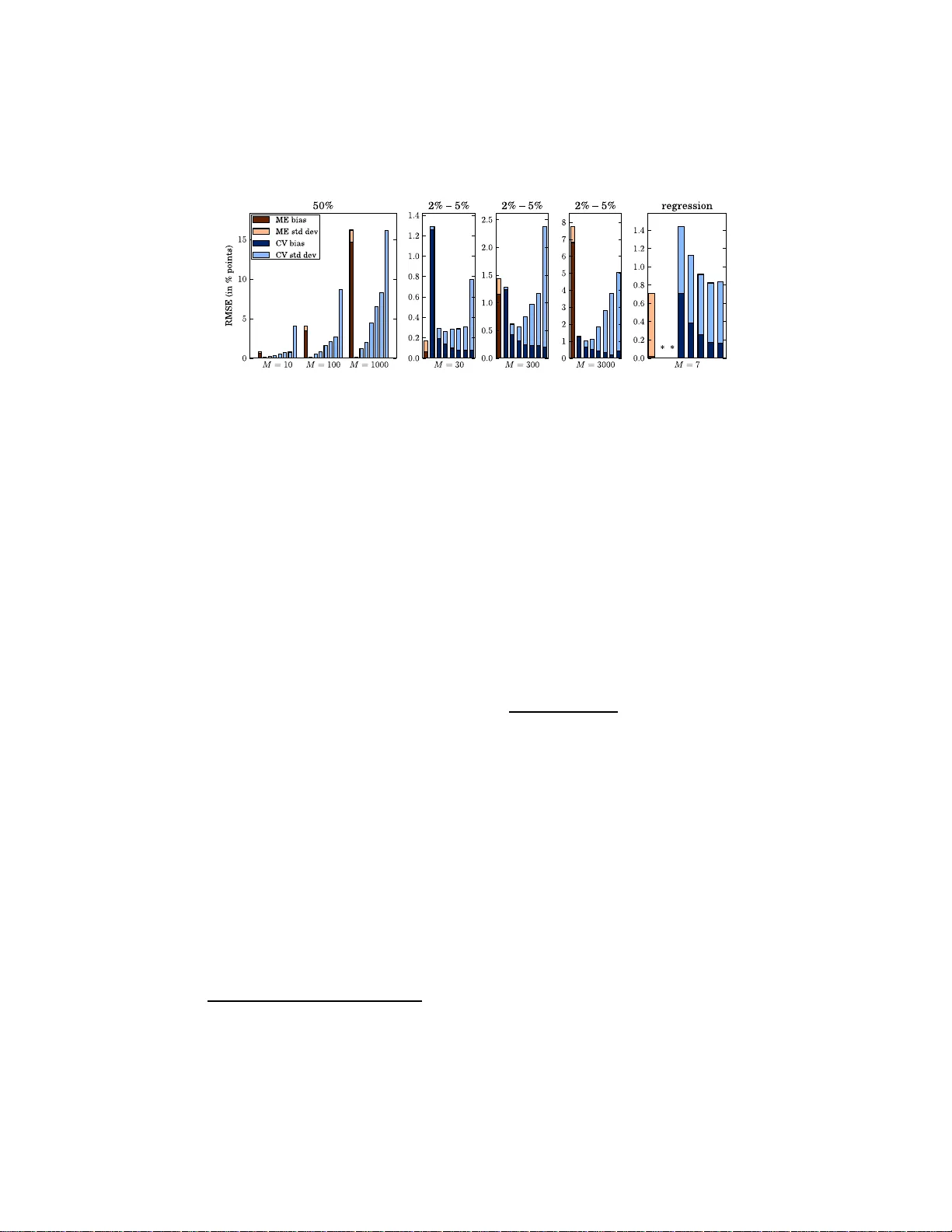
Estimating the Maxim um Exp ected V alue: An Analysis of (Nested) Cross V alidation and the Maxim um Sample Av erage Hado v an Hasselt H.v an.Hass elt@cwi.nl No v em b er 27, 2024 Abstract W e inv estigate the accuracy of th e tw o most common estimators for the maximum e x p ected v alue of a genera l set of random v ariables: a gen- eralization of th e maxim um sample a verage, and cross val idation. No unbiased estimator exists and we sho w th at it is non- trivial to select a goo d estimator without k no wledge ab out th e distributions of the ran- dom v ariables. W e inv estigate and bound the bias and v ariance of t he aforemen tioned estimators and prov e consistency . The v ariance of cross v alidation can b e significantl y reduced, but n ot without risking a la rge bias. The b ias and v ariance of different var iants of cross v alidation are sho wn to b e very problem-depen den t, and a wrong choice can lead to very inaccurate estimates. 1 In tro duction W e often need to estimate the maximum exp e cte d value of a set o f r andom v ar iables (R Vs), when only noisy es timates for each of the v aria bles a re given. 1 F or insta nce, this problem ar ises in optimization in sto chastic decis ion pro cesses and in a lgorithmic ev aluatio n. F orma lly , w e consider a finite set V = { V 1 , . . . , V M } of M ≥ 2 indep endent R Vs with finite means µ 1 , . . . , µ M and v ar iances σ 2 1 , . . . , σ 2 M . W e wan t to find the v alue of µ ∗ ( V ), defined b y µ ∗ ( V ) ≡ max i µ i ≡ max i E { V i } . (1) W e assume the distribution of each V i is unk nown, but a set of noisy samples X is g iven. The question is how b est to use the samples to co nstruct an estimate ˆ µ ∗ ( X ) ≈ µ ∗ ( V ). W e write µ ∗ and ˆ µ ∗ when V a nd X a re clear from the context. 1 Without loss of generality , we assume that we wan t to maximize rather than minimize . 1 It is ea sy to construct consistent estimators, but we ar e also interested in the quality for small sample siz es. The mea n s quared e rror (MSE ) is the most common metric for the quality o f an estimator, but sometimes (the sign o f ) the bias is more imp ortant. Unfortunately , as we discus s in Sectio n 2, no unbiased estimators for µ ∗ exist. A co mmo n es timator is the maximum estimator (ME), which constructs estimates ˆ µ i ≈ µ i and then uses ˆ µ ∗ ≡ ma x i ˆ µ i . When X i ⊂ X contains direct samples for V i , and ˆ µ i is the average of X i , the ME is simply the maxim um sample av era g e. The ME on av era ge ov e restimates µ ∗ . This bias has b een rediscov er ed several times, for ins tance in economics V an den Steen [2004] and decision making Smith and Winkler [20 06]. It can lead to ov eres timation of the per formance of a lgorithms V arma a nd Simon [2 006], Cawley and T alb ot [2010], and p oo r p olicies in reinforcement lear ning a lgorithms v an Ha s selt [2 011a,b]. It is r elated to ove r-fi tting in mo del selection, sele ction bias in sample selection Heckman [19 79] and feature selec tio n Ambroise a nd McLa c hlan [2 002], and the winner’s curse in auctions Cap en et a l. [1 971]. The most commo n alternative to av oid this bias is cr oss validation (CV) Larson [1931], Mosteller and T ukey [19 68 ]. If CV is us ed to construct each ˆ µ i , and ther eafter to estimate µ ∗ (as describ ed in Section 3.2), this is called nested CV o r “double cross” Stone [1 9 74]. Unfortunately , (nested) CV can lead to a large v ar iance. Perhaps surprising ly , we show the abs olute bias of CV can b e larger than the bia s of the ME that we are trying to preven t. How ever, the bias of CV is prov ably negative, which can b e an adv antage. In this paper , we give gener al dis tr ibution-independent bounds for the bias and v ar ia nce of the ME and CV. W e present a new v ar ian t o f CV and show that it is very dep enden t on V which CV estimator is mo st accura te in terms of MSE. Therefore , it is non-trivia l to co nstruct accurate CV estimators witho ut some knowledge ab out the distr ibutions of V . W e discuss why standar d 10-folds CV is o ften not a bad choice fo r mo del selection, but show that in o ther settings other estimator s may be muc h more accura te. W e now discuss tw o motiv ating examples to hig hligh t the practical imp or- tance of this genera l topic. Learning Al gorithms Many learning a lgorithms explicitly maximize noisy v alues to up date their internal par ameters. F o r instance, in r einforcement learn- ing Sutton and Barto [1998] the goal is to find strategies that maximize a r ew ar d signal in a (sequential) decision task. Inaccura te biased estimators for µ ∗ can hav e adverse effects on the sp eed of learning a nd the s tr ategies that ar e lear ned v an Ha s selt [2 011a]. Ev aluation of Algorithms Most ma c hine-lear ning algorithms hav e tunable parameters . Internal p ar ameters , such as the Lagra ngian multipliers of a sup- po rt vector machine (SVM) V apnik [19 95 ], ar e optimized b y the algorithm. Hyp er-p ar ameters , such as the choice of kernel function in a SVM, are often tuned manually or c hosen with domain kno wledge. Other rele v ant choices by 2 the exp erimenter—suc h as which a lgorithms to co nsider a nd the r epresent a tio n of the pr o blem—can be summarized a s meta-p ar ameters . Typically , we ev alua te a s et C o f configurations , wher e each c i ∈ C denotes a specific algor ithm with sp ecific hyper - and meta-para meters. Often, each ev alua tion is noisy , due to (pseudo-)r andomness in the algor ithms or inherent randomness in the problem. The p erformance of c i is then a rando m v ariable V i , and we wan t to construct an estimate ˆ µ ∗ for the best perfo r mance µ ∗ . 2 F or insta nc e , V arma and Simon [2006] no te that the ME res ults in overly- optimistic pr ediction errors and propo se to us e nested CV. They ev alua te an SVM for v a rious hyper -parameters on an a rtificial problem, with an actual er ror of 50%. The estimate by the ME is 41.7% and nested CV results in 54 . 2%. V arma and Simon argue that the latter ex ceeds 50% b ecause nested CV remov es a sa mple from ea c h training set. Howev er, in fact the difference b et ween 5 0 % and 54 . 2% is a demo nstration of a completely different general bias that we discuss in Section 3.2. This bias ha s received very little attention, although—as we will s ho w—it is not in general sma ller than the bia s caused by using the ME . Ov erview In the rest of this section, we discuss r elated work and (notationa l) preliminaries. In Section 2, w e discuss the bias o f estimators in gener al. In Section 3 , we discuss the pr operties of the ME and of CV, including b ounds o n their bias and v ar iance. In Section 4 we discus s concrete s ettings with empirical illustrations. Section 5 co n tains a dis cussion a nd Section 6 co ncludes the pap er. 1.1 Related W ork The b o otstr ap Efron a nd Tibshirani [1993] is a r esampling metho d that can be used to estimate the bias o f an estimator, in o rder to reduce this bia s. Based on this, T ibs hirani and Tibshirani Tibshirani a nd Tibshirani [2 0 09] prop ose an estimator for µ ∗ for model selection in classification. Inevitably—see Section 2—the resulting estimate is s till biased, and it is typically more v a riable that the orig inal estimate. Also s pecifically c o nsidering model selection for class ifiers, Bernau et al. B ernau et al. [2 011] pro pose a smo othed version o f nested CV. The resulting estimator p erforms similar to normal (nested) CV, which in turn is shown to typically be more accurate than the appr o ac h b y Tibshirani and Tibshirani. In this pap er we fo cus o n CV and the ME, whic h are by far the most widely used. The proble m o f estimating µ ∗ is related to the multi-arme d b andit framew o rk Robbins [1 952], Berry and F ristedt [1985], where the goal is to find the identity of the action with the maximum exp ected v alue r a ther than its value . The fo cus in the liter ature on multi-armed bandits is often on how b est to collec t samples. In contrast, in this pap er we assume that a set of samples is given. A discussion on how b est to co llect samples to minimize the bias o r MSE is o utside 2 Sometimes w e are more in terested in the configuration that optimizes the p er formance than in the resulting p erformance, but often the p erformance itself i s at least as imp ortan t. In part, this depends on whether the fo cus of the r esearc h is on the algorithms or on the problem. 3 the sco pe o f this paper , although w e do note that minimizing online regret Lai and Robbins [1 985], Auer et al. [2 002] does not neces s arily corresp ond to minimizing the online MSE o f the estimator. 1.2 Preliminaries The measurable doma in of V i is X i , and f i : X i → R deno tes its probability density function (PDF), such that µ i = R X i x f i ( x ) dx . F or conciseness, we assume X i = R . W e assume these PDFs f i are unknown and ther efore µ ∗ = max i µ i can not be found analytica lly . W e write ˆ µ i ( X ) for an es timator for µ i based on a sa mple set X . Similarly , ˆ µ ∗ ( X ) is an estimator for µ ∗ . W e write ˆ µ i and ˆ µ ∗ when X is clear from the context. If X i ⊂ X is a s et of unbiased sa mples for V i , ˆ µ i might b e the sample av erag e. In that cas e, ˆ µ i is unbiased for µ i . In gener al, ˆ µ i can be biased for µ i . As discussed in the next section, no g eneral un bia s ed estimator for µ ∗ exists, even if a ll ˆ µ i are unbiased. The following de finitio ns will b e useful b elow, when stating ne c e ssary a nd sufficient co nditions for a strictly p o sitiv e o r a strictly nega tiv e bia s . The s et of optimal indices for R Vs V is defined as O ( V ) ≡ { i | µ i = µ ∗ } . (2) The set of maximal indices for samples X is defined a s M ( X ) ≡  i     ˆ µ i ( X ) = max j ˆ µ j ( X )  . (3) An estimator is called optimal or ma ximal whenever its index is optima l o r maximal, resp ectiv ely . Note that optimal estimators are not necessar ily maximal and maximal es timators are not necessarily optimal. 2 The Bias of an Estimator Let V be a function space containing all admissible sets o f M R Vs. W e might know V , but not the precise iden tity of V ∈ V . F or instance, V may b e the set of all se ts o f M normal R Vs with finite moments. Let p : V → R b e a P DF ov er V . The exp ected MSE of an es timator ˆ µ ∗ is equal to Z V p ( V ) Z X P ( X | V ) ( ˆ µ ∗ ( X ) − µ ∗ ) 2 dX dV , (4) In a n y given concrete s etting, ther e is a sing le unknown set V . Ther efore, p do es not exist ‘in the world’. Ra ther, p might mo del our pr ior b elief ab out which sets V ar e likely in a given setting, or it might s pecify the V for w hich we would like an estimator to p erform well. The MSE consists o f v ar iance and bia s. T o rea son in some generality ab out which estimators are go o d in pr actice, we discuss the non-existenc e of unbiase d estimators and the dir e ct ion of t he bias . 4 Non-Existence of Un biased Estimators By definition, ˆ µ ∗ is a general un bias ed estima tor (GUE) for V if and o nly if ∀ V ∈ V : E { ˆ µ ∗ | V } = µ ∗ . (5) Unfortunately , for most V of in terest no suc h estimator exists. F or instance, Blument hal and Cohen [196 8 ] show no GUE exists for tw o nor mal distributions and Dhariyal et al. [198 5 ] pro ved this for arbitrar y M ≥ 2 a nd fo r more gen- eral distributions, including the ex ponential family . Esse ntially , the arg umen t is that a r e asonable estimator for µ ∗ depe nds smo othly on the v alues o f the samples, wherea s the real v a lue µ ∗ is a piece-w is e linea r function with a dis - contin uous deriv ative. W e can not know the loc a tion o f these discontin uities without knowing the actual maximum. Note that (5) is alr eady false if V contains only a single set of v ariables for which ˆ µ ∗ is biased. How ever, bias alone do es not tell us everything, a nd a low bias do es not necessarily imply a s mall ex pected MSE. The Directio n of the Bias In s ome cases, the direction of the bias is very impo rtan t. Supp ose we test a n a lgorithm fo r v ar ious hyper -parameters a nd observe that the b est p erformance is b etter than some bas eline. If w e simply use the hig he s t test result, it can not b e co ncluded tha t the algo rithm can r e ally structurally outp erform the baseline for any of the sp ecific hyper - parameters. Although this may sound trivial, it is co mmon in practice: when we manually tune hype r - or meta-para meters on a problem and use the b est result, we are using ma x i ˆ µ i , which has no n- negative bias . It is hard to av oid optimizing on meta-parameter s: these include the very (prop erties o f the) pr o blem we test the algorithm on. The practical implication of this po sitiv e bias is tha t the algo rithm will disapp oin t in future ev alua tions on similar (rea l-w or ld) problems. In con tra st, if we use an es timator with non-p ositive bias and our es timate is hig her than the baseline, we can have muc h more confidence that the alg orithm can reach that pe rformance c o nsisten tly with a prop erly tuned h yp er-par a meter. This is similar to the co nsiderations about ov er fitting in mo del sele c tion, where CV is most often used. W e prov e below that CV indeed has non-p ositive bias, and can therefor e a void overestimations of µ ∗ . As another exa mple, the perfor mance o f most machin e- learning a lgorithms improv es when more data is a v ailable. When the data c ollection is exp ensiv e it is useful to pr edict how an alg orithm p erforms when more da ta is av ailable, b efore actually collecting this da ta. An overestimation of the future p erforma nce can lead to a misallo cation o f resour ces, since the collected data may b e less useful than pr e dicted. An under estimation means we may b e to o p essimistic, and to o often decide not to co llect more data. Whether or not the false p ositives a r e more important than the false nega tiv es depends crucially on specifics of the setting. 5 3 Estimators for the Maxim um Exp ected V al ue In this s ection, we discuss the ME and CV estimators for µ ∗ in deta il. W e b ound the biases and v ariance s of all estimator s, discuss s imila rities and co n trasts, a nd prov e consistency . W e in tro duce a low-v ariance v ariant o f CV. W e give necess ary and sufficient conditions for non-zero biases to o ccur for a ll e s timators, a nd per haps sur prisingly we show that there ar e settings in which the negative bias of all v ar ia n ts of CV is lar ger in size than the p ositive bia s o f ME. All pro ofs are given in an app endix and the end of this pap er. 3.1 The Maxim um-Estimator E stimator The maximum-estimator (ME) estimator for µ ∗ is ˆ µ ME ∗ ( X ) ≡ max i ˆ µ i ( X ) , (6) where ˆ µ i is a (p ossibly bias ed) estimator fo r µ i . B ecause it is conceptually simple a nd eas y to implemen t, the ME estimator is often use d in pra ctice. The theorem b elow prov es its bias is no n-negative and gives necessary a nd sufficient conditions for a strictly p ositive bias. The theo rem is stronger and more gener al than some similar e arlier theorems. F or instance, Smith a nd Winkler [2006] do not consider the p ossibility of m ultiple optimal v aria bles, and do not discuss necessity of the conditions for a strictly positive bias. Theorem 1. F or any given set V , M ≥ 1 and unbiase d estimators ˆ µ i , E { ˆ µ i | V } = µ i , E { ˆ µ ME ∗ | V } ≥ µ ∗ , with e quality if and only if al l optimal indic es ar e maximal with pr ob ability one. Theorem 1 implies a low er b ound of z e r o for the bias of the ME. An upp er bo und for ar bitrary means a nd v ar iances is given by Aven [198 5]: Bias( ˆ µ ME ∗ ) ≤ v u u t M − 1 M M X i V ar ( ˆ µ i ) , (7) which is tight when the estimato r s ar e iid [Arno ld a nd Gro eneveld , 19 79], indi- cating that iid v a riables a re a worst-case s etting. W e do not know of pr evious work that b ounds the v ar iance, which we discuss next. Theorem 2. The varianc e of t he ME estimator is b ounde d by V ar ( ˆ µ ME ∗ ) ≤ P M i =1 V ar ( ˆ µ i ) . Theorem 2 a nd b ound (7) imply that ˆ µ ME ∗ is consis ten t for µ ∗ whenever each ˆ µ i is co nsisten t for µ i and that MSE ( ˆ µ ME ∗ ) < 2 P M i =1 V ar ( ˆ µ i ). 6 3.2 The Cross-V alidation E stimator In general, µ ∗ can b e considered to b e a weigh ted av erag e of the means of all optimal v a riables: µ ∗ = 1 |O ( V ) | P M i =1 I ( i ∈ O ( V )) µ i , where I is the indicator function. W e do not know O ( V ) and µ i , but with s ample sets A, B we can approximate these w ith M ( A ) a nd ˆ µ i ( B ) to obtain µ ∗ ≈ ˆ µ ∗ ≡ 1 |M ( A ) | M X i =1 I ( i ∈ M ( A )) ˆ µ i ( B ) . (8) If A = B = X , this reduce s to ˆ µ ME ∗ . How ever, suppo s e that A and B a re independent. This idea leads to cr oss-validation (CV) estimators. Of c o urse, CV itself is not new. How ever, it seems to b e less well-kno wn how prop erties of the pro ble m affect the accura cy and that CV c a n b e quite biased. W e split each X into K disjoin t sets X k and define ˆ µ k i ≡ ˆ µ i ( X k ). F or instance, ˆ µ k i might b e the sample av er age o f X k i . W e consider tw o different CV estimators. In b oth metho ds, for each k ∈ { 1 , . . . , K } we construct a n ar gument set ˆ a k and a value set ˆ v k . L ow-bias cr oss validation (LBCV) is the ‘standard’ CV estimator, where K − 1 sets ar e us e d to build the a rgumen t set ˆ a k (the mo del), a nd the remaining set is used to determine its v alue: ˆ a k i ≡ ˆ µ i ( X \ X k ) and ˆ v k i ≡ ˆ µ i ( X k ) ≡ ˆ µ k i . L ow-varianc e cr oss validation (L VCV) reverses the definitions fo r ˆ a k and ˆ v k : ˆ a k i ≡ ˆ µ ( X k i ) ≡ ˆ µ k i and ˆ v k i ≡ ˆ µ ( X i \ X k i ) . W e do not know of an y prev ious w ork that discusses this v a riant . How ever, its lo wer v aria nce can sometimes result in muc h low er MSEs tha n obtained by LBCV. F or b oth LBCV and L V CV, if ˆ µ i ( X ) is the sample av era ge of X i and all samples are unbiased, then E { ˆ a k i } = E { ˆ v k i } = µ i . F or either approach, M k is the set of indices that maximize the ar gumen t vector. F or LB CV this implies M k = M ( X \ X k ) and for L V CV this im- plies M k = M ( X k ). W e find the v alue of these indices with the v alue vector, resulting in ˆ µ k ∗ ≡ 1 |M k | X i ∈M k ˆ v k i . (9) W e then av erag e over all K sets: ˆ µ CV ∗ ≡ 1 K K X k =1 ˆ µ k ∗ = 1 K K X k =1 1 |M k | M X i ∈M k ˆ v k i , ( 1 0) where either ˆ µ CV ∗ = ˆ µ LBCV ∗ or ˆ µ CV ∗ = ˆ µ L VCV ∗ , dep ending o n the definitions of ˆ a k i and ˆ v k i . 7 The cons tr uction of ˆ µ k ∗ per forms the appr oximation: ˆ v k i ≈ ˆ v k i ∗ ≈ µ i ∗ ≡ µ ∗ , where i ∈ M k and i ∗ ∈ O . The first approximation results from using M k to approximate O and is the ma in source of bias. The seco nd approximation results from the v ar iance of ˆ v k . F or la r ge enough X , K can be tr eated as a parameter that trades off bias and v ariance. F or LBCV la rger K implies less bias a nd more v ariance, while for L V CV it implies more bia s a nd less v arianc e . F or K = 2, LB CV and L VCV are equiv alent. If K > 2, L VCV is mo r e biased but les s v ar ia ble than LBCV, since M k is then base d o n few er sa mples while ˆ v k i is based on more s amples. When ∀ i : | X i | = K for LBCV, ˆ v k i is based o n a single sample, r esulting in a large v a riance. This v aria n t is co mmo nly known as le ave-one-out CV. When ∀ i : | X i | = K for L V CV, ˆ a k i is based on a single sa mple, p oten tially r esulting in large bias due to larg e probabilities of selecting s ub-optimal indices. The bias of CV for µ ∗ has received comparatively little attention. Sometimes the bias is mentioned without explanatio n [Kohavi , 1995], and sometimes it is even claimed that CV is unbiased [Mannor et al., 2007]. Often, any o bserved bias is attributed to the fact that ˆ a k can b e biased whe n it based on K − 1 K | X | rather than | X | samples [V ar ma and Simon, 2006]. This ca n b e a factor, but the bia s induced by using M k for O is often at least as imp ortant, as will b e demonstrated below. Some confusion seems to ar is e from the fact tha t ˆ v k i is often un biased for µ i . Unfortunately , this do es not imply that ˆ µ CV ∗ is un biased for µ ∗ . Next, we prov e that CV es timators can have a negative bias even if ˆ a and ˆ v are un biased, and we give neces s ary and sufficien t conditions for a strictly negative bias. Theorem 3. If E  ˆ µ k i   V  = µ i is u nbiase d then E { ˆ µ CV ∗ | V } ≤ µ ∗ is n e gatively biase d, with a strict ine quality if and only if ther e is a non-zer o pr ob ability that any non-optimal index is maximal. The theorem sho ws that ˆ µ L VCV ∗ and ˆ µ LBCV ∗ on a verage underes timate µ ∗ if and o nly if there is a non-zero probability that i ∈ M k ( X ) for some i / ∈ O ( V ). A prominent case in which this do es not hold is when all v ariables hav e the same mean, since then i ∈ O ( V ) for all i . Int er estingly , this implies that CV is un bias ed when the V i ∈ V ar e iid, which is a worst case for the ME. Theorem 3 implies that the bias of CV is b ound from a bov e by zero. W e conjecture the bias is b ound fro m b elo w a s follows. Conjecture 1. L et E  ˆ µ k i   V  = µ i . Then Bias ( ˆ µ CV ∗ ) > − 1 K K X k =1 v u u t M X i =1 V ar  ˆ a k i  . W e do not prov e this conjecture here in full generality , but there is a proo f for M = 2 in the app endix. It makes in tuitive sense that the bias of ˆ µ CV ∗ depe nds only on the v aria nces V a r  ˆ a k i  if e a c h ˆ µ k i is un biased. The bias o f the 8 CV estimators is una ffected by the fact that ˆ µ CV ∗ av erag es over K estimators ˆ µ k ∗ , but K do es affect the bias by regulating how man y samples ar e used for each ˆ a k i . As mentioned ear lier, for L VCV la r ger a K implies a higher bia s since then ˆ a k i is mor e v ariable, w hile for LBCV a larger K implies a lower bias since then ˆ a k i is less v aria ble . Although CV is known for lo w bias and high v a riance, the next theo r em shows its a bs olute bias is not necessa rily smaller than the absolute bias of the ME. Theorem 4. Ther e exist V and N = | X | such t hat | Bias ( ˆ µ CV ∗ | N ) | > | Bias ( ˆ µ ME ∗ | N ) | for any K and for any variant of CV. Two different ex p eriments in Section 4 prov e this theorem, since there ev en the nega tiv e bias of leave-one-out LB C V is large r in size than the pos itive bias of ME. Theorem 5. The varianc e of ˆ µ LBCV ∗ is b ounde d by V ar ( ˆ µ LBCV ∗ ) ≤ 1 K 2 K X k =1 M X i =1 V ar  ˆ µ k i  . If each ˆ µ k i is unbiased, the v a riance of L V CV is necessar ily smalle r than that of LBCV a nd the same b ound applies trivially to ˆ µ L VCV ∗ . Corollary 1. If ˆ µ i is the sample aver age of X i and | X k i | = | X i | /K for al l k , then V ar ( ˆ µ CV ∗ ) ≤ P M i =1 V ar ( ˆ µ i ) for b oth LBCV and L VCV. Conjecture 1 and Theor em 5 imply that CV is co ns isten t if each ˆ µ i is con- sistent and K is fixed (or slo wly increas ing, see als o Shao [199 3 ]), a nd that MSE( ˆ µ CV ∗ ) ≤ 2 P M i =1 V ar ( ˆ µ i ). 4 Concrete Illustrations T o illustrate that it is non-trivial to s elect a n a c c urate estimato r, we discuss some concr ete examples. 4.1 Multi-Armed Bandits for In ter net Ads The framework of multi-armed bandits c an b e us e d to o ptimize which ad is shown on a website [Langfor d et a l., 20 08, Strehl et al., 2010]. Consider M ads with unknown fixed exp ected retur ns p er visito r µ i . Bandit algo rithm can b e used to ba lance exploration and ex ploitation to optimize the online return p er visitor, which conv erges to µ ∗ . How ever, quick accura te estimates of µ ∗ can b e impo rtan t, fo r instance to ba se future in vestment s o n. Additionally , pla c ing any ad may induce some cos t c , so we may wan t to kno w q uickly whether µ ∗ > c . F or simplicity , ass ume ea c h ad has the same r eturn per click, such that only the click ra te matters and e a c h V i can b e mo deled with a B ernoulli v a riable with 9 Figure 1 : The MSE for ˆ µ ME ∗ , ˆ µ LBCV ∗ and ˆ µ L VCV ∗ for different settings, av eraged ov er 2,000 exp eriments. T he left-most bar is alwa ys ˆ µ ME ∗ . The other bars are , from left to righ t, leave-one-out L VCV, 10 -folds L V CV, 5-folds L VCV, 2 - folds CV, 5-fo lds LBCV, 1 0-folds LB C V and leav e-one-out LBCV. Note that 2-folds L V CV is eq uiv alent to 2-folds LBCV, which a re therefo r e not shown separ ately . mean µ i and v ar iance (1 − µ i ) µ i . In o ur first ex periment, there are N = 10 0 , 0 00 visitors, M = 1 0, M = 100 or M = 10 00 ads, a nd ∀ i : µ i = 0 . 5. All ads ar e shown equally o ften, such that ∀ i : N i = N / M . B e cause all means are equal, Theorem 3 implies that CV estimator s are un biased; their MSE dep ends solely on the v aria nc e . In the second—mor e rea lis tic—setting, the M mea n click rates are distributed evenly b et ween 0 . 02 and 0 . 0 5, there are N = 300 , 0 00 visito rs, and M = 30, M = 300 , or M = 3000 ads. The results are s hown in the first four plots in Figure 1. W e show the r oot MSE (RMSE), such that the units ar e p ercent a g e p oints. Within the RMSEs, the con tributions of the bias a nd the v ar iance are sho wn. No te that MSE = bias 2 + v ar iance, and therefo r e RMSE = p bias 2 + v aria nce 6 = bias + std dev . This implies that the depicted contributions of bia s and v aria nce to the RMSE are no t in general exactly equal to the bias a nd standa rd deviation, but this depiction do es allow us to see direc tly how many p ercentage p oin ts of err or a re caused by bia s a nd by v ariance. In the first setting (left plot) CV is indeed unb ia sed. Leav e-one- out L V CV has the low est v a riance of a ll CV methods—it is barely visible—which implies it has the smalles t MSE. F or M = 1000 ads, the huge bias o f the ME causes it to ov eres timate the a ctual ma x imal click rate by more than 15%. In the second setting (middle thr ee plots), there is a clear tra de-off in CV: L V CV with la rge K has larg e bias a nd small v ar iance, wher eas LBCV w ith lar ge K has sma ll bias and larg e v aria nce. 3 The bias of the CV estimators is clearly impo rtan t, even though each ˆ µ k i is unbiased. Even for leave-one-out LB CV the bias is non-neg ligible: for M = 30 its bias is lar ger than the bias of the ME. Int er estingly , when M increases (and the num be r of sa mples p e r ad decreas es 3 Sometimes the bias of LBCV seems to i ncrease slightly for higher K . These ar e noise- related artifacts. 10 corres p ondingly) the er ror for leave-one-out L V CV sta ys virtua lly unc hang ed, at approximately 1.3%. Since the error o f a ll other estimators increases with increasing M , this implies that le ave-one-out L V CV g oes from b eing by far the least accura te for M = 30 to almost the most accura te for M = 3000 . In contrast, the ME go es from b eing the mo st accur ate for M = 30 to the lea st accurate for M = 3 0 00. The reason is that for incr easing M , the v a riables a re relatively more similar to iid v ariables, which is a b est case for L VCV and a worst case for the ME. In all three cases, 10 - and 5- folds L V CV a re a go o d choice. 4.2 Ev aluation of Algorithms W e now consider a regre s sion problem. The goa l is to fit p olynomials on no isy samples fro m a function r ( y ) = 4(sin( y ) + sin(2 y )). Let X = { ( y , r ( y ) + ω ) | y ∈ Y } denote a no isy da ta set for inputs Y , where ω is zero -mean Gaussia n noise with v aria nce σ 2 ω = 4. Let p i denote a po lynomial of deg ree i , of which the co efficien ts a re fitted with lea st-squares on X . Let Y = { 0 , 0 . 0 5 , . . . , 3 . 9 5 , 4 } be 8 1 equidista n t inputs. W e wan t to maximize the negative MSE. The lowest exp ected MSE of fitting each p i on 81 samples and testing on an indep e ndent test s et of 81 sa mples is obtained at 4 . 34 for i = 5, which implies µ ∗ = µ 5 = − 4 . 34 . W e construct 1,00 0 independent noisy sets X = { ( y , r ( y ) + ω ) | y ∈ Y } . F o r each X , we conduct the follo wing experiment. F or any given Z ⊆ X , ˆ µ i is defined by a n inner CV loop as fo llows. F or each z ∈ Z , we fit p i on Z \ { z } and test the e r ror on z to obtain an er r or e i ( z ). W e average these err ors to obtain: ˆ µ i ( Z ) = 1 | Z | P z ∈ Z e i ( z ). This implies ˆ µ i is biased, since p i is fitted on | Z | − 1 < 81 sa mples. F o r the ME, ˆ µ ME ∗ = max i ˆ µ i ( X ) which means | Z | = 8 0 samples are used to fit each p i . F or LBCV, ˆ a k i = ˆ µ i ( X \ X k ) which means | Z | = K − 1 K 81. F or L V CV, ˆ a k i = ˆ µ i ( X k ), which means | Z | = 1 K 81. Since | Z | can then be m uch sma ller than 81 , L VCV can b e significantly biased. W e consider K ∈ { 2 , 3 , 9 , 81 } . When K = 81 , LBCV is also known as n este d le ave-one-out CV . Fig ure 1 (right plo t) shows the r esults. L V CV is not shown for K = 8 1 and K = 9: L V CV with K = 81 is meaning- less, since one cannot fit a p olynomial o n a sing le p oin t. The MSE for K = 9 is hu g e . In s harp co n trast with the previo us s ettings, L V CV fares p o orly—even in terms of v aria nc e —a nd lea ve-one-out LBCV is the b est CV estimato r. How ever, int er estingly the ME is mo re accura te than all CV estimator s, and e v en the size of its bia s (0 . 0 18) is muc h smaller than that of n - fold LBCV ( − 0 . 190). 5 Discussion Our results show that it is hard to cho ose an estimato r that is g oo d in general. Unfortunately , the b est choice in one s etting can be the worst choice in ano ther. A p o orly chosen CV estimato r can be far less accura te than the ME. T his do es not imply tha t we sugges t using the ME; it is often very biased. 11 A p oten tial adv a n tage of CV es tima to rs in some settings is a guara n teed non-p ositive bias. This can b e desirable even if the estimator is less accu- rate. How ever, in our r esults the recommendatio n to alwa ys use 10- folds LBCV [Kohavi , 1995] seems unfounded. When each ˆ µ i is unbiased and esp ecially when M is larg e, L V CV often p erforms muc h b etter. On the o ther hand, when each estimator ˆ µ i has a bia s that decreases with the num b er of samples, the bias of L V CV can become pr ohibitiv ely lar ge, as illustr ated in the regression setting. This ex plains why 10- folds L B CV is often not a bad choice for mo del selection, as long as M is fairly small and ˆ µ i is fairly biased. Howev er, note that 5- and 10-folds LBCV w ere the most accur ate estimator in n one of o ur e x periments. As a general r ecommendation, it may b e go od to try both the ME and o ne or more CV estimato rs. If the estimates ar e close together, this indicates they are more likely to be accura te. A lthoug h the true maximum ex pected v alue will o ften lie b etw e en the es timate by the ME a nd those by CV, one should not simply av era ge these es tima tes : as we have shown that for instance the ME can be very bia sed in s ome s ettings, and hardly biased in others. F urthermor e, the po ten tially ex cessive v arianc e o f some v a riant s of LBCV implies that in some cases its estimate ma y itse lf b e an ov ere stimation, which is why we reco mmend to include L VCV in the analysis. Alternativ e estimators Of cours e, there ar e p ossible alterna tiv es to the es- timators we discussed. First, one can consider using the ma xim um of some low er confidence b ounds on the individual v alue estimates. Although this does counter the o verestimation of ME, it can not b e guaranteed tha t this do es no t lead to an underestimatio n in its place. F urthermor e, it is non-trivial to select a go od confidence in terv al, a nd the res ulting estimate will typically b e m uch more v ariable than the ME. Second, for mo del-selection there exist cr iter ia such as AIC [Ak aike, 19 74] and BIC [Sch warz , 1978] that use a p enalt y term based on the num b er of pa ram- eters in the mo del. Obviously , s uch p enalties are only useful when comparing homomorphic models with differen t n umbers of parameters, and therefore do not apply to the more genera l setting we co ns ider in this pa per. F ur ther more, the main purp ose of these cr iteria is not to giv e an accura te estimate of the exp ected v a lue o f the b est mo del, but to increase the probability o f selecting it. These goa ls are related, but unfortuna tely not equiv alent. Finally , o ne can estimate b elief distributions ˆ F i for the lo catio n of each µ i , for instance with Bayesian inference. With these distributions, we can estimate µ ∗ . This appro ac h is less general, since it r e quires pr io r knowledge ab out V , but then it doe s seem r easonable. The probability that the maximum mean is smaller than some x is eq ua l to the pro babilit y that all mea ns are smalle r than x . Therefore, its CDF is ˆ F max ( x ) = Q M i =1 ˆ F i ( x ), which w e ca n use to estimate µ ∗ . The resulting Bay esia n es tima to r (BE) is ˆ µ BE ∗ = Z ∞ −∞ x M X i =1 ˆ f i ( x ) Y j 6 = i ˆ F j ( x ) dx , 12 where ˆ f i ( x ) = d dx ˆ F i ( x ). T o sho w a p erhaps counter-int uitive result fro m this approach, we dis c uss a small example. Consider tw o Bernoulli v a riables. W e consider all means eq ually likely and use a uniform prio r Beta dis tribution, with parameters α = β = 1. Supp ose µ 1 = µ 2 = 0 . 5. W e dra w tw o samples fro m each v a r iable. The exp ected estimate for the ME is 21 32 , for a bia s of 5 32 ≈ 0 . 1 56. CV is unbiased, since the means a r e equal. F o r the BE ˆ F i ( x ) is 1 − (1 − x ) 3 , 3 x 2 − 2 x 3 or x 3 , dep ending on how many samples for V i are equa l to one. Its exp ected v alue is then E  ˆ µ BE ∗  = 737 1120 ≈ 0 . 658. Note that the p ositive bias is even higher than the bias of the ME. This is due to our uniform prior : if the prior on the individual v aria bles is uniform, this implies the prio r for the maximum exp ected v alue is ne g ativ ely skew ed, a nd its ex p ected v alue is incr eased. The effect is already appar en t with tw o v ar iables, but it increases further with the nu mber of v a riables due to the s hape of ˆ F max ( x ) = Q M i =1 ˆ F i ( x ). 6 Conclusion W e analyzed the bia s a nd v ar iance of the tw o most common estimator s for the maximum e x pected v alue of a set of random v ariables . The maximum estimate results in non-ne g ativ e bia s. The common alternative of cr oss valida tion (CV) has non-p ositive bias, which can b e preferable. Unfortunately , the accurac ie s of different v ariants of CV are very dep enden t on the s e tting; an uninfor med choice can result in e x tremely inaccurate es timates. No general r ule—e.g., alwa ys use 10-fold CV—is alw ays o ptimal. App endix Pr o of of The or em 1. F or co nciseness, we leave V and X implicit. Let j ∈ O be an ar bitrary optimal index, and define event A j ≡ ( j ∈ M ) to be true if and only if j is max imal. W e ca n write µ ∗ = P ( A j ) E { ˆ µ j | A j } + P ( ¬ A j ) E { ˆ µ j | ¬ A j } . Note: E { ˆ µ j | A j } = E { ˆ µ ME ∗ | A j } and E { ˆ µ j | ¬ A j } < E { ˆ µ ME ∗ | ¬ A j } . Ther e fo re, µ ∗ ≤ E { ˆ µ ME ∗ } , with eq ualit y if and only if P ( ¬ A j ) = 0 for all j ∈ O . Pr o of of The or em 2. Let A and B be independent sets of R Vs with E { A i } = E { B i } and E  A 2 i  = E  B 2 i  . Define C ( i ) ≡ ( A \ A i ) ∪ { B i } = { A 1 , . . . , A i − 1 , B i , A i +1 , . . . , A M } . The Efron-Stein inequality [Efron and Stein, 19 81] states that for any g : R M → R : V ar ( g ( A )) ≤ 1 2 M X i =1 E   g ( A ) − g ( C ( i ) )  2  . 13 Let A and B be indep enden t instantiations of ˆ µ and let g ( A ) = max i A i for any A . W e derive V ar ( ˆ µ ME ∗ ) ≤ 1 2 M X i =1 E (  max j A j − max j C ( i ) j  2 ) ≤ 1 2 M X i =1 E n ( A i − B i ) 2 o = M X i =1 V ar ( ˆ µ i ) . Pr o of of The or em 3. Let w k i ≡ E  I ( i ∈ M k ) / |M k |  . Then E  ˆ µ k ∗  = P M i w k i µ i ≤ µ ∗ , b ecause M k and ˆ v k i are indep endent , P M i w k i = 1 and E  ˆ v k i  = µ i . No te that w k i > 0 if and o nly if P  i ∈ M k  > 0. Ther efore, E  ˆ µ k ∗  < µ ∗ if and only if there ex ists a i / ∈ O such that P  i ∈ M k  > 0. Pr o of of Conje ctu r e 1 for M = 2 . Ass ume without loss o f generality that µ 1 = µ ∗ . The assumption E  ˆ µ k i  = µ i implies that E  ˆ v k i  = µ i . Then, Bias  ˆ µ k ∗  = E  I (2 ∈ M k ) |M k |  ( µ 2 − µ 1 ) ≥ P  2 ∈ M k  ( µ 2 − µ 1 ) = P  ˆ a k 2 ≥ ˆ a k 1  ( µ 2 − µ 1 ) ≥  V ar  ˆ a k 1  + V ar  ˆ a k 2  ( µ 2 − µ 1 ) V ar  ˆ a k 1  + V ar  ˆ a k 2  + ( µ 1 − µ 2 ) 2 ≥ − 1 2 q V ar  ˆ a k 1  + V ar  ˆ a k 2  , where the second inequality follows from Cantelli’s inequality , and the thir d inequality is the result of minimizing for µ 2 − µ 1 . F r om this, it follows that for M = 2 Bias( ˆ µ CV ∗ ) ≤ − 1 2 K K X k =1 v u u t 2 X i =1 V ar  ˆ a k i  , which is a fa ctor 1 2 tighter than the genera l b ound in the conjecture. Pr o of of The or em 5. W e apply definition (10) a nd use P K k =1 ˆ v k i = P K k =1 ˆ µ k i to derive V ar   1 K K X k =1 1 |M k | M X i ∈M k ˆ v k i   ≤ V ar 1 K K X k =1 M X i =1 ˆ v k i ! ≤ 1 K 2 K X k =1 M X i =1 V ar  ˆ µ k i  . Pr o of of Cor ol lary 1. Apply Theorem 5 with V ar  ˆ µ k i  = σ 2 i / | X k i | = K σ 2 i / | X i | = K V ar ( ˆ µ i ) 14 References H. Ak aike. A new lo ok at the statistical mo del ident ifica tio n. IEEE T r ansactions on Automatic Contr ol , 19 (6):716–723 , 197 4. C. Ambroise a nd G. McLac hla n. Selectio n bias in gene extraction on the basis of microarray gene-expres sion data. Pr o c e e dings of the National A c ademy of Scienc es , 99(10):65 62, 2 0 02. B. C. Arnold and R. A. Gro eneveld. Bounds on exp ectations o f linea r systematic statistics based on dep enden t samples. The Annals of St atistics , 7(1):22 0–223, 1979. P . Auer, N. Cesa -Bianchi, and P . Fischer. Finite-time analysis of the m ultiar med bandit pro blem. Mac hine le arning , 47(2):23 5 –256, 2 002. T. Aven. Upper (lo wer) b ounds on the mea n of the maximum (minimum) of a num b er of random v a riables. Journ al of applie d pr ob ability , 22(3):7 2 3–728, 1985. C. Berna u, T. Augustin, and A.-L. Boules teix. Corr ecting the optimally selected resampling-ba sed error rate: A smo oth ana ly tical alternative to nested cros s - v alidatio n, 20 11. D. A. Berry and B. F ristedt. Bandit Pr oblems: se quent ial al lo c ation of exp eri- ments . Chapman a nd Hall, London/New Y ork, 19 85. S. Blumenthal and A. Cohen. E stimation o f the larger o f tw o no rmal means. Journal of the Ameri c an Statist ic al Asso ciation , pa ges 86 1–876, 19 68. E. Cap en, R. Clapp, a nd T. Campb ell. B idding in high risk situations. J ournal of Petr oleum T e chnolo gy , 23:6 41–653, 1971 . G. Cawley and N. T alb ot. On ov er-fitting in model selection and subsequen t selection bia s in pe rformance ev aluation. The Jour n al of Machi ne L e arning R ese ar ch , 11:2079– 2107, 201 0. I. Dhar iy al, D. Sharma, and K . Krishnamo orthy . Nonexistence of unbiased estimators of ordered parameter s. S tatistics , 16(1):89 –95, 1985. B. Efro n a nd C. Stein. The jac kk nife estima te of v ar iance. The A nn als of Statistics , 9(3):58 6–596, 198 1. B. E fron and R. Tibshira ni. An intr o duct ion to the b o otst ra p , volume 5 7. Chap- man & Hall/ C RC, 1993 . J. Heckman. Sample selectio n bias a s a s pecification er ror. Ec onometric a: Journal of the e c onometric so ciety , pa ges 15 3–161, 1 979. 15 R. Kohavi. A study o f cross-v alidation and bo otstra p for accur acy estimation and mo del selection. In C. S. Mellish, editor, Pr o c e e dings of t he F ourte enth International J oint Confer enc e on Artificial Int el lig enc e (IJCAI-95) , pa ges 1137– 1145, Sa n Mateo, 19 95. Morga n Kaufmann. T. Lai and H. Robbins . Asymptotically efficient adaptive allo cation rules . A d- vanc es in Applie d Mathematics , 6 (1):4 – 22, 1985. J. Lang ford, A. Strehl, and J. W or tman. Ex ploration scav eng ing . In Pr o c e e dings of the 25 th international c onfer enc e on Machi ne le arning (ICML-08) , pages 528–5 35. ACM, 200 8. S. Lar son. The shr ink age of the co efficien t o f multiple corr elation. J ournal of Educ ational Psycholo gy , 22 (1 ):45, 19 31. S. Mannor, D. Simester, P . Sun, a nd J. N. Tsitsik lis . Bias a nd v ar iance a ppr o x- imation in v alue function estimates. Management Scienc e , 53 (2):308–322 , 2007. F. Mo s teller and J. W. T ukey . Data analys is, including statistics. In G. Lindzey and E. Aro nson, editor s, Handb o ok of S o cial Psycholo gy, V ol. 2 . Addison- W esley , 196 8. H. Robbins. Some asp ects of the sequential design of exp eriments. Bul l. Amer. Math. So c , 58(5):527 –535, 1 9 52. G. Sch warz. Estimating the dimension of a mo del. The annals of statistics , 6 (2):461–4 64, 1 978. J. Shao. Linea r mo del selection by cro ss-v alida tio n. Journal of the A meric an Statistic al Asso ciation , 88(422):4 86–494, 1 993. J. E. Smith and R. L. Winkler. The optimizer’s cur se: Skepticism and p ost- decision surprise in decision analysis. Management S cienc e , 52(3 ):311–322 , 2006. M. Stone. Cross -v alidator y choice and assess men t of statistical predictions. Roy . Stat. So c. , 36:111–1 47, 1 974. A. Strehl, J. Lang ford, L. Li, a nd S. Ka k ade. Lear ning from lo g ged implicit exploratio n data. In Ad vanc es in Neura l Information Pr o c essing S ystems , volume 23 , pages 2 217–22 2 5. The MIT Press, 20 10. R. S. Sutton and A. G. Bar to . Rei nfor c ement L e arning: An Int r o duction . T he MIT press, Ca m bridge MA, 1998. R. Tibshira ni a nd R. Tibshirani. A bias cor rection for the minimum err or r ate in cro ss-v alidatio n. The Annals of A ppli e d St atistics , 3(2):822 –829, 2009 . E. V an den Steen. Ratio nal ov ero ptimism (and o ther biases). A meric an Ec o- nomic R eview , 94(4):1141– 1151, September 2004 . 16 H. P . v an Hasselt. Double Q-Learning. In A dvanc es in Neur al Information Pr o c essing Systems , volume 23. The MIT Pres s , 2 0 11a. H. P . v an Hasselt. Insights in R einfor c ement L e arning . PhD thesis, Utrech t Univ er sit y , 2011 b. V. N. V apnik. The natur e of statistic al le arning the ory . Springer V erlag , 1995 . S. V arma and R. Simon. Bias in er r or estimation when us ing cross -v alidation for mo del selec tio n. BMC Bio informatics , 7(1 ):91, 20 06. 17