Taming the Curse of Dimensionality: Discrete Integration by Hashing and Optimization

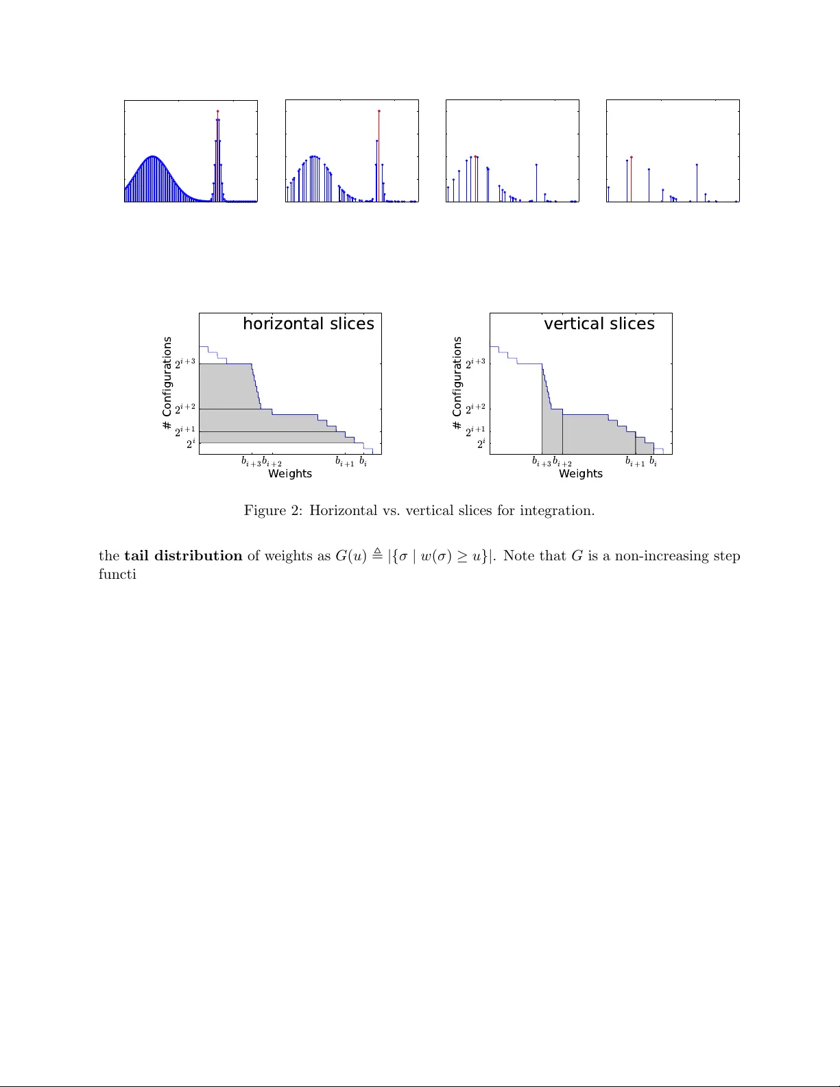
T aming the Curse of Dimensionalit y: Discrete In tegration b y Hashing and Optimization Stefano Ermon, Carla P . Gomes Dept. of Computer Science Cornell Univ ersity , Ithaca NY 14853, U.S.A. { ermonste,gomes } @cs.cornell.edu Ashish Sabharw al IBM W atson Researc h Center Y orkto wn Heights, NY 10598, U.S.A. ashish.sabharwal@us.ibm.com Bart Selman Dept. of Computer Science, Cornell Univ ersity , Ithaca NY 14853, U.S.A. selman@cs.cornell.edu F ebruary 15, 2013 Abstract In tegration is affected b y the curse of dimensionality and quickly b ecomes intractable as the dimensionalit y of the problem grows. W e propose a randomized algorithm that, with high probabilit y , giv es a constant-factor appro ximation of a general discrete integral defined o ver an exp onen tially large set. This algorithm relies on solving only a small n umber of instances of a discrete combinatorial optimization problem sub ject to randomly generated parity constrain ts used as a hash function. As an application, we demonstrate that with a small num b er of MAP queries we can efficien tly approximate the partition function of discrete graphical models, whic h can in turn b e used, for instance, for marginal computation or mo del selection. 1 In tro duction Computing in tegrals in v ery high dimensional spaces is a fundamen tal and largely unsolv ed problem of scien tific computation [4, 7, 24], with numerous applications ranging from m ac hine learning and statistics to biology and physics. As the volume grows exp onen tially in the dimensionality , the problem quickly b ecomes computationally intractable, a phenomenon traditionally kno wn as the curse of dimensionality [2]. W e revisit the problem of approximately computing discrete integrals, namely w eighted sums o ver (extremely large) sets of items. This problem encompasses sev eral imp ortan t probabilistic inference tasks, such as computing marginals or normalization constan ts (partition function) in graphical mo dels, which are in turn the cornerstones for parameter and structure learning [32]. Although we focus on the discrete case, the con tinuous case can in principle also b e addressed, as it can b e approximated by numerical integration. There are t wo common approac hes to appro ximate these large discrete sums: sampling and v ariational methods. V ariational metho ds [17, 32], often inspired by statistical ph ysics, are very fast but do not provide guarantees on the quality of the results. Since sampling and counting can be reduced to eac h other [16], approximate tec hniques 1 based on sampling are quite p opular, but they suffer from similar issues b ecause the n umber of samples required to obtain a statistically reliable estimate often grows exp onen tially in the problem size. Among sampling techniques, Marko v Chain Monte Carlo (MCMC) metho ds are asymptotically accurate, but guaran tees for practical applications exist only in a limited n umber of cases (fast mixing chains) [16, 18]. They are therefore often used in an heuristic manner. In practice, their p erformance crucially dep ends on the choice of the prop osal distributions, whic h often must be domain-specific and exp ert-designed [9, 21]. W e introduce a randomized scheme that computes with high probabilit y (1 − δ for any desired δ > 0) an appro ximately correct estimate (within a factor of 1 +  for an y desired  > 0) for general w eighted sums defined ov er exp onen tially large sets of items, suc h as the set of all possible v ariable assignments in a discrete probabilistic graphical model. F rom a computational complexit y p erspective, the coun ting problem w e consider is complete for the #P complexit y class [28], a set of problems encapsulating the en tire P olynomial Hierarch y and b eliev ed to b e significantly harder than NP . The k ey idea is to reduce this #P problem to a small n um b er (polynomial in the dimensionalit y) of instances of a (NP-hard) com binatorial optimization problem defined on the same space and sub ject to randomly generated “parit y” constrain ts. The rationale behind this approac h is that although com binatorial optimization is intractable in the worst case, it has witnessed great success in the past 50 years in fields such as Mixed Integer Programming (MIP) and propositional Satisfiabilit y T esting (SA T). Problems such as computing a Maxim um a Posteriori (MAP) assignment, although NP-hard, can in practice often be appro ximated [25] or solved exactly fairly efficiently [22, 23]. In fact, mo dern solvers can exploit structure in real-world problems and prune large p ortions of the searc h space, often dramatically reducing the runtime. In contrast, in a #P counting problem such as computing a marginal probabilit y , one needs to consider con tributions of an exponentially large n umber of items. Our algorithm, called W eighted- I n tegrals-And- S ums-By- H ashing ( WISH ), relies on randomized hashing techniques to “evenly cut” a high dimensional space. Suc h hashing was in tro duced b y V aliant and V azirani [29] to study the relationship b et w een the num b er of solutions and the hardness of a combinatorial search. These techniques were also applied by Gomes et al. [11, 12] to obtain b ounds on the num b er of solutions for the SA T problem. Our w ork is more general in that it can handle general w eighted sums, such as the ones arising in probabilistic inference for graphical mo dels. Our work is also closely related to recent w ork b y Hazan and Jaakkola [14], who obtain a low er b ound on the partition function b y taking suitable exp ectations of a com bination of MAP queries o ver randomly p erturbed mo dels. W e improv e up on this in tw o crucial asp ects, namely , our estimate is a constant factor appro ximation of the true partition function (while their b ounds ha ve no tigh tness guarantee), and we provide a concentration result showing that our b ounds hold not just in exp ectation but with high probability with a p olynomial n um b er of MAP queries. Note that this is consistent with known complexit y results regarding #P and BPP NP ; see Remark 1 b elo w. W e demonstrate the practical efficacy of the WISH algorithm in the con text of computing the partition function of random Clique-structured Ising models, Grid Ising mo dels with kno wn ground truth, and a challenging combinatorial application (Sudoku puzzle) completely out of reach of tec hniques such as Mean Field and Belief Propagation. W e also consider the Mo del Selection problem in graphical models, specifically in the context of hand-written digit recognition. W e show that our “anytime” and highly parallelizable algorithm can handle these problems at a level of accuracy and scale w ell b eyond the curren t state of the art. 2 2 Problem Statemen t and Assumptions Let Σ b e a (large) set of items. Let w : Σ → R + b e a non-negativ e function that assigns a w eight to each element of Σ. W e wish to (approximately) compute the total w eight of the set, defined as the following discrete in tegral or “partition function” W = X σ ∈ Σ w ( σ ) (1) W e as sume w is giv en as input and that it can b e compactly represen ted, for instance in a factored form as the pro duct of conditional probabilities tables. Note how ev er that our results are more general and do not rely on a factored representation. Assumption: W e assume to hav e access to an optimization or acle that can solve the following constrained optimization problem max σ ∈ Σ w ( σ )1 {C } ( σ ) (2) where 1 {C } : Σ → { 0 , 1 } is an indicator function for a compactly represen ted subset C ⊆ Σ, i.e., 1 {C } ( σ ) = 1 iff σ ∈ C . F or concreteness, we discuss our setup and assumptions in the con text probabilistic graphical mo dels, which is our motiv ating application. 2.1 Inference in Graphical Mo dels W e consider a graphical mo del sp ecified as a factor graph with N = | V | discrete random v ariables x i , i ∈ V where x i ∈ X i . The global random v ector x = { x s , s ∈ V } takes v alue in the cartesian pro duct X = X 1 × X 2 × · · · × X N . W e consider a probability distribution o ver x ∈ X (called configurations ) p ( x ) = 1 Z Q α ∈I ψ α ( { x } α ) that factors in to p otentials or factors ψ α : { x } α 7→ R + , where I is an index set and { x } α ⊆ V a subset of v ariables the factor ψ α dep ends on, and Z is a normalization constant kno wn as the partition function . Giv en a graphical mo del, w e let Σ = X b e the set of all p ossible configurations (v ariable assignmen ts). Define a w eight function w : X → R + that assigns to eac h configuration a score prop ortional to its probability: w ( x ) = Q α ∈I ψ α ( { x } α ). Z ma y then b e rewritten as Z = X x ∈X w ( x ) = X x ∈X Y α ∈I ψ α ( { x } α ) (3) Computing Z is typically intractable b ecause it inv olv es a sum o ver an exponential num b er of con- figurations, and is often the most challenging inference task for many families of graphical mo dels. Computing Z is how ever needed for man y inference and learning tasks, suc h as ev aluating the lik e- liho od of data for a giv en model, computing marginal probabilities, and parameter estimation [32]. In the con text of graphical models inference, we assume to ha ve access to an optimization oracle that can answer Maxim um a Posteriori (MAP) queries, namely , solve the following constrained optimization problem arg max x ∈X p ( x | C ) that is, we can find the most likely state (and its w eight) given some evidence C . This is a strong assumption b ecause MAP inference is kno wn to b e an NP-hard problem in general. Notice how ever that computing Z is a #P-complete problem, a complexity class believed to b e ev en harder than NP . 3 2.2 Quadratures of In tegrals Supp ose we are given a quadrature for a con tinuous (m ultidimensional) integral of a function f : R n → R + o ver a high dimensional set S ⊆ R n Z S f ( x )d x ≈ X x ∈X w ( x ) = W where X is some discretization of S (e.g., grid based), and w ( x ) approximates the in tegral of f ( x ) o ver the corresponding element of volume. In this case, we require a compact representation for w and access to an oracle able to optimize the discretized function, sub ject to arbitrary constraints. See, e.g., Figure 1. F or simplicit y , in the follo wing we will restrict ourselves to the binary case, i.e., Σ = X = { 0 , 1 } n . The general multinomial case where the sum is ov er X 1 × X 2 × · · · × X N can b e transformed into the former case using a binary representation, requiring d log 2 |X i |e bits (binary v ariables) p er dimension i . 3 Preliminaries W e review some results on the construction and prop erties of univ ersal hash functions; cf. [10, 27]. A reader already familiar with these results ma y skip to the next section. Definition 1. A family of functions H = { h : { 0 , 1 } n → { 0 , 1 } m } is pairwise indep endent if the follo wing t wo conditions hold when H ← R H is a function c hosen uniformly at random from H . 1) ∀ x ∈ { 0 , 1 } n , the random v ariable H ( x ) is uniformly distributed in { 0 , 1 } m . 2) ∀ x 1 , x 2 ∈ { 0 , 1 } n x 1 6 = x 2 , the random v ariables H ( x 1 ) and H ( x 2 ) are indep endent. A simple wa y to construct such a function is to think about the family H of all p ossible func- tions { 0 , 1 } n → { 0 , 1 } m . This is a family of not only pairwise independent but ful ly indep enden t functions. How ev er, each function requires m 2 n bits to b e represen ted, and is thus impractical in the t ypical case where n is large. On the other hand, p airwise indep endent hash functions can b e constructed and represented in a muc h more compact w ay as follows; see Appendix for a pro of. Prop osition 1. L et A ∈ { 0 , 1 } m × n , b ∈ { 0 , 1 } m . The family H = { h A,b ( x ) : { 0 , 1 } n → { 0 , 1 } m } wher e h A,b ( x ) = Ax + b mo d 2 is a family of p airwise indep endent hash functions. The space C = { x : h A,b ( x ) = p } has a nice geometric interpretation as the translated nullspace of the random matrix A . It is therefore a finite dimensional vector space, with op erations defined on the field F (2) (arithmetic mo dulo 2). W e will refer to constraints in the form Ax = b mo d 2 as parit y constrain ts , as they can be rewritten in terms of X ORs op erations as A i 1 x 1 ⊕ A i 2 x 2 ⊕ · · · ⊕ A in x n = b i . 4 The WISH Algorithm W e start with the in tuition b ehind our algorithm to approximate the v alue of W called W eighted- I n tegrals-And- S ums-By- H ashing ( WISH ). Computing W as defined in Equation (1) is challenging because the sum is defined ov er an exp onen tially large num b er of items, i.e., | Σ | = 2 n when there are n binary v ariables. Let us define 4 0 50 100 0 0.5 1 1.5 2 Items (configurations) Weight 0 50 100 0 0.5 1 1.5 2 Items (configurations) Weight 0 50 100 0 0.5 1 1.5 2 Items (configurations) Weight 0 50 100 0 0.5 1 1.5 2 Items (configurations) Weight Figure 1: Visualization of the “thinning” effect of random parit y constraints, after adding 0, 1, 2, and 3 parit y constraints. Leftmost plot sho ws the original function to in tegrate. Constrained optimal solution in red. b i + 3 b i + 2 b i + 1 b i W e i g h t s 2 i + 3 2 i + 2 2 i + 1 2 i # C o n f i g u r a t i o n s h o r i z o n t a l sl i c e s b i + 3 b i + 2 b i + 1 b i W e i g h t s 2 i + 3 2 i + 2 2 i + 1 2 i # C o n f i g u r a t i o n s v e r t i c a l sl i c e s Figure 2: Horizon tal vs. v ertical slices for integration. the tail distribution of w eights as G ( u ) , |{ σ | w ( σ ) ≥ u }| . Note that G is a non-increasing step function, changing v alues at no more than 2 n p oin ts. Then W may b e rewritten as R R + G ( u )d u , i.e., the total ar e a A under the G ( u ) vs. u curv e. One wa y to approximate W is to (implicitly) divide this area A in to either horizontal or vertic al slices (see Figure 4), appro ximate the area in eac h slice, and sum up. Supp ose w e had an efficient procedure to estimate G ( u ) giv en an y u . Then it is not hard to see that one could create enough slices b y dividing up the x-axis, estimate G ( u ) at these p oints, and estimate the area A using quadrature. How ev er, the natural wa y of doing this to an y degree of accuracy would require a num b er of slices that grows at least logarithmically with the w eight range on the x-axis, whic h is undesirable. Alternativ ely , one could split the y-axis, i.e., the G ( u ) v alue range [0 , 2 n ], at geometrically gro wing v alues 1 , 2 , 4 , · · · , 2 n , i.e., into bins of sizes 1 , 1 , 2 , 4 , · · · , 2 n − 1 . Let b 0 ≥ b 1 ≥ · · · ≥ b n b e the weigh ts of the configurations at the split p oints. In other words, b i is the 2 i -th quantile of the w eight distribution. Unfortunately , despite the monotonicit y of G ( u ), the area in the horizontal slice defined b y eac h bin is difficult to b ound, as b i and b i +1 could be arbitrarily far from eac h other. Ho wev er, the area in the vertic al slice defined by b i and b i +1 m ust b e b ounded b et ween 2 i ( b i − b i +1 ) and 2 i +1 ( b i − b i +1 ), i.e., within a factor of 2. Thus, summing ov er the lo wer bound for all such slices and the left-most slice, the total area A m ust b e within a factor of 2 of P n − 1 i =0 2 i ( b i − b i +1 ) + 2 n b n = b 0 + P n i =1 2 i − 1 b i . Of course, we don’t kno w b i . But if we could appro ximate eac h b i within a factor of p , we w ould get a 2 p -approximation to the area A , i.e., to W . WISH pro vides an efficien t wa y to realize this strategy , using a combination of randomized hash 5 Algorithm 1 WISH ( w : Σ → R + , n = log 2 | Σ | , δ, α ) T ← l ln(1 /δ ) α ln n m for i = 0 , · · · , n do for t = 1 , · · · , T do Sample hash function h i A,b : Σ → { 0 , 1 } i , i.e. sample uniformly A ∈ { 0 , 1 } i × n , b ∈ { 0 , 1 } i w t i ← max σ w ( σ ) sub ject to Aσ = b mo d 2 end for M i ← Median( w 1 i , · · · , w T i ) end for Return M 0 + P n − 1 i =0 M i +1 2 i functions and an optimization oracle to appro ximate the b i v alues with high probability . Note that this metho d allows us to compute the partition function W (or the area A ) b y estimating w eights b i at n + 1 carefully c hosen p oints, whic h is “only” an optimization problem. The key insight to compute the b i v alues is as follows. Supp ose we apply to configurations in Σ a randomly sampled pairwise indep enden t hash function with 2 m buc kets and use an optimization oracle to compute the w eight w m of a he aviest configuration in a fixed (arbitrary) buc ket. If we rep eat this process T times and consistently find that w m ≥ w ∗ , then we can infer b y the prop erties of hashing that at least 2 m configurations (globally) are lik ely to ha ve weigh t at least w ∗ . By the same token, if there w ere in fact at least 2 m + c configurations of a heavier w eight ˆ w > w ∗ for some c > 0, there is a go od chance that the optimization oracle will find w m ≥ ˆ w and w e w ould not underestimate the w eight of the 2 m -th heaviest configuration. As w e will see shortly , this pro cess, using pairwise indep enden t hash functions to k eep v ariance low, allows us to estimate b i accurately with only T = O(ln n ) samples. The pseudo co de of WISH is sho wn as Algorithm 1. It is parameterized by the w eight function w , the dimensionalit y n , a correctness parameter δ > 0, and a constant α > 0. Notice that the algorithm requires solving only Θ( n ln n ln 1 /δ ) optimization instances (MAP inference) to compute a sum defined ov er 2 n items. In the following section, w e formally pro ve that the output is a constan t factor approximation of W with probability at least 1 − δ (probability o ver the choice of hash functions). Figure 1 sho ws the working of the algorithm. As more and more random parit y constrain ts are added in the outer lo op of the algorithm (“lev els” increasing from 1 to n ), the configuration space is (pairwise-uniformly) thinned out and the optimization oracle selects the hea viest (in red) of the surviving configurations. The final output is a w eighted sum ov er the median of T such modes obtained at each lev el. Remark 1. The parity constraints Aσ = b mo d 2 do not change the worst-case complexity of an NP-hard optimization problem. Our result is thus consistent with the fact that #P can b e appro ximated in BPP NP , that is, one can approximately count the n umber of solutions with a randomized algorithm and a p olynomial n umber of queries to an NP oracle [10]. Remark 2. Although the parity constraints w e impose are simple linear equations ov er a field, they can mak e the optimization harder. F or instance, finding a configuration with the smallest Hamming weigh t satisfying a set of parit y constraints is known to b e NP-hard, i.e. equiv alen t to computing the minim um distance of a parit y co de [3, 30]. On the other hand, most lo w density parit y chec k co des can be solved extremely fast in practice using heuristic methods such as message 6 passing. Remark 3. Each of the optimization instances can b e solv ed indep endently , allowing natural massiv e parallelization . W e will also discuss how the algorithm can b e used in an an ytime fashion, and the implications of obtaining sub optimal solutions. 5 Analysis Since many configurations can hav e iden tical weigh t, it will help for the purp oses of the analysis to fix, w.l.o.g., a w eight-based ordering of the configurations, and a natural partition of the | Σ | = 2 n configurations into n + 1 bins that the ordering induces. Definition 2. Fix an ordering σ i , 1 ≤ i ≤ 2 n , of the configurations in Σ suc h that for 1 ≤ j < 2 n , w ( σ j ) ≥ w ( σ j +1 ). F or i ∈ { 0 , 1 , · · · , n } , define b i , w ( σ 2 i ). Define a sp ecial bin B , { σ 1 } and, for i ∈ { 0 , 1 , · · · , n − 1 } , define bin B i , { σ 2 i +1 , σ 2 i +2 , · · · , σ 2 i +1 } . Note that bin B i has precisely 2 i configurations. F urther, for all σ ∈ B i , it follo ws from the definition of the ordering that w ( σ ) ∈ [ b i +1 , b i ]. This allo ws us to b ound the sum of the weigh ts of configurations in B i (the “horizontal” slices) b et w een 2 i b i +1 and 2 i b i . 5.1 Estimating the T otal W eigh t Our main theorem is that Algorithm 1 provides a constant factor approximation to the partition function. Theorem 1. F or any δ > 0 and p ositive c onstant α ≤ 0 . 0042 , A lgorithm 1 makes Θ( n ln n ln 1 /δ ) MAP queries and, with pr ob ability at le ast (1 − δ ) , outputs a 16-appr oximation of W = P σ ∈ Σ w ( σ ) . The pro of relies on t wo in termediate results whose pro ofs ma y b e found in the App endix. Lemma 1. L et M i = Median( w 1 i , · · · , w T i ) b e define d as in Algorithm 1 and b i as in Definition 2. Then, for al l c ≥ 2 , ther e exists an α ∗ ( c ) > 0 such that for 0 < α ≤ α ∗ ( c ) , Pr  M i ∈ [ b min { i + c,n } , b max { i − c, 0 } ]  ≥ 1 − exp( − αT ) Lemma 2. L et L 0 , b 0 + P n − 1 i =0 b min { i + c +1 ,n } 2 i and U 0 , b 0 + P n − 1 i =0 b max { i +1 − c, 0 } 2 i . Then U 0 ≤ 2 2 c L 0 . Pr o of of The or em 1. It is clear from the pseudo code of Algorithm 1 that it makes Θ( n ln n ln 1 /δ ) MAP queries. F or accuracy analysis, w e can write W as: W , 2 n X j =1 w ( σ j ) = w ( σ 1 ) + n − 1 X i =0 X σ ∈ B i w ( σ ) ∈ " b 0 + n − 1 X i =0 b i +1 2 i , b 0 + n − 1 X i =0 b i 2 i # , [ L, U ] Note that U ≤ 2 L b ecause 2 L = 2 b 0 + P n − 1 i =0 b i +1 2 i +1 = 2 b 0 + P n ` =1 b ` 2 ` = b 0 + P n ` =0 b ` 2 ` ≥ U . Hence, if we had access to the true v alues of all b i , we could obtain a 2-approximation to W . 7 W e do not kno w true b i v alues, but Lemma 1 sho ws that the M i v alues computed b y Algorithm 1 are sufficien tly close to b i with high probabilit y . Recall that M i is the median of MAP v alues computed by adding i random parit y constrain ts and rep eating the pro cess T times. Sp ecifically , for c ≥ 2, it follows from Lemma 1 that for 0 < α ≤ α ∗ ( c ), Pr " n \ i =0  M i ∈ [ b min { i + c,n } , b max { i − c, 0 } ]  # ≥ 1 − n exp( − α T ) ≥ (1 − δ ) for T = log(1 /δ ) α log n , and M 0 = b 0 . Thus, with probabilit y at least (1 − δ ) the output of Algorithm 1, M 0 + P n − 1 i =0 M i +1 2 i , lies in the range: " b 0 + n − 1 X i =0 b min { i + c +1 ,n } 2 i , b 0 + n − 1 X i =0 b max { i +1 − c, 0 } 2 i # Let us denote this range [ L 0 , U 0 ]. By monotonicit y of b i , L 0 ≤ L ≤ U ≤ U 0 . Hence, W ∈ [ L 0 , U 0 ]. Applying Lemma 2, w e ha ve U 0 ≤ 2 2 c L 0 , which implies that with probabilit y at least 1 − δ the output of Algorithm 1 is a 2 2 c appro ximation of W . F or c = 2, observing that α ∗ (2) ≥ 0 . 0042 (see pro of of Lemma 1), w e obtain a 16-appro ximation for 0 < α ≤ 0 . 0042. 5.2 Estimating the T ail Distribution W e can also estimate the en tire tail distribution of the weigh ts, defined as G ( u ) , |{ σ | w ( σ ) ≥ u }| . Theorem 2. L et M i b e define d as in Algorithm 1, u ∈ R + , and q ( u ) b e the maximum i such that ∀ j ∈ { 0 , · · · , i } , M j ≥ u . Then, for any δ > 0 , with pr ob ability ≥ (1 − δ ) , 2 q ( u ) is an 8-appr oximation of G ( u ) c ompute d using O( n ln n ln 1 /δ ) MAP queries. While this is an interesting result in its o wn right, if the goal is to estimate the total w eight W , then the sc heme in Section 5.1, requiring a total of only Θ( n ln n ln 1 /δ ) MAP queries, is more efficien t than first estimating the tail distribution for several v alues of u . 5.3 Impro ving the Approximation F actor Giv en a κ -approximation algorithm such as Algorithm 1 and an y  > 0, w e can design a (1 +  )- appro ximation algorithm with the follo wing construction. Let ` = log 1+  κ . Define a new set of configurations Σ ` = Σ × Σ × · · · × Σ, and a new weigh t function w 0 : Σ ` → R as w 0 ( σ 1 , · · · , σ ` ) = w ( σ 1 ) w ( σ 2 ) · · · w ( σ ` ). Prop osition 2. L et c W b e a κ -appr oximation of P σ 0 ∈ Σ ` w 0 ( σ 0 ) . Then c W 1 /` is a κ 1 /` -appr oximation of P σ ∈ Σ w ( σ ) . T o see wh y this holds, observ e that W 0 = P σ 0 ∈ Σ ` w 0 ( σ 0 ) =  P σ ∈ Σ w ( σ )  ` = W ` . Since 1 κ W 0 ≤ c W ≤ κW 0 , we obtain that c W 1 /` m ust be a κ 1 /` = 1 +  approximation of W . Note that this construction requires running Algorithm 1 on an enlarged problem with ` times more v ariables. Although the n umber of optimization queries gro ws polynomially with ` , increasing the num b er of v ariables migh t significan tly increase the run time. 8 5.4 F urther Appro ximations When the instances defined in the inner loop are not solv ed to optimalit y , Algorithm 1 still pro vides appro ximate lower b ounds on W with high probabilit y . Theorem 3. L et e w t i b e sub optimal solutions for the optimization pr oblems in Algorithm 1, i.e., e w t i ≤ w t i . L et f W b e the output of Algorithm 1 with these sub optimal solutions. Then, for any δ > 0 , with pr ob ability at le ast 1 − δ , f W 16 ≤ W . F urther, if e w t i ≥ 1 L w t i for some L > 0 , then with pr ob ability at le ast 1 − δ , f W is a 16 L - appr oximation to W . The output is alw ays an approximate lo w er b ound, even if the optimization is stopped early . The lo wer b ound is monotonically non-decreasing ov er time, and is guaranteed to even tually reac h within a constant factor of W . W e th us hav e an an ytime algorithm. 6 Exp erimen tal Ev aluation W e implemen ted WISH using the open source solv er T oulBar2 [1] to solv e the MAP inference prob- lem. T oulBar2 is a complete solv er (i.e., given enough time, it will find an optimal solution and pro vide an optimality certificate), and it was one of the winning algorithms in the UAI-2010 infer- ence comp etition. W e augmen ted T oulBar2 with the IBM ILOG CPLEX CP Optimizer 12.3 based tec hniques b orrow ed from Gomes et al. [13] to efficiently handle the random parit y constraints. Sp ecifically , the set of equations Ax = b mo d 2 are linear equations ov er the field F (2) and thus allo w for efficien t propagation and domain filtering using Gaussian Elimination. F or our exp eriments, w e run WISH in parallel using a compute cluster with 642 cores. W e assign eac h optimization instance in the inner lo op to one core, and finally pro cess the results when all optimization instances hav e b een solved or ha ve reac hed a timeout. F or comparison, we consider T ree Rew eighted Belief Propagation [31] whic h provides an upper b ound on Z , Mean Field [32] which pro vides a lo wer b ound, and Loopy Belief Propagation [20] whic h pro vides an estimate with no guaran tees. W e use the implemen tations of these algorithms a v ailable in the LibD AI library [19]. 6.1 Pro v ably Accurate Approximations F or our first exp erimen t, w e consider the problem of computing the partition function, Z (cf. Eqn. (3)), of random Clique-structured Ising mo dels on n binary v ariables x i ∈ { 0 , 1 } for i ∈ { 1 , · · · , n } . The in teraction b et ween x i and x j is defined as ψ ij ( x i , x j ) = exp( − w ij ) when x i 6 = x j , and 1 otherwise, where w ij is uniformly sampled from [0 , w p | i − j | ] and w is a parameter set to 0 . 2. W e further in- ject some structure b y in tro ducing a closed c hain of strong repulsiv e in teractions uniformly sampled from [ − 10 w, 0]. W e consider models with n ranging from 10 to 60. These models hav e treewidth n and can b e solved exactly (by brute force) only up to ab out n = 25 v ariables. Figure 4(a) shows the results using v arious metho ds for v arying problem size. W e also computed ground truth for n ≤ 25 b y brute force en umeration. While other metho ds start to div erge from the ground truth at around n = 25, our estimate, as predicted by Theorem 1, remains v ery accurate, visually o verlapping in the plot. The actual estimation error is m uch smaller than the worst-case factor of 16 guaran teed by Theorem 1, as in practice o ver- and under-estimation errors tend to 9 cancel out. F or n > 25 w e don’t hav e ground truth, but other metho ds fall wel l outside the pro v able interv al provided b y WISH , rep orted as an error bar that is v ery small compared to the magnitude of errors made b y the other metho ds. All optimization instances generated b y WISH for n ≤ 60 w ere solved (in parallel) to optimality within a timeout of 8 hours, resulting in high confidence tigh t appro ximations of the partition function. W e are not aw are of an y other practical metho d that can provide suc h guarantees for coun ting problems of this size, i.e., a weigh ted sum defined o ver 2 60 items. 6.2 An ytime Usage with Sub optimal Solutions Next, we inv estigate the qualit y of our results when not all of the optimization instances can b e solv ed to optimality b ecause of timeouts, so that the strong theoretical guarantees of Theore m 1 do not apply (although Theorem 3 still applies). W e consider 10 × 10 binary Grid Ising models, for which ground truth can b e computed using the junction tree metho d [32]. W e use the same exp erimen tal setup as Hazan and Jaakk ola [14], who also use random MAP queries to derive b ounds (without a tightness guarantee) on the partition function. Sp ecifically , we ha ve n = 100 binary v ariables x i ∈ {− 1 , 1 } with in teraction ψ ij ( x i , x j ) = exp( w ij x i x j ). F or the attractive case, w e dra w w ij from [0 , w ]; for the mixed case, from [ − w , w ]. The “lo cal field” is ψ ij ( x i ) = exp( f i x i ) where f i , the strength at site i , is sampled uniformly from [ − f , f ], where f is a parameter with v alue 0.1 or 1.0. Figure 3 reports the estimation err or for the log-partition function, when using a timeout of 15 min utes. W e see that WISH pro vides accurate estimates for a wide range of w eights, often impro ving o ver all other methods. The sligh t p erformance drop of WISH for coupling strengths w ≈ 1 appears to occur b ecause in that w eigh t range the terms corresp onding to i ≈ n/ 2 parity constraints are the most s ignifican t in the output sum M 0 + P n − 1 i =0 M i +1 2 i . Empirically , optimization instances with roughly n/ 2 parit y constraints are often the hardest to solv e, resulting in p ossibly a significant underestimation of the v alue of W = Z when a timeout o ccurs. W e do not directly compare with the w ork of Hazan and Jaakk ola [14] as w e did not ha ve access to their co de. How ev er, a visual lo ok at their plots suggests that WISH would provide an impro vemen t in accuracy , although with longer runtime. 6.3 Hard Combinatorial Structures An in teresting and combinatorially challenging graphical mo del arises from Sudoku, which is a p opular num b er-placemen t puzzle where the goal is to fill a 9 × 9 grid (see Figure 4(b)) with digits from { 1 , · · · , 9 } so that the entries in each row, column, and 3 × 3 blo ck comp osing the grid, are all distinct. The puzzle can b e enco ded as a graphical mo del with 81 discrete v ariables with domain { 1 , · · · , 9 } , with p otentials ψ α ( { x } α ) = 1 if and only if all v ariables in { x } α are different, and α ∈ I where I is an index set containing the subsets of v ariables in each row, column, and blo c k. This defines a uniform probability distribution ov er all v alid complete Sudoku grids (a non-v alid grid has probability zero), and the normalization constant Z s equals the total num b er of v alid grids. It is kno wn that Z s = 6 . 671 × 10 21 . This n umber w as computed exactly with a combination of computer enumeration and clever exploitation of prop erties of the symmetry group [8]. Here, w e attempt to approximately compute this num b er using the general-purp ose scheme WISH . First, following F elgenhauer and Jarvis [8], w e simplify the problem by fixing the first blo ck as in Figure 4(b), obtaining a new problem o ver 72 v ariables whose normalization constant is 10 0 0.5 1 1.5 2 2.5 3 −40 −30 −20 −10 0 10 20 Coupling Strength Log partition function estimation error WISH Belief Propagation TRW−BP MeanField (a) Attractiv e. Field 0 . 1. 0 0.5 1 1.5 2 2.5 3 −30 −20 −10 0 10 20 Coupling Strength Log partition function estimation error WISH Belief Propagation TRW−BP MeanField (b) Attractiv e. Field 1 . 0. 0 0.5 1 1.5 2 2.5 3 −20 −10 0 10 20 30 40 50 60 Coupling Strength Log partition function estimation error WISH Belief Propagation TRW−BP MeanField (c) Mixed. Field 0 . 1. 0 0.5 1 1.5 2 2.5 3 −20 −10 0 10 20 30 40 50 Coupling Strength Log partition function estimation error WISH Belief Propagation TRW−BP MeanField (d) Mixed. Field 1 . 0. Figure 3: Estimation errors for the log-partition function on 10 × 10 randomly generated Ising Grids. Z 0 = Z s / 9! ≈ 2 54 . Next, since w e are dealing with a feasibility rather than optimization problem, w e replace T oulBar2 with CryptoMiniSA T [26], a SA T solv er des igned for un weigh ted cryptographic problems and whic h nativ ely supp orts parit y constraints. W e observ ed that WISH can consisten tly find solutions (60% of the times) after adding 52 random parit y constrain ts, while for 53 constrain ts the success rate drops below 0 . 5, at 45%. Therefore M i = 1 in Algorithm 1 for i ≤ 52 and there should th us b e at least 2 52 · 9! ≈ 1 . 634 × 10 21 solutions to the Sudoku puzzle. Although Theorem 1 cannot b e applied due to timeouts for larger v alues of i , this estimate is clearly v ery close to the known true coun t. In contrast, the simple “lo cal reasoning” done by v ariational metho ds is not p o werful enough to find even a single solution. Mean Field and Belief Propagation rep ort an estimated solution count of exp( − 237 . 921) and exp( − 119 . 307), resp., on a relaxed problem where violating a constraint giv es a p enalt y exp( − 10). 6.4 Mo del Selection Man y inference and learning tasks require computing the normalization constan t of graphical mod- els. F or instance, it is needed to ev aluate the likelihoo d of observed data for a given mo del. This is necessary for Mo del Selection, i.e., to rank candidate mo dels, or to trigger early stopping during training when the lik eliho o d of a v alidation set starts to decrease, in order to av oid ov erfitting [6]. 11 0 10 20 30 40 50 60 70 −350 −300 −250 −200 −150 −100 −50 0 50 Size Log partition function estimate WISH Belief Propagation TRW−BP MeanField Ground Truth (a) Log parition function for cliques. 1 2 3 4 5 6 7 8 9 (b) Sudoku puzzle. (c) Confabulations from RBM models. Figure 4: Clique Ising models, hard combinatorial structure of Sudoku, and Mo del Selection for hand-written digits. 12 W e train Restricted Boltzmann Machines (RBM) [15] using Con trastiv e Div ergence (CD) [5, 33] on MNIST hand-written digits dataset. In an RBM there is a lay er of n h hidden binary v ariables h = h 1 , · · · , h n h and a lay er of n v binary visible units v = v 1 , · · · , v n v . The joint probabilit y distribution is given by P ( h, v ) = 1 Z exp( b 0 v + c 0 h + h 0 W v ). W e use n h = 50 hidden units and n v = 196 visible units. W e learn the parameters b, c, W using CD- k for k ∈ { 1 , 10 , 15 } , where k denotes the n umber of Gibbs sampling steps used in the inference phase, with 15 training ep o c hs and minibatches of size 20. Figure 4(c) depicts confabulations (samples generated with Gibbs sampling) from the three learned models. T o ev aluate the loglikelihoo d of the data and determine whic h mo del is the b est, one needs to compute Z . W e use WISH to estimate this quan tity , with a timeout of 10 minutes, and then rank the mo dels according to the a v erage loglikelihoo d of the data. The scores w e obtain are − 41 . 70 , − 40 . 35 , − 40 . 01 for k = 1 , 10 , 15, resp ectiv ely (larger scores means higher likelihoo d). In this case T oulBar2 w as not able to prov e optimality for all instances, so only Theorem 3 applies to these results. Although we do not ha ve ground truth, it can b e seen that the ranking of the mo dels is consistent with what visually app ears closer to a large collection of hand-written digits in Figure 4(c). Note that k = 1 is clearly not a go o d representativ e, because of the highly unev en distribution of digit o ccurrences. The ranking of WISH is also consisten t with the fact that using more Gibbs sampling steps in the inference phase should provide b etter gradien t estimates and therefore a b etter learned mo del. In con trast, Mean Field results in scores − 35 . 47 , − 36 . 08 , − 36 . 84, resp., and w ould thus rank the mo dels in reverse order of what is visually the most representativ e order. 7 Conclusion W e in tro duced WISH , a randomized algorithm that, with high probability , giv es a constan t-factor appro ximation of a general discrete in tegral defined o ver an exp onen tially large set. WISH reduces the in tractable coun ting problem to a small num b er of instances of a combinatorial optimization problem sub ject to parit y constraints used as a hash function. In the context of graphical mo dels, w e sho w ed ho w to appro ximately compute the normalization constan t, or partition function, using a small num b er of MAP queries. Using state-of-the-art combinatorial optimization to ols, we are th us able to provide discrete integral or partition function estimates with approximation guarantees at a scale that could till now b e handled only heuristically . Finally , our metho d is a massively parallelizable and anytime algorithm which can also b e stopp ed early to obtain empirically accurate estimates that provide lo wer b ounds with a high probability . Ac kno wledgmen ts Supp orted by NSF Exp editions in Computing grant on Computational Sustainability #0832782 and NSF Computing Researc h Infrastructure gran t #1059284. References [1] D. Allouc he, S. de Givry , and T. Sc hiex. T oulbar2, an op en source exact cost function netw ork solv er. T echnical rep ort, INRIA, 2010. 13 [2] R. Bellman. A daptive c ontr ol pr o c esses: A guide d tour . Princeton Univ ersity Press (Princeton, NJ), 1961. [3] E. Berlek amp, R. McEliece, and H. V an Tilb org. On the inheren t intractabilit y of certain co ding problems. Information The ory, IEEE T r ansactions on , 24(3):384–386, 1978. [4] J. Cai and X. Chen. A decidable dic hotomy theorem on directed graph homomorphisms with non- negativ e w eights. In FOCS , 2010. [5] M. Carreira-P erpinan and G. Hin ton. On contrastiv e divergence learning. In Artificial Intel ligenc e and Statistics , vol. 2005, page 17, 2005. [6] G. Desjardins, A. Courville, and Y. Bengio. On trac king the partition function. In A dvanc es in Neur al Information Pr o c essing Systems 24 , pp. 2501–2509, 2011. [7] M. Dyer, A. F rieze, and R. Kannan. A random p olynomial-time algorithm for approximating the v olume of conv ex bo dies. JACM , 38(1):1–17, 1991. [8] B. F elgenhauer and F. Jarvis. Enumerating p ossible sudoku grids. Mathematic al Sp e ctrum , 2005. [9] M. Girolami and B. Calderhead. Riemann manifold langevin and hamiltonian monte carlo metho ds. Journal of the R oyal Statistic al So ciety , 73(2):123–214, 2011. [10] O. Goldreich. Randomized metho ds in computation. L e ctur e Notes , 2011. [11] C. Gomes, A. Sabharwal, and B. Selman. Model coun ting: A new strategy for obtaining goo d b ounds. In AAAI , pp. 54–61, 2006. [12] C. Gomes, A. Sabharwal, and B. Selman. Near-uniform sampling of com binatorial spaces using X OR constrain ts. A dvanc es In Neur al Information Pr o c essing Systems , 19:481–488, 2006. [13] C. P . Gomes, W. J. v an Hoeve, A. Sabharw al, and B. Selman. Counting CSP solutions using generalized X OR constrain ts. In AAAI , 2007. [14] T. Hazan and T. Jaakk ola. On the partition function and random maximum a-posteriori p erturbations. In ICML , 2012. [15] G. Hinton, S. Osindero, and Y. T eh. A fast learning algorithm for deep b elief nets. Neur al c omputation , 18(7):1527–1554, 2006. [16] M. Jerrum and A. Sinclair. The Marko v chain Monte Carlo metho d: an approach to approximate coun ting and integration. Appr oximation algorithms for NP-har d pr oblems , pp. 482–520, 1997. [17] M. Jordan, Z. Ghahramani, T. Jaakk ola, and L. Saul. An introduction to v ariational metho ds for graphical mo dels. Machine le arning , 37(2):183–233, 1999. [18] N. Madras. L e ctur es on Monte Carlo Metho ds . American Mathematical So ciet y , 2002. ISBN 0821829785. [19] J. Mo oij. libDAI: A free and open source c++ library for discrete approximate inference in graphical mo dels. JMLR , 11:2169–2173, 2010. [20] K. Murph y , Y. W eiss, and M. Jordan. Lo op y belief propagation for approximate inference: An empirical study . In UAI , 1999. [21] I. Murra y and Z. Ghahramani. Bay esian learning in undirected graphical mo dels: approximate mcmc algorithms. In UAI , 2004. 14 [22] J. Park. Using weigh ted max-sat engines to solve mp e. In AAAI-2002 , pp. 682–687, 2002. [23] J. D. P ark. MAP complexity results and approximation methods. In UAI , 2002. [24] M. Simonovits. Ho w to compute the v olume in high dimension? Mathematic al pr o gr amming , 97(1): 337–374, 2003. [25] D. Sontag, T. Meltzer, A. Globerson, T. Jaakkola, and Y. W eiss. Tightening lp relaxations for map using message passing. In UAI , pp. 503–510, 2008. [26] M. So os, K. Nohl, and C. Castelluccia. Extending sat solv ers to cryptographic problems. SA T , 2009. [27] S. V adhan. Pseudorandomness. F oundations and T r ends in The or etic al Computer Scienc e , 2011. [28] L. V alian t. The complexit y of enumeration and reliabilit y problems. SIAM Journal on Computing , 8 (3):410–421, 1979. [29] L. V aliant and V. V azirani. NP is as easy as detecting unique solutions. The or etic al Computer Scienc e , 47:85–93, 1986. [30] A. V ardy . Algorithmic complexity in co ding theory and the minim um distance problem. In STOC , 1997. [31] M. W ain wrigh t. T ree-reweigh ted b elief propagation algorithms and appro ximate ML estimation via pseudo-momen t matc hing. In AIST A TS , 2003. [32] M. W ain wright and M. Jordan. Graphical mo dels, exp onen tial families, and v ariational inference. F oundations and T r ends in Machine L e arning , 1(1-2):1–305, 2008. [33] M. W elling and G. Hinton. A new learning algorithm for mean field b oltzmann mac hines. Artificial Neur al NetworksICANN 2002 , pp. 82–82, 2002. A App endix: Pro ofs Pr o of of Pr op osition 1. Immediately follows from Lemma 3. Lemma 3 (pairwise indep enden t hash functions construction) . L et a ∈ { 0 , 1 } n , b ∈ { 0 , 1 } . Then the family H = { h a,b ( x ) : { 0 , 1 } n → { 0 , 1 }} wher e h a,b ( x ) = a · x + b mo d 2 is a family of p airwise indep endent hash functions. The function h a,b ( x ) c an b e alternatively r ewritten in terms of X ORs op er ations ⊕ , i.e. h a,b ( x ) = a 1 x 1 ⊕ a 2 x 2 ⊕ · · · ⊕ a n x n ⊕ b . Pr o of. Uniformity is clear b ecause it is the sum of uniform Bernoulli random v ariables ov er the field F (2) (arithmetic mo dulo 2). F or pairwise indep endence, giv en an y tw o configurations x 1 , x 2 ∈ { 0 , 1 } n , consider the sets of indexes S 1 = { i : x 1 ( i ) = 1 } , S 2 = { i : x 2 ( i ) = 1 } . Then H ( x 1 ) = X i ∈ S 1 ∩ S 2 a i ⊕ X i ∈ S 1 \ S 2 a i ⊕ b = R ( S 1 ∩ S 2 ) ⊕ R ( S 1 \ S 2 ) ⊕ b H ( x 2 ) = R ( S 1 ∩ S 2 ) ⊕ R ( S 2 \ S 1 ) ⊕ b Note that R ( S 1 ∩ S 2 ), R ( S 1 \ S 2 ), R ( S 2 \ S 1 ) and b are indep endent as they dep end on disjoin t subsets of indep enden t v ariables. When x 1 6 = x 2 , this implies that ( H ( x 1 ) , H ( x 2 )) takes each v alue in { 0 , 1 } 2 with probability 1 / 4. 15 As pairwise independent random v ariables are fundamen tal to ols for derandomization of algo- rithms, more complicated constructions based larger finite fields generated b y a prime p o w er F ( q k ) where q is a prime n umber are known [27]. These constructions require a smaller n umber of ran- dom bits as input, and w ould therefore reduce the v ariance of our algorithm (which is deterministic except for the randomized hash function use). Pr o of of L emma 1. The cases where i + c > n or i − c < 0 are ob vious. F or the other cases, let’s define the set of the 2 j hea viest configurations as in Definition 2: X j = { σ 1 , σ 2 , · · · , σ 2 j } Define the following random v ariable S j ( h i A,b ) , X σ ∈X j 1 { Aσ = b mo d 2 } whic h giv es the num b er of elements of X j satisfying i random parit y constraints. The randomness is ov er the c hoice of A and b , whic h are uniformly sampled in { 0 , 1 } i × n and { 0 , 1 } i resp ectiv ely . By Prop osition 1, h i A,b : Σ → { 0 , 1 } i is sampled from a family of pairwise indep enden t hash functions. Therefore, from the uniformit y prop ert y in Definition 1, for any σ the random v ariable 1 { Aσ = b mo d 2 } is Bernoulli with probabilit y 1 / 2 i . By linearit y of exp ectation, E [ S j ( h i A,b )] = |X j | 2 i = 2 j 2 i F urther, from the pairwise indep endence prop ert y in Definition 1, V ar [ S j ( h i A,b )] = X σ ∈X j V ar  1 { Aσ = b mo d 2 }  = 2 j 2 i  1 − 1 2 i  Applying Chebyc hev Inequality , w e get that for any k > 0, Pr "     S j ( h i A,b ) − 2 j 2 i     > k s 2 j 2 i  1 − 1 2 i  # ≤ 1 k 2 Recall the definition of the random v ariable w i = max σ w ( σ ) sub ject to Aσ = b mo d 2 (the randomness is ov er the c hoice of A and b ). Then Pr[ w i ≥ b j ] = Pr[ w i ≥ w ( σ 2 j )] ≥ Pr[ S j ( h i A,b ) ≥ 1] whic h is the probability that at least one configuration from X j “surviv es” after adding i parity constrain ts. T o ensure that the probabilit y b ound 1 /k 2 pro vided b y Chebyc hev Inequality is smaller than a 1 / 2, w e need k > √ 2. W e use k = 3 / 2 for the rest of this proof, exploiting the following simple observ ations whic h hold for k = 3 / 2 and any c ≥ 2: k √ 2 c ≤ 2 c − 1 k √ 2 − c ≤ 1 − 2 − c 16 F or j = i + c and k and c as ab o ve, w e hav e that Pr[ w i ≥ b i + c ] ≥ Pr[ S i + c ( h i A,b ) ≥ 1] ≥ Pr  | S i + c ( h i ) − 2 c | ≤ 2 c − 1  ≥ Pr h | S i + c ( h i ) − 2 c | ≤ k √ 2 c i ≥ Pr "   S i + c ( h i A,b ) − 2 c   ≤ k s 2 c  1 − 1 2 i  # ≥ 1 − 1 k 2 = 5 / 9 > 1 / 2 Similarly , for j = i − c and k and c as ab ov e, w e ha ve Pr[ w i ≤ b i − c ] ≥ 5 / 9 > 1 / 2. Finally , using Chernoff inequalit y (since w 1 i , · · · , w T i are i.i.d. realizations of w i ) Pr [ M i ≤ b i − c ] ≥ 1 − exp( − α 0 ( c ) T ) (4) Pr [ M i ≥ b i + c ] ≥ 1 − exp( − α 0 ( c ) T ) (5) where α 0 (2) = 2(5 / 9 − 1 / 2) 2 , which giv es the desired result Pr [ b i + c ≤ M i ≤ b i − c ] ≥ 1 − 2 exp( α 0 ( c ) T ) = 1 − exp( − α ∗ ( c ) T ) where α ∗ (2) = ln 2 α 0 (2) = 2(5 / 9 − 1 / 2) 2 ln 2 > 0 . 0042 Pr o of of L emma 2. Observe that w e may rewrite L 0 as follows: L 0 = b 0 + n − 1 X i = n − c − 1 b n 2 i + n − c − 2 X i =0 b i + c +1 2 i = b 0 + n − 1 X i = n − c − 1 b n 2 i + n − 1 X j = c +1 b j 2 j − c − 1 17 Similarly , U 0 = b 0 + c − 1 X i =0 b 0 2 i + n − 1 X i = c b i +1 − c 2 i = b 0 + c − 1 X i =0 b 0 2 i + n − c X j =1 b j 2 j + c − 1 = 2 c b 0 + 2 c n − c X j =1 b j 2 j − 1 = 2 c b 0 + 2 c   c X j =1 b j 2 j − 1 + n − c X j = c +1 b j 2 j − 1   ≤ 2 c b 0 + 2 c   c X j =1 b 0 2 j − 1 + n − c X j = c +1 b j 2 j − 1   = 2 2 c b 0 + 2 2 c n − c X j = c +1 b j 2 j − 1 − c ≤ 2 2 c   b 0 + n − 1 X i = n − c − 1 b n 2 i + n − 1 X j = c +1 b j 2 j − c − 1   = 2 2 c L 0 This finishes the proof. Pr o of of The or em 2. As in the proof of Lemma 1, define the random v ariable S u ( h i A,b ) , X σ ∈{ σ | w ( σ ) ≥ u } 1 { Aσ = b mo d 2 } that gives the n umber of configurations with w eigh t at least u satisfying i random parit y constraints. Then for i ≤ b log G ( u ) c − c ≤ log G ( u ) − c using Cheb ychev and Chernoff inequalities as in Lemma 1 Pr [ M i ≥ u ] ≥ 1 − exp( − α 0 T ) F or i ≥ d log G ( u ) e + c ≥ log G ( u ) + c , using Cheb ychev and Chernoff inequalities as in Lemma 1 Pr[ M i < u ] ≥ 1 − exp( − α 0 T ) Therefore, Pr  1 2 c +1 2 q ( u ) ≤ G ( u ) ≤ 2 c +1 2 q ( u )  ≥ Pr   b log 2 G ( u ) c− c \ i =0 ( M i ≥ u ) \  M d log 2 G ( u ) e + c < u    ≥ 1 − n exp( − α 0 T ) ≥ 1 − δ This finishes the proof. 18 Pr o of of The or em 3. If e w t i ≤ w t i , from Theorem 1 with probability at least 1 − δ w e hav e f W ≤ M 0 + P n − 1 i =0 M i +1 2 i ≤ U B 0 . Since U B 0 2 2 c ≤ LB 0 ≤ W ≤ U B 0 , it follo ws that with probability at least 1 − δ , f W 2 2 c ≤ W . If w t i ≥ e w t i ≥ 1 L w t i , then from Theorem 1 with probability at least 1 − δ the output is 1 L LB 0 ≤ f W ≤ U B 0 , and LB 0 ≤ W ≤ U B 0 . 19