Combining Multiple Time Series Models Through A Robust Weighted Mechanism

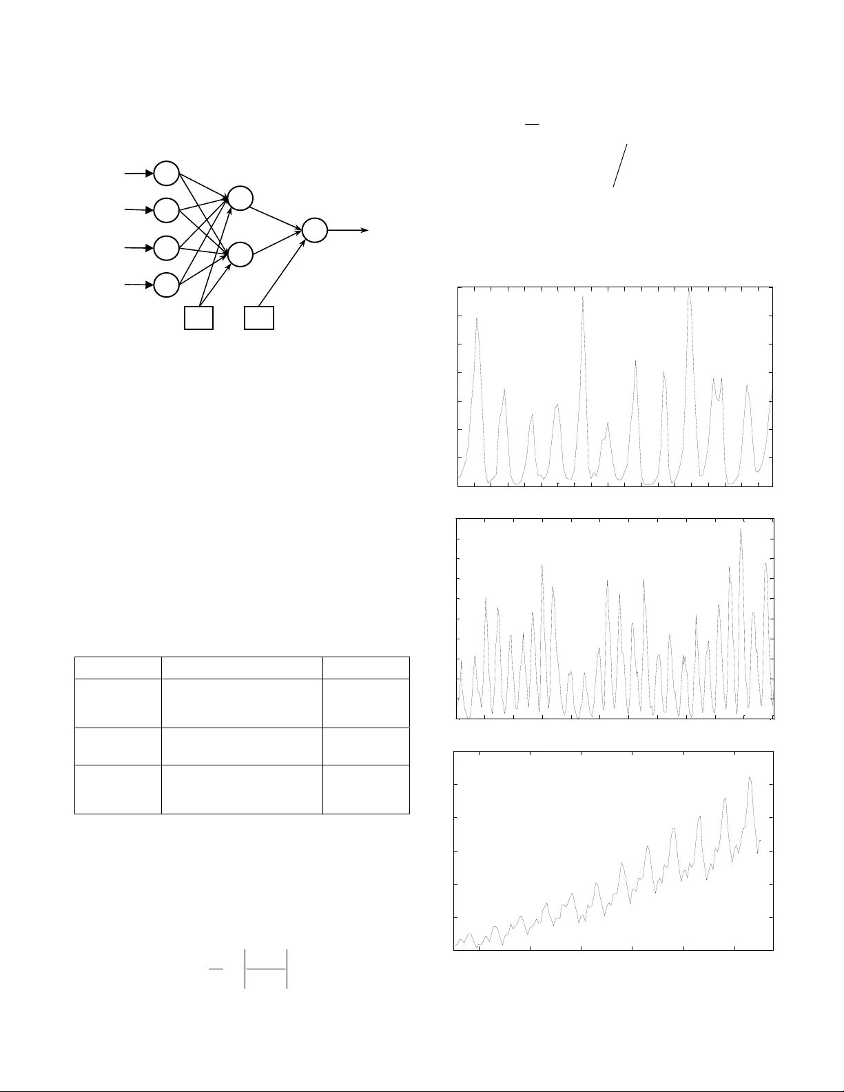
Combining Multiple Time Series Models Through A Robust Weighted Mechanism Ratnadip Adhikari School of Com puter and Sy stems Sciences Jawaharlal Nehr u University New Delhi, India Email: adhikari.ratan@gmail.co m R. K. Agrawal School of Com puter and Sy stems Sciences Jawaharlal Nehr u University New Delhi, India Email: rkajnu@gmail.com Abstract —Improvement of time series for ecasting accuracy through combining multiple models is an important as well as a dynamic area of research. As a re sult, various forecasts combination methods have b een developed in literat ure. However, most of them are based on simple linear ensemb le strategies and hence ignore th e possible re lationships between two or more participating models . In this paper, we propose a robust weighted nonlinear ensemble technique which considers the individual forecasts from different models as well as the correlations among th em while combining. Th e proposed ensemble is constructed using three well-know n forecasting models and is tested for three real-world time series. A comparison is made among th e proposed scheme and three other widely us ed linear combination meth ods, in terms of the obtained forecast errors. This comparison shows that our ensemble scheme p rovides significan tly lower fore cast errors than each individu al model as well as each of the four linear combination methods. Keywords-time series; forecast s combination; Box-Jenkins models; artificial neural netw or ks; support vector machines I. I NTRODUCTION Time series forecasting is a continuously growing research area with fundamenta l importa nce in many domains of business, finance, demography, science and e ngineering, etc. Improvement of forecasting accuracies has received extensive attentions from res earchers during the past two decades [1, 2]. In literature, it has been frequently observed that a suitable combina tion of multiple forecasts su bstantially improves the overall accuracy as well as outperforms each individual m odel [3, 4]. Combination st rategies are the best intuitive alternativ es to use, when there is a considerab le amount of unc ertainty associated wi th the selection of the optimal forecasting m odel. Mo reover, combining multiple forecasts reduces the errors ar ising from faulty assum ptions, bias, or mistakes in the data to a great extent. Starting with the benchm ark work of Bates and Grange r in 1969 [5], a number of fo recasts combination techniques have been developed in literature [6–8]. T he most popular among them are the weighted linear com binations, where the weights assigned to the individual m odels are either equal or decided according to some rigorous mathematical rule. Some common linear forecasts combination methods are the simple average, trimmed av erage, Winsorized average, median, error-based method, outperformance method, vari ance-based pooling, etc. [9, 10] . Although linear com bination techniques are easy to understand a nd implement , but they completely ignore the possible rel ationships among the parti cipating models in the ensemble. This l imitation has a neg ative effect on the forecasting accuracy of th e ensem ble, especially when the constituent forecasts are significantly correlated. Nonlinear forecast combinat ion is an area in wh ich the existing literatu re is quite limited and so has a strong need of furthe r develop ments [10]. In this paper, we propose a weighted nonlinear mechanism fo r combining forecasts from multiple tim e series models. Our proposed technique is partially motivated by the work of Freitas and Rodri gues [11] and it considers individual forecasts as well as correlations between pairs of forecasts for combining. Three forecasting models, viz. Autoregressive Integrated Moving Aver age (ARIMA), Artifici al Neural Network (ANN) and Support Vector Machine (SVM) are used to build up t he proposed ensemble. The ap propriate co mbination weig hts are determined from the performances of the individual models on the validation dataset s. The effectiveness of our proposed technique is empi rically tested on three real-world time series, in terms of three co mmon error measures: the Mean Absolute Percentage Error (MAPE), the Mean Squared Error (MSE), and the Average Relative Variance (ARV). Also, the forecasting performances of the proposed ensemble scheme for all three datasets are compared with three popular l inear combination methods. These are the simple average, the median and a weighted linear combination in which the weights are determined from the validatio n MAPE values, obtained by the individual forecast ing models. The rest of the paper is organized as follows. Secti on II presents some well-known lin ear forecasts combination techniques. Our nonl inear ensemble schem e is described in Section III. In Section IV, we discuss abou t the three time series forecasting models, which are used here to build up the proposed ensem ble. Experimental results are reported in Section V and in Section V I, we conclude this paper. II. L INEAR F ORCASTS C OMBINATION T ECHNIQUES In a linear combination tec hnique, the com bined forecast for the associated time series is calculated through a linear function of the individual fo recasts from the contributing models. Let, Y =[ y 1 , y 2 , …, y N ] T be the actual time series, which is to be forecasted using n different m odels and T () () () () 12 ˆ ˆˆ ˆ ,, , ii i i N yy y   =   Y … be its forecast obtained from the i th model ( i =1, 2,…, n ). Then, a linear com bination of these n forecasted series of the orig inal time series produces T () () () () 12 ˆ ˆˆ ˆ ,, , cc c c N yy y  =  Y … , given by: () () ( 1 ) ( 2 ) ( ) ˆˆ ˆ ˆ ,, , 1 , 2 , , . cn kk k k yf y y y k N =∀ = …… where, f is some linear function of the individual forecasts () ˆ i k y ( i =1, 2,…, n ; k =1, 2,…, N ). Thus, we have: () ( 1 ) ( 2 ) ( ) ( ) 12 1 ˆˆ ˆ ˆ ˆ . 1, 2 , , . n cn i ni kk k k k i yw y w y w y w y kN =   =+ + + =   ∀=  ∑ … … (1) Here, w i is the weight assigned to th e i th forecasting me thod. To ensure unbiasedness, it is often assumed that the wei ghts add up to unity. Some widely u sed linear combination techniques are briefly described below: • In the simple average , all models are assigned equal weights, i.e. w i =1 ⁄ n ( i =1, 2,…, n ) [9, 10]. • In the trimmed aver age , individual forecasts are combined by a simple ar ithmetic mean , excluding the worst performi ng k % of the models. A trimm ing of 10%–30% is usually recommended [9 , 10]. • In the Winsorized average , the i sm allest and i largest forecasts are select ed and respectively set as the ( i +1) th smallest and ( i +1) th largest forecasts [9]. • In the median-based com bining, the combination function f is the median of the individual forecasts. Median is sometimes preferred over simple average as it is less sensitive to extre me values [12, 13]. • In the error-based combining, the weight to each model is assigned to be the inverse of t he past forecast error (e.g. MSE, MAE, MAPE, etc.) of the corresponding model [3, 10]. • In the variance-based method, t he optimal weights are determined thro ugh the minimizat ion of the to tal Sum of Squared Erro r (SSE) [7, 10]. III. T HE P ROPOSED E NSEMBLE T ECHNIQUE As mentioned earl ier, a major disadvant age of a linear combination tech nique is that it co nsiders only the contributions o f the individual models, but total ly overlooks the possible relationships among them. As a result, there is a considerable reduction in the forecasting accuracy of a linear combination schem e, when two or more part icipating models in the ensemble are correlated. To overcome this limita tion, our ensemble techni que is developed as an extension of the usual linear combinatio n in order to deal with the p ossible correlations between pairs of forecasts. A. Mathematical Description Here we describe o ur ensemble method for combining three forecasts, but it can be easily generalized. Let, the actual test dataset o f a time series be Y =[ y 1 , y 2 , …, y N ] T with T () () () () 12 ˆ ˆˆ ˆ ,, , ii i i N yy y  =  Y … being its fore cast obtained from the i th method ( i =1, 2, 3). Let, µ ( i ) and σ ( i ) be the mean and standard deviation of () ˆ , i Y respectively. Then the combined forecast of Y is defined as: () () () () ( ) () () T () () () () 12 (1) ( 2 ) ( 3 ) 01 2 3 ( 1 )( 2 ) ( 2 )( 3 ) ( 3 )( 1 ) 12 3 2 ˆ ˆˆ ˆ ,, , , ˆˆ ˆ ˆ ˆˆ ˆ ˆ ˆ ˆ . ˆˆ 1, 2 , 3; 1, 2 , , cc c c N c kk k k kk k k k k ii ii kk yy y yw w y w y w y vv v v v v vy ik N θθ θ µσ   =    =+ + +   ++ +    =−   ==  Y … … (2) In (2), the nonlinear terms in calculating ( ) ˆ c k y are included to take into account the correlat ion effects between pairs of forecasts. The optimal weights are to be determined by minimizing the forecast SSE, given by: () ( ) 2 1 ˆ SSE N c k k k yy = =− ∑ (3) Now, for optim ization of the com bination weights, we ha ve: ( ) ( ) () () () SSE 0 SSE 0 . 0 , 1, 2 , 3 ; 1, 2 , 3 i j w ij θ  ∂∂ =   ∂∂ =   ==   (4) After computations of the associ ated partial derivatives in (4) and subsequent m athematical sim plifications, we can get the following system of linear equatio ns: T . +=    +=   Vw Z θ b Zw U θ d (5) where, [] [ ] ( ) () () ( ) ( ) ( ) ( ) () () ( ) ( ) ( ) TT 012 3 1 2 3 TT T T T (1) ( 2 ) ( 3 ) 11 1 (1) ( 2 ) ( 3 ) 4 12 2 3 3 1 11 1 1 1 1 12 2 3 3 1 3 ,, , , ,, ,, , , ˆˆ ˆ 1 . ˆˆ ˆ 1 ˆˆ ˆ ˆ ˆ ˆ ˆˆ ˆ ˆ ˆ ˆ NN N N NN N N N N N ww ww yy y yy y vv v v v v vv v v v v θθ θ × ×  ==   == = ==       =             =        w θ VF F Z F G U G G b F Y d G Y F G     Now, after solving th e matrix equations in (5), the required optimal wei ghts are obtained as: () ( ) () 1 T1 T1 opt 1 opt opt . − −− −  =− −    =−  θ UZ V Z dZ V b wV b Z θ (6) The optimal weights ex ist if and only if all the matrix inverses involved in (6) exist. B. Determination of the Combination Weights To determine the optim al weights in our pr oposed ensemble technique, the knowle dge of the forecast SSE is required, but i t is unknown in advance. So, we di vide the available observations of the a ssociated time series into a pair of traini ng and validation subsets. The size of the validation set i s chosen to be equal to the size of the out-o f- sample t esting dataset. The individual forecasting models are then trained on the t raining set and the opt imal combination weights are calculated by minimizing the vali dation SSE. This approach of weig hts determ ination is especially suitable for time series showing regul ar patterns (e.g. stationary or seasonal series). C. Our Ensemble Algorithm Let Y =[ y 1 , y 2 , …, y N ] T be the available obse rvations of a time series and M i ( i =1, 2,…, n ) be the n forecasting models to be combine d. Then, the step s in our proposed ensemble algorithm are outlined below: 1. Divide the dataset Y into a pair of training and validation subsets Y train and Y validation , respectively as follows: [] [] T train 1 2 T va lidat ion 1 2 ,, , ,, , N yy y yy y α αα ++ = = Y Y … … where, size of the t raining set size of the validation s et size of the testing set N α α = −= = 2. Formulate the equation for the combined forecast, as shown in (2) . 3. Train each forecasting model M i ( i =1, 2,…, n ) on Y train to forecast the Y validation dataset. 4. From the minimization of validat ion SSE, determine the optim al combination weight vectors w comb and θ comb by using (6). 5. Use w comb and θ comb to compute the combined forecasts for predicting the testing set. IV. T HE T HREE C ONSTITUENT F ORECAST ING M ODELS To build up our proposed nonli near ensemble, three popular time series forecasting models are used in this paper, which are: the Autoregressive Integrated Moving Average (ARIMA), the Supp ort Vector Machine (SVM) and the Artificial Neural Network (ANN). Brief descripti ons of these three models are presented below. A. The ARIMA Model The ARIMA m odels, developed by B ox and Jenkins [2] are the most popular statisti cal methods for time series forecasting. An ARIMA( p , d , q ) m odel is given by: () ( ) () 1 d tt L Ly L φ θε −= (7) where, () () 1 11 1, 1 a n d pq ij ij t t ij LL L L L y y φφ θ θ − == =− =+ = ∑∑ Here, the model orders p , d , q represent autoregressive , degree of differencing and movi ng average processes, respectively; y t is the actual time series and ε t is a white noise process. In this model, a nonstationary tim e series is transformed to a stationary one by successively ( d ti mes) differencing it [2, 4]. For real world applications, a singl e differencing is often sufficient. B. The SV M Model During the past few years, SVM s have gained notable popularity in the fo recasting domain. These are a class of robust statisti cal models, developed by Vapnik a nd co- workers in 1995 and are based on the Structural Risk Minimization (SRM) principle [1 4]. Time series forecasting is a branch of Support Vector Re gression (SVR) in which the principal ai m is to construct an optimal sep arating hyperplane to correctly classify real-valued outputs. Give n a training dataset {} 1 , N ii i y = x with ,, n ii y ∈∈ x  the SVM method attempts to approximate the unknow n data generation functi on in the form: f ( x )= w · φ ( x )+ b , where w is the weight vect or, φ is t he nonlinear m apping to a highe r dimensional feature space and b is the bias term. The SVM regression is converted to a Quadratic Programming Problem (QPP), using Vapni k’s ε -insensitive loss function [14, 15] in order to m inimize the empi rical risk. After solving the associated QPP, the optim al decision hyperplane is gi ven by: () () () * opt 1 , s N ii i i yK b αα = =− + ∑ xx x (8) where, * , ii α α are the Lagrange multipliers ( i =1, 2,…, N s ), K ( x , x i ) is the kernel function, N s is the number of support vectors and b opt is the optimal bias. In t his paper, the Radial Basis Function (RB F) kernel: K ( x , y )=exp(–|| x – y || 2 ⁄ 2 σ 2 ) is used and the proper SVM hyper parameters are select ed through cross val idation techniques. C. The ANN Model ANNs are a class of nonlinear, nonparametric, data- driven and self-adap tive models, originally inspired by the intelligent work ing mechanism of human brains [4, 16]. Over the years, ANNs are used as excellent alternative to the common statistical models for time series forecasting. The most popular ANN architectures in forecasting dom ain are the Multilayer Perceptrons (MLPs) . They consist of a feedforward structure of three la yers, viz. an input layer , one or more hidden layer and an output layer. The nodes in each layer are connected to those in the im mediate next lay er by acyclic links [16]. Single h idden layer is sufficient for most applications. It is ofte n customary to use the notati on ( p , h , q ) for referring a n ANN with p input, h hidd en and q output nodes. A typical ML P architecture is shown in Fig. 1. The forecasting performance of an ANN model depe nds on a number of factors, e.g. t he selection of proper network architecture, training algori thm, activation functi ons, significant time lags, et c [16, 17]. Unfortu nately, no rigorous theoretical procedu re is available in this regard and often these issues have to be resolved expe rimentall y. Figure 1. A typical MLP architecture In this paper, we use t he Resilient Propagat ion (RP) [18] as the network training al gorithm and the logisti c and identity functio ns as the hidden and ou tput layer activation functions, respectively. Cross vali dation techniques are adopted, when necessary for se lecting the a ppropriate ANN structure for a time series. V. E XPERIMENTAL R ESULTS AND D ISCUSSIONS For empirical verification of forecasting performances of our proposed ensemble technique, three real world time series are used in this paper. Thes e are the Can adian lynx, the Wolf’s sunspots and the m onthly international airline passengers series. All the three ser ies are available on th e well-known Time Series Data Library (TSDL) [19]. The description of these three time se ries is present ed in Tabl e I and their corresponding tim e plots are shown in Fig. 2. TABLE I. D ESCRIPTION OF THE T IME S ERIES D ATASETS Time Series Description Size Lynx a Number of lynx trapped per year in the Mackenzie River district of Northern Canada (1821–1934). Total size: 114 Testing size: 14 Sunspots The annual number of observed sunspots (1700–1987). Total size: 288 Testing size: 67 Airline Passengers Monthly number of international airline passengers (in thousands) (January 1949–December 1960). Total size: 144 Testing size: 12 a. The logarithms (to the base 10) of the observations are used The experiments in this paper are implemented on MATLAB; the neural network t oolbox [20] is used for fit ting the ANN models. Forecasting performances of all the models are evaluated in terms of three well-known error statistics, viz. the Mean Abso lute Percentage Error (MAPE), the Mea n Squared Error (MSE), and the Average Relative Variance (ARV). These are defined below: 1 ˆ 1 MAPE= 100 . N tt t t yy Ny = − × ∑ () () ( ) 2 1 22 11 1 ˆ MSE= . ˆˆ AR V= . N tt t NN tt t tt yy N yy y µ = == −    −−          ∑ ∑∑ Here, t y and ˆ t y are the actual and forecasted observations, respectively; N is the size and µ is the mean of the test set. The values of all these error m easures are desired to be as less as possible for an effici ent forecasting performance. 1 7 13 19 25 31 37 43 49 55 61 67 73 79 85 91 97 103 109 0 1000 2000 3000 4000 5000 6000 7000 Number of lynx trapped (a) 1 27 53 79 105 131 157 183 209 235 261 287 0 20 40 60 80 100 120 140 160 180 200 Obse rved number of sunspots (b) 1950 1952 1954 1956 1958 1960 100 200 300 400 500 600 700 Yea r N um b er o f pa s s e nge r s ( ' 000 s ) (c ) Figure 2. Time plots: (a) lynx, (b) sunspots, (c) air line passengers In p uts to the networ k Output Bias Bias ……………………………………… ……………………………………… Input La y e r Hidden Layer Output La y e r The Canadian lynx and Wolf’s sunspots are stationary time series, having approximate cycles of 10 and 11 years, respectively. Both these series have been extensively studied in literature. Following notable previous works [4, 22], in this paper we fit the ARIMA(12, 0, 0) (i.e. AR(12)) and a (7, 5, 1) ANN to the lynx series, while the ARIMA(9, 0, 0) (i.e. AR(9 )) and a (4, 4, 1) ANN to the sunspots series. The airline time seri es shows a multiplicative, monthly seasonal pattern with an upward trend. The most suitable statistical model for this series is the Seasonal ARIMA (SARIMA) of order (0, 1, 1)×(0, 1, 1) 12 , a variation of the basic ARIMA model [2, 17, 21]. This model is used i n this paper for the airline data. For neural network modeling, the Seasonal ANN (SANN) structure, developed by Hamzacebi in 2008 [21] is employed. For a seasonal time series with period s , the SANN considers a ( s , h , s ) ANN structure, h being the number of hidden nodes. This model is quite sim ple to understand and apply, yet found to be very effective in modeling seasonal data [21]. In this paper, the (12, 1, 12) SANN is used for the airline time series. Our proposed ensemble mechanism is compared with three other popular line ar combination techn iques. These are the simple average, the median and an erro r-based weighted linear combination in which the weight to an individual model is assigned to be the inverse of the corresponding validation MAPE value. The obtained forecas ting results of all the fitted models for all three time series are depicted in Table II. TABLE II. F ORECSATING R ESULTS FOR THE T HREE T IME S ERIES a. Original MSE=Obtained MSE×10 4 The presented results in Tabl e II show that our ensemble technique has provide d lowest forecast errors among all fitted models for all the three time series. From these empirical findings, it is quite evi dent that significant improvement in forecasting accuracies can be achieved by employing the proposed nonlinear ensem ble technique. However, it should be noted that this tech nique is suitab le when the constitu ent forecasts are strongly co rrelated to each other. In this paper, th e term Forecast Diagram is used to refer the graph which shows the actual and forecasted values for a time series. The three forecas t diagrams, obtained through our ensemble method are presented in Fig. 3. 0 2 4 6 8 10 12 14 2.2 2.4 2.6 2.8 3 3.2 3.4 3.6 3.8 actu al ensem bl e (a) 0 10 20 30 40 50 60 70 0 20 40 60 80 100 120 140 160 180 200 actu al en sem bl e (b) 0 2 4 6 8 10 12 350 400 450 500 550 600 650 actu al ensem bl e (c) Figure 3. Forecast diagr ams: ( a) lynx, (b) sunspots, (c) airline passengers E r r o r M e a s u r e s L yn x Sunspots Airline a ARIMA M A P E 3.277425 60.03853 3.709594 M S E 0.012849 483.4907 0.041177 A R V 0.070715 0.216361 0.076589 SVM M A P E 5.811812 40.43313 2.336608 M S E 0.052676 792.9613 0.017689 A R V 0.279036 0.715230 0.029238 ANN M A P E 2.912820 35.88591 2.577642 M S E 0.013675 341.0395 0.019601 A R V 0.098152 0.163557 0.033675 Simple Average M A P E 2.807244 32.74193 2.373179 M S E 0.013812 379.6589 0.019099 A R V 0.086445 0.251363 0.033634 Median M A P E 2.742802 33.42647 2.480301 M S E 0.013004 331.5190 0.020184 A R V 0.083436 0.206604 0.035741 Weighted Linear Comb. M A P E 2.714213 31.84739 2.369855 M S E 0.013142 311.0158 0.018612 A R V 0.082196 0.170267 0.032665 Proposed Ensemble M A P E 2.691642 30.01823 2.317835 M S E 0.008523 275.7206 0.016017 A R V 0.059014 0.149325 0.029592 VI. C ONCLUSIONS Combining forecas ts from conceptua lly different models effectively reduces the prediction errors and hence provides considerably in creased accura cy. Over the years, many linear forecasts combination techniques have been developed in literature. Although these are simple to understand and implement but often criticized due to their ignorance of the relationships among contributi ng forecasts. Literature on nonlinear forecast combinatio n is very limited and so there is a need of more extensiv e works on this area. In this paper, we propose a robust weighted nonlinear technique for combining multiple time series models. The proposed method considers indivi dual forecasts as well as the correlations between forecast pa irs for creating the ensemble. A rigorous algorithm is suggested to determine the appropriate combi nation weights. The proposed ensem ble is constructed with three well-known forecasting models and is tested on three real world time series, two stati onary and one seasonal. Empirical fi ndings demonstrate that t he proposed technique outperforms each individual m odel as well as three other popular linear combination techniques, in terms of obtained forecast accuracies. It is to be noted that the proposed mechanism is highly effici ent when the contributing forecasts are strongly co rrelated. In future, the effectiv eness of the suggested method can be further explored, especially for nonstationary and chaotic time series datasets. A CKNOWLEDGMENT The first author grateful ly thanks the Council of Scientific and Industrial Res earch (CSIR) for the obtained financial assistance to carry out this research work. R EFERENCES [1] J. G. Gooijer, R. J. Hyndman, “ 25 years of time series forecasting, ” International Journal of Forecas ting, vol. 22, pp. 443–473, 2006. [2] G.E. P. Box, G.M. Jenkins, Time S eries Analysis: Forecasting and Control, 3 rd ed. California: Holden-Day, 1970. [3] J. S. A rmstrong, Combining Forecast s, Principles of Forecasting: A Handbook for Researchers and Practitioners, J. Scott Ar mstrong (ed.): Norwell, MA: Kluwer Academic Publishers, 2001. [4] G. P. Zhang, “Time series forecasting using a hybrid ARIMA and neural network model,” Neurocomputing, vol. 50, pp.159–175, 2003. [5] J. M . Bates, C. W. J. Granger, “Co mbination of forecasts,” Operational Research Quarterly, vol. 20, pp. 451–468, 1969. [6] R. T. Cle men, “Combining forecasts: A review and annotated bibliography,” International Jour nal of Forecasting , vol. 5, pp. 559–583, 1989. [7] C. Aksu, S. Gunt er, “An empirical analysis of the accuracy of SA, OLS, ERLS and NRLS combination forecasts,” International Journal of Forecasting, vol. 8, pp. 27–43, 1992. [8] H. Zou, Y. Yang, “Combining time series models for forecasting,” International Journal of For ecasting, vol. 20, pp. 69–84, 2004. [9] V. Rich mond, R. Jose, R. L. Winkler, “Simple robust averages of forecasts: Some empirical results,” International Journal of Forecasting, vol. 24, pp. 163–169, 2008. [10] C. Le mke, B. Gabrys, “Meta-learning for ti me series forecasting and forecast combination,” Neurocom puting, vol. 73, pp. 2006–2016, June 2010. [11] P. S. Frietas , A. J. Rodr igues, “Model combination in neural-b ased for ec ast ing, ,” European Journal of Operational Research, Vol. 173, pp. 801–814, 2006. [12] C. Agnew, “Bayesian consensu s forecasts of macroeconomic variables, ” Journal of For ecasting, vol. 4, pp. 363–376, 1985. [13] J. H. Stock, M. W. Watson, “Co m bination forecasts of output growth in a seven-country data set,” Jour nal of Forecasting, vol. 23, pp. 405– 430, 1985. [14] V. Vapnik, Statistical Learning Theory, New York, Springer-Verlag, 1995. [15] J. A. K. Suykens, J. Vandewalle, “L east squares support vector machines classifiers,” Neural Processing Letters, vol. 9, pp. 293–300, 1999. [16] G. Zhang, B.E. Patuwo, M.Y. Hu, “Forecasting with arti fi cial neural networks: The state of the art,” In tern ational Journal of Forecasting, vol. 14, pp.35–62, 1998. [17] J. Faraway, C. Chat fi eld, “Time series forecasting with neural networks: a comparative study using the airline data,” Applied Statistics, vol. 47, pp. 231–250, 1998. [18] M. Reid miller, H. Braun, "A direct adaptive method for faster backpropagation learning: The rprop algorithm," Proc. IEEE Int. Conference on Neural Networks (ICNN), San Francisco, 1993, pp. 586–591, doi: 10.1109/I CNN.1993.298623. [19] R. J. Hyndman, Time Series Data Library ( TSDL), URL: http://robjhyndman.com/TSDL/, Jan. 2010. [20] H. Demuth, M. Beale, M. Hagan, Neural Network Toolbox User's Guide, the MathWorks: Natic, MA, 2010. [21] C. Hamzacebi, “Improving artif icial neural networks performance in seasonal time series forecasting,” Information Sciences, vol. 178, pp. 4550–4559, 2008. [22] M. J. Ca mpbell, A. M. Walk er, “A survey of statistical work on the MacKenzie River series of annual Canadian lynx trappings for the years 1821–1934 and a new analysis,” Journal of the Roy al Statistical Society. Series A, vol. 140, pp. 411–431, 1977.