Reproducible probe-level analysis of the Affymetrix Exon 1.0 ST array with R/Bioconductor

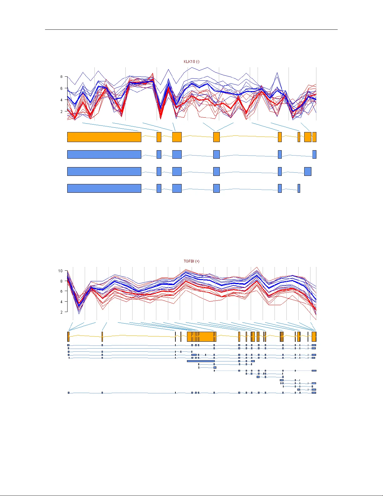
Repro ducible prob e-lev el analysis of the Affymetrix Exon 1.0 ST arra y with R/Bio conductor Maria Ro drigo-Domingo, Rasm us W aagep etersen, Julie Støv e Bødk er, Steffen F algreen, Malene Krag Kjeldsen, Hans Erik Johnsen, Karen Dybkær and Martin Bøgsted Abstract Alternativ e splicing is the p ost- transcriptional pro cess b y whic h a single gene can pro duce m ultiple transcripts and thereb y protein isoforms. The presence of differen t transcripts of a gene across samples can b e analysed b y whole-transcriptome mi- croarra ys. Repro ducing results from published microarra y data represents a challenge due to the v ast amounts of data and the large v ariet y of pre-processing and filtering steps emplo yed b efore the actual analysis is carried out. T o ensure a firm basis for methodological dev elopment where results with new metho ds are compared with previous results it is crucial to ensure that all analyses are completely repro ducible for other researchers. W e here giv e a detailed workflo w on ho w to p erform reproducible analysis of the GeneChip R  Human Exon 1.0 ST Ar- ra y at prob e and prob eset level solely in R /Bio conductor, choosing pack ages based on their simplicit y of use. T o exemplify the use of the prop osed workflo w we analyse differen- tial splicing and differential gene expression in a publicly av ailable dataset using v arious stat- istical metho ds. W e b eliev e this study will pro vide other re- searc hers with an easy w a y of accessing gene ex- pression data at different annotation lev els and with the sufficient details needed for dev eloping their o wn to ols for repro ducible analysis of the GeneChip R  Human Exon 1.0 ST Array . Con tact: maria@math.aau.dk 1 Introduction In the field of microarrays it has traditionally b een difficult to compare new metho ds to metho ds in pub- lished papers as the many metho ds a v ailable for pre- pro cessing, summarizing and filtering mak e it almost imp ossible to work with the exact same data, ev en when the raw data is made av ailable. That is why w e consider reproducible research fundamental as it will facilitate easy 1) revision of papers, 2) access to data and results, 3) communication to other researchers and 4) comparison betw een different metho ds. Re- pro ducible research is gaining relev ance among the scien tific communit y as sho wn by the num b er of pa- p ers published on the sub ject during the last y ears [2, 3, 4]. Ioannidis et al. show ed that the res- ults of only 2 out of 18 published microarra y gene- expression analyses w ere completely reproducible [5]. This is why some authors demand that do cumen t- ation and annotation, database accessions and URL links and ev en scripts with instructions are made pub- licly a v ailable [2]. Journals lik e Biostatistics ha ve ev en app oin ted an Asso ciate Editor for repro ducible researc h, but still treat it as a “desirable goal” rather than a requirement [6]. Setting up a framew ork for repro ducible research necessarily implies working with free and op en-source soft ware as for example R/Bio conductor [7, 8]. Additionally , using Sw eav e [9] (a tool for embedding R co de in L A T E Xdo cumen ts [11]), enables automatic rep orts that can be up dated with output from the analysis. The main to ol in this paper will b e the Biocon- ductor pack age aroma.affymetrix [12] that can analyse all Affymetrix chip types with a (.CDF) Chip Definition File. The num b er of arrays (samples) that can be simultaneously analysed b y aroma.affymetrix is virtually unlimited as the sys- tem requiremen ts are just 1GB RAM, for any op erat- ing system [13]. This pack age is freely av ailable and can easily b e installed into R . The aroma.affymetrix w ebsite www.aroma- project.org is conceiv ed as ref- erence for all the possible microarrays that can b e analysed with aroma.affymetrix , and do es not fo- cus sp ecifically on the analysis of the GeneChip R  Human Exon 1.0 ST Arra y (or exon array in short). P ortable scripts for a fast and basic analysis can b e obtained on request to aroma.affymetrix ’s authors. The analysis of exon array data in R /Bioconductor is not yet standard. There are several pack ages a v ailable, and it can be a tremendous effort for a newcomer to maneuv er b et ween them, and to o vercome the n umerous challenges associated with these pac k ages. This pap er aims to mak e this task easier and to pro vide a quic k reference guide to 1 page 2 of 14 Ro drigo-Domingo et al. aroma.affymetrix ’s do cumen tation. W e also ex- plain ho w to extract data for different statistical ana- lyses and propose a metho d for gene annotation and for gene profile visualization. F or this last step, we use the pack ages biomaRt and GenomeGraphs to an- notate and visualize the transcripts in a genomic con- text. The analysis workflo w presen ted in this pap er is carried out solely in R /Bio conductor, and the pap er is a v ailable as a Swea ve (.Snw) do cumen t that will allo w the reader to repro duce our exact results. The .Sn w do cumen t can also b e con verted in to an R script and executed. The workflo w starts b y reading in the data, follow ed b y background correction and quan tile normalization. W e then explain ho w to obtain tran- script cluster -, prob eset -, and prob e-lev el estimates. Afterw ards, different metho ds for the statistical ana- lysis of differen tial splicing or differen tial gene expres- sion are reviewed. Finally , we mak e a suggestion on ho w to annotate transcript clusters to genes in the lists obtained from the statistical analyses, and how to plot the data including genomic information. T o exemplify the use of the workflo w, an example data- set [14] is analysed along the wa y . 2 Background on alternative splicing Splicing is the post-transcriptional pro cess that gen- erates mature euk aryotic mRNAs from pre-mRNAs b y remo ving the non-coding in tronic regions and join- ing together the exonic co ding regions. F or man y genes, tw o or more splicing ev ents tak e place during maturation of mRNA molecules resulting in a cor- resp onding num b er of alternatively spliced mRNAs. These mature mRNAs translate into protein isoforms differing in their amino acid sequence and ultimately in their bio c hemical and biological properties [15, 16]. Alternativ e splicing is one of the main tools for gen- erating RNA div ersity , contributing to the diverse rep ertoire of transcripts and proteins [16, 17]. It is kno wn that 92-94% of multi-exon human genes are alternativ ely spliced and that 85% of those ha ve a minor isoform frequency of at least 15% [18, 19]. In our case we will fo cus on the detection of differential splicing b et ween groups, as for instance tissue t yp es, or healthy vs. diseased samples. The exon arra y was presented in Octob er 2005 as a to ol for the analysis and profiling of whole- transcriptome expression [20, 21, 22]. T o in terrogate eac h p oten tial exon with at least one prob eset, the exon arra y con tains ab out 5.6 million prob es grouped in to more than 1.4 million prob esets (most prob esets consisting of 4 probes), which are further group ed in to 1.1 million exon clusters, or collections of o ver- lapping exons. Finally , exon clusters are group ed into o ver 300.000 transcript clusters to describ e their re- lationship, as for example shared splice sites or ov er- lapping exonic sequences. Each gene is cov ered, on a verage, by 40 prob es in terrogating regions located along the entire gene [23]. This prob e positioning aims at providing b etter estimates of gene expression lev els than previous arrays, and allows for the study of differential splicing [24] and differen tial gene ex- pression based on summarized exon expression. The exon array has three lev els of annotation for the in terrogated transcript clusters: c or e, extende d and ful l [25]. Core transcript clusters are supp or- ted by the most reliable evidence such as RefSeq transcripts and full-length mRNAs [26] and a core transcript cluster is roughly a gene [27]; the exten- ded level contains the core transcript clusters plus cDNA-based annotations [28] and the full level con- tains the t wo previous lev els plus ab-initio , or al- gorithmic, gene predictions [29]. It is worth noting that aroma.affymetrix enables the analysis at the three levels of annotation mentioned ab ov e, and also that it pro vides intensit y estimates for probes, prob e- sets and transcript clusters, allo wing for a v ariety of options for the analysis. 3 W orkflo w Our workflo w for the analysis of exon array data starts setting up the required folder structure for aroma.affymetrix . The data is then preprocessed and summarised at transcript cluster and/or probe- set level. Next, transcript clusters are analysed with sev eral statistical models to detect differential expres- sion or splicing and the transcripts of interest are an- notated and visualised at the end, see Figure 1. In the co de, places where user input is needed are marked b y “***”, and places where the user can choose whether to mo dify parameters are mark ed b y “**”. T o exemplify the use of the tutorial we ha ve used Affymetrix’s colon cancer data set [14], consisting of a collection of paired samples of colon tumour tissue and adjacen t normal tissue from 10 patients and a v ailable at http://www.affymetrix.com/support/ technical/sample_data/exon_array_data.affx . According to Affymetrix’s website, the RNA samples are from a commercial source. This dataset has b een used in a n umber of pap ers to ev aluate the p erform- ance of differen t analysis metho ds [30, 31, 32, 33] and a n um b er of genes ha ve b een v alidated to present differen tial splicing or not [14]. The analysis w as done in R v ersion 2.15.1 (32 bit). Start by installing and loading aroma.affymetrix in R and loading the other libraries required: Repro ducible exon array analysis with R/Bio conductor page 3 of 14 Figure 1: Flo wc hart for an analysis with aroma.affymetrix , read coun ter-clo c kwise starting in upper left corner: 1. and 2. folder structure set-up including library , annotation and .CEL files, 3. data pre-pro cessing and summarization, 4. extraction of in tensities at transcript cluster, probeset and probe level, including filtering recommended by Affymetrix, 5. statistical analysis of differentially expressed or spliced transcript clusters and 6. annotation and visualization of transcript cluster profiles. Blue b o xes represent parts of the analysis implemented in aroma.affymetrix , y ellow and green b oxes are part of the co de provided in this pap er, and purple b oxes represen t user-input needed. Output pro duced at sev eral steps is sa ved in user-c hosen ” output.folder ” and represen ted by a star shap e in the workflo w. A n um b er of folders are automatically generated b y aroma.affymetrix - represen ted b y a faded yello w rectangle in 3. -, our w orkflow do es not make use of the con tents of such folders. page 4 of 14 Ro drigo-Domingo et al. > source("http://aroma-project.org/hbLite.R") > hbInstall("aroma.affymetrix") > require(aroma.affymetrix) > require(biomaRt) > require(GenomeGraphs) 3.1 Setting up the structure and files for the analysis w orkflo w This section corresp onds to steps 1. and 2. in Figure 1. The first step is to create the folder structure: under a main folder of our c hoice - “ myworkingDirectory ” - we will cre- ate the “ rawData ” and “ annotationData ” folders, whic h will b e common to all aroma.affymetrix pro jects. Inside “ annotationData ”, the subfolder “ chipTypes ” will contain one subfolder per chip t yp e, with the exact name of the .CDF file provided b y Affymetrix, “ HuEx-1 0-st-v2 ” in our case. Inside this folder we will sav e any library and annotation files that migh t b e needed. Besides, the “ myDataSet ” folder will b e created under “ rawData ” to store .CEL files. These files are the output of a microarray ex- p erimen t and con tain the result of the in tensity calcu- lations per prob e or pixel. Note that the microarray exp erimen t produces one .CEL file p er array and that one array analyses one sample. Affymetrix sometimes refer to their microarra ys as “c hips”. Note also that w e need one “ myDataSet ” folder p er exp erimen t and that “ myDataSet ” will b e added as a tag at the end of the aroma.affymetrix output. > # *** user-defined working directory > wd <- "myWorkingDirectory" > # *** user-defined data set name > ds <- "myDataSet" In the second step we sav e our library (Chip Definition File (.CDF) in our case) and .CEL files in the corresp onding folders. Affymetrix’s unsupp orted .CDF files can b e do wnloaded from http://www.affymetrix.com/Auth/support/ downloads/library_files/HuEx- 1_0- st- v2.cdf.zip , note that registration is needed. F or the exon array , Elizab eth Purdom has created a n umber of binary .CDF files based on Affymetrix’s text .CDF file [13] that are faster to query and more memory efficien t. Such binary .CDF files for core, extended and full sets of prob esets can b e do wnloaded from http://aroma- project.org/node/122 . In the example b elo w w e use the custom aroma file for core transcript clusters, whic h migh t be up dated in the future. Our original .CEL files will be copied from the user-sp ecified “ myCELfileDirectory ” into the exon “ rawData ” subfolder (the co de is part of the .Sn w v ersion of this pap er). The desired output folder sp ecified in “ output.folder ” should exist in adv ance. > # ** download user-defined library file > library.file <- + paste(annotation.data.exon, + "HuEx-1_0-st-v2,coreR3,A20071112,EP.cdf", + sep = "/") > download.address <- + "http://bcgc.lbl.gov/cdfFiles/" > file <- paste("HuEx-1_0-st-v2,A20071112,EP", + "HuEx-1_0-st-v2,coreR3,A20071112,EP.cdf", + sep = "/") > custom.cdf <- + paste(download.address, file, sep = "") > download.file(url = custom.cdf, + destfile = library.file, + mode = "wb", quiet = FALSE) > # *** user-defined directory containing .CEL files > cel.directory <- "myCELfileDirectory" > # *** user-defined output folder > output.folder <- "output.folder" Besides, the sample information should b e sa ved in a tab separated file with column names celFile , replicate , and treatment containing .CEL file name (without .CEL), replicate identi- fier and treatmen t name, resp ectiv ely . This file should be called ”SampleInformation.txt” and it will b e copied from the user-sp ecified directory in to the " \ rawData \ myDataSet \ HuEx-1 0-st-v2" folder (whic h will also contain the .CEL files) after it has b een created. The sample information file for the colon cancer example is attac hed as an additional file. > sample.info <- + read.table(file = paste(raw.data.exon, + "SampleInformation.txt", sep = "/"), + sep = "\t", header = TRUE) Finally , NetAffx transcript clusters’ and prob esets’ annotation files should b e sav ed in “ annotationData/chipTypes/ ” “ HuEx-1 0-st-v2 ”. W e ha ve used release 32, which was most up to date at the time of writing and we do wnloaded files “HuEx-1 0-st-v2.na32.hg19.transcript.csv.zip” and “HuEx-1 0-st-v2.na32.hg19.prob eset.csv.zip” from http://www.affymetrix.com/estore/browse/products. jsp?productId=131452&categoryId=35676&productName= GeneChip- Human- Exon- ST- Array#1_3 , T e chnic al Do cu- mentation tab, under NetAffx Annotation Files . The extracted .csv files should be con verted in to .Rdata files for querying them faster in the future. Note that the n umber of lines to skip migh t differ for future annotation files. > transcript.clusters.NetAffx.32 <- + read.csv(file = paste(annotation.data.exon, + "HuEx-1_0-st-v2.na32.hg19.transcript.csv", + sep = "/"), skip=24) > probesets.NetAffx.32 <- + read.csv(file = paste(annotation.data.exon, + "HuEx-1_0-st-v2.na32.hg19.probeset.csv", + sep = "/"), skip=23) Repro ducible exon array analysis with R/Bio conductor page 5 of 14 3.2 Data pre-pro cessing and sum- marization to prob eset/transcript cluster level After defining c hip t yp e and dataset, bac kground cor- rection and quantile normalization are carried out as sho wn in Figure 1, step 3. In these pre-pro cessing steps, it is p ossible to use either Affymetrix’s ori- ginal .CDF file, the .CDF files provided b y the aroma pro ject (the file for core transcript clusters in our example), or a .CDF file created b y the user. The summarization step, how ever, must b e done us- ing one of the custom .CDF files a v ailable at the aroma.affymetrix pro ject w ebsite. Bac kground correction as defined by Ir- izarry [34] and quantile normalization are p er- formed by the RmaBackgroundCorrection() and QuantileNormalization() functions, resp ectively . The raw, background corrected and quan tile nor- malized probe intensities can b e visualized using the plotDensity() function applied to the cor- resp onding ob ject. Summarization is done with the ExonRmaPlm function [35]. The parameter mergeGroups determines whether to summarize at transcript level ( TRUE ) or prob eset level ( FALSE ). All the functions describ ed automatically create subfolders such as “plmData” or “prob eData” inside “ myWorkingDirectory ”. A more detailed version of this co de with interesting comments ab out the c hoice of .CDF and possibilities for qualit y con trol is av ailable at http://www.aroma- project.org/ vignettes/FIRMA- HumanExonArrayAnalysis . > chipType <- "HuEx-1_0-st-v2" > # ** user-defined .CDF file: change tags parameter > cdf <- AffymetrixCdfFile$byChipType(chipType, + tags = "coreR3,A20071112,EP") > cs <- AffymetrixCelSet$byName(ds, cdf = cdf) > > # background correction > bc <- RmaBackgroundCorrection(cs) > csBC <- process(bc, verbose = verbose) > > # quantile normalization > qn <- QuantileNormalization(csBC, + typesToUpdate = "pm") > csN <- process(qn, verbose = verbose) > > # summarization > # transcript cluster level > plmTr <- ExonRmaPlm(csN, mergeGroups = TRUE, + tag = "coreProbesetsGeneExpression") > # probeset/exon level > plmEx <- ExonRmaPlm(csN, mergeGroups = FALSE, + tag = "coreProbesetsExonExpression") 3.3 Extraction of in tensity estimates The aroma.affymetrix do cumentation fo cuses on analyses at the prob eset and transcript cluster levels. The resp ective in tensities are obtained b y apply- ing the function getChipEffectSet() to the tran- script or prob eset plm ob jects ( plmTr and plmEx , resp ectiv ely) and then extracting the correspond- ing dataframes. How ev er, it is also p ossible to ex- tract the bac kground corrected and quantile nor- malized in tensities of all prob es using the function getUnitIntensities . While plmTr is suitable for the FIRMA analysis (3.4), plmEx is w ell suited for prob eset-lev el analysis. F or the linear mo del ana- lysis describ ed in Section 3.4 we ha ve created one list of dataframes containing prob e in tensities p er tran- script cluster, and another list of dataframes con tain- ing prob eset in tensities per cluster (code included in .Sn w). > # extract a matrix of gene intensities > cesTr <- getChipEffectSet(plmTr) > trFit <- extractDataFrame(cesTr, addNames=TRUE) > # extract a matrix of probeset intensities > cesEx <- getChipEffectSet(plmEx) > exFit <- extractDataFrame(cesEx, addNames=TRUE) > # extract a list of probe intensities per gene > unitIntensities <- readUnits(csN, verbose=verbose) The high n umber of transcript clusters analysed in com bination with the usually small num b er of c hips tends to cause a high n umber of false p ositiv es [25]. In order to reduce the n umber of false p ositiv es, Affy- metrix recommends to perform detection abov e bac k- ground (DABG) [36] on the dataset prior to the ana- lysis [25]. The D ABG pro cedure is not implemen ted in aroma.affymetrix , so we decided to follow the pro cedure describ ed in [30] and use 3 as a threshold for the probeset intensit y , so that probesets with a log 2 in tensity b elo w 3 will b e marked as absen t. Ex- cept for this change, w e follo wed the guidelines pro- p osed in [25] to remo ve absent transcript clusters and prob esets, where neither probesets that are absen t in more than half of the samples of a group nor tran- script clusters with more than half of the prob esets absen t are analysed. Besides this filtering based on expression levels, another filtering that remo ves prob esets presenting cross-h ybridization is also advisable [25]. Cross- h ybridising probesets are iden tified in file ”HuEx-1 0- st-v2.na32.hg19.prob eset.csv” and remo ved. Affyme- trix recommends to filter them out after the analysis, but we ha ve decided not to include them in the ana- lysis in order to narrow down the n umber of prob e- sets/transcript clusters to in vestigate. The filtering pro cedure is part of the .Snw file. In our example, where we analysed only core prob esets, 136233 prob esets out of 284258 were deemed presen t b y our filter, and the num b er of transcript clusters to analyse (present in b oth samples) was reduced from 18708 to 8401. page 6 of 14 Ro drigo-Domingo et al. 3.4 Statistical analysis In this section we giv e an ov erview of mo del-based statistical methods av ailable for the analysis of differ- en tial splicing and suggest a metho d for the analysis of differential gene expression. 3.4.1 Differential splicing The analyses carried out in this pap er are model- based approaches, and the analysis of differential spli- cing is done genewise. The mo dels we use are exten- sions of the linear mo del by Li and W ong [37] y pt = α p + β t + ε pt , (1) where y pt is the intensit y measure of probe p for treat- men t t , α p is a prob e affinity term, β t is the gene-lev el estimate for treatmen t t , and ε pt is the error term. ANOSV A (Analysis of Splicing V ariation) was presen ted b y Cline et al. [38] and is a tw o-wa y AN- O V A mo del with prob eset and treatmen t as factors: y pet = µ + α e + β t + γ et + ε pet , (2) where y pet is the intensit y measure of prob e p in prob eset e and treatmen t t , the o verall mean µ is the baseline level of all prob es in all experiments, and α e and β t are the prob eset and treatment effects. The in teraction term γ et tells whether the effect of the prob eset dep ends on the treatmen t and is therefore k ey to the detection of differential splicing. The mo del in (2) can be extended to include ran- dom effects associated to replications from the same individual, r : y petr = µ + α e + β t + γ et + I r + C tr + ε petr , (3) where I r is the random effect of eac h individual r and C tr is the random chip effect. The error terms ε petr are i.i.d. N(0 , σ 2 )-distributed. Under the n ull-hypothesis of no differential spli- cing, the γ et ’s will all b e zero, therefore we consider the test statistic t et = ˆ γ et ˆ σ , where ˆ γ et is the estimate for γ et , and ˆ σ is the stand- ard error of ˆ γ et . Large v alues will b e critical for the n ull hypothesis. Under the mo del assumptions, t will follo w a t N − T · ( n e + R − 1) distribution [39, Chap. 5], with N the total num b er of observ ations p er tran- script cluster, T the num b er of treatmen ts, n e the n umber of prob esets in the transcript cluster and R the num b er of individuals. F or each gene, the smal- lest p -v alue from the ab o ve t -tests is regarded as a measure of confidence that the gene is differentially spliced across the experimental conditions [38]. The in teraction estimates and v ariances and thus the test statistics are contrast-dependent, so c ho osing a differ- en t con trast will alter the gene lists. In our analysis, w e hav e used the sum contrast a v ailable in R , where parameter estimates are cen tred around zero. A pac k age in R for fitting linear and generalized lin- ear mixed-effects mo dels is lme4 [52]. Linear mixed- effects mo dels can also b e analysed using lm , whic h is faster but requires a balanced design. In our ex- ample dataset w e use lm to fit the model in equa- tion (3) to the probe level estimates obtained us- ing unitIntensities() from aroma.affymetrix to 8075 multiexonic transcript clusters. Here, we only sho w the co de corresponding to equation (3), the rest of the code is part of the .Snw file. > # ** user-defined parameters for linear model > lm <- + lm(intensity ˜ probeset + treatment + + C(probeset:treatment, contr.sum) + + replicate/treatment) > n.probesets <- length(unique(dataframe$probeset)) > main.effects <- + 1 + (n.probesets - 1) + + (length(unique(dataframe$treatment)) - 1) > DS.parameters <- (n.probesets - 1) * + (length(unique(dataframe$treatment)) - 1) > p.t <- + min(summary(lm)$coefficients[(main.effects+1): + (main.effects + DS.parameters),"Pr(>|t|)"]) Although the v ast ma jority of prob esets con tain 4 prob es, transcript clusters con taining probesets with less than 4 prob es will giv e rise to an un balanced design. Nevertheless, the t -distribution is almost a normal distribution for long transcript clusters so the un balanced design does not ha ve an y practical im- plications. F or shorter transcript clusters, ho wev er, an unbalanced design might be a problem. The top 10 most differen tially spliced genes, sor- ted b y the minimum p -v alue of their t -tests, app ear in T able 1a. The gene ZAK was v alidated as dif- feren tially spliced in [14]. See Figure 2 for the pro- file plot of KLK10 , where the thick lines representing the mean intensit y in each group ha ve been plotted for easing the in terpretation. Note that there is one measuremen t per prob e in each prob eset, typically 4 prob es p er prob eset. How to obtain suc h plots is de- scrib ed in Section 3.5 b elo w. The genes in Figures 2, 3, 4 and 6 were chosen because they span o ver a shorter genomic region and show a more clear picture of the relationship b etw een prob esets and exons than the other genes in the lists of top 10 genes. A slight v ariation of ANOSV A is the prob eset- mo del as implemented in P artek [40] (note that the prob e subscript p has been remo ved): y etr = µ + α e + β t + γ et + I r + C tr + ε etr . (4) F or the prob eset-lev el ANOSV A we used the prob eset level estimates obtained by affyPLM(..., Repro ducible exon array analysis with R/Bio conductor page 7 of 14 mergeGroups = FALSE) . After filtering for non- presen t or cross-hybridising prob esets, and absent transcript clusters, w e w ere left with 9494 transcript clusters to study . These clusters are sorted accord- ing to the minimum p -v alue of the individual t -test scores for differential splicing, and the top 10 genes obtained app ear in T able 1b. T he genes MMP11, ZAK and COMP are in the top 10 genes for b oth the ANOSV A prob e and the ANOSV A prob eset models. Gene TGFBI appears in Figure 3. FIRMA (Finding Isoforms using Robust Multi- c hip Analysis) was first in tro duced by Purdom et al. [30] for the exon arra y . In presence of differential spli- cing the mo del in (1) will not fit and this will show up in the residuals. The linear mo del used is the follo wing: y petr = α p + β tr + ε petr , (5) with α p the probe affinity , β tr the gene-lev el effect for c hip tr and the error terms ε petr are i.i.d. N(0 , σ 2 )- distributed. Note that in contrast to the mo del in (3) we do not compute an o verall gene-lev el estimate, but a gene-lev el estimate per c hip. As in model (1), there is no treatment/probeset in teraction term, so differential splicing is analysed prob eset wise, using the residuals p er prob eset e : r petr = y petr − ( ˆ α p + ˆ β tr ) , (6) p = 1 , . . . n e , t = 1 , . . . , T , r = 1 , . . . , R where ˆ α p and ˆ β tr are the estimates of α p and β tr . The median of the standardized residuals p er prob eset per c hip is chosen as score statistic: F e ( tr ) = median p =1 ,...,n e  r petr MAD  . (7) The standardization with the me dian absolute de- viation (MAD) of the residuals p er gene mak es the scores comparable across transcript clusters. The FIRMA scores are extracted from the plmTr ob ject obtained in Section 3.2. All probesets and transcript clusters w ere analysed b y FIRMA, since it is part of the default aroma.affymetrix w orkflow. > firma <- FirmaModel(plmTr) > fit(firma, verbose = verbose) > fs <- getFirmaScores(firma) > firma.scores <- extractDataFrame(fs) After obtaining the FIRMA scores p er prob eset per sample, w e pro ceeded as describ ed in [30]: 1) F or each prob eset w e took the difference of FIRMA scores for eac h of the 10 pairs of normal/cancer samples and 2) calculated the mean of the 10 differences p er prob e- set. Then 3) we ranked the prob esets according to their absolute mean difference: as the scores are com- parable across transcript clusters, larger a verage dif- ferences b et w een the normal and cancer samples will p oin t at exons more differentially spliced b etw een the t wo conditions. The resulting list was filtered to k eep only prob esets and transcript clusters that has passed the filter described in 3.3 ab o ve, the co de is part of the .Sn w file. In order to get a gene list instead of a prob eset list as in [30] we mapped prob esets to tran- script clusters and then selected the top 10 genes on the list, see T able 1c. The profile plot of gene LGALS4 appears in Figure 4. The very high av erage difference for this gene is due to a FIRMA score of 830030.8 at prob eset 3861578 corresp onding to the tumour sample of replicate 7. Out of 14 genes in vestigated for differen tial splicing in [14, T able 1], 10 passed our filtering procedure and w ere analysed for differential splicing: A CTN1, VCL, CALD1, SLC3A2, COL6A3, CTTN, FN1, MAST2, ZAK and FXYD6 . The gene ZAK app ears in the top 10 genes from ANOSV A prob e and ANOSV A prob e- set, but a plot is not produced automatically by the co de b ecause ZAK is not recognised b y BioMart. In- stead, we lo ok ed the gene up in PubMed obtaining the Ensembl ID: ENSG00000091436, and used this to plot the gene, see Figure 5. The gene COL6A3 app ears among the top 100 genes for the ANOSV A prob e and the ANOSV A prob eset metho ds. Gene AC TN1 is among the top 100 genes for ANOSV A prob eset and it is also the first of Gardina’s genes to app ear in the filtered FIRMA list, at p osition 154. 3.4.2 Differential gene expression In this section w e analyse differen tial gene expres- sion using prob e lev el data. W e study tw o types of transcript clusters: 1) the ones not included in the ANOSV A prob e analysis ab o ve (with only one prob eset or not presen t in b oth normal and cancer groups) and 2) the ones not showing differential spli- cing (ANOSV A prob e p -v alue ab ov e 0.1). The ana- lysis of group 2) is based on the hierarc hical principle: only look for significant main effects (differential ex- pression in this case) among those transcript clusters with no significan t in teraction terms (differential spli- cing) [46, p. 427]. In total, we analysed 16231 tran- script clusters. W e fit the following linear model to those transcript clusters: y petr = µ + α e + β t + I r + C tr + ε petr , (8) where β t is the gene level treatmen t effect, α e is a parameter that captures prob esets expressed ab o ve or below the ov erall transcript cluster lev el and I r and C tr are random effects for patient and chip, re- sp ectiv ely . > aov <- + aov(intensity ˜ probeset + treatment + + Error(replicate + replicate:treatment)) page 8 of 14 Ro drigo-Domingo et al. Gene sym b ol min p -v alue MMP11 2 . 98 e − 10 SOX9 2 . 59 e − 09 FO XQ1 6 . 38 e − 09 KLK10 3 . 84 e − 08 SYNM 4 . 53 e − 07 PHLDA1 4 . 85 e − 07 ZAK 4 . 89 e − 07 SNTB1 5 . 33 e − 07 COMP 6 . 85 e − 07 XPOT 7 . 87 e − 07 (a) Model: ANOSV A prob e. Gene sym b ol min p -v alue SOX4 9 . 07 e − 15 MMP11 9 . 48 e − 14 ZAK 4 . 40 e − 13 FO XQ1 5 . 98 e − 13 TGFBI 4 . 83 e − 12 UBAP2L 8 . 17 e − 12 COMP 2 . 87 e − 11 SLC2A1 4 . 16 e − 11 CDH11 4 . 19 e − 10 CPXM1 4 . 47 e − 10 (b) Model: ANOSV A prob eset. Gene sym b ol Average difference LGALS4 83000 . 0 HMGCS2 82 . 9 RPS6KA1 31 . 8 MUC13 28 . 2 RPL35 24 . 5 RPL35A 18 . 8 SLC39A14 18 . 2 TGFBI 16 . 2 COL23A1 15 . 5 SFT2D2 14 . 2 (c) Model: FIRMA. T able 1: T op 10 differen tially spliced genes from the mo dels describ ed in 3.4.1. T ables (a) and (b) sho w genes with minum um p -v alues, table (c) shows genes with their top scores. Genes highlighted in gray ap- p ear in Figures 2, 3, 4 and 5. > p.F <- + summary(aov)$"Error: Within"[[1]]["treatment", + "Pr(>F)"] The null hypothesis is that the gene expression is the same in all groups. The top 10 genes, with ad- justed p -v alues app ear in T able 2. The metho d used for adjusting the p -v alues was Benjamini-Ho c hberg’s correction [47] using the function p.adjust(..., method = "BH") . Only 80 out of 159 genes ap- p earing in Gardina’s list of genes up- and down- regulated in tumour [14, Additional file 1] passed our filters and were analysed for differential gene expres- sion. Among those analysed, the genes CLDN1, SST, MUSK, KIAA1199 and SLC30A10 were in the top 100. The gene BEST4 is shown in Figure 6. This gene is down-regulated in tumour (blue) compared to normal (red) samples. The thic ker lines represent the mean expression lev els in the tw o groups. 3.5 Gene annotation and visualization W e c hose to annotate transcript clusters to genes using the NetAffx transcript cluster annotation release 32 sp ecified in Section 3.1 using the AnnotateGenes() function. Some transcript clusters presen t unsp ecific annotation and hav e sev eral pos- Gene symbol p -v alue LAR GE 0 . 00287 IL6R 0 . 00847 RXR G 0 . 00847 BAI3 0 . 00968 C1orf175 0 . 01090 GRIK3 0 . 01090 BEST4 0 . 01090 K CNN3 0 . 01090 PLEKHH2 0 . 01090 HO XD10 0 . 01090 T able 2: T op 10 differentially expressed genes from (8) with corrected p -v alues. Gene BEST4 , high- ligh ted in gray , app ears in Figure 6. sible associated gene names. W e ha ve decided to re- mo ve such clusters from our output as w e cannot map them uniquely to a gene and afterwards interpret the result according to the gene structure. After gene annotation, the user can select genes for visual insp ection. Visual insp ection of candidates for differen tial splicing is recommended by Affymetrix as a w ay to identify possible false p ositiv es [25]. Plots of gene profiles with integrated genomic information are obtained using the biomaRt [48] and GenomeGraphs [49] pack ages in Bioconductor. W e use bioMart to connect to the latest version of the Homo Sapiens dataset in Ensembl [50] (Ensembl genes 68, GRCh37.p8 at the time of writing) and re- triev e genes by their HGNC symbol [51]. Gene and exon structures are imp orted from Ensembl. Gene and Exon ob jects are created by makeGene() and makeTranscript() from GenomeGraphs . W e store expression data and probeset start and stop p osi- tions in an ExonArray ob ject by makeExonArray() . The final plot is created passing a list with the ob jects created to the gdPlot(list(exon, gene, transcript,...)) function. Our plots sho w on top the gene HGNC symbol fol- lo wed by (+) for genes on the forw ard strand and b y (-) for those on the rev erse strand. Belo w, the plot of prob eset in tensities app ears with vertical lines de- limiting prob esets. Note that for models based on prob e-lev el data (ANOSV A prob e, FIRMA and dif- feren tial expression), the in tensities of all prob es in the prob eset (1 to 4) are sho wn. Samples from the same treatment group appear in the same colour, red for normal samples and in blue for tumour samples in this case. Immediately after the profile plot, the gene mo del retriev ed from Ensem bl is sho wn in orange, follo wed b y the possible transcript model(s) in blue. The gene mo del consists of the exons that app ear in all p ossible transcript mo dels. Exons (b oxes) in the Repro ducible exon array analysis with R/Bio conductor page 9 of 14 gene mo del are link ed by blue lines to the prob esets ab o v e, indicating whic h prob eset(s) interrogate whic h exon. See Figures 2 to 6. 4 Discussion The aim of this pap er w as to giv e a tutorial on ho w to perform a complete and reproducible analysis of exon array data in R /Bio conductor. W e hav e w orked with three pac k ages: aroma.affymetrix , biomaRt and GenomeGraphs to go from .CEL files to intens- it y data, s tatistical analysis, annotation and visualiz- ation. The pac k ages were chosen for their flexibilit y and easy of integration. W e believe that our work- flo w cov ers a n umber of analysis v arian ts for the exon arra y , including differen tial splicing analysis at prob e and prob eset-lev el and differen tial expression analysis at prob e level, and gives the user the opp ortunit y to fo cus on all or only some of the asp ects of the data analysis. W e make our en tire co de av ailable so that other researc hers can use it as it is or adapt it to their needs. Differen t Bio conductor pack ages could ha ve been used in some of the analysis steps. F or example, xmapcore [54] provides annotation data and cross- mappings b et ween genetic features as transcript clusters or exons and Affymetrix prob esets. This pac k age, ho wev er, requires the separate installation of a MySQL database, whic h makes this a more com- plex alternativ e than the one w e ha ve chosen. The xps pack age [55] could ha ve b een used for data pre- pro cessing and summarization, but it requires the in- stallation of the ROOT framework [56], and a certain lev el of understanding of R OOT files and ROOT trees is recommended. Our workflo w does not require an y prior kno wledge b ey ond R /Bio conductor. Other free soft ware includes BRB-Arra y T o ols [57], based on R , C, F ortran and Ja v a, with an Excel fron t end, and dChip [58], whic h is written in Visual C ++ and de- v elop ed for Windows - though some users hav e b een able to run it on Mac and Unix computers. A previous pap er on exon arrays [24] suggests a pragmatic approach and do es the analysis piecewise starting with Affymetrix P ow er T o ols (APT) and then exp orting the data to R . W e recognise this is a fix for the lack of straightforw ard pac k ages for deal- ing with the exon array in Bioconductor. How ever, it implies working with several pieces of softw are so w e do not find it fit for repro ducible researc h. Li- censed softw are, lik e Partek [40] or GeneSpring GX [59], has b een used in other studies [60, 22]. In con- trast to licensed softw are, R /Bio conductor is free and a v ailable for an yone, it allo ws the user to control most analysis options and it enables customizable and repro ducible analyses that are more easily re- view ed. Still, the aroma.affymetrix pack age does not pro vide the sp eed of Affymetrix Po wer T o ols or the licensed softw are, and it requires more user input. Nev ertheless, with this code and minimal user input, an y dataset can be analysed regarding differen tial ex- pression at prob e level and differential splicing using the ANOSV A mo del. Differen tial gene expression could ha ve b een ana- lysed using the gene level estimates obtained from the plmTr ob ject in other R pack ages such as limma [53]. Another extension of the w orkflow could include a general analysis strategy of the FIRMA scores, which in this study w as tailor-made for a t wo-treatmen t scenario. Besides, the profile plots we obtained with GenomeGraphs , though highly informative, are diffi- cult to in terpret for genes spanning ov er a long gen- omic region, as for example TGFBI in Figure 3 and ZAK in Figure 5. In the future, it would b e inter- esting to study the flexibility of the output imp orted from Ensem bl and, for example, remo ve the in tronic regions from the gene and transcript mo dels. Ac kno wledgements/Author declaration The authors would like to thank Henrik Bengts- son for helpful answers and comments regarding aroma.affymetrix . The authors w ould also lik e to thank Hang Phan and Anders Ellern Bilgrau for help- ful discussions and ideas about code implemen tation and data plotting. MRD designed and implemen ted the w orkflow, analysed data and drafted the man uscript. R W as- sisted in pap er drafting and statistical mo delling and in terpretation. JSB, SF and MKK tested the w ork- flo w. JSB, MKK, HEJ and KDS assisted with data in terpretation and participated in pap er drafting. MB conceived and tested the workflo w, assisted in man uscript drafting and co ordinated the work. All authors read and appro ved the final man uscript. References [1] Hothorn T and Leisc h F. Case studies in repro- ducibilit y . Briefings in Bioinformatics , 2011. [2] Baggerly KA. Disclose data in all publications. Natur e , 2010, 467. 149-155. [3] Baggerly KA and Co om b es KR. Deriving c hemosensitivity from cell lines: F orensic bioin- formatics and repro ducible researc h in high- throughput biology . The A nnals of Applie d Stat- istics , 2009, 3:1309–1334. [4] Co ombes KR, W ang J, and Baggerly KA. Mi- croarra ys: retracing steps. Natur e Me dicine , 2007, 13. Corresp ondence. page 10 of 14 Ro drigo-Domingo et al. Figure 2: Profile plot of gene KLK10 with the gene model and p ossible transcripts retriev ed from Ensembl [50]. The (-) next to the gene name indicates that it is on the reverse strand. The mean in tensities of each group are plotted with a thick er line. Exons 5 (mapp ed b y prob esets 4 and 5) and 8 (mapp ed by probeset 9), counted from the 5’ end, seem to b e higher expressed in tumour samples (blue) than in normal (red). Figure 3: Profile plot of TGFBI with the gene mo del and transcripts retrieved from Ensem bl [50]. The gene is on the forward strand as indicated by (+) next to its name. The mean in tensities of eac h group are plotted with a thick er line, note that only one estimate is plotted by probeset, it corresp onds to the estimate computed by ExonRmaPlm(..., mergeGroups=FALSE) . Here, it seems lik e the tumour samples (blue) present increased expression from exon 3 until the end of the transcript, with resp ect to normal (red) samples. Given that TGFBI is on the forward strand and that the difference is at the b eginning of the transcript, w e might b e observing a case of alternative promoter usage. Repro ducible exon array analysis with R/Bio conductor page 11 of 14 Figure 4: Profile plot of gene LGALS4 with the gene model and transcripts retrieved from Ensembl [50], the gene is on the reverse strand. In terestingly , this gene only has one transcript. W e migh t then b e facing a nov el splicing ev ent or, more likely , a false p ositiv e detected b y the metho d. Figure 5: Profile plot of gene ZAK with the gene mo del and transcripts retrieved from Ensembl [50]. There seems to b e a differen tial splicing even t identified b y prob esets 5 and 6 (counted from the 3’ end of the gene), corresp onding to exons 3 and 4 from the 3’ end. page 12 of 14 Ro drigo-Domingo et al. Figure 6: Profile plot of gene BEST4 , which is on the reverse strand, with the gene mo del and transcripts retriev ed from Ensembl [50]. The gene is under expressed in tumour (blue) compared to normal (red) samples. The thin lines are the expression levels for eac h sample, while the thick er lines represent the mean in tensities in each of the tw o groups. [5] Ioannidis JP , Allison DB, Ball CA, et al. Rep eat- abilit y of published microarray gene expression analyses. Natur e Genetics , 2009, 41:149–155. [6] Peng RD. Repro ducible research and Biostatist- ics . Biostatistics , 2009, 10:405–408. [7] R Dev elopment Core T eam . R: A L anguage and Envir onment for Statistic al Computing . R F oundation for Statistical Computing, Vienna, Austria, 2011. [8] Gentleman R C, Carey VJ, Bates DM, et al. Bio conductor: Op en soft ware dev elopment for computational biology and bioinformatics. Gen- ome Biolo gy , 2004, 5:R80. [9] Leisch F. Swea ve: Dynamic Generation of Statistical Rep orts Using Literate Data Ana- lysis. In H¨ ardle W olfgang and R¨ onz Bernd, edit- ors, Compstat 2002 — Pr o c e e dings in Computa- tional Statistics , pages 575–580. Physica V erlag, Heidelb erg, 2002. [10] Ramsey N. Noweb home p age , Nov ember 2012. h ttp://www.cs.tufts.edu/ ∼ nr/no web/. [11] Lamp ort L. L A T E X: A Do cument Pr ep ar ation System . Addison-W esley Pub. Co, 2 edition, 1994. [12] Bengtsson H, Simpson K, Bullard J, et al. aroma.affymetrix: A generic framework in R for analyzing small to very large Affymetrix data sets in b ounded memory . T ec hnical Report 745, Departmen t of Statistics, Universit y of Califor- nia, Berkeley , 2008. [13] Bengtsson H, Bullard J, Hansen K, et al. A r oma pr oje ct , Jan uary 2012. http://www.aroma- pro ject.org/. [14] Gardina PJ, Clark T A, Shimada B, et al. Altern- ativ e splicing and differential gene expression in colon cancer detected b y a whole genome exon arra y . BMC Genomics , 2006, 7. [15] Black DL. Mec hanisms of alternative pre- messenger RNA splicing. A nnual R eviews of Bio chemistry , 2003, 72:291–336. [16] Hallegger M, Llorian M, and Smith CWJ. Al- ternativ e splicing: global insights. The FEBS journal , 2010, 277(4):856–866. [17] Licatalosi DD and Darnell RB. RNA pro cessing and its regulation: global insights in to biolo- gical netw orks. Natur e R eviews Genetics , 2010, 11(1):75–87. [18] Pan Q, Shai O, Lee LJ, et al. Deep survey- ing of alternative splicing complexity in the hu- Repro ducible exon array analysis with R/Bio conductor page 13 of 14 man transcriptome b y high-throughput sequen- cing. Natur e Genetics , 2008, 40:1413–1415. [19] W ang ET, Sandb erg R, Luo S, et al. Alternat- iv e isoform regulation in h uman tissue transcrip- tomes. Natur e , 2008, 456:470–476. [20] Clark T A, Sch weitzer AC, Chen TX, et al. Dis- co very of tissue-specific exons using comprehens- iv e h uman exon microarrays. Genome Biolo gy , 2007, 8. [21] Suzuki H, Osaki K, Sano K, et al. Comprehens- iv e analysis of alternative splicing and function- alit y in neuronal differentiation of P19 cells. PloS ONE , 2011, 6. [22] Thorsen K, Schepeler T, Oster B, et al. T umor- sp ecific usage of alternative transcription start sites in c olorectal cancer identified by genome- wide exon arra y analysis. BMC Genomics , 2011, 12. [23] Affymetrix . Application focus: Whole- transcript Expression Analysis. Gene expres- sion. T echnical Rep ort 702503-2, Affymetrix Inc., Santa Clara, CA, 2007. [24] Lo ckstone HE. Exon array data analysis using Affymetrix pow er tools and R statistical soft- w are. Briefings in Bioinformatics , 2011. [25] Affymetrix . T ec hnical note: Iden tifying and V alidating Alternative Splicing Even ts. An in tro duction to managing data provided b y GeneChip R  Exon Arra ys. T echnical Report 702422, Affymetrix Inc., San ta Clara, CA, 2006. [26] Pruitt KD, T atusov a T, and Maglott DR. NCBI Reference Sequence (RefSeq): a curated non- redundan t sequence database of genomes, tran- scripts and proteins. Nucleic A cids R ese ar ch , 2007, 33. [27] Affymetrix . T echnical note: GeneChip R  Exon Arra y Design. T echnical Report 702026, Affy- metrix Inc., San ta Clara, CA, 2005. [28] Benson D A, Karsc h-Mizrachi I, Clark K, et al. GenBank. Nucleic A cids R ese ar ch , 2012, 40. [29] Burge C and Karlin S. Prediction of complete gene structures in h uman genomic DNA. Journal of Mole cular Biolo gy , 1997, 268:78–94. [30] Purdom E, Simpson KM, Robinson MD, et al. FIRMA: A metho d for detection of alternative splicing from exon array data. Bioinformatics , 2008, 24:1707–14. [31] Zheng H, Hang X, Zhu J, et al. REMAS: a new regression mo del to identify alternative splicing ev ents from exon array data. BMC Bioinform- atics , 2009, 10 Suppl 1. [32] Affymetrix . Alternativ e T ranscript Ana- lysis Metho ds for Exon Arra ys. Affymetrix GeneChip R  Exon A rr ay Whitep ap er Col le ction , 2005. [33] T urro E, Lewin A, Rose A, et al. MMBGX: a metho d for estimating expression at the iso- form lev el and detecting differen tial splicing us- ing whole-transcript Affymetrix arra ys. Nucleic A cids R ese ar ch , 2010, 38(1). [34] Irizarry RA, Hobbs B, Collin F, et al. Explora- tion, normalization, and summaries of high dens- it y oligon ucleotide array probe lev el data. Bios- tatistics (Oxfor d, England) , 2003, 4(2):249–64. [35] Irizarry RA. Summaries of Affymetrix GeneChip prob e level data. Nucleic A cids R ese ar ch , 2003, 31(4). [36] Affymetrix . Statistical algorithms reference guide. T echnical Rep ort 701110, Affymetrix Inc., San ta Clara, CA. [37] Li C and W ong WH. Mo del-based analysis of oli- gon ucleotide arrays: expression index computa- tion and outlier analysis. Pr o c e e dings of the Na- tional A c ademy of Scienc es of the Unite d States of A meric a , 2001, 98:31–36. [38] Cline MS, Blume J, Ca wley S, et al. ANOSV A: A statistical method for detecting splice v ariation from expression data. Bioinformatics , 2005, 21:i107–15. [39] Chambers JM and Hastie TJ. Statistic al Mo dels in S . W adsworth & Bro oks/Cole, 1992. [40] Inc. P artek. Partek R  Genomics SuiteTM , 2008. Revision 6.3. [41] Rasche A and Herwig R. ARH: predicting splice v ariants from genome-wide data with mo dified en tropy . Bioinformatics , 2010, (26):84–90. [42] Ab duev a D, Wing MR, Sc haub B, et al. Exp er- imen tal comparison and ev aluation of the Affy- metrix exon and U133Plus2 GeneChip arrays. PL oS ONE , 2007, (2):e913. [43] Della Beffa C, Cordero F, and Calogero R. Dis- secting an alternative splicing analysis w orkflow for GeneChip R  Exon 1.0 ST Affymetrix arrays. BMC Genomics , 2008, 9. page 14 of 14 Ro drigo-Domingo et al. [44] Cup erlovic-Culf M, Belacil N, Culf A, et al. Data analysis of alternativ e splicing microarrays. Drug Disc overy T o day , 2006, (11):983–990. [45] Laa jala E, Aittok allio T, Lahesmaa R, et al. Prob e-lev el estimation improv es the detection of differen tial splicing in affymetrix exon arra y studies. Genome Biolo gy , 2009, (10). [46] Ekstrøm CT and Sørensen H. Intr o duction to Statistic al Data Analysis for the Life Scienc es. CR C Press, 2010. [47] Benjamini Y and Ho c hberg Y. Controlling the false disco very rate: a practical and pow erful ap- proac h to multiple testing. Journal of the R oyal Statistic al So ciety Series B , 1995, 57:289–300. [48] Durinck S and Hub er W. biomaRt: Interfac e to BioMart datab ases (e.g. Ensembl, COSMIC ,Wormb ase and Gr amene) . R pack age v ersion 2.10.0. [49] Durinck S and Bullard J. GenomeGr aphs: Plot- ting genomic information fr om Ensembl . R pack- age version 1.14.0. [50] Flicek P and et al. . Ensembl 2012. Nucleic A cids R ese ar ch , 2012, 40(Database issue):D84–D90. [51] Seal RL, Gordon SM, Lush MJ, et al. gene- names.org: the HGNC resources in 2011. Nucleic A cids R ese ar ch , 2011, (39):514–519. [52] Bates D, Maec hler M, and Bolker B. lme4: Lin- e ar mixe d-effe cts mo dels using S4 classes , 2012. R pack age version 0.999999-0. [53] Smyth GK. Linear mo dels and empirical Bay es metho ds for assessing differen tial expression in microarra y exp erimen ts. Statistic al Applic ations in Genetics and Mole cular Biolo gy , 2004, 3(1). [54] Y ates T. xmap c or e: Cor e ac c es to the xmap data- b ase (instal le d sep ar ately). R pac k age v ersion 1.2.8. [55] Stratow a C. xps: Pr o c essing and Analysis of Affymetrix Oligonucle otide A rr ays including Exon Arr ays, Whole Genome Arr ays and Plate A rr ays . R pac k age version 1.10.2. [56] Brun R and Rademakers F. R OOT - An Ob ject Orien ted Data Analysis F ramework. Nucle ar In- struments and Metho ds in Physics R ese ar ch Se c- tion A: A c c eler ators, Sp e ctr ometers, Dete ctors and Asso ciate d Equipment , 1997, 389:81–86. [57] Simon R, Lam A, Li MC, et al. Analysis of gene expression data using BRB-Array T o ols. Canc er Informatics , 2007, 3:11–17. [58] Amin SB, Shah PK, Y an A, et al. The dChip sur- viv al analysis mo dule for microarray data. BMC Bioinformatics , 2007, 12(72). [59] Agilent T echnologies. Multi-omic Analysis with Agilen t’s GeneSpring 11.5 Analysis Platform. T echnical Rep ort 5990-7505EN, AgilentT echno- logies, Inc., 2011. [60] Zhang Z, Lotti F, Dittmar K, et al. SMN defi- ciency causes tissue-sp ecific p erturbations in the rep ertoire of snRNAs and widespread defects in splicing. Cel l , 2008, 133:585–600.