Layer-wise learning of deep generative models

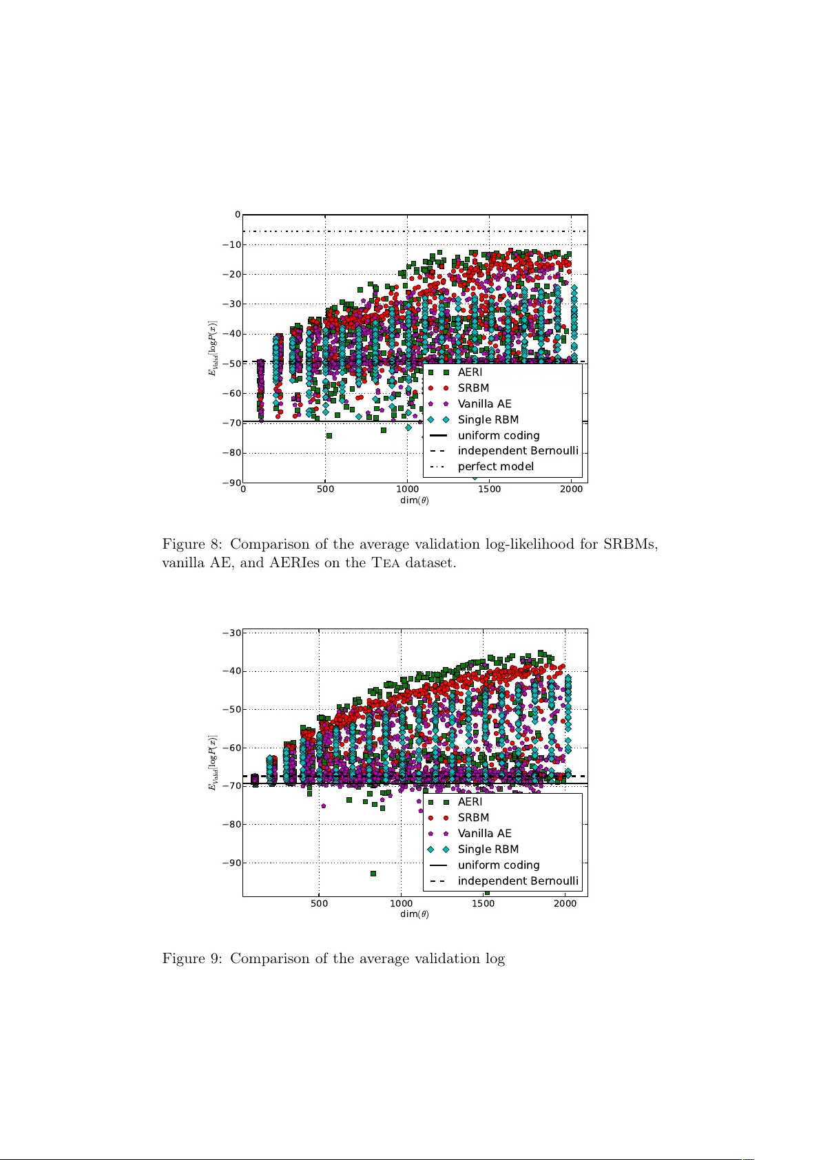
La y er-wise training of deep generativ e mo dels Ludo vic Arnold, Y ann Ollivier Abstract When using deep, multi-la y ered architectures to build generativ e mo dels of data, it is difficult to train all la yers at once. W e propose a lay er-wise training pro cedure admitting a p erformance guarantee compared to the global optimum. It is based on an optimistic proxy of future p erformance, the b est latent mar ginal . W e interpret auto- enco ders in this setting as generativ e mo dels, by showing that they train a low er b ound of this criterion. W e test the new learning pro cedure against a state of the art method (stac ked RBMs), and find it to improv e p erformance. Both theory and exp erimen ts highligh t the imp ortance, when training deep arc hitectures, of using an inference mo del (from data to hidden v ariables) ric her than the generativ e mo del (from hidden v ariables to data). In tro duction Deep architectures, such as m ultiple-lay er neural net works, hav e recently b een the ob ject of a lot of interest and hav e b een sho wn to provide state-of-the-art p erformance on man y problems [ 3 ]. A k ey asp ect of deep learning is to help in learning b etter representations of the data, th us reducing the need for hand-crafted features, a v ery time-consuming pro cess requiring exp ert kno wledge. Due to the difficulty of training a whole deep net w ork at once, a so- called layer-wise pro cedure is used as an approximation [ 12 , 1 ]. How ev er, a long-standing issue is the justification of this lay er-wise training: although the metho d has shown its merits in practice, theoretical justifications fall somewhat short of exp ectations. A frequently cited result [ 12 ] is a pro of that adding la yers increases a so-called v ariational lo wer bound on the log-likelihoo d of the mo del, and therefore that adding la yers c an improv e p erformance. W e reflect on the v alidity of lay er-wise training pro cedures, and discuss in what wa y and with what assumptions they can b e construed as b eing equiv alent to the non-lay er-wise, that is, whole-net work, training. This leads us to a new approach for training deep generative mo dels, using a new criterion for optimizing each lay er starting from the b ottom and for transferring the problem upw ards to the next la yer. Under the righ t conditions, this new 1 la yer-wise approach is equiv alen t to optimizing the log-likelihoo d of the full deep generative mo del (Theorem 1 ). As a first step, in Section 1 we re-introduce the general form of deep generativ e mo dels, and derive the gradient of the log-lik eliho o d for deep mo dels. This gradien t is seldom ev er considered b ecause it is considered in tractable and requires sampling from complex distributions. Hence the need for a simpler, la yer-wise training pro cedure. W e then show (Section 2.1 ) ho w an optimistic criterion, the BLM upp er b ound , can b e used to train optimal low er la yers pro vided subsequent training of upp er lay ers is successful, and discuss what criterion to use to transfer the learning problem to the upp er la yers. This leads to a discussion of the relation of this pro cedure with stac ked restricted Boltzmann machines (SRBMs) and auto-enco ders (Sections 2.3 and 2.4 ), in which a new justification is found for auto-enco ders as optimizing the low er part of a deep generative mo del. In Section 2.7 we sp ell out the theoretical adv an tages of using a mo del for the hidden v ariable h ha ving the form 𝑄 ( h ) = 𝑞 ( h | x ) 𝑃 data ( x ) when lo oking for hidden-v ariable generative mo dels of the data x , a scheme close to that of auto-enco ders. Finally , we discuss new applications and p erform exp erimen ts (Section 3 ) to v alidate the approach and compare it to state-of-the-art metho ds, on tw o new deep datasets, one syn thetic and one real. In particular we introduce auto-enco ders with rich inference (AERIes) whic h are auto-enco ders mo dified according to this framework. Indeed b oth theory and exp erimen ts strongly suggest that, when using stac ked auto-asso ciators or similar deep arc hitectures, the inference part (from data to laten t v ariables) should use a muc h richer model than the generativ e part (from latent v ariables to data), in fact, as rich as p ossible. Using richer inference helps to find muc h b etter parameters for the same giv en generativ e mo del. 1 Deep generativ e mo dels Let us go bac k to the basic form ulation of training a deep arc hitecture as a traditional learning problem: optimizing the parameters of the whole arc hitecture seen as a probabilistic generativ e mo del of the data. 1.1 Deep mo dels: probabilit y decomp osition The goal of generative learning is to estimate the parameters 𝜃 = ( 𝜃 1 , . . . , 𝜃 𝑛 ) of a distribution 𝑃 𝜃 ( x ) in order to appro ximate a data distribution 𝑃 𝒟 ( x ) on some observed v ariable x . The recen t dev elopment of deep architectures [ 12 , 1 ] has giv en imp ortance to a particular case of latent variable mo dels in which the distribution of x 2 can b e decomp osed as a sum o ver states of laten t v ariables h , 𝑃 𝜃 ( x ) =  h 𝑃 𝜃 1 ,...,𝜃 𝑘 ( x | h ) 𝑃 𝜃 𝑘 +1 ,...,𝜃 𝑛 ( h ) with separate parameters for the marginal probability of h and the conditional probabilit y of x giv en h . Setting 𝐼 = { 1 , 2 , . . . , 𝑘 } suc h that 𝜃 𝐼 is the set of parameters of 𝑃 ( x | h ) and 𝐽 = { 𝑘 + 1 , . . . , 𝑛 } suc h that 𝜃 𝐽 is the set of parameters of 𝑃 ( h ) , this rewrites as 𝑃 𝜃 ( x ) =  h 𝑃 𝜃 𝐼 ( x | h ) 𝑃 𝜃 𝐽 ( h ) (1) In deep architectures, the same kind of decomp osition is applied to h itself recursively , thus defining a la yered mo del with several hidden lay ers h (1) , h (2) , . . . , h ( 𝑘 max ) , namely 𝑃 𝜃 ( x ) =  h (1) 𝑃 𝜃 𝐼 0 ( x | h (1) ) 𝑃 𝜃 𝐽 0 ( h (1) ) (2) 𝑃 ( h ( 𝑘 ) ) =  h ( 𝑘 +1) 𝑃 𝜃 𝐼 𝑘 ( h ( 𝑘 ) | h ( 𝑘 +1) ) 𝑃 𝜃 𝐽 𝑘 ( h ( 𝑘 +1) ) , 1 6 𝑘 6 𝑘 max − 1 (3) A t an y one time, w e will only b e inter ested in one step of this decomp osi- tion. Th us for simplicit y , we consider that the distribution of interest is on the observe d v ariable x , with latent v ariable h . The results extend to the other lay ers of the decomp osition by renaming v ariables. In Sections 2.3 and 2.4 we quic kly present t wo frequen tly used deep arc hitectures, stac ked RBMs and auto-enco ders, within this framework. 1.2 Data log-lik eliho o d The goal of the learning pro cedure, for a probabilistic generative mo del, is generally to maximize the log-likelihoo d of the data under the mo del, namely , to find the v alue of the parameter 𝜃 * = ( 𝜃 * 𝐼 , 𝜃 * 𝐽 ) achieving 𝜃 * : = arg max 𝜃 E x ∼ 𝑃 𝒟 [log 𝑃 𝜃 ( x )] (4) = arg min 𝜃 𝐷 KL ( 𝑃 𝒟 ‖ 𝑃 𝜃 ) , (5) where 𝑃 𝒟 is the empirical data distribution, and 𝐷 KL ( · ‖ · ) is the Kullback– Leibler divergence. (F or simplicity we assume this optimum is unique.) An obvious wa y to tackle this problem w ould be a gradient ascent ov er the full parameter 𝜃 . Ho wev er, this is impractical for deep architectures (Section 1.3 b elo w). It would b e easier to b e able to train deep architectures in a lay er-wise fashion, by first training the parameters 𝜃 𝐼 of the b ottom lay er, deriving a 3 new target distribution for the latent v ariables h , and then training 𝜃 𝐽 to repro duce this target distribution on h , recursively ov er the lay ers, till one reac hes the top lay er on which, hop efully , a simple probabilistic generative mo del can b e used. Indeed this is often done in practice, except that the ob jectiv e ( 4 ) is replaced with a surrogate ob jectiv e. F or instance, for architectures made of stac ked RBMs, at eac h level the likelihoo d of a single RBM is maximized, ignoring the fact that it is to b e used as part of a deep architecture, and moreo ver often using a further appro ximation to the lik eliho o d suc h as con trastive div ergence [ 11 ]. Under sp ecific conditions (i.e., initializing the upp er lay er with an upside-down version of the current RBM), it can b e sho wn that adding a lay er improv es a lo wer b ound on p erformance [ 12 ]. W e address in Section 2 the following questions: Is it p ossible to compute or estimate the optimal v alue of the parameters 𝜃 * 𝐼 of the b ottom la yer, without training the whole mo del? Is it p ossible to compare t wo v alues of 𝜃 𝐼 without training the whole mo del? The latter would b e particularly con venien t for hyper-parameter selection, as it w ould allow to compare low er- la yer mo dels b efore the upp er lay ers are trained, thus significantly reducing the size of the h yp er-parameter searc h space from exp onential to linear in the num b er of lay ers. W e prop ose a pro cedure aimed at reac hing the global optim um 𝜃 * in a la yer-wise fashion, based on an optimistic estimate of log-lik eliho o d, the b est latent mar ginal (BLM) upp er b ound . W e study its theoretical guaran tees in Section 2 . In Section 3 we make an exp erimen tal comparison betw een stac ked RBMs, auto-enco ders mo dified according to this sc heme, and v anilla auto-enco ders, on tw o simple but deep datasets. 1.3 Learning b y gradient ascen t for deep arc hitectures Maximizing the lik eliho o d of the data distribution 𝑃 𝒟 ( x ) under a mo del, or equiv alently minimizing the KL-divergence 𝐷 KL ( 𝑃 𝒟 ‖ 𝑃 𝜃 ) , is usually done with gradient ascen t in the parameter space. The deriv ativ e of the log-likelihoo d for a deep generativ e mo del can b e written as: 𝜕 log 𝑃 𝜃 ( x ) 𝜕 𝜃 =  h 𝜕 𝑃 𝜃 𝐼 ( x | h ) 𝜕 𝜃 𝑃 𝜃 𝐽 ( h ) +  h 𝑃 𝜃 𝐼 ( x | h ) 𝜕 𝑃 𝜃 𝐽 ( h ) 𝜕 𝜃 𝑃 𝜃 ( x ) (6) =  h 𝜕 log 𝑃 𝜃 𝐼 ( x | h ) 𝜕 𝜃 𝑃 𝜃 ( h | x ) +  h 𝜕 log 𝑃 𝜃 𝐽 ( h ) 𝜕 𝜃 𝑃 𝜃 ( h | x ) (7) b y rewriting 𝑃 𝜃 ( h ) /𝑃 𝜃 ( x ) = 𝑃 𝜃 ( h | x ) /𝑃 𝜃 ( x | h ) . The deriv ativ e w.r.t. a given comp onen t 𝜃 𝑖 of 𝜃 simplifies b ecause 𝜃 𝑖 is either a parameter of 𝑃 𝜃 𝐼 ( x | h ) 4 when 𝑖 ∈ 𝐼 , or a parameter of 𝑃 𝜃 𝐽 ( h ) when 𝑖 ∈ 𝐽 : ∀ 𝑖 ∈ 𝐼 , 𝜕 log 𝑃 𝜃 ( x ) 𝜕 𝜃 𝑖 =  h 𝜕 log 𝑃 𝜃 𝐼 ( x | h ) 𝜕 𝜃 𝑖 𝑃 𝜃 𝐼 ,𝜃 𝐽 ( h | x ) , (8) ∀ 𝑖 ∈ 𝐽, 𝜕 log 𝑃 𝜃 ( x ) 𝜕 𝜃 𝑖 =  h 𝜕 log 𝑃 𝜃 𝐽 ( h ) 𝜕 𝜃 𝑖 𝑃 𝜃 𝐼 ,𝜃 𝐽 ( h | x ) . (9) Unfortunately , this gradien t ascen t pro cedure is generally intractable, b ecause it requires sampling from 𝑃 𝜃 𝐼 ,𝜃 𝐽 ( h | x ) (where b oth the upp er lay er and lo wer la yer influence h ) to p erform inference in the deep mo del. 2 La y er-wise deep learning 2.1 A theoretical guarantee W e no w presen t a training pro cedure that w orks successively on each la yer. First w e train 𝜃 𝐼 together with a conditional mo del 𝑞 ( h | x ) for the latent v ariable kno wing the data. This step inv olv es only the bottom part of the mo del and is thus often tractable. This allows to infer a new target distribution for h , on whic h the upp er lay ers can then b e trained. This pro cedure singles out a particular setting ˆ 𝜃 𝐼 for the b ottom lay er of a deep architecture, based on an optimistic assumption of what the upp er la yers ma y b e able to do (cf. Prop osition 3 ). Under this pro cedure, Theorem 1 states that it is p ossible to obtain a v alidation that the parameter ˆ 𝜃 𝐼 for the b ottom lay er was optimal, pro vided the rest of the training go es w ell. Namely , if the target distribution for h can b e realized or well approximated by some v alue of the parameters 𝜃 𝐽 of the top lay ers, and if 𝜃 𝐼 w as obtained using a ric h enough conditional mo del 𝑞 ( h | x ) , then ( 𝜃 𝐼 , 𝜃 𝐽 ) is guaran teed to b e globally optimal. Theorem 1. Supp ose the p ar ameters 𝜃 𝐼 of the b ottom layer ar e tr aine d by ( ˆ 𝜃 𝐼 , ˆ 𝑞 ) : = arg max 𝜃 𝐼 ,𝑞 E x ∼ 𝑃 𝒟  log  h 𝑃 𝜃 𝐼 ( x | h ) 𝑞 𝒟 ( h )  (10) wher e the ar g max runs over all c onditional pr ob ability distributions 𝑞 ( h | x ) and wher e 𝑞 𝒟 ( h ) : =  ˜ x 𝑞 ( h | ˜ x ) 𝑃 𝒟 ( ˜ x ) (11) with 𝑃 𝒟 the observe d data distribution. W e c al l the optimal ˆ 𝜃 𝐼 the b est optimistic low er la yer (BOLL). L et ˆ 𝑞 𝒟 ( h ) b e the distribution on h asso ciate d with the optimal ˆ 𝑞 . Then: 5 ∙ If the top layers c an b e tr aine d to r epr o duc e ˆ 𝑞 𝒟 ( h ) p erfe ctly, i.e., if ther e exists a p ar ameter ˆ 𝜃 𝐽 for the top layers such that the distribution 𝑃 ^ 𝜃 𝐽 ( h ) is e qual to ˆ 𝑞 𝒟 ( h ) , then the p ar ameters obtaine d ar e glob al ly optimal: ( ˆ 𝜃 𝐼 , ˆ 𝜃 𝐽 ) = ( 𝜃 * 𝐼 , 𝜃 * 𝐽 ) ∙ Whatever p ar ameter value 𝜃 𝐽 is use d on the top layers in c onjunction with the BOLL ˆ 𝜃 𝐼 , the differ enc e in p erformanc e ( 4 ) b etwe en ( ˆ 𝜃 𝐼 , 𝜃 𝐽 ) and the glob al optimum ( 𝜃 * 𝐼 , 𝜃 * 𝐽 ) is at most the Kul lb ack–L eibler diver genc e 𝐷 KL ( ˆ 𝑞 𝒟 ( h ) ‖ 𝑃 𝜃 𝐽 ( h )) b etwe en ˆ 𝑞 𝒟 ( h ) and 𝑃 𝜃 𝐽 ( h ) . This theorem strongly suggests using ˆ 𝑞 𝒟 ( h ) as the target distribution for the top la yers, i.e., lo oking for the v alue ˆ 𝜃 𝐽 b est appro ximating ˆ 𝑞 𝒟 ( h ) : ˆ 𝜃 𝐽 : = arg min 𝜃 𝐽 𝐷 KL ( ˆ 𝑞 𝒟 ( h ) ‖ 𝑃 𝜃 𝐽 ( h )) = arg max 𝜃 𝐽 E h ∼ ^ 𝑞 𝒟 log 𝑃 𝜃 𝐽 ( h ) (12) whic h thus tak es the same form as the original problem. Then the same sc heme may b e used recursiv ely to train the top la yers. A final fine-tuning phase may b e helpful, see Section 2.6 . Note that when the top lay ers fail to approximate ˆ 𝑞 𝒟 p erfectly , the loss of p erformance dep ends only on the observed difference b et w een ˆ 𝑞 𝒟 and 𝑃 ^ 𝜃 𝐽 , and not on the unknown global optim um ( 𝜃 * 𝐼 , 𝜃 * 𝐽 ) . Bew are that, unfortunately , this b ound relies on p erfe ct lay er-wise training of the b ottom lay er, i.e., on ˆ 𝑞 b eing the optimum of the criterion ( 10 ) optimized ov er all p ossible conditional distributions 𝑞 ; otherwise it is a priori not v alid. In practice the supremum on 𝑞 will alw ays b e tak en o ver a restricted set of conditional distributions 𝑞 ( h | x ) , rather than the set of all p ossible distributions on h for each x . Th us, this theorem is an idealized version of practice (though Remark 4 b elo w mitigates this). This still suggests a clear strategy to separate the deep optimization problem into tw o subproblems to b e solv ed sequen tially: 1. T rain the parameters 𝜃 𝐼 of the b ottom lay er after ( 10 ) , using a mo del 𝑞 ( h | x ) as wide as p ossible, to approximate the BOLL ˆ 𝜃 𝐼 . 2. Infer the corresp onding distribution of h b y ( 11 ) and train the upp er part of the mo del as b est as p ossible to appro ximate this distribution. Then, provided learning is successful in b oth instances, the result is close to optimal. Auto-enco ders can b e shown to implemen t an approximation of this pro cedure, in which only the terms x = ˜ x are kept in ( 10 ) – ( 11 ) (Section 2.4 ). This scheme is designed with in mind a situation in which the upp er la y ers get progessively simpler. Indeed, if the lay er for h is as wide as the la yer for 6 x and if 𝑃 ( x | h ) can learn the identit y , then the pro cedure in Theorem 1 just transfers the problem unchanged one lay er up. This theorem strongly suggests decoupling the inference and generative mo dels 𝑞 ( h | x ) and 𝑃 ( x | h ) , and using a rich conditional mo del 𝑞 ( h | x ) , con- trary , e.g., to common practice in auto-enco ders 1 . Indeed the exp erimen ts of Section 3 confirm that using a more expressiv e 𝑞 ( h | x ) yields impro ved v alues of 𝜃 . Imp ortan tly , 𝑞 ( h | x ) is only used as an auxiliary prop for solving the optimization problem ( 4 ) o ver 𝜃 and is not part of the final generativ e mo del, so that using a ric her 𝑞 ( h | x ) to reac h a b etter v alue of 𝜃 is not simply c hanging to a larger mo del. Th us, using a ric her inference mo del 𝑞 ( h | x ) should not p ose to o muc h risk of ov erfitting b ecause the regularization prop erties of the mo del come mainly from the c hoice of the generativ e mo del family ( 𝜃 ) . The criterion prop osed in ( 10 ) is of particular relev ance to representation learning where the goal is not to learn a generative mo del, but to learn a useful representation of the data. In this setting, training an upper la yer mo del 𝑃 ( h ) b ecomes irrelev ant b ecause we are not interested in the generativ e mo del itself. What matters in representation learning is that the lo wer la yer (i.e., 𝑃 ( x | h ) and 𝑞 ( h | x ) ) is optimal for some mo del of 𝑃 ( h ) , left unsp ecified. W e no w pro ceed, by steps, to the proof of Theorem 1 . This will b e the o ccasion to introduce some concepts used later in the exp erimen tal setting. 2.2 The Best Latent Marginal Upp er Bound One wa y to ev aluate a parameter 𝜃 𝐼 for the b ottom lay er without training the whole architecture is to b e optimistic: assume that the top lay ers will b e able to pro duce the probabilit y distribution for h that gives the b est results if used together with 𝑃 𝜃 𝐼 ( x | h ) . This leads to the following. Definition 2. L et 𝜃 𝐼 b e a value of the b ottom layer p ar ameters. The b est laten t marginal (BLM) for 𝜃 𝐼 is the pr ob ability distribution 𝑄 on h maximizing the lo g-likeliho o d: ˆ 𝑄 𝜃 𝐼 , 𝒟 : = arg max 𝑄 E x ∼ 𝑃 𝒟  log  h 𝑃 𝜃 𝐼 ( x | h ) 𝑄 ( h )  (13) wher e the ar g max runs over the set of al l pr ob ability distributions over h . The BLM upp er b ound is the c orr esp onding lo g-likeliho o d value: 𝒰 𝒟 ( 𝜃 𝐼 ) : = max 𝑄 E x ∼ 𝑃 𝒟  log  h 𝑃 𝜃 𝐼 ( x | h ) 𝑄 ( h )  (14) 1 A ttempts to preven t auto-encoders from learning the iden tity (which is completely justifiable) often result in an ev en more constrained inference mo del, e.g., tied w eights, or sparsit y constraints on the hidden representation. 7 The BLM upp er b ound 𝒰 𝒟 ( 𝜃 𝐼 ) is the least upp er b ound on the log- lik eliho o d of the deep generative mo del on the dataset 𝒟 if 𝜃 𝐼 is used for the b ottom la yer. 𝒰 𝒟 ( 𝜃 𝐼 ) is only an upp er b ound of the actual p erformance of 𝜃 𝐼 , b ecause subsequent training of 𝑃 𝜃 𝐽 ( h ) may b e sub optimal: the b est latent marginal ˆ 𝑄 𝜃 𝐼 , 𝒟 ( h ) may not b e representable as 𝑃 𝜃 𝐽 ( h ) for 𝜃 𝐽 in the mo del, or the training of 𝑃 𝜃 𝐽 ( h ) itself ma y not conv erge to the b est solution. Note that the arg max in ( 13 ) is concav e in 𝑄 , so that in t ypical situations the BLM is unique—except in degenerate cases such as when t wo v alues of h define the same 𝑃 𝜃 𝐼 ( x | h ) ). Prop osition 3. The criterion ( 10 ) use d in The or em 1 for tr aining the b ottom layer c oincides with the BLM upp er b ound: 𝒰 𝒟 ( 𝜃 𝐼 ) = max 𝑞 E x ∼ 𝑃 𝒟  log  h 𝑃 𝜃 𝐼 ( x | h ) 𝑞 𝒟 ( h )  (15) wher e the maximum runs over al l c onditional pr ob ability distributions 𝑞 ( h | x ) . In p articular the BOLL ˆ 𝜃 𝐼 sele cte d in The or em 1 is ˆ 𝜃 𝐼 = arg max 𝜃 𝐼 𝒰 𝒟 ( 𝜃 𝐼 ) (16) and the tar get distribution ˆ 𝑞 𝒟 ( h ) in The or em 1 is the b est latent mar ginal ˆ 𝑄 ^ 𝜃 𝐼 , 𝒟 . Th us the BOLL ˆ 𝜃 𝐼 is the b est b ottom la yer setting if one uses an optimistic criterion for assessing the b ottom lay er, hence the name “b est optimistic low er la yer”. Pr o of. An y distribution 𝑄 o ver h can b e written as 𝑞 𝒟 for some conditional distribution 𝑞 ( h | x ) , for instance by defining 𝑞 ( h | x ) = 𝑄 ( h ) for every x in the dataset. In particular this is the case for the b est laten t marginal ˆ 𝑄 𝜃 𝐼 , 𝒟 . Consequen tly the maxima in ( 15 ) and in ( 14 ) are taken on the same set and coincide. The argument that an y distribution is of the form 𝑞 𝒟 ma y lo ok disapp oin t- ing: why choose this particular form? In Section 2.7 w e sho w ho w writing distributions ov er h as 𝑞 𝒟 for some conditional distribution 𝑞 ( h | x ) may help to maximize data log-lik eliho o d, by quantifiably incorp orating information from the data (Prop osition 7 ). Moreov er, the b ound on loss of p erformance (second part of Theorem 1 ) when the upp er lay ers do not matc h the BLM crucially relies on the prop erties of ˆ 𝑞 𝒟 . A more practical argument for using 𝑞 𝒟 is that optimizing both 𝜃 𝐼 and the full distribution of the hidden v ariable h at the same time is just as difficult as optimizing the whole netw ork, whereas the deep architectures curren tly in use already train a mo del of x kno wing h and of h knowing x at the same time. 8 Remark 4. F or The or em 1 to hold, it is not ne c essary to optimize over al l p ossible c onditional pr ob ability distributions 𝑞 ( h | x ) (which is a set of very lar ge dimension). As c an b e se en fr om the pr o of ab ove it is enough to optimize over a family 𝑞 ( h | x ) ∈ 𝒬 such that every (non-c onditional) distribution on h c an b e r epr esente d (or wel l appr oximate d) as 𝑞 𝒟 ( h ) for some 𝑞 ∈ 𝒬 . Let us no w go on with the pro of of Theorem 1 . Prop osition 5. Set the b ottom layer p ar ameters to the BOLL ˆ 𝜃 𝐼 = arg max 𝜃 𝐼 𝒰 𝒟 ( 𝜃 𝐼 ) (17) and let ˆ 𝑄 b e the c orr esp onding b est latent mar ginal. Assume that subse quent tr aining of the top layers using ˆ 𝑄 as the tar get distribution for h , is suc c essful, i.e., ther e exists a 𝜃 𝐽 such that ˆ 𝑄 ( h ) = 𝑃 𝜃 𝐽 ( h ) . Then ˆ 𝜃 𝐼 = 𝜃 * 𝐼 . Pr o of. Define the in-mo del BLM upp er b ound as 𝒰 model 𝒟 ( 𝜃 𝐼 ) : = max 𝜃 𝐽 E x ∼ 𝑃 𝒟  log  h 𝑃 𝜃 𝐼 ( x | h ) 𝑃 𝜃 𝐽 ( h )  (18) By definition, the global optim um 𝜃 * 𝐼 for the parameters of the whole arc hitecture is given b y 𝜃 * 𝐼 = arg max 𝜃 𝐼 𝒰 model 𝒟 ( 𝜃 𝐼 ) . Ob viously , for any v alue 𝜃 𝐼 w e ha ve 𝒰 model 𝒟 ( 𝜃 𝐼 ) 6 𝒰 𝒟 ( 𝜃 𝐼 ) since the argmax is tak en o ver a more restricted set. Then, in turn, 𝒰 𝒟 ( 𝜃 𝐼 ) 6 𝒰 𝒟 ( ˆ 𝜃 𝐼 ) b y definition of ˆ 𝜃 𝐼 . By our assumption, the BLM ˆ 𝑄 for ˆ 𝜃 𝐼 happ ens to lie in the mo del: ˆ 𝑄 ( h ) = 𝑃 𝜃 𝐽 ( h ) . This implies that 𝒰 𝒟 ( ˆ 𝜃 𝐼 ) = 𝒰 model 𝒟 ( ˆ 𝜃 𝐼 ) . Com bining, we get that 𝒰 model 𝒟 ( 𝜃 𝐼 ) 6 𝒰 model 𝒟 ( ˆ 𝜃 𝐼 ) for any 𝜃 𝐼 . Thus ˆ 𝜃 𝐼 maximizes 𝒰 model 𝒟 ( 𝜃 𝐼 ) , and is thus equal to 𝜃 * 𝐼 . The first part of Theorem 1 then results from the combination of Prop o- sitions 5 and 3 . W e now give a b ound on the loss of p erformance in case further training of the upp er lay ers fails to repro duce the BLM. This will complete the pro of of Theorem 1 . W e will make use of a sp ecial optimality property of distributions of the form 𝑞 𝒟 ( h ) , namely , Proposition 7 , whose proof is p ostponed to Section 2.7 . Prop osition 6. Ke ep the notation of The or em 1 . In the c ase when 𝑃 𝜃 𝐽 ( h ) fails to r epr o duc e ˆ 𝑞 𝒟 ( h ) exactly, the loss of p erformanc e of ( ˆ 𝜃 𝐼 , 𝜃 𝐽 ) with r esp e ct to the glob al optimum ( 𝜃 * 𝐼 , 𝜃 * 𝐽 ) is at most 𝐷 KL ( 𝑃 𝒟 ( x ) ‖ 𝑃 ^ 𝜃 𝐼 ,𝜃 𝐽 ( x )) − 𝐷 KL ( 𝑃 𝒟 ( x ) ‖ ˆ 𝑞 𝒟 , ^ 𝜃 𝐼 ( x )) (19) 9 wher e ˆ 𝑞 𝒟 , ^ 𝜃 𝐼 ( x ) : =  h 𝑃 ^ 𝜃 𝐼 ( x | h ) ˆ 𝑞 𝒟 ( h ) is the distribution on x obtaine d by using the BLM. This quantity is in turn at most 𝐷 KL ( ˆ 𝑞 𝒟 ( h ) ‖ 𝑃 𝜃 𝐽 ( h )) (20) which is thus also a b ound on the loss of p erformanc e of ( ˆ 𝜃 𝐼 , 𝜃 𝐽 ) with r esp e ct to ( 𝜃 * 𝐼 , 𝜃 * 𝐽 ) . Note that these estimates do not dep end on the unk own global optimum 𝜃 * . Imp ortan tly , this b ound is not v alid if ˆ 𝑞 has not b een p erfectly optimized o ver all p ossible conditional distributions 𝑞 ( h | x ) . Thus it should not b e used blindly to get a p erformance b ound, since heuristics will alwa ys b e used to find ˆ 𝑞 . Therefore, it may ha ve only limited practical relev ance. In practice the real loss may b oth b e larger than this b ound b ecause 𝑞 has b een optimized o ver a smaller set, and smaller b ecause we are comparing to the BLM upp er b ound whic h is an optimistic assessment. Pr o of. F rom ( 4 ) and ( 5 ) , the difference in log-lik eliho o d p erformance b et w een an y t wo distributions 𝑝 1 ( x ) and 𝑝 2 ( x ) is equal to 𝐷 KL ( 𝑃 𝒟 ‖ 𝑝 1 ) − 𝐷 KL ( 𝑃 𝒟 ‖ 𝑝 2 ) . F or simplicit y , denote 𝑝 1 ( x ) = 𝑃 ^ 𝜃 𝐼 ,𝜃 𝐽 ( x ) =  h 𝑃 ^ 𝜃 𝐼 ( x | h ) 𝑃 𝜃 𝐽 ( h ) 𝑝 2 ( x ) = 𝑃 𝜃 * 𝐼 ,𝜃 * 𝐽 ( x ) =  h 𝑃 𝜃 * 𝐼 ( x | h ) 𝑃 𝜃 * 𝐽 ( h ) 𝑝 3 ( x ) =  h 𝑃 ^ 𝜃 𝐼 ( x | h ) ˆ 𝑞 𝒟 ( h ) W e w ant to compare 𝑝 1 and 𝑝 2 . Define the in-mo del upp er b ound 𝒰 model 𝒟 ( 𝜃 𝐼 ) as in ( 18 ) ab o v e. Then w e ha ve 𝜃 * 𝐼 = arg max 𝜃 𝐼 𝒰 model 𝒟 ( 𝜃 𝐼 ) and ˆ 𝜃 𝐼 = arg max 𝜃 𝐼 𝒰 𝒟 ( 𝜃 𝐼 ) . Since 𝒰 model 𝒟 6 𝒰 𝒟 , w e hav e 𝒰 model 𝒟 ( 𝜃 * 𝐼 ) 6 𝒰 𝐷 ( ˆ 𝜃 𝐼 ) . The BLM upp er b ound 𝒰 𝐷 ( ˆ 𝜃 𝐼 ) is attained when we use ˆ 𝑞 𝒟 as the distribution for h , so 𝒰 model 𝒟 ( 𝜃 * 𝐼 ) 6 𝒰 𝐷 ( ˆ 𝜃 𝐼 ) means that the p erformance of 𝑝 3 is b etter than the p erformance of 𝑝 2 : 𝐷 KL ( 𝑃 𝒟 ‖ 𝑝 3 ) 6 𝐷 KL ( 𝑃 𝒟 ‖ 𝑝 2 ) (inequalities hold in the rev erse order for data log-likelihoo d). No w by definition of the optimum 𝜃 * , the distribution 𝑝 2 is b etter than 𝑝 1 : 𝐷 KL ( 𝑃 𝒟 ‖ 𝑝 2 ) 6 𝐷 KL ( 𝑃 𝒟 ‖ 𝑝 1 ) . Consequen tly , the difference in p erformance b et w een 𝑝 2 and 𝑝 1 (whether expressed in data log-likelihoo d or in Kullbac k– Leibler divergence) is smaller than the difference in p erformance b et ween 𝑝 3 and 𝑝 1 , which is the difference of Kullbac k–Leibler div ergences app earing in the prop osition. 10 Let us now ev aluate more precisely the loss of 𝑝 1 with respect to 𝑝 3 . By abuse of notation w e will indifferen tly denote 𝑝 1 ( h ) and 𝑝 1 ( x ) , it b eing understo od that one is obtained from the other through 𝑃 ^ 𝜃 𝐼 ( x | h ) , and likewise for 𝑝 3 (with the same ˆ 𝜃 𝐼 ). F or any distributions 𝑝 1 and 𝑝 3 the loss of p erformance of 𝑝 1 w.r.t. 𝑝 3 satisfies E x ∼ 𝑃 𝒟 log 𝑝 3 ( x ) − E x ∼ 𝑃 𝒟 log 𝑝 1 ( x ) = E x ∼ 𝑃 𝒟  log  h 𝑃 ^ 𝜃 𝐼 ( x | h ) 𝑝 3 ( h )  h 𝑃 ^ 𝜃 𝐼 ( x | h ) 𝑝 1 ( h )  and by the log sum inequalit y log (  𝑎 𝑖 /  𝑏 𝑖 ) 6 1  𝑎 𝑖  𝑎 𝑖 log ( 𝑎 𝑖 /𝑏 𝑖 ) [ 9 , Theorem 2.7.1] w e get E x ∼ 𝑃 𝒟 log 𝑝 3 ( x ) − E x ∼ 𝑃 𝒟 log 𝑝 1 ( x ) 6 E x ∼ 𝑃 𝒟  1  h 𝑃 ^ 𝜃 𝐼 ( x | h ) 𝑝 3 ( h )  h 𝑃 ^ 𝜃 𝐼 ( x | h ) 𝑝 3 ( h ) log 𝑃 ^ 𝜃 𝐼 ( x | h ) 𝑝 3 ( h ) 𝑃 ^ 𝜃 𝐼 ( x | h ) 𝑝 1 ( h )  = E x ∼ 𝑃 𝒟  1 𝑝 3 ( x )  h 𝑝 3 ( x , h ) log 𝑝 3 ( h ) 𝑝 1 ( h )  = E x ∼ 𝑃 𝒟   h 𝑝 3 ( h | x ) log 𝑝 3 ( h ) 𝑝 1 ( h )  = E x ∼ 𝑃 𝒟 E h ∼ 𝑝 3 ( h | x )  log 𝑝 3 ( h ) 𝑝 1 ( h )  Giv en a probabilit y 𝑝 3 on ( x , h ) , the law on h obtained by taking an x according to 𝑃 𝒟 , then taking an h according to 𝑝 3 ( h | x ) , is generally not equal to 𝑝 3 ( h ) . How ev er, here 𝑝 3 is equal to the BLM ˆ 𝑞 𝐷 , and b y Prop osition 7 b elow the BLM has exactly this prop ert y (which characterizes the log-likelihoo d extrema). Thus thanks to Prop osition 7 w e ha ve E x ∼ 𝑃 𝒟 E h ∼ ^ 𝑞 𝒟 ( h | x )  log ˆ 𝑞 𝒟 ( h ) 𝑝 1 ( h )  = E h ∼ ^ 𝑞 𝒟  log ˆ 𝑞 𝒟 ( h ) 𝑝 1 ( h )  = 𝐷 KL ( ˆ 𝑞 𝒟 ( h ) ‖ 𝑝 1 ( h )) whic h concludes the argumen t. 2.3 Relation with Stack ed RBMs Stac ked RBMs (SRBMs) [ 12 , 1 , 14 ] are deep generativ e mo dels trained by stac king restricted Boltzmann mac hines (RBMs) [ 23 ]. A RBM uses a single set of parameters to represen t a distribution on pairs ( x , h ) . Similarly to our approac h, stac ked RBMs are trained in a greedy la yer-wise fashion: one starts by training the distribution of the b ottom RBM to approximate the distribution of x . T o do so, distributions 𝑃 𝜃 𝐼 ( x | h ) and 𝑄 𝜃 𝐼 ( h | x ) are learned join tly using a single set of parameters 𝜃 𝐼 . Then a 11 target distribution for h is defined as  x 𝑄 𝜃 𝐼 ( h | x ) 𝑃 𝒟 ( x ) (similarly to ( 11 ) ) and the top lay ers are trained recursively on this distribution. In the final generative mo del, the full top RBM is used on the top lay er to provide a distribution for h , then the b ottom RBMs are used only for the generation of x kno wing h . (Therefore the h -biases of the b ottom RBMs are nev er used in the final generativ e mo del.) Th us, in contrast with our approach, 𝑃 𝜃 𝐼 ( x | h ) and 𝑄 𝜃 𝐼 ( h | x ) are not trained to maximize the least upp er bound of the likelihoo d of the full deep generativ e mo del but are trained to maximize the lik eliho o d of a single RBM. This procedure has b een shown to be equiv alent to maximizing the lik eliho o d of a deep generativ e model with infinitely man y la yers where the w eights are all tied [ 12 ]. The latter can b e interpreted as an assumption on the future v alue of 𝑃 ( h ) , which is unkno wn when learning the first lay er. As suc h, SRBMs mak e a different assumption ab out the future 𝑃 ( h ) than the one made in ( 10 ). With resp ect to this, the comparison of gradient ascents is instructive: the gradient ascent for training the b ottom RBM tak es a form reminiscent of gradien t ascen t of the global generative mo del ( 7 ) but in whic h the dep endency of 𝑃 ( h ) on the upp er la yers 𝜃 𝐽 is ignored, and instead the distribution 𝑃 ( h ) is tied to 𝜃 𝐼 b ecause the RBM uses a single parameter set for b oth. When adding a new lay er on top of a trained RBM, if the initialization is set to an upside do wn v ersion of the current RBM (which can b e seen as “unrolling” one step of Gibbs sampling), the new deep mo del still matches the sp ecial infinite deep generative mo del with tied weigh ts mentio ned ab o v e. Starting training of the upp er lay er from this initialization guarantees that the new lay er can only increase the likelihoo d [ 12 ]. Ho w ever, this result is only known to hold for t wo lay ers; with more la yers, it is only kno wn that adding lay ers increases a b ound on the lik eliho o d [ 12 ]. In our approach, the p ersp ectiv e is different. During the training of low er la yers, w e consider the b est p ossible mo del for the hidden v ariable. Because of errors which are b ound to o ccur in appro ximation and optimization during the training of the mo del for 𝑃 ( h ) , the lik eliho o d asso ciated with an optimal upp er mo del (the BLM upp er b ound) is exp ected to de cr e ase each time w e actually take another lo wer la yer into accoun t: At each new la yer, errors in appro ximation or optimization o ccur so that the final likelihoo d of the training set will b e smaller than the upp er bound. (On the other w a y these limitations migh t actually improv e p erformance on a test set, see the discussion ab out regularization in Section 3 .) In [ 16 ] a training criterion is suggested for SRBMs which is reminiscent of a BLM with tied weigh ts for the inference and generativ e parts (and therefore without the BLM optimality guaran tee), see also Section 2.5 . 12 2.4 Relation with Auto-Enco ders Since the introduction of deep neural netw orks, auto-enco ders [ 24 ] hav e b een considered a credible alternativ e to stack ed RBMs and hav e b een sho wn to ha ve almost identical p erformance on several tasks [ 15 ]. Auto-enco ders are trained by stacking auto-asso ciators [ 7 ] trained with bac kpropagation. Namely: w e start with a three-lay er net work x ↦→ h (1) ↦→ x trained b y backpropagation to repro duce the data; this provides tw o conditional distributions 𝑃 ( h (1) | x ) and 𝑃 ( x | h (1) ) . Then in turn, another auto-asso ciator is trained as a three-lay er netw ork h (1) ↦→ h (2) ↦→ h (1) , to repro duce the distribution 𝑃 ( h (1) | x ) on h (1) , etc. So as in the learning of SRBMs, auto-enco der training is p erformed in a greedy lay er-wise manner, but with a different criterion: the reconstruction error. Note that after the auto-enco der has b een trained, the deep generative mo del is incomplete b ecause it lacks a generativ e mo del for the distribution 𝑃 ( h 𝑘 max ) of the deep est hidden v ariable, which the auto-enco der do es not pro vide 2 . One p ossibilit y is to learn the top la yer with an RBM, which then completes the generativ e mo del. Concerning the theoretical soundness of stac king auto-asso ciators for train- ing deep generative mo dels, it is kno wn that the training of auto-asso ciators is an appro ximation of the training of RBMs in whic h only the largest term of an expansion of the log-lik eliho o d is kept [ 4 ]. In this sense, SRBM and stac ked auto-asso ciator training appro ximate eac h other (see also Section 2.5 ). Our approach gives a new understanding of auto-enco ders as the lo wer part of a deep generativ e model, b ecause they are trained to maximize a lower b ound of ( 10 ), as follo ws. T o fix ideas, let us consider for ( 10 ) a particular class of conditional distributions 𝑞 ( h | x ) commonly used in auto-associators. Namely , let us parametrize 𝑞 as 𝑞 𝜉 with 𝑞 𝜉 ( h | x ) =  𝑗 𝑞 𝜉 ( ℎ 𝑗 | x ) (21) 𝑞 𝜉 ( ℎ 𝑗 | x ) = sigm(  𝑖 𝑥 𝑖 𝑤 𝑖𝑗 + 𝑏 𝑗 ) (22) where the parameter vector is 𝜉 = { W , b } and sigm ( · ) is the sigmoid function. Giv en a conditional distribution 𝑞 ( h | x ) as in Theorem 1 , let us expand the distribution on x obtained from 𝑃 𝜃 𝐼 ( x | h ) and 𝑞 𝒟 ( h ) : 𝑃 ( x ) =  h 𝑃 𝜃 𝐼 ( x | h ) 𝑞 𝒟 ( h ) (23) =  h 𝑃 𝜃 𝐼 ( x | h )  ˜ x 𝑞 ( h | ˜ x ) 𝑃 𝒟 ( ˜ x ) (24) 2 Auto-asso ciators can in fact b e used as v alid generativ e mo dels from which sampling is p ossible [ 20 ] in the setting of manifold learning but this is b ey ond the scope of this article. 13 where as usual 𝑃 𝒟 is the data distribution. Keeping only the terms x = ˜ x in this expression w e see that 𝑃 ( x ) >  h 𝑃 𝜃 𝐼 ( x | h ) 𝑞 ( h | x ) 𝑃 𝒟 ( x ) (25) T aking the sum of likelihoo ds ov er x in the dataset, this corresp onds to the criterion maximized by auto-asso ciators when they are considered from a probabilistic p ersp ectiv e 3 . Since moreov er optimizing ov er 𝑞 as in ( 10 ) is more general than optimizing ov er the particular class 𝑞 𝜉 , we conclude that the criterion optimize d in auto-asso ciators is a lower b ound on the criterion ( 10 ) pr op ose d in The or em 1 . Keeping only x = ˜ x is justified if w e assume that inference is an approxi- mation of the inv erse of the generativ e pro cess 4 , that is, 𝑃 𝜃 𝐼 ( x | h ) 𝑞 ( h | ˜ x ) ≈ 0 as so on as x  = ˜ x . Th us under this assumption, b oth criteria will b e close, so that Theorem 1 provides a justification for auto-encoder training in this case. On the other hand, this assumption can b e strong: it implies that no h can b e shared b et w een different x , so that for instance tw o observ ations cannot come from the same underlying latent v ariable through a random c hoice. Dep ending on the situation this migh t b e unrealistic. Still, using this as a training criterion might p erform well ev en if the assumption is not fully satisfied. Note that w e c hose the form of 𝑞 𝜉 ( h | x ) to matc h that of the usual auto- asso ciator, but of course we could hav e made a different c hoice such as using a m ultilay er net work for 𝑞 𝜉 ( h | x ) or 𝑃 𝜃 𝐼 ( x | h ) . These p ossibilities will b e explored later in this article. 2.5 F rom stac ked RBMs to auto-enco ders: la yer-wise consis- tency W e now show how imp osing a “lay er-wise consistency” constraint on stack ed RBM training leads to the training criterion used in auto-enco ders with tied w eights. Some of the material here already app ears in [ 16 ]. Let us call layer-wise c onsistent a lay er-wise training pro cedure in which eac h la yer determines a v alue 𝜃 𝐼 for its parameters and a target distribution 3 In all fairness, the training of auto-associators by bac kpropagation, in probabilistic terms, consists in the maximization of 𝑃 ( y | x ) 𝑃 𝒟 ( x ) = 𝑜 ( x ) 𝑃 𝒟 ( x ) with y = x [ 8 ], where 𝑜 is the output function of the neural netw ork. In this persp ective, the hidden v ariable h is not considered as a random v ariable but as an intermediate v alue in the form of 𝑃 ( y | x ) . Here, w e introduce h as an in termediate random v ariable as in [ 18 ]. The criterion we wish to maximize is then 𝑃 ( y | x ) 𝑃 𝒟 ( x ) =  h 𝑓 ( y | h ) 𝑔 ( h | x ) 𝑃 𝒟 ( x ) , with y = x . T raining with backpropagation can b e done by sampling h from 𝑔 ( h | x ) instead of using the raw activ ation v alue of 𝑔 ( h | x ) , but in practice we do not sample h as it do es not significantly affect p erformance. 4 whic h is a reasonable assumption if we are to p erform inference in any meaningful sense of the w ord. 14 𝑃 ( h ) for the upp er la yers which are mutually optimal in the follo wing sense: if 𝑃 ( h ) is used a the distribution of the hidden v ariable, then 𝜃 𝐼 is the b ottom parameter v alue maximizing data log-likelihoo d. The BLM training pro cedure is, b y construction, lay er-wise consistent. Let us try to train stack ed RBMs in a la yer-wise consisten t wa y . Given a parameter 𝜃 𝐼 , SRBMs use the hidden v ariable distribution 𝑄 𝒟 ,𝜃 𝐼 ( h ) = E x ∼ 𝑃 𝒟 𝑃 𝜃 𝐼 ( h | x ) (26) as the target for the next la yer, where 𝑃 𝜃 𝐼 ( h | x ) is the RBM distribution of h kno wing x . The v alue 𝜃 𝐼 and this distribution ov er h are mutually optimal for each other if the distribution on x stemming from this distribution on h , giv en b y 𝑃 (1) 𝜃 𝐼 ( x ) = E h ∼ 𝑄 𝒟 ,𝜃 𝐼 ( h ) 𝑃 𝜃 𝐼 ( x | h ) (27) =  h 𝑃 𝜃 𝐼 ( x | h )  ˜ x 𝑃 𝜃 𝐼 ( h | ˜ x ) 𝑃 𝒟 ( ˜ x ) (28) maximizes log-likelihoo d, i.e., 𝜃 𝐼 = arg min 𝐷 KL ( 𝑃 𝒟 ( x ) ‖ 𝑃 (1) 𝜃 𝐼 ( x )) (29) The distribution 𝑃 (1) 𝜃 𝐼 ( x ) is the one obtained from the data after one “forward- bac kward” step of Gibbs sampling x → h → x (cf. [ 16 ]). But 𝑃 (1) 𝜃 𝐼 ( x ) is also equal to the distribution ( 24 ) for an auto-enco der with tied weigh ts. So the lay er-wise consistency criterion for RBMs coincides with tied-w eights auto-enco der training, up to the appro ximation that in practice auto-enco ders retain only the terms x = ˜ x in the ab o ve (Section 2.4 ). On the other hand, stac ked RBM training trains the parameter 𝜃 𝐼 to appro ximate the data distribution by the RBM distribution: 𝜃 RBM 𝐼 = arg min 𝜃 𝐼 𝐷 KL ( 𝑃 𝒟 ( x ) ‖ 𝑃 RBM 𝜃 𝐼 ( x )) (30) where 𝑃 RBM 𝜃 𝐼 is the probability distribution of the RBM with parameter 𝜃 𝐼 , i.e. the probabilit y distribution after an infinite num b er of Gibbs samplings from the data. Th us, stac ked RBM training and tied-w eight auto-enco der training can b e seen as tw o appro ximations to the lay er-wise consistent optimization problem ( 29 ) , one using the full RBM distribution 𝑃 RBM 𝜃 𝐼 instead of 𝑃 (1) 𝜃 𝐼 and the other using x = ˜ x in 𝑃 (1) 𝜃 𝐼 . It is not clear to us to which extent the criteria ( 29 ) using 𝑃 (1) 𝜃 𝐼 and ( 30 ) using 𝑃 RBM 𝜃 𝐼 actually yield different v alues for the optimal 𝜃 𝐼 : although these t wo optimization criteria are different (unless RBM Gibbs sampling conv erges 15 in one step), it migh t b e that the optimal 𝜃 𝐼 is the same (in whic h case SRBM training would b e la yer-wise consisten t), though this seems unlikely . The 𝜃 𝐼 obtained from the la yer-wise consisten t criterion ( 29 ) using 𝑃 (1) 𝜃 𝐼 ( x ) will alwa ys p erform at least as well as standard SRBM training if the upp er la yers matc h the target distribution on h p erfectly—this follows from its very definition. Nonetheless, it is not clear whether lay er-wise consistency is alwa ys a desirable prop ert y . In SRBM training, replacing the RBM distribution o ver h with the one obtained from the data seemingly breaks lay er-wise consistency , but at the same time it alw a ys impr oves data log-likelihoo d (as a consequence of Prop osition 7 b elo w). F or non-lay er-wise consistent training pro cedures, fine-tuning of 𝜃 𝐼 after more la y ers ha ve been trained w ould impro v e performance. Lay er-wise consisten t pro cedures ma y require this as well in case the upp er lay ers do not matc h the target distribution on h (while non-la yer-wise consistent pro cedures w ould require this ev en with p erfect upp er lay er training). 2.6 Relation to fine-tuning When the approach presen ted in Section 2 is used recursiv ely to train deep generativ e mo dels with sev eral la yers using the criterion ( 10 ) , irrecov erable losses may b e incurred at each step: first, b ecause the optimization problem ( 10 ) ma y b e imp erfectly solv ed, and, second, b ecause eac h la yer w as trained using a BLM assumption ab out what upp er la y ers are able to do, and subsequen t upp er lay er training ma y not match the BLM. Consequently the parameters used for each la yer ma y not b e optimal with resp ect to eac h other. This suggests using a fine-tuning pro cedure. In the case of auto-enco ders, fine-tuning can b e done by backpropagation on all (inference and generativ e) lay ers at once (Figure 1 ). This has b een sho wn to improv e p erformance 5 in several contexts [ 14 , 13 ], which confirms the exp ected gain in p erformance from reco vering earlier approximation losses. In principle, there is no limit to the num ber of lay ers of an auto-enco der that could b e trained at once b y bac kpropagation, but in practice training many la yers at once results in a difficult optimization problem with man y lo cal minima. Lay er-wise training can b e seen as a w ay of dealing with the issue of lo cal minima, providing a solution close to a goo d optimum. This optimum is then reac hed b y global fine-tuning. Fine-tuning can b e described in the BLM framew ork as follows: fine- tuning is the maximization of the BLM upp er b ound ( 10 ) where all the lay ers are considered as one single complex lay er (Figure 1 ). In the case of auto- enco ders, the appro ximation x = ˜ x in ( 10 ) – ( 11 ) is used to help optimization, as explained ab o v e. 5 The exact likelihoo d not b eing tractable for larger mo dels, it is necessary to rely on a pro xy such as classification performance to ev aluate the p erformance of the deep net work. 16 Layer-wise deep learn ing for several l ayers Fine-tunin g of all generative and inf erence layers Figure 1: Deep training with fine-tuning. Note that there is no reason to limit fine-tuning to the end of the lay er- wise pro cedure: fine-tuning may b e used at in termediate stages where any n umber of lay ers hav e b een trained. This fine-tuning procedure w as not applied in the exp erimen ts b elow b ecause our exp erimen ts only hav e one la yer for the b ottom part of the mo del. As mentioned b efore, a generative mo del for the topmost hidden la yer (e.g., an RBM) still needs to b e trained to get a complete generative mo del after fine-tuning. 2.7 Data Incorp oration: Prop erties of 𝑞 𝒟 It is not clear wh y it should b e more interesting to w ork with the conditional distribution 𝑞 ( h | x ) and then define a distribution on h through 𝑞 𝒟 , rather than working directly with a distribution 𝑄 on h . The first answer is practical: optimizing on 𝑃 𝜃 𝐼 ( x | h ) and on the distribu- tion of h sim ultaneously is just the same as optimizing o ver the global net work, while on the other hand the currently used deep architectures pro vide b oth x | h and h | x at the same time. A second answer is mathematical: 𝑞 𝒟 is defined through the dataset 𝒟 . Thus b y w orking on 𝑞 ( h | x ) we can concen trate on the corresp ondence b et w een h and x and not on the full distribution of either, and hop efully this corresp ondence is easier to describ e. Then w e use the dataset 𝒟 to provide 𝑞 𝒟 : so rather than directly crafting a distribution 𝑄 ( h ) , we use a distribution whic h automatically incorp orates asp ects of the data distribution 𝒟 ev en for v ery simple 𝑞 . Hop efully this is b etter; we no w formalize this argumen t. Let us fix the b ottom lay er parameters 𝜃 𝐼 , and consider the problem of finding the b est latent marginal o ver h , i.e., the 𝑄 maximizing the data 17 log-lik eliho o d arg max 𝑄 E x ∼ 𝑃 𝒟  log  h 𝑃 𝜃 𝐼 ( x | h ) 𝑄 ( h )  (31) Let 𝑄 ( h ) b e a candidate distribution. W e might build a b etter one by “reflecting the data” in it. Namely , 𝑄 ( h ) defines a distribution 𝑃 𝜃 𝐼 ( x | h ) 𝑄 ( h ) on ( x , h ) . This distribution, in turn, defines a conditional distribution of h kno wing x in the standard w ay: 𝑄 cond ( h | x ) : = 𝑃 𝜃 𝐼 ( x | h ) 𝑄 ( h )  h ′ 𝑃 𝜃 𝐼 ( x | h ′ ) 𝑄 ( h ′ ) (32) W e can turn 𝑄 cond ( h | x ) into a new distribution on h b y using the data distribution: 𝑄 cond 𝒟 ( h ) : =  x 𝑄 cond ( h | x ) 𝑃 𝒟 ( x ) (33) and in general 𝑄 cond 𝒟 ( h ) will not coincide with the original distribution 𝑄 ( h ) , if only b ecause the definition of the former inv olv es the data whereas 𝑄 is arbitrary . W e will show that this op eration is alwa ys an improv emen t: 𝑄 cond 𝒟 ( h ) alwa ys yields a b etter data log-lik eliho o d than 𝑄 . Prop osition 7. L et data incorp oration b e the map sending a distribution 𝑄 ( h ) to 𝑄 cond 𝒟 ( h ) define d by ( 32 ) and ( 33 ) , wher e 𝜃 𝐼 is fixe d. It has the fol lowing pr op erties: ∙ Data inc orp or ation always incr e ases the data lo g-likeliho o d ( 31 ) . ∙ The b est latent mar ginal ˆ 𝑄 𝜃 𝐼 , 𝒟 is a fixe d p oint of this tr ansformation. Mor e pr e cisely, the distributions 𝑄 that ar e fixe d p oints of data inc orp o- r ation ar e exactly the critic al p oints of the data lo g-likeliho o d ( 31 ) (by c onc avity of ( 31 ) these critic al p oints ar e al l maxima with the same value). In p articular if the BLM is uniquely define d (the ar g max in ( 13 ) is unique), then it is the only fixe d p oint of data inc orp or ation. ∙ Data inc orp or ation 𝑄 ↦→ 𝑄 cond 𝒟 c oincides with one step of the exp e ctation- maximization (EM) algorithm to maximize data lo g-likeliho o d by opti- mizing over 𝑄 for a fixe d 𝜃 𝐼 , with h as the hidden variable. This can b e seen as a justification for constructing the hidden v ariable mo del 𝑄 through an inference mo del 𝑞 ( h | x ) from the data, which is the basic approac h of auto-enco ders and the BLM. Pr o of. Let us first prov e the statement ab out exp ectation-maximization. Since the EM algorithm is kno wn to increase data log-lik eliho o d at each step [ 10 , 25 ], this will pro ve the first statemen t as well. F or simplicity let us assume that the data distribution is uniform ov er the dataset 𝒟 = ( x 1 , . . . , x 𝑛 ) . (Arbitrary data weigh ts can b e appro ximated 18 b y putting the same observ ation several times into the data.) The hidden v ariable of the EM algorithm will b e h , and the parameter ov er whic h the EM optimizes will b e the distribution 𝑄 ( h ) itself. In particular w e k eep 𝜃 𝐼 fixed. The distributions 𝑄 and 𝑃 𝜃 𝐼 define a distribution 𝑃 ( x , h ) : = 𝑃 𝜃 𝐼 ( x | h ) 𝑄 ( h ) o ver pairs ( x , h ) . This extends to a distribution ov er 𝑛 -tuples of observ ations: 𝑃 (( x 1 , h 1 ) , . . . , ( x 𝑛 , h 𝑛 )) =  𝑖 𝑃 𝜃 𝐼 ( x 𝑖 | h 𝑖 ) 𝑄 ( h 𝑖 ) and by summing ov er the states of the hidden v ariables 𝑃 ( x 1 , . . . , x 𝑛 ) =  ( h 1 ,..., h 𝑛 ) 𝑃 (( x 1 , h 1 ) , . . . , ( x 𝑛 , h 𝑛 )) Denote  x = ( x 1 , . . . , x 𝑛 ) and  h = ( h 1 , . . . , h 𝑛 ) . One step of the EM algorithm op erating with the distribution 𝑄 as parameter, is defined as transforming the curren t distribution 𝑄 𝑡 in to the new distribution 𝑄 𝑡 +1 = arg max 𝑄   h 𝑃 𝑡 (  h |  x ) log 𝑃 (  x ,  h ) where 𝑃 𝑡 (  x ,  h ) = 𝑃 𝜃 𝐼 (  x |  h ) 𝑄 𝑡 (  h ) is the distribution obtained by using 𝑄 𝑡 for h , and 𝑃 the one obtained from the distribution 𝑄 o ver which w e optimize. Let us follow a standard argumen t for EM algorithms on 𝑛 -tuples of indep enden t observ ations:   h 𝑃 𝑡 (  h |  x ) log 𝑃 (  x ,  h ) =   h 𝑃 𝑡 (  h |  x ) log  𝑖 𝑃 ( x 𝑖 , h 𝑖 ) =  𝑖   h 𝑃 𝑡 (  h |  x ) log 𝑃 ( x 𝑖 , h 𝑖 ) Since observ ations are indep enden t, 𝑃 𝑡 (  h |  x ) decomp oses as a pro duct and so  𝑖   h (log 𝑃 ( x 𝑖 , h 𝑖 )) 𝑃 𝑡 (  h |  x ) =  𝑖  h 1 ,..., h 𝑛 (log 𝑃 ( x 𝑖 , h 𝑖 ))  𝑗 𝑃 𝑡 ( h 𝑗 | x 𝑗 ) =  𝑖  h 𝑖 (log 𝑃 ( x 𝑖 , h 𝑖 )) 𝑃 𝑡 ( h 𝑖 | x 𝑖 )  𝑗  = 𝑖  h 𝑗 𝑃 𝑡 ( h 𝑗 | x 𝑗 ) but of course  h 𝑗 𝑃 𝑡 ( h 𝑗 | x 𝑗 ) = 1 so that finally   h 𝑃 𝑡 (  h |  x ) log 𝑃 (  x ,  h ) =  𝑖  h 𝑖 (log 𝑃 ( x 𝑖 , h 𝑖 )) 𝑃 𝑡 ( h 𝑖 | x 𝑖 ) =  h  𝑖 (log 𝑃 ( x 𝑖 , h )) 𝑃 𝑡 ( h | x 𝑖 ) =  h  𝑖 (log 𝑃 𝜃 𝐼 ( x 𝑖 | h ) + log 𝑄 ( h )) 𝑃 𝑡 ( h | x 𝑖 ) 19 b ecause 𝑃 ( x , h ) = 𝑃 𝜃 𝐼 ( x | h ) 𝑄 ( h ) . W e hav e to maximize this quantit y o ver 𝑄 . The first term do es not dep end on 𝑄 so we only ha ve to maximize  h  𝑖 (log 𝑄 ( h )) 𝑃 𝑡 ( h | x 𝑖 ) . This latter quan tit y is concav e in 𝑄 , so to find the maximum it is sufficient to exhibit a p oint where the deriv ativ e w.r.t. 𝑄 (sub ject to the constraint that 𝑄 is a probabilit y distribution) v anishes. Let us compute this deriv ativ e. If w e replace 𝑄 with 𝑄 + 𝛿 𝑄 where 𝛿 𝑄 is infinitesimal, the v ariation of the quantit y to b e maximized is  h  𝑖 ( 𝛿 log 𝑄 ( h )) 𝑃 𝑡 ( h | x 𝑖 ) =  h 𝛿 𝑄 ( h ) 𝑄 ( h )  𝑖 𝑃 𝑡 ( h | x 𝑖 ) Let us take 𝑄 = ( 𝑄 𝑡 ) cond 𝒟 . Since we assumed for simplicit y that the data distribution 𝒟 is uniform o ver the sample this ( 𝑄 𝑡 ) cond 𝒟 is 𝑄 ( h ) = ( 𝑄 𝑡 ) cond 𝒟 ( h ) = 1 𝑛  𝑖 𝑃 𝑡 ( h | x 𝑖 ) so that the v ariation of the quantit y to b e maximized is  h 𝛿 𝑄 ( h ) 𝑄 ( h )  𝑖 𝑃 𝑡 ( h | x 𝑖 ) = 𝑛  h 𝛿 𝑄 ( h ) But since 𝑄 and 𝑄 + 𝛿 𝑄 are b oth probability distributions, b oth sum to 1 o ver h so that  h 𝛿 𝑄 ( h ) = 0 . This prov es that this c hoice of 𝑄 is an extrem um of the quan tity to b e maximized. This pro ves the last statemen t of the prop osition. As men tioned ab ov e, it implies the first by the general prop erties of EM. Once the first statement is pro ven, the best latent marginal ˆ 𝑄 𝜃 𝐼 , 𝒟 has to be a fixed p oin t of data incorp oration, b ecause otherwise w e w ould get an even b etter distribution th us con tradicting the definition of the BLM. The only p oin t left to prov e is the equiv alence b et w een critical p oin ts of the log-likelihoo d and fixed p oints of 𝑄 ↦→ 𝑄 cond 𝒟 . This is a simple instance of maximization under constrain ts, as follows. Critical p oints of the data log- lik eliho o d are those for whic h the log-lik eliho o d do es not c hange at first order when 𝑄 is replaced with 𝑄 + 𝛿 𝑄 for small 𝛿 𝑄 . The only constraint on 𝛿 𝑄 is that 𝑄 + 𝛿 𝑄 m ust still b e a probabilit y distribution, so that  h 𝛿 𝑄 ( h ) = 0 b ecause b oth 𝑄 and 𝑄 + 𝛿 𝑄 sum to 1 . 20 The first-order v ariation of log-likelihoo d is 𝛿  𝑖 log 𝑃 ( x 𝑖 ) = 𝛿  𝑖 log   h 𝑃 𝜃 𝐼 ( x 𝑖 | h ) 𝑄 ( h )  =  𝑖 𝛿  h 𝑃 𝜃 𝐼 ( x 𝑖 | h ) 𝑄 ( h )  h 𝑃 𝜃 𝐼 ( x 𝑖 , h ) 𝑄 ( h ) =  𝑖  h 𝑃 𝜃 𝐼 ( x 𝑖 | h ) 𝛿 𝑄 ( h ) 𝑃 ( x 𝑖 ) =  h 𝛿 𝑄 ( h )  𝑖 𝑃 𝜃 𝐼 ( x 𝑖 | h ) 𝑃 ( x 𝑖 ) =  h 𝛿 𝑄 ( h )  𝑖 𝑃 ( x 𝑖 , h ) /𝑄 ( h ) 𝑃 ( x 𝑖 ) =  h 𝛿 𝑄 ( h )  𝑖 𝑃 ( h | x 𝑖 ) 𝑄 ( h ) This must v anish for any 𝛿 𝑄 suc h that  h 𝛿 𝑄 ( h ) = 0 . By elemen tary linear algebra (or Lagrange m ultipliers) this o ccurs if and only if  𝑖 𝑃 ( h | x 𝑖 ) 𝑄 ( h ) do es not dep end on h , i.e., if and only if 𝑄 satisfies 𝑄 ( h ) = 𝐶  𝑖 𝑃 ( h | x 𝑖 ) . Since 𝑄 sums to 1 one finds 𝐶 = 1 𝑛 . Since all along 𝑃 is the probabilit y distribution on x and h defined by 𝑄 and 𝑃 𝜃 𝐼 ( x | h ) , namely , 𝑃 ( x , h ) = 𝑃 𝜃 𝐼 ( x | h ) 𝑄 ( h ) , b y definition w e hav e 𝑃 ( h | x ) = 𝑄 cond ( h | x ) so that the condition 𝑄 ( h ) = 1 𝑛  𝑖 𝑃 ( h | x 𝑖 ) exactly means that 𝑄 = 𝑄 cond 𝒟 , hence the equiv alence b et ween critical p oin ts of log-likelihoo d and fixed p oin ts of data incorp oration. 3 Applications and Exp erimen ts Giv en the approach describ ed ab ov e, we now consider several applications for which w e ev aluate the metho d empirically . The intractabilit y of the log-likelihoo d for deep netw orks mak es direct comparison of sev eral metho ds difficult in general. Often the ev aluation is done by using laten t v ariables as features for a classification task and b y direct visual comparison of samples generated by the mo del [ 14 , 21 ]. Instead, w e introduce t wo new datasets whic h are simple enough for the true log- lik eliho o d to be computed explicitly , yet complex enough to b e relev ant to deep learning. W e first chec k that these tw o datasets are indeed deep. Then we try to assess the impact of the v arious approximations from theory to practice, on the v alidit y of the approac h. W e then apply our metho d to the training of deep b elief netw orks using prop erly mo dified auto-enco ders, and show that the metho d outperforms curren t state of the art. 21 W e also explore the use of the BLM upp er b ound to p erform lay er-wise h yp er-parameter selection and show that it gives an accurate prediction of the future log-lik eliho o d of mo dels. 3.1 Lo w-Dimensional Deep Datasets W e no w introduce t wo new deep datasets of lo w dimension. In order for those datasets to give a reasonable picture of what happ ens in the general case, w e first hav e to make sure that they are relev an t to deep learning, using the follo wing approac h: 1. In the spirit of [ 6 ], we train 1000 RBMs using CD-1 [ 11 ] on the dataset 𝒟 , and ev aluate the log-likelihoo d of a disjoint v alidation dataset 𝒱 under each mo del. 2. W e train 1000 2-lay er deep netw orks using stac ked RBMs trained with CD-1 on 𝒟 , and ev aluate the log-lik eliho o d of 𝒱 under eac h mo del. 3. W e compare the p erformance of each mo del at equal n umber of param- eters. 4. If deep net w orks consisten tly outp erform single RBMs for the same n umber of parameters, the dataset is considered to b e deep. The comparison at equal num b er of parameters is justified by one of the main h yp otheses of deep learning, namely that deep archi tectures are capable of represen ting some functions more compactly than shallow architectures [ 2 ]. Hyp er-parameters tak en into account for h yp er-parameter random searc h are the hidden la yers sizes, CD learning rate and num b er of CD ep o c hs. The corresp onding priors are giv en in T able 1 . In order not to give an obvious head start to deep netw orks, the p ossible lay er sizes are c hosen so that the maxim um n umber of parameters for the single RBM and the deep netw ork are as close as p ossible. Cmnist dataset The Cmnist dataset is a low-dimensional v ariation on the Mnist dataset [ 17 ], containing 12,000 samples of dimension 100. The full dataset is split in to training, v alidation and test sets of 4,000 samples each. The dataset is obtained by taking a 10 × 10 image at the center of eac h Mnist sample and using the v alues in [0,1] as probabilities. The first 10 samples of the Cmnist dataset are sho wn in Figure 2 . W e prop ose t wo baselines to which to compare the log-likelihoo d v alues of mo dels trained on the Cmnist dataset: 1. The uniform co ding sc heme: a mo del which giv es equal probability to all p ossible binary 10 × 10 images. The log-likelihoo d of eac h sample is then − 100 bits, or − 69 . 31 nats. 22 P arameter Prior RBM hidden la yer size 1 to 19 Deep Net hidden lay er 1 size 1 to 16 Deep Net hidden lay er 2 size 1 to 16 inference hidden la yer size 1 to 500 CD learn rate log 𝑈 (10 − 5 , 5 × 10 − 2 ) BP learn rate log 𝑈 (10 − 5 , 5 × 10 − 2 ) CD ep o c hs 20 × (10000 / 𝑁 ) BP ep o c hs 20 × (10000 / 𝑁 ) ANN init 𝜎 𝑈 (0 , 1) T able 1: Search space for hyper-parameters when using random search for a dataset of size 𝑁 . Figure 2: First 10 samples of the Cmnist dataset. 2. The independent Bernoulli mo del in which each pixel is giv en an indep enden t Bernoulli probability . The mo del is trained on the training set. The log-likelihoo d of the v alidation set is − 67 . 38 nats p er sample. The comparison of the log-lik eliho o d of stack ed RBMs with that of single RBMs is presented in Figure 3 and confirms that the Cmnist dataset is deep. Tea dataset The Tea dataset is based on the idea of learning an in v ariance for the amoun t of liquid in several cont ainers: a teap ot and 5 teacups. It con tains 243 distinct samples which are then distributed in to a training, v alidation and test set of 81 samples each. The dataset consists of 10 × 10 images in which the left part of the image represents a (stylized) teap ot of size 10 × 5 . The righ t part of the image represents 5 teacups of size 2 × 5 . The liquid is represented by ones and alwa ys lies at the b ottom of each con tainer. The total amoun t of liquid is alwa ys equal to the capacit y of the teap ot, i.e., there are alwa ys 50 ones and 50 zeros in any given sample. The first 10 samples of the Tea dataset are sho wn in Figure 4 . In order to b etter interpret the log-lik eliho o d of mo dels trained on the Tea dataset, w e prop ose 3 baselines: 1. The uniform co ding scheme: the baseline is the same as for the Cmnist 23 5 0 0 1 0 0 0 1 5 0 0 2 0 0 0 d i m ( θ ) − 7 0 − 6 5 − 6 0 − 5 5 − 5 0 − 4 5 − 4 0 E Va l i d [ l og P ( x ) ] 2 s t a g e s d e e p n e t w o r k S i n g l e R B M u n i f o r m c o d i n g i n d e p e n d e n t B e r n o u l l i Figure 3: Checking that Cmnist is deep: log-likelihoo d of the v alidation dataset 𝒱 under RBMs and SRBM deep det works selected b y h yp er-parameter random search, as a function of the num b er of parameters dim( 𝜃 ) . Figure 4: First 10 samples of the Tea dataset. dataset: − 69 . 31 nats. 2. The indep endent Bernoulli mo del, adjusted on the training set. The log-lik eliho o d of the v alidation set is − 49 . 27 nats p er sample. 3. The p erfect mo del in whic h all 243 samples of the full dataset (consituted b y concatenation of the training, v alidation and test sets) are given the probability 1 243 . The exp ected log-likelihoo d of a sample from the v alidation dataset is then log ( 1 243 ) = − 5 . 49 nats. The comparison of the log-lik eliho o d of stac ked RBMs and single RBMs is presen ted in Figure 5 and confirms that the Tea dataset is deep. 24 0 5 0 0 1 0 0 0 1 5 0 0 2 0 0 0 d i m ( θ ) − 9 0 − 8 0 − 7 0 − 6 0 − 5 0 − 4 0 − 3 0 − 2 0 − 1 0 0 E Va l i d [ l og P ( x ) ] 2 s t a g e s d e e p n e t w o r k S i n g l e R B M u n i f o r m c o d i n g i n d e p e n d e n t B e r n o u l l i p e r f e c t m o d e l Figure 5: Chec king that Tea is deep: log-likelihoo d of the v alidation dataset 𝒱 under RBMs and SRBM deep netw orks selected by hyper-parameter random searc h, as a function of the num b er of parameters dim( 𝜃 ) . 3.2 Deep Generativ e Auto-Enco der T raining A first application of our approach is the training of a deep gener ative mo del using auto-asso ciators. T o this end, we prop ose to train low er la yers using auto-asso ciators and to use an RBM for the generative top lay er mo del. W e will compare three kinds of deep architectures: standard auto-enco ders with an RBM on top (v anilla AEs), the new auto-enc o ders with rich infer enc e (AERIes) suggested by our framework, also with an RBM on top, and, for comparison, stac k ed restricted Boltzmann mac hines (SRBMs). All the mo dels used in this study use the same final generativ e mo del class for 𝑃 ( x | h ) so that the comparison fo cuses on the training pro cedure, on equal ground. SRBMs are considered the state of the art [ 12 , 1 ]—although p erformance can b e increased using ric her mo dels [ 3 ], our fo cus here is not on the mo del but on the la yer-wise training pro cedure for a given mo del class. In ideal circumstances, we would hav e compared the log-likelihoo d ob- tained for each training algorithm with the optim um of a deep learning pro cedure suc h as the full gradient ascent pro cedure (Section 2 ). Instead, since this ideal deep learning pro cedure is intractable, SRBMs serv e as a reference. The new AERIes are auto-enco ders mo dified after the following remark: the complexity of the inference mo del used for 𝑞 ( h | x ) can b e increased safely 25 without risking o verfit and loss of generalization p o wer, b ecause 𝑞 is not part of the final generativ e model, and is used only as a to ol for optimization of the generativ e model parameters. This would suggest that the complexit y of 𝑞 could b e greatly increased with only p ositiv e consequences on the p erformance of the mo del. AERIes exploit this p ossibilit y by ha ving, in eac h la yer, a mo dified auto- asso ciator with tw o hidden la yers instead of one: x → h ′ → h → x . The generativ e part 𝑃 𝜃 𝐼 ( x | h ) will be equiv alen t to that of a regular auto-asso ciator, but the inference part 𝑞 ( h | x ) will hav e greater represen tational pow er because it includes the hidden la yer h ′ (see Figure 7 ). W e will also use the more usual auto-enco ders comp osed of auto-asso ciators with one hidden lay er and tied w eights, commonly encountered in the litera- ture (v anilla AE). F or all mo dels, the deep arc hitecture will b e of depth 2 . The stack ed RBMs will b e made of t wo ordinary RBMs. F or AERIes and v anilla AEs, the lo wer part is made of a single auto-asso ciator (mo dified for AERies), and the generativ e top part is an RBM. (Thus they ha ve one la yer less than depicted for the sake of generalit y in Figures 6 and 7 .) F or AERIes and v anilla AEs the lo wer part of the mo del is trained using the usual bac kpropagation algorithm with cross-entrop y loss, which p erforms gradient ascent for the probability of ( 25 ). The top RBM is then trained to maximize ( 12 ). The comp etitiv eness of eac h mo del will b e ev aluated through a compar- ison in log-likelihoo d o v er a v alidation set distinct from the training set. Comparisons are made for a giv en iden tical n umber of parameters of the generativ e mo del 6 . Eac h mo del will b e given equal c hance to find a go od optim um in terms of the n umber of ev aluations in a hyper-parameter selection pro cedure b y random search. When implementing the training pro cedure prop osed in Section 2 , several appro ximations are needed. An important one, compared to Theorem 1 , is that the distribution 𝑞 ( h | x ) will not really b e trained ov er all p ossible conditional distributions for h kno wing x . Next, training of the upp er lay ers will of course fail to repro duce the BLM p erfectly . Moreo ver, auto-asso ciators use an x = ˜ x appro ximation, cf. ( 25 ) . W e will study the effect of these appro ximations. Let us no w pro vide more details for each mo del. Stac ke d RBMs. F or our comparisons, 1000 stack ed RBMs were trained us- ing the pro cedure from [ 12 ]. W e used random searc h on the h yp er-parameters, whic h are: the sizes of the hidden lay ers, the CD learning rate, and the nu mber of CD ep ochs. 6 Because w e only consider the generative models obtained, 𝑞 is nev er taken in to account in the n umber of parameters of an auto-encoder or SRBM. Ho wev er, the parameters of the top RBM are tak en into account as they are a necessary part of the generative mo del. 26 q(h (1) |x) P(x| h (1) ) input x label x train 1 st layer AA Figure 6: Deep generative auto-enco der training sc heme. V anilla auto-enco ders. The general training algorithm for v anilla auto- enco ders is depicted in Figure 6 . First an auto-asso ciator is trained to maximize the adaptation of the BLM upp er b ound for auto-associators presen ted in ( 25 ) . The maximization procedure itself is done with the bac kpropagation algorithm and cross-entrop y loss. The inference w eights are tied to the generative weigh ts so that W gen = W ⊤ inf as is often the case in practice. An ordinary RBM is used as a generative mo del on the top lay er. 1000 deep generative auto-enco ders were trained using random searc h on the hyper-parameters. Because deep generative auto-enco ders use an RBM as the top lay er, they use the same h yp er-parameters as stac ked RBMs, but also bac kpropagation (BP) learning rate, BP ep o c hs, and ANN init 𝜎 (i.e. the standard deviation of the gaussian used during initialization). Auto-Enco ders with Ric h Inference (AERIes). The mo del and train- ing scheme for AERIes are represen ted in Figure 7 . Just as for v anilla auto-enco ders, w e use the backpro pagation algorithm and cross-entrop y loss to maximize the auto-enco der version ( 25 ) of the BLM upp er b ound on the training set. No w eights are tied, of course, as this do es not make sense for an auto-asso ciator with differen t mo dels for 𝑃 ( x | h ) and 𝑞 ( h | x ) . The top 27 Figure 7: Deep generative mo dified auto-enco der (AERI) training scheme. RBM is trained afterw ards. Hyp er-parameters are the same as ab o v e, with in addition the size of the new hidden la yer h ′ . Results The results of the ab o v e comparisons on the Tea and Cmnist validation datasets are giv en in Figures 8 and 9 . F or b etter readability , the Pareto fron t 7 for each mo del is given in Figures 10 and 11 . As exp ected, all mo dels p erform b etter than the baseline indep enden t Bernoulli mo del but hav e a lo wer likelihoo d than the p erfect mo del 8 . Also, 7 The Pareto front is comp osed of all models which are not subsumed by other models according to the num b er of parameters and the exp ected log-likelihoo d. A mo del is said to b e subsumed b y another if it has strictly more parameters and a w orse likelihoo d. 8 Note that some instances are outp erformed by the uniform co ding scheme, whic h may 28 0 5 0 0 1 0 0 0 1 5 0 0 2 0 0 0 d i m ( θ ) − 9 0 − 8 0 − 7 0 − 6 0 − 5 0 − 4 0 − 3 0 − 2 0 − 1 0 0 E Va l i d [ l og P ( x ) ] A E R I S R B M V a n i l l a A E S i n g l e R B M u n i f o r m c o d i n g i n d e p e n d e n t B e r n o u l l i p e r f e c t m o d e l Figure 8: Comparison of the av erage v alidation log-likelihoo d for SRBMs, v anilla AE, and AERIes on the Tea dataset. 5 0 0 1 0 0 0 1 5 0 0 2 0 0 0 d i m ( θ ) − 9 0 − 8 0 − 7 0 − 6 0 − 5 0 − 4 0 − 3 0 E Va l i d [ l og P ( x ) ] A E R I S R B M V a n i l l a A E S i n g l e R B M u n i f o r m c o d i n g i n d e p e n d e n t B e r n o u l l i Figure 9: Comparison of the av erage v alidation log-likelihoo d for SRBMs, v anilla AE, and AERIes on the Cmnist dataset. 29 0 5 0 0 1 0 0 0 1 5 0 0 2 0 0 0 d i m ( θ ) − 9 0 − 8 0 − 7 0 − 6 0 − 5 0 − 4 0 − 3 0 − 2 0 − 1 0 0 E Va l i d [ l og P ( x ) ] A E R I S R B M V a n i l l a A E S i n g l e R B M u n i f o r m c o d i n g i n d e p e n d e n t B e r n o u l l i p e r f e c t m o d e l Figure 10: Pareto fronts for the av erage v alidation log-lik eliho o d and n umber of parameters for SRBMs, deep generative auto-enco ders, and mo dified deep generativ e auto-enco ders on the Tea dataset. SRBMs, v anilla AEs and AERIes p erform b etter than a single RBM, which can b e seen as further evidence that the Tea and Cmnist are deep datasets. Among deep mo dels, v anilla auto-enco ders ac hieve the low est p erformance, but outp erform single RBMs significantly , whic h v alidates them not only as generativ e mo dels but also as de ep generative mo dels. Compared to SRBMs, v anilla auto-enco ders ac hieve almost iden tical p erformance but the algorithm clearly suffers from lo cal optima: most instances p erform p oorly and only a handful achiev e p erformance comparable to that of SRBMs or AERIes. As for the auto-enco ders with ric h inference (AERIes), they are able to outp erform not only single RBMs and v anilla auto-enco ders, but also stac ked RBMs, and do so consisten tly . This v alidates not only the general deep learning pro cedure of Section 2 , but arguably also the understanding of auto-enco ders in this framew ork. The results confirm that a more universal mo del for 𝑞 can significantly impro ve the p erformance of a mo del, as is clear from comparing the v anilla seem surprising. Because w e are considering the a verage log-likelihoo d on a v alidation set, if even one sample of the v alidation set happ ens to b e given a lo w probability by the mo del, the av erage log-lik eliho od will b e arbitrarily lo w. In fact, b ecause of roundoff errors in the computation of the log-likelihoo d, a few models hav e a measured p erformance of −∞ . This do es not affect the comparison of the mo dels as it only affects instances for whic h p erformance is already v ery lo w. 30 5 0 0 1 0 0 0 1 5 0 0 2 0 0 0 d i m ( θ ) − 8 0 − 7 0 − 6 0 − 5 0 − 4 0 E Va l i d [ l og P ( x ) ] A E R I S R B M V a n i l l a A E S i n g l e R B M u n i f o r m c o d i n g i n d e p e n d e n t B e r n o u l l i Figure 11: Pareto fronts for the av erage v alidation log-lik eliho o d and n umber of parameters for SRBMs, deep generative auto-enco ders, and mo dified deep generativ e auto-enco ders on the Cmnist dataset. and rich-inference auto-enco ders. Let us insist that the ric h-inference auto- enco ders and v anilla auto-encoders optimize ov er exactly the same set of generativ e mo dels with the same structure, and thus are facing exactly the same optimization problem ( 4 ) . Clearly the mo dified training pro cedure yields improv ed v alues of the generative parameter 𝜃 . 3.3 La y er-Wise Ev aluation of Deep Belief Net w orks As seen in section 2 , the BLM upp er b ound 𝑈 𝒟 ( 𝜃 𝐼 ) is the least upp er b ound of the log-likelihoo d of deep generative mo dels using some given 𝜃 𝐼 in the lo wer part of the mo del. This raises the question of whether it is a go od indicator of the final p erformance of 𝜃 𝐼 . In this setting, there are a few appro ximations w.r.t. ( 10 ) and ( 12 ) that need to b e discussed. Another p oin t is the intractabilit y of the BLM upp er b ound for mo dels with many hidden v ariables, whic h leads us to prop ose and test an estimator in Section 3.3.4 , though the experiments considered here w ere small enough not to need this unless otherwise sp ecified. W e no w lo ok, in turn, at how the BLM upp er b ound can b e applied to log-lik eliho o d estimation, and to hyper-parameter selection—whic h can b e considered part of the training pro cedure. W e first discuss v arious p ossible effects, b efore measuring them empirically . 31 3.3.1 Appro ximations in the BLM upper b ound Consider the maximization of ( 14 ) . In practice, w e do not p erform a sp ecific maximization ov er 𝑞 to obtain the BLM as in ( 14 ) , but rely on the training pro cedure of 𝜃 𝐼 to maximize it. Th us the 𝑞 resulting from a training pro cedure is generally not the globally optimal ˆ 𝑞 from Theorem 1 . In the exp erimen ts w e of course use the BLM upp er b ound with the v alue of 𝑞 resulting from the actual training. Definition 8. F or 𝜃 𝐼 and 𝑞 r esulting fr om the tr aining of a de ep gener ative mo del, let ˆ 𝒰 𝒟 ,𝑞 ( 𝜃 𝐼 ) : = E x ∼ 𝑃 𝒟  log  h 𝑃 𝜃 𝐼 ( x | h ) 𝑞 𝒟 ( h )  (34) b e the empirical BLM upp er b ound . This definition makes no assumption ab out how 𝜃 𝐼 and 𝑞 in the first lay er ha ve b een trained, and can b e applied to any lay er-wise training pro cedure, suc h as SRBMs. Ideally , this quantit y should give us an idea of the final p erformance of the deep architecture when we use 𝜃 𝐼 on the b ottom lay er. But there are sev eral discrepancies b et ween these BLM estimates and final p erformance. A first question is the v alidity of the approximation ( 34 ) . The BLM upp er b ound 𝒰 𝒟 ( 𝜃 𝐼 ) is obtained by maximization o v er all p ossible 𝑞 whic h is of course untractable. The learned inference distribution 𝑞 used in practice is only an appro ximation for tw o reasons: first, b ecause the mo del for 𝑞 ma y not cov er all p ossible conditional distributions 𝑞 ( h | x ) , and, second, b ecause the training of 𝑞 can b e imp erfect. In effect ˆ 𝒰 𝒟 ,𝑞 ( 𝜃 𝐼 ) is only a low er b ound of the BLM upp er b ound : ˆ 𝒰 𝒟 ,𝑞 ( 𝜃 𝐼 ) 6 𝒰 𝒟 ( 𝜃 𝐼 ) . Second, we can question the relationship b et w een the (un-appro ximated) BLM upp er b ound ( 14 ) and the final log-likelihoo d of the mo del. The BLM b ound is optimistic, and tight only when the upp er part of the mo del manages to repro duce the BLM p erfectly . W e should chec k how tight it is in practical applications when the upp er lay er mo del for 𝑃 ( h ) is imp erfect. In addition, as for any estimate from a training set, final p erformance on v alidation and test sets might b e differen t. P erformance of a mo del on the v alidation set is generally lo w er than on the training set. But on the other hand, in our situation there is a sp ecific r e gularizing effe ct of imp erfe ct tr aining of the top layers . Indeed the BLM refers to a universal optimization o ver all p ossible distributions on h and might therefore ov erfit more, h ugging the training set to o closely . Thus if we did manage to repro duce the BLM p erfectly on the training s et, it could w ell decrease p erformance on the v alidation set. On the other hand, training the top lay ers to approximate the BLM within a mo del class 𝑃 𝜃 𝐽 in tro duces further regularization and could 32 w ell yield higher final p erformance on the v alidation set than if the exact BLM distribution had b een used. This latter regularization effect is relev ant if w e are to use the BLM upp er b ound for hyper-parameter selection, a scenario in which regularization is exp ected to play an imp ortan t role. W e can therefore exp ect: 1. That the ideal BLM upp er b ound, b eing by definition optimistic, can b e higher that the final likelihoo d when the mo del obtained for 𝑃 ( h ) is not p erfect. 2. That the empirical b ound obtained by using a given conditional distri- bution 𝑞 will b e low er than the ideal BLM upp er b ound either when 𝑞 b elongs to a restricted class, or when 𝑞 is p oorly trained. 3. That the ideal BLM upp er b ound on the training set may b e either higher or lo wer than actual p erformance on a v alidation set, b ecause of the regularization effect of imp erfect top lay er training. All in all, the relationship b et ween the empirical BLM upp er b ound used in training, and the final log-likelihoo d on real data, results from several effects going in both directions. This might affect whether the empirical BLM upp er b ound can really b e used to predict the future p erformance of a giv en b ottom la yer setting. 3.3.2 A metho d for single-lay er ev aluation and la y er-wise h yp er- parameter selection In the con text of deep arc hitectures, h yp er-parameter selection is a difficult problem. It can inv olv e as muc h as 50 h yp er-parameters, some of them only relev ant conditionally to others [ 5 , 6 ]. T o mak e matters worse, ev aluating the generativ e performance of such mo dels is often intractable. The ev aluation is usually done w.r.t. classification p erformance as in [ 14 , 5 , 6 ], sometimes complemen ted by a visual comparison of samples from the mo del [ 12 , 21 ]. In some rare instances, a v ariational approximation of the log-likelihoo d is considered [ 22 , 21 ]. These metho ds only consider ev aluating the mo dels after all lay ers hav e b een fully trained. Ho wev er, since the training of deep arc hitectures is done in a la yer-wise fashion, with some criterion greedily maximized at eac h step, it would seem reasonable to p erform a la yer-wise ev aluation. This would ha ve the adv an tage of reducing the size of the hyper-parameter search space from exp onen tial to linear in the num b er of lay ers. W e prop ose to first ev aluate the p erformance of the lo wer lay er, after it has b een trained, according to the BLM upp er b ound ( 34 ) (or an approximation thereof ) on the v alidation dataset 𝒟 v alid . The measure of performance obtained can then b e used as part of a larger hyper-parameter selection 33 algorithm such as [ 6 , 5 ]. This results in further optimization of ( 10 ) o ver the h yp er-parameter space and is therefore justified b y Theorem 1 . Ev aluating the top la yer is less problematic: by definition, the top la yer is alw ays a “shallo w” model for which the true lik eliho o d becomes more easily tractable. F or instance, although RBMs are w ell known to hav e an in tractable partition function which prev ents their ev aluation, several metho ds are able to compute close approximations to the true likelihoo d (suc h as Annealed Imp ortance Sampling [ 19 , 22 ]). The dataset to b e ev aluated with this pro cedure will ha ve to b e a sample of  x 𝑞 ( h | x ) 𝑃 𝒟 ( x ) . In summary , the ev aluation of a tw o-la yer generative mo del can be done in a la yer-wise manner: 1. P erform hyper-parameter selection on the low er la yer using ˆ 𝒰 𝜃 𝐼 ( 𝒟 ) as a p erformance measure (preferably on a v alidation rather than training dataset, see below), and k eep only the b est p ossible low er la yers according to this criterion. 2. P erform hyper-parameter selection on the upp er lay er b y ev aluating the true likelihoo d of v alidation data samples transformed b y the inference distribution, under the mo del of the top la yer 9 . Hyp er-parameter selection w as not used in our exp erimen ts, where w e simply used h yp er-parameter random search. (This has allow ed, in particular, to chec k the robustness of the mo dels, as AERIes hav e b een found to p erform b etter than v anilla AEs on many more instances ov er h yp er-parameter space.) As mentioned earlier, in the context of represen tation learning the top la yer is irrelev an t b ecause the ob jective is not to train a generative mo del but to get a b etter representation of the data. With the assumption that go od laten t v ariables make go o d representations, this suggests that the BLM upp er b ound can b e used directly to select the b est p ossible lo wer la yers. 3.3.3 T esting the BLM and its appro ximations W e now presen t a series of tests to chec k whether the selection of low er lay ers with higher v alues of the BLM actually results in higher log-likelihoo d for the final deep generative mo dels, and to assess the quantitativ e imp ortance of each of the BLM approximations discussed earlier. F or each training algorithm (SRBMs, RBMs, AEs, AERIes), the compari- son is done using 1000 mo dels trained with h yp er-parameters selected through random searc h as b efore. The empirical BLM upp er b ound is computed using ( 34 ) ab o ve. 9 This could lead to a stopping criterion when training a mo del with arbitrarily many la yers: for the upp er la yer, compare the lik eliho od of the best upp er-model with the BLM of the b est p ossible next lay er. If the BLM of the next lay er is not significatively higher than the likelihoo d of the upp er-model, then we do not add another lay er as it would not help to achiev e better p erformance. 34 − 7 0 − 6 0 − 5 0 − 4 0 − 3 0 − 2 0 − 1 0 0 U p p e r Bo u n d − 7 0 − 6 0 − 5 0 − 4 0 − 3 0 − 2 0 − 1 0 0 E Tr a i n [ l og P ( x ) ] Figure 12: Comparison of the BLM upp er b ound on the first lay er and the final log-likelihoo d on the Tea training dataset, for 1000 2-la yer SRBMs T raining BLM upp er bound vs training log-likelihoo d. W e first compare the v alue of the empirical BLM upp er b ound ˆ 𝒰 𝜃 𝐼 ( 𝒟 train ) ov er the training set, with the actual log-likelihoo d of the trained mo del on the training set. This is an ev aluation of how optimistic the BLM is for a given dataset, b y c hecking how closely the training of the upp er lay ers manages to match the target BLM distribution on h . This is also the o ccasion to chec k the effect of using the 𝑞 ( h | x ) resulting from actual learning, instead of the b est 𝑞 in all p ossible conditional distributions. In addition, as discussed b elo w, this comparison can b e used as a criterion to determine whether more la yers should b e added to the mo del. The results are given in Figures 12 and 13 for SRBMs, and 14 and 15 for AERIes. W e see that the empirical BLM upp er b ound ( 34 ) is a go o d predictor of the future log-likelihoo d of the full mo del on the tr aining set. This shows that the appro ximations w.r.t. the optimalit y of the top lay er and the universalit y of 𝑞 can b e dealt with in practice. F or AERIes, a few mo dels with low p erformance ha ve a p o or estimation of the BLM upp er b ound (estimated to b e lo wer than the actual lik eliho o d), presumably b ecause of a bad appro ximation in the learning of 𝑞 . This will not affect mo del selection pro cedures as it only concerns mo dels with v ery lo w p erformance, whic h are to b e discarded. If the top part of the mo del w ere not p o w erful enough (e.g., if the net work is not deep enough), the BLM upper b ound would b e to o optimistic and th us significan tly higher than the final log-likelihoo d of the mo del. T o further 35 − 7 5 − 7 0 − 6 5 − 6 0 − 5 5 − 5 0 − 4 5 − 4 0 − 3 5 U p p e r Bo u n d − 7 5 − 7 0 − 6 5 − 6 0 − 5 5 − 5 0 − 4 5 − 4 0 − 3 5 E Tr a i n [ l og P ( x ) ] Figure 13: Comparison of the BLM upp er b ound on the first lay er and the final log-likelihoo d on the Cmnist training dataset, for 1000 2-la yer SRBMs − 1 6 0 − 1 4 0 − 1 2 0 − 1 0 0 − 8 0 − 6 0 − 4 0 − 2 0 0 U p p e r Bo u n d − 1 6 0 − 1 4 0 − 1 2 0 − 1 0 0 − 8 0 − 6 0 − 4 0 − 2 0 0 E Tr a i n [ l og P ( x ) ] Figure 14: Comparison of the BLM upp er b ound on the first lay er and the final log-likelihoo d on the Tea training dataset, for 1000 2-la yer AERIes 36 − 1 8 0 − 1 6 0 − 1 4 0 − 1 2 0 − 1 0 0 − 8 0 − 6 0 − 4 0 − 2 0 0 U p p e r Bo u n d − 1 8 0 − 1 6 0 − 1 4 0 − 1 2 0 − 1 0 0 − 8 0 − 6 0 − 4 0 − 2 0 0 E Tr a i n [ l og P ( x ) ] Figure 15: Comparison of the BLM upp er b ound on the first lay er and the final log-likelihoo d on the Cmnist training dataset, for 1000 2-lay er AERIes test this intuition w e no w compare the BLM upp er b ound of the bottom la yer with the log-likelihoo d obtained by a shallo w architecture with only one layer ; the difference w ould give an indication of ho w muc h could b e gained by adding top la yers. Figures 16 and 17 compare the exp ected log-likelihoo d 10 of the training set under the 1000 RBMs previously trained with the BLM upp er b ound 11 for a generative mo del using this RBM as first lay er. The results contrast with the previous ones and confirm that final p erformance is b elo w the BLM upp er b ound when the mo del do es not ha ve enough lay ers. The alignmen t in Figures 12 and 13 can therefore b e seen as a confirmation that the Tea and Cmnist datasets w ould not b enefit from a third la yer. Th us, the BLM upp er b ound could b e used as a test for the opp ortunity of adding la yers to a mo del. T raining BLM upp er b ound vs v alidation log-likelihoo d. W e now compare the training BLM upp er b ound with the log-lik eliho o d on a validation set distinct from the training set: this tests whether the BLM obtained during training is a go o d indication of the final p erformance of a b ottom la yer parameter. As discussed earlier, b ecause the BLM makes an assumption where there is 10 The log-lik eliho od rep orted in this specific exp eriment is in fact obtained with Annealed Imp ortance Sampling (AIS). 11 The BLM upp er b ound v alue given in this particular exp erimen t is in fact a close appro ximation (see Section 3.3.4 ). 37 − 7 0 − 6 0 − 5 0 − 4 0 − 3 0 − 2 0 − 1 0 U p p e r Bo u n d − 7 0 − 6 0 − 5 0 − 4 0 − 3 0 − 2 0 − 1 0 E Tr a i n [ l og P ( x ) ] Figure 16: BLM on a to o shallow mo del: comparison of the BLM upp er b ound and the AIS log-likelihoo d of an RBM on the Tea training dataset − 7 0 − 6 5 − 6 0 − 5 5 − 5 0 − 4 5 − 4 0 − 3 5 U p p e r Bo u n d − 7 0 − 6 5 − 6 0 − 5 5 − 5 0 − 4 5 − 4 0 − 3 5 E Tr a i n [ l og P ( x ) ] Figure 17: BLM on a to o shallo w mo del: Comparison of the BLM upp er b ound and the AIS log-likelihoo d of an RBM on the Cmnist training dataset 38 − 7 0 − 6 0 − 5 0 − 4 0 − 3 0 − 2 0 − 1 0 0 T r a i n i n g U p p e r Bo u n d − 7 0 − 6 0 − 5 0 − 4 0 − 3 0 − 2 0 − 1 0 0 E Va l i d [ l og P ( x ) ] Figure 18: T raining BLM upp er b ound vs v alidation log-lik eliho o d on the Tea training dataset − 7 5 − 7 0 − 6 5 − 6 0 − 5 5 − 5 0 − 4 5 − 4 0 − 3 5 T r a i n i n g U p p e r Bo u n d − 7 5 − 7 0 − 6 5 − 6 0 − 5 5 − 5 0 − 4 5 − 4 0 − 3 5 E Va l i d [ l og P ( x ) ] Figure 19: T raining BLM upp er b ound vs v alidation log-lik eliho o d on the Cmnist training dataset 39 no regularization, using the training BLM upper b ound to predict p erformance on a v alidation set could b e to o optimistic: therefore we exp ect the v alidation log-lik eliho o d to b e somewhat low er than the training BLM upp er b ound. (Although, paradoxically , this can b e somewhat counterbalanced by imp erfect training of the upp er lay ers, as men tioned ab o v e.) The results are rep orted in Figures 18 and 19 and confirm that the training BLM is an upp er b ound of the v alidation log-lik eliho o d. As for regularization, we can see that on the Cmnist dataset where there are 4000 samples, generalization is not very difficult: the optimal 𝑃 ( h ) for the training set used by the BLM is in fact almost optimal for the v alidation set to o. On the Tea dataset, the picture is somewhat different: there is a gap b et ween the training upp er-bound and the v alidation log-likelihoo d. This can b e attributed to the increased imp ortance of regularization on this dataset in whic h the training set contains only 81 samples. Although the training BLM upp er b ound can therefore not b e considered a go od predictor of the v alidation log-likelihoo d, it is still a monotonous function of the v alidation log-likelihoo d: as such it can still b e used for comparing parameter settings and for hyper-parameter selection. F eeding the v alidation dataset to the BLM. Predictivit y of the BLM (e.g., for hyper-parameter selection) can be improv ed by feeding the validation rather than training set to the inference distribution and the BLM. In the cases ab ov e we examined the predictivit y of the BLM obtained during training, on final p erformance on a v alidation dataset. W e ha ve seen that the training BLM is an imp erfect predictor of this p erformance, notably b ecause of lack of regularization in the BLM optimistic assumption, and b ecause w e use an inference distribution 𝑞 maximized ov er the training set. Some of these effects can easily b e predicted by feeding the validation set to the BLM and the inference part of the mo del during hyper-parameter selection, as follo ws. W e call validation BLM upp er b ound the BLM upp er b ound obtained by using the v alidation dataset instead of 𝒟 in ( 34 ) . Note that the v alues 𝑞 and 𝜃 𝐼 are still those obtained from training on the training dataset. This parallels the v alidation step for auto-enco ders, in which, of course, reconstruction p erformance on a v alidation dataset is done b y feeding this same dataset to the netw ork. W e no w compare the v alidation BLM upp er b ound to the log-likelihoo d of the v alidation dataset, to see if it qualifies as a reasonable proxy . The results are rep orted in Figures 20 and 21 . As predicted, the v alidation BLM upp er b ound is a b etter estimator of the v alidation log-likelihoo d (compare Figures 18 and 19 ). W e can see that several models hav e a v alidation log-likelihoo d higher than the v alidation BLM upp er b ound, whic h migh t seem paradoxical. This 40 − 7 0 − 6 0 − 5 0 − 4 0 − 3 0 − 2 0 − 1 0 U p p e r Bo u n d − 7 0 − 6 0 − 5 0 − 4 0 − 3 0 − 2 0 − 1 0 E Va l i d [ l og P ( x ) ] Figure 20: V alidation upp er b ound vs log-likelihoo d on the Tea v alidation dataset is simply b ecause the v alidation BLM upp er b ound still uses the parameters trained on the training set and th us is not formally an upp er b ound. The b etter ov erall approximation of the v alidation log-likelihoo d seems to indicate that p erforming hyper-parameter selection with the validation BLM upp er b ound can b etter account for generalization and regularization. 3.3.4 Appro ximating the BLM for larger mo dels The exp erimen tal setting considered here was small enough to allow for an exact computation of the v arious BLM b ounds by summing o ver all p ossible states of the hidden v ariable h . How ev er the exact computation of the BLM upp er b ound using ˆ 𝒰 𝒟 ,𝑞 ( 𝜃 𝐼 ) as in ( 34 ) is not alwa ys p ossible b ecause the n umber of terms in this sum is exp onen tial in the dimension of the hidden la yer h . In this situation we can use a sampling approach. F or eac h data sample ˜ x , we can take 𝐾 samples from eac h mo de of the BLM distribution 𝑞 𝒟 (one mo de for each data sample ˜ x ) to obtain an approximation of the upp er bound in 𝒪 ( 𝐾 × 𝑁 2 ) where 𝑁 is the size of the v alidation set. (Since the practitioner can c ho ose the size of the v alidation set which need not necessarily b e as large as the training or test sets, we do not consider the 𝑁 2 factor a ma jor h urdle.) Definition 9. F or 𝜃 𝐼 and 𝑞 r esulting fr om the tr aining of a de ep gener ative 41 − 7 5 − 7 0 − 6 5 − 6 0 − 5 5 − 5 0 − 4 5 − 4 0 − 3 5 U p p e r Bo u n d − 7 5 − 7 0 − 6 5 − 6 0 − 5 5 − 5 0 − 4 5 − 4 0 − 3 5 E Va l i d [ l og P ( x ) ] Figure 21: V alidation upp er b ound vs log-likelihoo d on the Cmnist v alidation dataset mo del, let ˆ ˆ 𝒰 𝒟 ,𝑞 ( 𝜃 𝐼 ) : = E x ∼ 𝑃 𝒟  log  ˜ x 𝐾  𝑘 =1 𝑃 𝜃 𝐼 ( x | h ) 𝑞 ( h | ˜ x ) 𝑃 𝒟 ( ˜ x )  (35) wher e for e ach ˜ x and 𝑘 , h is sample d fr om 𝑞 ( h | ˜ x ) . T o assess the accuracy of this appro ximation, we take 𝐾 = 1 and compare the v alues of ˆ ˆ 𝒰 𝒟 ,𝑞 ( 𝜃 𝐼 ) and of ˆ 𝒰 𝒟 ,𝑞 ( 𝜃 𝐼 ) , on the Cmnist and Tea training datasets. The results are rep orted in Figures 22 and 23 for all three mo dels (v anilla AEs, AERIes, and SRBMs) sup erimp osed, sho wing go od agreement. Conclusions The new lay er-wise approach w e prop ose to train deep generativ e mo dels is based on an optimistic criterion, the BLM upp er b ound, in which we supp ose that learning will b e successful for upp er lay ers of the mo del. Pro vided this optimism is justified a p osteriori and a go o d enough mo del is found for the upp er la yers, the resulting deep generativ e mo del is prov ably close to optimal. When optimism is not justified, we provide an explicit b ound on the loss of p erformance. This provides a new justification for auto-enco der training and fine-tuning, as the training of the low er part of a deep generative mo del, optimized using a low er b ound on the BLM. 42 − 8 0 − 7 0 − 6 0 − 5 0 − 4 0 − 3 0 − 2 0 − 1 0 0 U p p e r Bo u n d − 8 0 − 7 0 − 6 0 − 5 0 − 4 0 − 3 0 − 2 0 − 1 0 0 U p p e r Bo u n d A p p r o x i m a t i o n Figure 22: Appro ximation of the training BLM upp er b ound on the Tea training dataset − 1 8 0 − 1 6 0 − 1 4 0 − 1 2 0 − 1 0 0 − 8 0 − 6 0 − 4 0 − 2 0 U p p e r Bo u n d − 1 8 0 − 1 6 0 − 1 4 0 − 1 2 0 − 1 0 0 − 8 0 − 6 0 − 4 0 − 2 0 U p p e r Bo u n d A p p r o x i m a t i o n Figure 23: Appro ximation of the training BLM upp er b ound on the the Cmnist training dataset 43 This new framework for training deep generativ e mo dels highlights the imp ortance of using richer mo dels when p erforming inference, contrary to curren t practice. This is consistent with the intuition that it is m uch harder to guess the underlying structure by lo oking at the data, than to deriv e the data from the hidden structure once it is kno wn. This p ossibility is tested empirically with auto-enco ders with rich inference (AERIes) which are completed with a top-RBM to create deep generative mo dels: these are then able to outp erform current state of the art (stack ed RBMs) on t wo differen t deep datasets. The BLM upp er b ound is also found to b e a go od lay er-wise proxy to ev aluate the log-lik eliho o d of future mo dels for a given low er lay er setting, and as suc h is a relev ant means of h yp er-parameter selection. This op ens new av en ues of research, for instance in the design of algorithms to learn features in the low er part of the mo del, or in the p ossibilit y to consider feature extraction as a partial deep generativ e mo del in whic h the upp er part of the mo del is temp orarily left unsp ecified. References [1] Y. Bengio, P . Lamblin, V. Popovici, and H. Larochelle. Greedy lay er-wise training of deep net works. In B. Schölk opf, J. Platt, and T. Hoffman, editors, A dvanc es in Neur al Information Pr o c essing Systems 19 , pages 153–160. MIT Press, Cambridge, MA, 2007. [2] Y. Bengio and Y. LeCun. Scaling learning algorithms tow ards ai. In L ar ge-Sc ale Kernel Machines . MIT Press, 2007. [3] Y oshua Bengio, Aaron C. Courville, and P ascal Vincen t. Unsup ervised feature learning and deep learning: A review and new p erspectives. CoRR , abs/1206.5538, 2012. [4] Y oshua Bengio and Olivier Delalleau. Justifying and generalizing con- trastiv e div ergence. Neur al Computation , 21(6):1601–1621, 2009. [5] James Bergstra, Rémy Bardenet, Y osh ua Bengio, and Balázs Kégl. Algorithms for hyper-parameter optimization. In A dvanc es in Neur al Information Pr o c essing Systems 23 , 2011. [6] James Bergstra and Y oshua Bengio. Random search for hyper-parameter optimization. Journal of Machine L e arning R ese ar ch , 13:281–305, 2012. [7] H. Bourlard and Y. Kamp. Auto-asso ciation by m ultilay er p erceptrons and singular v alue decomp osition. Biolo gic al Cyb ernetics , 59:291–294, 1988. 44 [8] W ray L. Buntine and Andreas S. W eigend. Bay esian back-propagation. Complex Systems , 5:603–643, 1991. [9] Thomas M. Cov er and Jo y A. Thomas. Elements of information the ory . Wiley-In terscience [John Wiley & Sons], Hob ok en, NJ, second edition, 2006. [10] A. P . Dempster, N. M. Laird, and D. B. Rubin. Maximum likelihoo d from incomplete data via the EM algorithm. Journal of the R oyal Statistic al So ciety. Series B (Metho dolo gic al) , 39:1–38, 1977. [11] G.E. Hin ton. T raining pro ducts of exp erts by minimizing contrastiv e div ergence. Neur al Computation , 14:1771–1800, 2002. [12] G.E. Hinton, S. Osindero, and Y ee-Why e T eh. A fast learning algorithm for deep b elief nets. Neur al Conputation , 18:1527–1554, 2006. [13] G.E. Hinton and R. Salakhutdino v. Reducing the dimensionality of data with neural net works. Scienc e , 313(5786):504–507, July 2006. [14] H. Laro c helle, Y. Bengio, J. Louradour, and P . Lam blin. Exploring strategies for training deep neural netw orks. The Journal of Machine L e arning R ese ar ch , 10:1–40, 2009. [15] H. Laro c helle, D. Erhan, A. Courville, J. Bergstra, and Y. Bengio. An empirical ev aluation of deep arc hitectures on problems with many factors of v ariation. In ICML ’07: Pr o c e e dings of the 24th international c onfer enc e on Machine le arning , pages 473–480, New Y ork, NY, USA, 2007. ACM. [16] Nicolas Le Roux and Y oshua Bengio. Representational pow er of restricted Boltzmann machines and deep b elief netw orks. Neur al Computation , 20:1631–1649, June 2008. [17] Y. LeCun, L. Bottou, Y. Bengio, and P . Haffner. Gradien t-based learning applied to do cumen t recognition. Pr o c e e dings of the IEEE , 86(11):2278– 2324, Nov em b er 1998. [18] R. M. Neal. Learning sto c hastic feedforw ard net works. T echnical rep ort, Dept. of Computer Science, Univ ersity of T oron to, 1990. [19] Radford M. Neal. Annealed imp ortance sampling. T echnical rep ort, Univ ersity of T oronto, Department of Statistics, 1998. [20] Salah Rifai, Y osh ua Bengio, Y ann Dauphin, and Pascal Vincen t. A gen- erativ e pro cess for sampling contractiv e auto-enco ders. In International Confer enc e on Machine L e arning, ICML’12 , 06 2012. 45 [21] Ruslan Salakhutdino v and Geoffrey Hinton. Deep Boltzmann mac hines. In Pr o c e e dings of the Twelfth International Confer enc e on Artificial Intel ligenc e and Statistics (AIST A TS) , volume 5, pages 448–455, 2009. [22] Ruslan Salakhutdino v and Iain Murra y . On the quan titative analysis of deep b elief net works. In Pr o c e e dings of the 25th international c onfer enc e on Machine le arning , ICML ’08, pages 872–879, New Y ork, NY, USA, 2008. ACM. [23] P . Smolensky . Information pro cessing in dynamical systems: foundations of harmony theory . In D. Rumelhart and J. McClelland, editors, Par al lel Distribute d Pr o c essing , volume 1, c hapter 6, pages 194–281. MIT Press, Cam bridge, MA, USA, 1986. [24] P ascal Vincent, Hugo Laro c helle, Y oshua Bengio, and Pierre-Antoine Manzagol. Extracting and comp osing robust features with denoising auto encoders. In Pr o c e e dings of the 25th international c onfer enc e on Machine le arning , ICML ’08, pages 1096–1103, New Y ork, NY, USA, 2008. [25] C. F. Jeff W u. On the conv ergence prop erties of the EM algorithm. The A nnals of Statistics , 11:95–103, 1983. 46