A geometric analysis of subspace clustering with outliers

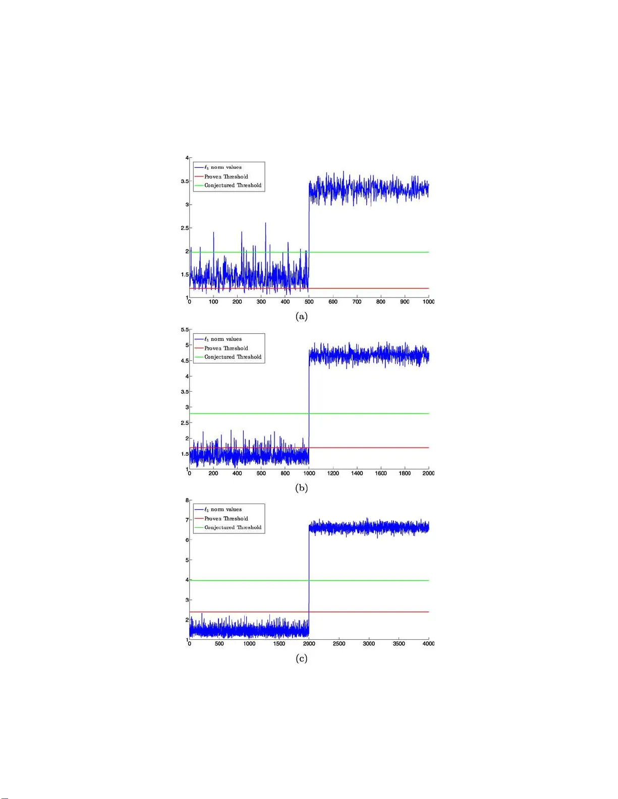
The Annals of Statistics 2012, V ol. 40, No. 4, 2195–22 38 DOI: 10.1214 /12-AOS1034 c  Institute of Mathematical Statistics , 2 012 A GEOMETRIC ANAL YSIS OF SUBSP A CE CLUSTERING WITH OUTLIERS By Mahdi Sol t anolkot abi 1 and Emmanuel J. Cand ´ es 2 Stanfor d University This pap er considers the problem of clustering a collection of un- labeled data p oints assumed to lie near a union of lo w er-dimensional planes. As is common in computer vision or u nsup ervised learning applications, we do not know in adv ance ho w many subspaces there are nor do we ha ve an y information about their d imensions. W e de- velo p a no vel geometric analysis of an algorithm named sp arse sub- sp ac e clustering (S SC) [In IEEE Confer enc e on Computer Vision and Pattern R e c o gnition, 2009. CVPR 2009 (2009) 2790–2797. IEEE], whic h signiﬁcantly broadens the range of problems where it is prov- ably eﬀectiv e. F or instance, w e sho w that SS C can reco ver multiple subspaces, eac h of dimension comparable to the ambient dimension. W e also prov e th at SS C can correctly cluster data p oin ts even when the su bspaces of interest inters ect. F urther, we d evelop an extension of SSC th at succeeds when the data set is corrupted with possibly o verwhelmingly many outliers. Und erlyin g our analysis are clear ge- ometric insigh ts, which may b ear on other sparse reco very problems. A numerical study complements our theoretical analysis and demon- strates t h e eﬀectiveness of these method s. 1. In tro duction. 1.1. Motivation. One of the m ost fundamental steps in data analysis and dimensionalit y reduction c onsists of appro ximating a giv en d ata s et by a single low-dimensional subsp ace, whic h is classica lly ac h iev ed via Principal Comp onent Analysis (PCA). In many problems, ho we ver, a collecti on of Received January 2012; revised July 2012. 1 Supp orted by a Benchmark Stanford Graduate F ellowship. 2 Supp orted in part by NSF via Grants CCF-0963835, CNS -0911041 and th e 2006 W a- terman Award, b y AFOSR under Gran t F A9550-09 -1-0643, and by ONR under Grant N00014-09-1-0258 . AMS 2000 sub je ct classiﬁc ations. 62-07. Key wor ds and phr ases. Su bspace clustering, sp ectral clustering, outlier detection, ℓ 1 minimization, duality in linear programming, geometric functional analysis, prop erties of conv ex b o d ies, concentration of measure. This is an electr onic reprint o f the original article published by the Institute of Mathematical Statistics in Th e Annals of Statistics , 2012, V ol. 40 , No. 4, 2195–22 3 8 . This reprint diﬀers from the o r iginal in pagination and typog raphic detail. 1 2 M. SOL T ANOLKOT ABI AND E. J. CAN D ´ ES Fig. 1. Col le ction of p oints ne ar a union of multiple sub sp ac es. p oin ts may not lie near a low-dimensional plane but near a union of multiple subspaces as sho wn in Figure 1 . It is then of in terest to ﬁnd or ﬁt all these subspaces. F urthermore, b ecause ou r data p oin ts are unlab eled in the sense that w e do not kno w in a dv ance to w h ic h subspace they b elong to, we need to simulta neously cluster these data into m ultiple s ubspaces and ﬁ nd a low- dimensional subsp ace appro ximating all the p oints in a cluster. This problem is kno wn as subsp ac e c lu stering and has n umerous applications; w e list just a few: • Unsup ervise d le arning . In u nsup ervised learning the goal is to build rep- resen tations of mac hine inp uts, whic h can b e used for decision making, predicting futur e inputs, eﬃcien tly comm unicating th e inputs to another mac hine and so on. In some u nsup ervised learnin g app licatio ns, the standard assump tion is that the data is w ell appro ximated b y a un ion of lo w er-dimensional man- ifolds. F urthermore, these manifolds are somet imes w ell appro ximated by subspaces whose d im en sion is only slightl y higher than that of the man- ifold under study . Suc h an example is handwritten d igits. When looking at h andwritten charac ters for recognition, the h uman ey e is ab le to al- lo w for simple transformations su c h as rotati ons, small sca lings, location shifts and charac ter thic kn ess. T herefore, any reasonable mo del should b e insensitiv e to su c h c h anges as w ell. Simard et al. [ 36 ] c h aracterize this in- v ariance with a 7-dimensional manifold; that is, diﬀeren t transformations of a single digit are we ll appro ximated by a 7-dimensional man if old. As illustrated b y Hastie et al. [ 17 ], these 7-dimensional manifolds are in turn w ell app ro ximated b y 12-dimensional subspaces. Thus, in certain cases, unsup ervised learning can b e formulated as a subs p ace clustering problem. • Computer vision . There has b een an explosion of visual data in the past few y ears. Cameras are now ev erywh ere: street corners, traﬃc ligh ts, air- SUBSP ACE CLUS TERING WITH OU TLIERS 3 p orts and so on. F ur thermore, millions of videos and images a re uploaded mon thly on the web. This visual data deluge has motiv ated the deve lop- men t of lo w-dimensional represen tations based on app earance, geometry and dynamics of a scene. In many su c h applicati ons, the lo w-dimensional represent ations a re c h aracterize d by m ultiple lo w-dimensional subspaces. One suc h example is motion segmentat ion [ 45 ]. Here, we hav e a video sequence which consists of multiple mo ving ob jects, and th e goal is to segmen t the tra jectories of the ob jects. Eac h tra jectory ap p ro ximately lies in a lo w-dimensional sub space. T o und erstand scene dynamics, on e needs to cluster the tra jectories of p oin ts on m o ving ob j ects based on the subspaces (ob jects) th ey b elong to, hence the need for su bspace clustering. Other applications of sub space clusterin g in compu ter vision include image segmen tation [ 48 ], face clus terin g [ 18 ], image repr esen tation and compression [ 19 ], and sys tems theory [ 44 ]. O ver the y ears, v arious metho ds for subs p ace clustering hav e b een prop osed by researc hers working in this area. F or a comprehen s iv e review and comparison of these algorithms, w e refer the reader to the tu torial [ 42 ] and references therein [ 1 , 4 , 5 , 9 – 12 , 14 , 16 , 28 , 30 , 31 , 34 , 37 , 38 , 40 , 43 , 47 , 49 – 51 ]. • Dise ase dete ction . In order to detect a class of diseases of a sp eciﬁc kind (e.g., metab olic), do ctors screen sp eciﬁc factors (e.g., m etabolites). F or this pu r p ose, v arious tests (e.g., blo o d tests) are p erformed on the new- b orns and the lev el of th ose factors are measur ed. One can f urther con- struct a newb orn-factor lev el matrix, where eac h ro w con tains the fac tor lev els of a diﬀerent n ewb orn. That is to sa y , eac h newb orn is associated with a v ector con taining the v alues of th e factors. Do ctors wish to cluster groups of newb orns based on the disease they suﬀer from. Usually , eac h disease c auses a correlation b et w een a sp eciﬁc s et of factors. Suc h an as- sumption imp lies that p oin ts corresp on d ing to newb orns suﬀering from a giv en disease lie on a lo w er-dimensional subspace [ 26 ]. Th erefore, the clustering of newb orns b ased on their sp eciﬁc disease together with the iden tiﬁcation of th e relev ant factors asso ciated with eac h disease can b e mo deled as a subsp ace clustering pr ob lem. PCA is p erhaps the single most imp ortant to ol for dimensionalit y re- duction. Ho we ve r, in man y problems, the data set un der study is not wel l appro ximated by a linear subspace of lo w er d imension. Instead, as w e hop e w e ha v e made clear, the data often lie n ear a union of lo w-dimensional sub- spaces, reﬂecting the multiple catego ries or classes a set of observ atio ns may b elong to. Giv en its r elev ance in data analysis, we ﬁnd it surpr ising that sub - space clustering has b een w ell s tudied in the computer s cience literature b ut has comparably receiv ed little atten tion from th e statistical comm unit y . This pap er b egins w ith a v ery recen t approac h to sub s pace clustering and p r o- p oses a framew ork in which one can dev elop some usefu l statistica l theory . 4 M. SOL T AN OLKOT ABI AND E. J. CAN D ´ ES As we shall see, ins igh ts from sparse regression analysis in high d imensions— a sub ject that h as b een well dev eloped in the statistics literature in recent y ears—inform th e sub space clustering problem. 1.2. Pr oblem formulation. In this pap er we assum e we are giv en data p oin ts that are distrib uted on a union of unknown linear su bspaces S 1 ∪ S 2 ∪ · · · ∪ S L ; that is, there are L subsp aces o f R n of unkn o wn dimensions d 1 , d 2 , . . . , d L . More p recisely , w e ha v e a p oin t set X ⊂ R n consisting of N p oin ts in R n , whic h may b e partitioned as X = X 0 ∪ X 1 ∪ · · · ∪ X L (1.1) for eac h ℓ ≥ 1, X ℓ is a collection of N ℓ unit-normed v ectors c hosen fr om S ℓ . The careful reader will notice that w e hav e an extra subset X 0 in ( 1.1 ) accoun ting f or p ossible outliers. Unless sp eciﬁed otherwise, w e assume that this sp ecial sub s et consists of N 0 p oin ts c hosen ind ep endent ly and u niformly at random on the unit sphere. The task is now simply stated. Without an y prior kno wledge ab out the n umb er of subs paces, their orien tation or their dimension, (1) iden tify all the outliers, and (2) segmen t or assign eac h d ata p oin t to a cluster as to reco ve r all the hidden subsp aces. It is worth emp hasizing th at our m o d el assu mes normalized data ve ctors; this is n ot a restrictiv e assump tion since one can alw a ys normalize inputs b efore applying any su bspace clustering algorithm. Although we consid er linear subs p aces, one can extend the metho ds of this pap er to aﬃn e subspace clustering whic h will b e explained in Section 1.3.1 . W e no w tu rn to methods for ac hieving these go als. Our f o cus is on noise- less data and w e lea v e noisy subspace clustering to future w ork. 1.3. Metho ds and c ontributions. T o in tro duce our metho ds , w e ﬁrst con- sider the case in which there are no outliers b efore treating the more general case. F r om now on, it w ill b e con v enient to arran ge the observ ed data p oint s as columns of a matrix X = [ x 1 , . . . , x N ] ∈ R n × N , wh ere N = N 0 + N 1 + · · · + N L is the total n umb er of p oin ts. 1.3.1. Metho ds. S ubspace clustering has r eceiv ed quite a bit of attenti on in r ecen t y ears and , in particular, Elhamifar and Vidal introdu ced a clev er algorithm based on insights from the c ompr essive sensing literature. The k ey idea of the Sparse Subspace Clustering (SSC) alg orithm [ 11 ] is to ﬁnd the sp arsest expansion of eac h column x i of X as a linear com bination of all the other co lumns . This mak es a lot of sense b ecause u nder some ge neric conditions, one exp ects that the sp arsest repr esen tation of x i w ould only SUBSP ACE CLUS TERING WITH OU TLIERS 5 select v ectors from the sub space in which x i happ ens to lie in. Th is motiv ates Elhamifar and Vidal to consider the sequence of optimization p roblems min z ∈ R N k z k ℓ 1 sub ject to Xz = x i and z i = 0 . (1.2) The hope is that whenev er z j 6 = 0, x i and x j b elong to the same subsp ace. This prop erty is captur ed by the deﬁnition b elo w. Definition 1.1 ( ℓ 1 subspace detection prop erty). The subspaces { S ℓ } L ℓ =1 and p oints X ob ey th e ℓ 1 subspace detection prop ert y if and on ly if it holds that for all i , the optimal solution to ( 1.2 ) has nonzero en tries only when the corresp ondin g columns of X are in the same subspace as x i . In certain cases the subspace detection prop ert y ma y not hold, that is, the supp ort of the optimal solution to ( 1.2 ) ma y include p oin ts from other subspaces. Ho w ev er, it might still b e p ossib le to d etect and construct re- liable clusters. A strategy is to arrange the optimal solutions to ( 1.2 ) as columns of a m atrix Z ∈ R N × N , build an aﬃnity graph G with N v ertices and weigh ts w ij = | Z ij | + | Z j i | , construct the normalized L ap lacian of G , and use a gap in the d istribution of eigen v alues of this matrix to estimate the num b er of su b spaces. Using the estimated num b er of subsp aces, sp ectral clustering tec hn iques (e .g., [ 33 , 35 ]) can b e applied to th e aﬃnit y graph to cluster the data p oint s. Th e main steps of this pr o cedu r e are summarized in Algorithm 1 . This algorithm clusters linear sub spaces but can also cluster aﬃne subsp aces by adding the constrain t Z T 1 = 1 to ( 1.2 ). 1.3.2. Our c ontributions. In S ection 3 we will r eview existing co nditions in v olving a restriction on th e minimum angle b etw een su b spaces un d er whic h Algorithm 1 is expected to work. The main purp ose of th is p ap er is to sh o w that Algorithm 1 w orks in muc h broader situations. • Subsp ac es with nontrivial interse ctions. Pe rhap s u nexp ectedly , w e shall see that our results assert that SS C can correctly cluster data p oin ts ev en w hen our subspaces inte rsect so that the minimum principal angle v anish es. T h is is a phenomenon w hic h is far from b eing explained by current theory . • Subsp ac es of ne arly line ar dimension. W e pro ve that in generic settings, SSC ca n eﬀectiv ely cluster the data ev en wh en the dimensions of the subspaces gro w almost linearly with the am bient dimension. W e are not a w are of other literature explaining w h y this should b e so. T o b e sur e, in most fa v orable cases, earlier resu lts only seem to allo w the dimensions of the subspaces to gro w at most lik e the square ro ot of the am b ien t dimension. • Outlier dete ction. W e present mo diﬁcations to SS C that succeed when the d ata set is corrup ted with man y outliers—ev en when their n umb er far exceeds the total num b er of clean observ ations. T o the b est of our 6 M. SOL T AN OLKOT ABI AND E. J. CAN D ´ ES Algorithm 1 Sparse sub s pace cl ustering (SSC ) Input: A data set X arranged as columns of X ∈ R n × N . 1. Solv e (the optimization v ariable is the N × N matrix Z ) minimize k Z k ℓ 1 sub ject to XZ = X , diag( Z ) = 0 . 2. F orm the a ﬃnity graph G w ith nodes representing the N data p oin ts and edge w eigh ts g ive n b y W = | Z | + | Z | T . 3. Sort the eigen v alues σ 1 ≥ σ 2 ≥ · · · ≥ σ N of the normalized Laplacian of G in descendin g order, and set ˆ L = N − arg max i =1 ,...,N − 1 ( σ i − σ i +1 ) . 4. Apply a sp ectral clus tering tec hn ique to the aﬃn it y graph using ˆ L as the estimated n umb er of clusters. Output: Pa rtition X 1 , . . . , X ˆ L . kno wledge, this is the ﬁrst algo rithm p ro v ably capable of h an d ling th ese man y corrup tions. • Ge ometric insights. Su c h imp ro v emen ts are p ossible b ecause of a no v el approac h to analyzing the sparse su bspace clustering problem. This a nal- ysis com bines to ols from con v ex optimiza tion, p robabilit y theory and ge- ometric functional analysis. Underlying our metho ds are clea r geometric insigh ts explaining qu ite pr ecisely when SSC is successful and when it is not. This viewp oin t migh t prov e f ruitful to address other sparse reco ve ry problems. Section 3 prop oses a careful comparison with th e existing literature. Be- fore doing so, we ﬁ rst need to introduce our results, whic h is the ob ject of Sections 1.4 and 2 . 1.4. Mo dels and typ ic al r esults. 1.4.1. Mo dels. In order to b etter understand the regime in w h ic h S SC succeeds as w ell as its limitations, we will consider three diﬀerent mo dels. Our aim is to giv e informativ e b ounds for these mo dels highligh ting the de- p endence up on key parameters of the p r oblem suc h as (1) the num b er of subspaces, (2) the dimensions of these s ubspaces, (3) the relativ e orient a- tions of these su bspaces, (4) the num b er of data p oints p er su b space and so on. SUBSP ACE CLUS TERING WITH OU TLIERS 7 • Deterministic mo del. In th is mo del the orienta tion of the sub spaces as w ell as the distribution of the p oin ts on eac h su bspace are nonrandom. This is the setting considered by Elhamifar et al. and is the sub ject of Theorem 2.5 , whic h guaran tees that the subsp ace detection prop ert y holds as long as for an y t w o sub spaces, pairs of (p rimal and dual) directions tak en on eac h subspace h a v e a suﬃ ciently small inner pro duct. • Semi-r andom mo del. Here, the sub spaces are ﬁxed bu t th e p oin ts are dis- tributed at rand om on eac h of the sub spaces. This is the sub ject of The- orem 2.8 , whic h uses a notion of aﬃnit y to measure closeness b et wee n an y t wo subspaces. This aﬃnit y is maximal and equal to the squ are root of the d imension of the su bspaces when they ov erlap p erfectly . Here, our results state that if the aﬃnit y is smaller, b y a logarithmic factor, than its maxim um p ossible v alue, then SSC reco v ers the su bspaces exac tly . • F ul ly r andom mo del. He re, b oth the orien tation of the sub spaces and th e distribution of the p oints are rand om. T his is the sub ject of Th eorem 1.2 ; in a nutshell, SSC s u cceds as long as the dimensions of the subsp aces are within at most a logarithmic factor from the ambien t dimension. 1.4.2. Se g mentation without outliers. Consider the fu lly random mo del ﬁrst. W e establish that the su bspace detection prop ert y holds as long as the dimensions of the subsp aces are roughly linear in the am bien t dim en sion. Put diﬀeren tly , SSC can prov ably ac hiev e p erfect subspace reco v ery in settings not previously und ersto o d . Our r esults mak e use o f a constant c ( ρ ) only dep ending up on the densit y of inliers (the num b er of p oints on eac h sub space is ρd + 1 ) a nd wh ic h ob eys the follo wing tw o prop erties: (i) F or all ρ > 1, c ( ρ ) > 0. (ii) There is a n umerical v alue ρ 0 , suc h that for all ρ ≥ ρ 0 , one can ta ke c ( ρ ) = 1 √ 8 . Theorem 1.2. Assume ther e ar e L subsp ac es, e ach of dimension d , chosen indep endently and u niformly at r andom. F urthermor e, supp ose ther e ar e ρd + 1 p oints chosen indep endently and unif ormly at r andom on e ach subsp ac e. 3 Then the subsp ac e dete ction pr op erty holds with lar ge pr ob ability as long as d < c 2 ( ρ ) log ρ 12 log N n (1.3) 3 F rom here on, when w e say that p oin ts are chosen from a subspace, w e implicitly assume they are un it normed. F or ease of presentation we state our results for 1 < ρ ≤ e d/ 2 , that is, the number of points on each subspace is not exponentially large in terms of the dimension of that subspace. The results h old for all ρ > 1 by replacing ρ with min { ρ, e d/ 2 } . 8 M. SOL T AN OLKOT ABI AND E. J. CAN D ´ ES [ N = L ( ρd + 1) is the to tal numb er of data p oints]. The pr ob ability is at le ast 1 − 2 N − N e − √ ρd , which is c alculate d for values of d close to the upp er b ound. F or low er values of d , the pr ob ability of su c c ess is of c ourse much higher, as explaine d b elow. Theorem 1.2 is in fact a sp ecial instance of a m ore general theorem that w e shall discuss later and whic h holds u nder less restrictive assu mptions on the orientati ons of the su bspaces as well as th e n umb er and p ositions of the d ata p oin ts on eac h sub space. This theorem conform s to our in tuition since clustering b ecomes more diﬃcult as th e dimensions of th e subsp aces increase. Intuitiv ely , another diﬃcult regime concerns a situation in which w e h a v e very many su bspaces of small dimensions. This diﬃcu lty is reﬂected in the d ep endence of the d enominator in ( 1.3 ) on L , the num b er of subs paces (through N ). A more comprehensive explanation of this eﬀect is pro vided in Section 2.1.2 . As it b ecomes cl ear in the pro of (see Secti on 7 ), a sligh tly more general v ersion of Theorem 1.2 holds, namely , with 0 < β ≤ 1, the su bspace detection prop erty h olds as long as d < 2 β  c 2 ( ρ ) log ρ 12 log N  n (1.4) with p robabilit y at least 1 − 2 N − N e − ρ (1 − β ) d . Th erefore, if d is a small fraction of the righ t-hand side in ( 1.3 ), the subspace detectio n prop ert y holds w ith m uc h higher probabilit y , as exp ected. An int eresting regi me is wh en the num b er of subspaces L is ﬁ xed and the densit y of p oints p er su bspace is ρ = d η , for a small η > 0 . Then as n → ∞ with the rati o d/n ﬁxed, it follo ws from N ≍ Lρd and ( 1.4 ) usin g β = 1 th at the subsp ace d etecti on prop ert y holds as long as d < η 48(1 + η ) n. This justiﬁes our earlier claims since w e can ha ve su bspace d imensions gro w- ing linearly in th e am bient dimension. It should be noted that this asymp- totic statemen t is only a f actor 8 − 10 a wa y from what is obs erv ed in sim- ulations, whic h demonstrates a relativ ely small gap b etw een our theoretical predictions and sim ulations. 4 1.4.3. Se g mentation with outliers. W e no w turn our atten tion to the case where there our extraneous p oints in th e data in the sen se that there are N 0 outliers assumed to b e distrib uted uniformly at random on the unit sphere. Here, w e wish to correct ly id en tify the outlier points and app ly a ny of th e subspace clustering algorithms to the remaining samples. W e p rop ose a v ery 4 T o b e concrete, when th e ambien t dimension is n = 50 and the number of subspaces is L = 10, the su b space detection prop erty holds for d in th e range from 7 to 10. SUBSP ACE CLUS TERING WITH OU TLIERS 9 Algorithm 2 Subs p ace clus tering in the presence of outliers Input: A data set X arranged as columns of X ∈ R n × N . 1. Solv e minimize k Z k ℓ 1 sub ject to XZ = X , diag( Z ) = 0 . 2. F or eac h i ∈ { 1 , . . . , N } , declare i to b e an outlier iﬀ k z i k ℓ 1 > λ ( γ ) √ n . 5 3. Apply a subsp ace clusterin g to the remaining p oin ts. Output: Pa rtition X 0 , X 1 , . . . , X L . simple detect ion p ro cedure f or this task. As in SSC, decompose eac h x i as a linear com bination of all th e other p oin ts by solving an ℓ 1 -minimization problem. Then one exp ects the expansion of an outlier to b e less sparse. This suggest s the follo w ing detection rule: declare x i to b e an outlier if and only if the optimal v alue of ( 1.2 ) is ab ov e a ﬁxed threshold. This makes sense b ecause if x i is an outlier, one exp ects the optimal v alue to b e on the order of √ n (p ro vided N is at most p olynomial in n ), whereas this v alue will be at most on the order of √ d if x i b elongs to a subspace of dimens ion d . In short, w e exp ect a gap—a fact we will make rigorous in the next section. The main steps of the pro cedur e are sh o wn in Algorithm 2 . Our second result asserts that as long as the num b er of outliers is not o v erwhelming, Alg orithm 2 detects all of them. Theorem 1.3. Assume ther e ar e N d p oints to b e cluster e d to gether with N 0 outliers sample d uniformly at r andom on the n − 1 - dimensional uni t spher e ( N = N 0 + N d ). Algorithm 2 dete cts al l of the outliers with high pr ob- ability 6 as long as N 0 < 1 n e c √ n − N d , wher e c is a numeric al c onstant. F urthermor e, supp ose the subsp ac es ar e d -dimensional and of arbitr ary orientation, and that e ach c ontains ρd + 1 p oints sample d indep e ndently and u niformly at r andom . Then with high pr ob- ability, 7 Algor ithm 2 do es not dete c t any subsp ac e p oint as outlier pr ovide d 5 Here, γ = N − 1 n is t he to tal p oint density and λ is a threshold ratio function whose v alue shall b e discussed later. 6 With probability at least 1 − N 0 e − C n/ log( N 0 + N d ) . If N 0 < 1 n e c √ n − N d , th is is at least 1 − 1 n . 7 With probabilit y at least 1 − N 0 e − C n/ log( N 0 + N d ) − N d e − √ ρd . If N 0 < min { ne c 2 n/d , 1 n e c √ n } − N d , this is at least 1 − 1 n − N d e − √ ρd . 10 M. SOL T AN OLKOT ABI AND E. J. CAN D ´ ES that N 0 < nρ c 2 n/d − N d , in which c 2 = c 2 ( ρ ) / (2 e 2 π ) . This r esu lt sho ws th at our outlier detection scheme can reliably detect all outliers ev en when their n umb er g rows exponentiall y in th e root of the am bien t dimension. W e emphasize that this h olds without making an y as- sumption w hatsoever ab out the orien tatio n of the subspaces or the distri- bution of the p oin ts on eac h subspace. F urthermore, if the p oin ts on eac h subspace are u niformly d istr ibuted, our sc h eme will not wron gfu lly d etect a subspace p oin t as an outlier. In th e n ext section we sh o w that similar results hold under less restrictiv e assu mptions. 2. Main results. 2.1. Se gmentation without outliers. In this section w e shall giv e su ﬃ cien t conditions in the fully d etermin istic and semi-random mo d el und er wh ic h the SSC algorithm succeeds (w e studied the fully rand om mo del in Theorem 1.2 ). Before we explain our results, we int ro du ce some b asic notation. W e will arrange the N ℓ p oin ts on su bspace S ℓ as columns of a matrix X ( ℓ ) . F or ℓ = 1 , . . . , L , i = 1 , . . . , N ℓ , w e use X ( ℓ ) − i to denote all p oints on su b- space S ℓ excluding the i th p oint, X ( ℓ ) − i = [ x ( ℓ ) 1 , . . . , x ( ℓ ) i − 1 , x ( ℓ ) i +1 , . . . , x ( ℓ ) N ℓ ]. W e u s e U ( ℓ ) ∈ R n × d ℓ to denote an arbitrary orthonormal basis for S ℓ . This in duces a factorizatio n X ( ℓ ) = U ( ℓ ) A ( ℓ ) , where A ( ℓ ) = [ a ( ℓ ) 1 , . . . , a ( ℓ ) N ℓ ] ∈ R d ℓ × N ℓ is a matrix of co ordin ates with unit-norm columns. F or any matrix X ∈ R n × N , the shorthand notation P ( X ) denotes the symmetrized con v ex hull of its columns, P ( X ) = con v ( ± x 1 , ± x 2 , . . . , ± x N ). Also P ℓ − i stands for P ( X ( ℓ ) − i ). Finally , k X k is the op erator norm of X and k X k ℓ ∞ the maximum absolute v alue of its entries. 2.1.1. Deterministic mo del. W e ﬁrst in tro duce some basic concepts needed to state our deterministic result. Definition 2.1 (Dual p oin t). Consider a v ector y ∈ R d and a matrix A ∈ R d × N , and let C ∗ b e the set of optimal solutions to max λ ∈ R d h y , λ i sub j ect to k A T λ k ℓ ∞ ≤ 1 . The dual p oint λ ( y , A ) ∈ R d is d eﬁned as a p oint in C ∗ with minim um Euclidean norm. 8 A geometric representa tion is sh o wn in Figure 2 . 8 If this p oint is not uniq u e, t ak e λ ( y , A ) to b e any optimal p oint with minim um Euclidean norm. SUBSP ACE CLUS TERING WITH OU TLIERS 11 Fig. 2. Ge ometric r epr esentation of a dual p oint; se e Deﬁni tion 2.1 . Definition 2.2 (Dual directions). Deﬁne the dual directions v ( ℓ ) i ∈ R n [arranged as columns of a matrix V ( ℓ ) ] corresp ond ing to the dual p oin ts λ ( ℓ ) i = λ ( a ( ℓ ) i , A ( ℓ ) − i ) as v ( ℓ ) i = U ( ℓ ) λ ( ℓ ) i k λ ( ℓ ) i k ℓ 2 . The dual direction v ( ℓ ) i , corresp onding to the p oint x ( ℓ ) i , from sub s pace S ℓ is sho wn in Figure 3 . Definition 2.3 (Inradius). The inradiu s of a con ve x b o dy P , denoted b y r ( P ), is deﬁned as the radiu s of th e largest Euclidean ball inscrib ed in P . Fig. 3. G e ometric r epr esentation of a dual dir e ction. The dual dir e ction i s the dual p oint emb e dde d in the ambient n -dimensional sp ac e. 12 M. SOL T AN OLKOT ABI AND E. J. CAN D ´ ES Definition 2.4 (Sub space in coherence). The subspace incoherence of a p oin t set X ℓ vis a vis the other p oint s is deﬁ ned b y µ ( X ℓ ) = max x ∈X \X ℓ k V ( ℓ ) T x k ℓ ∞ , where V ( ℓ ) is as in Deﬁnition 2.2 . Theorem 2.5. If µ ( X ℓ ) < min i : x i ∈X ℓ r ( P ℓ − i ) (2.1) for e ach ℓ = 1 , . . . , L , then the subsp ac e dete ction pr op erty holds. If ( 2.1 ) holds for a given ℓ , then a lo c al subsp ac e dete ction pr op erty holds in the sense that for al l x i , the solution to ( 1.2 ) has non zer o entries only when the c orr esp onding c olumns of X ar e in the same subsp ac e as x i . The incoherence parameter of a set of p oin ts on one subsp ace with resp ect to other p oin ts is a measure of aﬃnit y b etw een subspaces. T o see why , notice that if the incoherence is h igh, it implies that there is a p oint on one su bspace and a d irection on another (a d ual direction) su ch that the angle b et w een them is small. That is, there are t wo “close” subsp aces, h ence, clustering b ecomes hard. The inradius measures the spr ead of p oints. A v ery small minimum inradius implies that the distribution of p oint s is sk ewe d to w ard certain directions, thus, su bsp ac e clustering using an ℓ 1 p enalt y is diﬃcult. T o see wh y this is so, assume the subspace is of dimension 2 and all of th e p oin ts on the subs pace are skew ed to w ard one line, except f or one sp ecial p oint whic h is in the direction orthogonal to that line. This is sho wn in Figure 4 with the s p ecial p oin t in red and the others in blu e. T o syn thesize th is sp ecial p oin t as a linear com bination of the other p oints from its subspace, w e w ould need h uge coeﬃcien t v alues and this is why it may v ery well b e more economic al—in an ℓ 1 sense—to select p oin ts from other subspaces. Th is is a situation w here ℓ 0 minimization would still b e successful but its con v ex s u rrogate is not (resea rchers familiar with sparse regression w ould r ecognize a setting in w h ic h v ariables are correlated and whic h is Fig. 4. Skewe d distribution of p oints on a single subs p ac e and ℓ 1 synthesis. SUBSP ACE CLUS TERING WITH OU TLIERS 13 c hallenging for th e LASSO). Theorem 2.5 essen tially state s that as long as diﬀeren t subspaces are not similarly orien ted and the p oints on a single subspace are wel l spread, SSC can cluster the data correctly . A geometric p ersp ectiv e of ( 2.1 ) is provided in Secti on 4 . T o get concrete results, one needs to estimate b oth the incoherence and inradius in terms of the parameters of interest, wh ic h include the num b er of subspaces, the dimens ions of th e subsp aces, the num b er of p oin ts on eac h subspace and so on. T o do this, w e u se the p r obabilistic mo dels we in tro du ced earlier. This is our next topic. 2.1.2. Semi-r ando m mo del. The follo wing deﬁnitions capture notions of similarit y/aﬃnit y betw een t w o sub spaces. Definition 2.6. The principal angles θ (1) k ,ℓ , . . . , θ ( d k W d ℓ } k ,ℓ b et w een t wo subspaces S k and S ℓ of dimensions d k and d ℓ are recursive ly deﬁ ned b y cos( θ ( i ) k ℓ ) = max y ∈ S k max z ∈ S ℓ y T z k y k ℓ 2 k z k ℓ 2 := y T i z i k y i k ℓ 2 k z i k ℓ 2 , with the orthogonalit y constraints y T y j = 0, z T z j = 0, j = 1 , . . . , i − 1. Alternativ ely , if the columns of U ( k ) and U ( ℓ ) are orthobases, then the co- sine of the principal angles are th e singu lar v alues of U ( k ) T U ( ℓ ) . W e write the smallest p rincipal angle as θ k ℓ = θ (1) k ℓ so that cos( θ k ℓ ) is the largest s ingular v alue of U ( k ) T U ( ℓ ) . Definition 2.7. The aﬃnit y b et w een tw o subsp aces is deﬁned b y aﬀ ( S k , S ℓ ) = q cos 2 θ (1) k ℓ + · · · + cos 2 θ ( d k W d ℓ ) k ℓ . In case the distribu tion of the p oin ts are unif orm on their corresp ond- ing su bspaces, the Geometric Cond ition ( 2.1 ) may b e reduced to a simple statemen t ab out the aﬃnit y . Th is is the sub ject of the next theorem. Theorem 2.8. Supp ose N ℓ = ρ ℓ d ℓ + 1 p oints ar e chosen on e ach sub- sp ac e S ℓ at r andom, 1 ≤ ℓ ≤ L . Then as long as max k : k 6 = ℓ 4 √ 2(log[ N ℓ ( N k + 1)] + log L + t ) aﬀ ( S k , S ℓ ) √ d k (2.2) < c ( ρ ℓ ) p log ρ ℓ for e ach ℓ, the subsp ac e dete ction pr op erty hold s with pr ob ability at le ast 1 − L X ℓ =1 N ℓ e − √ d ℓ √ N ℓ − 1 − 1 L 2 X k 6 = ℓ 4 e − 2 t ( N k + 1) N ℓ . 14 M. SOL T AN OLKOT ABI AND E. J. CAN D ´ ES Henc e, ignoring lo g f actors, subsp ac e clustering is p ossible if the aﬃnity b etwe en the subsp ac es is less than ab out the squar e r o ot of the dimension of these subsp ac es. T o deriv e useful resu lts, assume for simp licit y that w e ha ve L s ubspaces of the same dimension d and ρd + 1 p oin ts p er su bspace so that N = L ( ρd + 1). Then p erfect clustering o ccurs with probabilit y at least 1 − N e − √ ρd − 2 ( ρd )( ρd +1) e − 2 t if aﬀ ( S k , S ℓ ) √ d < c ( ρ ) √ log ρ 4 √ 2(2 log N + t ) . (2.3) Our notion of aﬃnit y matc hes ou r basic intuition. T o b e sure, if the sub- spaces are to o close to eac h other (in terms of our deﬁ n ed n otion of aﬃn it y), subspace clustering is hard. Ha ving said th is, our result has an element of surpr ise. In deed, the aﬃnity can at m ost b e √ d ( √ d k in general) and, there- fore, our result essent ially states that if the aﬃnit y is less th an c √ d , then SSC works. No w this allo ws for subspaces to in tersect and, y et, SSC still pro v ably clusters all the data p oin ts correctly! T o d iscu ss other asp ects of this result, assume as b efore that all sub- spaces ha ve the same dimen s ion d . When d is sm all and the total n umb er of subsp aces is O ( n/d ), the pr oblem is inheren tly hard b ecause it inv olv es clustering al l the p oin ts in to many small subgroups. This is r eﬂected by the lo w p robabilit y of success in Theorem 2.8 . Of cour s e, if one increases the n umb er of p oint s chosen fr om eac h subspace, the prob lem should intuitiv ely b ecome easier. The p robabilit y asso ciated with ( 2.3 ) allo ws for suc h a trend. In other w ords, when d is small, o ne can increase the p robabilit y of success b y in cr easing ρ . In tro du cing a parameter 0 < β ≤ 1, the condition can b e mo diﬁed to aﬀ ( S k , S ℓ ) √ d < c ( ρ ) √ β log ρ 4(2 log N + t ) , (2.4) whic h h olds with p robabilit y at least 1 − N e − ρ (1 − β ) d − 2 ( ρd )( ρd +1) e − 2 t . Th e more general co ndition ( 2.2 ) and the corresp onding probabilit y can also b e mo diﬁed in a similar manner. 2.2. Se gmentation with outliers. T o see ho w Algorithm 2 w orks in the presence of outliers, we b egin by in tro ducing a prop er threshold fun ction and deﬁne λ ( γ ) =          r 2 π 1 √ γ , 1 ≤ γ ≤ e, r 2 π e 1 √ log γ , γ ≥ e, (2.5) SUBSP ACE CLUS TERING WITH OU TLIERS 15 Fig. 5. Plot of the thr eshold f unction ( 2.5 ). sho wn in Figure 5 . The theorem b elo w justiﬁes the claims made in the in tro duction. Theorem 2.9. Supp ose the outlier p oints ar e c hosen uniformly at r an- dom and set γ = N − 1 n , then using the thr eshold value (1 − t ) λ ( γ ) √ e √ n , al l outliers ar e identiﬁe d c orr e ctly with pr ob ability at le ast 1 − N 0 e − C 1 t 2 n/ log N for some p ositive numeric al c onstant C 1 . F urthermor e, we have the fol lowing guar ante es in the deterministic and semi-r ando m mo dels: (a) If in the deterministic mo del, max ℓ,i 1 r ( P ( X ( ℓ ) − i )) < (1 − t ) λ ( γ ) √ e √ n, (2.6) then no “r e al” data p oint is wr ongful ly dete cte d as an outlier. (b) If in the semi-r andom mo del, max ℓ √ 2 d ℓ c ( ρ ℓ ) √ log ρ ℓ < (1 − t ) λ ( γ ) √ e √ n, (2.7) then with pr ob ability at le ast 1 − P L ℓ =1 N ℓ e − √ d ℓ √ ( N ℓ − 1) , no “r e al” da ta p oint is wr ongfu l ly dete cte d as an outlier. The threshold in th e righ t-hand side of ( 2.6 ) and ( 2.7 ) is essentia lly √ n m ultiplied by a factor whic h dep end s only on the ratio of the num b er of p oin ts and the dimens ion of the am b ien t space. As in the situation with no outliers, when d ℓ is small we need to increase N ℓ to get a resu lt holding with high probabilit y . Again this is exp ected 16 M. SOL T AN OLKOT ABI AND E. J. CAN D ´ ES b ecause when d ℓ is small, we need to b e able to separate the outliers from man y small clus ters whic h is inherentl y a hard problem for small v alues of N ℓ . The careful reader will notice a factor √ e discrepancy b et w een the thresh- old λ ( γ ) √ n p resen ted in Algorithm 2 and what is pro v en in ( 2.6 ) and ( 2.7 ). W e b eliev e that this is a resu lt of our analysis 9 and we conjecture that ( 2.6 ) and ( 2.7 ) hold without the factor √ e in the d enominator. Our s imulations in Section 5 supp ort this conjecture. 3. Discussion and comparison with other w ork. It is time to compare our results with a couple of previous imp ortant theoretical adv ances. T o in tro duce these earlier works, w e ﬁrst need some deﬁnitions. Definition 3.1. T he subsp aces { S ℓ } L ℓ =1 are said to b e ind ep enden t if and only if P ℓ dim( S ℓ ) = d im( ⊕ ℓ S ℓ ), wher e ⊕ is the direct sum. F or instance, three lines in R 2 cannot b e indep endent. Definition 3.2. The su bspaces { S ℓ } L ℓ =1 are said to b e disjoin t if and only if for all pairs k 6 = ℓ , S k ∩ S ℓ = { 0 } . Definition 3.3. The geodesic d istance b etw een tw o subspaces S i and S j of dimension d , d enoted b y dist( S i , S j ), is d eﬁned b y dist( S k , S ℓ ) = v u u t d k W d ℓ X i =1 ( θ ( i ) k ℓ ) 2 . 3.1. Se gmentation without outliers. In [ 11 ], Elhamifar an d Vidal show that the s u bspace d etectio n prop erty holds as long as the su bspaces are indep endent. In [ 12 ], the same authors sh o w that un der less restrictiv e con- ditions the ℓ 1 subspace detection pr op ert y still holds. F ormally , they sho w that if 1 √ d ℓ max Y ∈ W d ℓ ( X ( ℓ ) ) σ min ( Y ) > m ax k : k 6 = ℓ cos( θ (1) k ℓ ) for all ℓ = 1 , . . . , L, (3.1) then the subspace detection pr op ert y holds. In th e ab o ve formulation, σ min ( Y ) denotes the smallest singular v alue of Y and W d ( X ( ℓ ) ) denotes the set of all fu ll rank sub-matrices of X ( ℓ ) of size n × d ℓ . The in teresting part of the ab o v e condition is the app earance of the principal angle on the righ t-hand side. Ho w ev er, the left-hand sid e is not particularly insigh tful (i.e., it do es not tell us an ything ab out the imp ortan t parameters inv olv ed in the sub- 9 More sp eciﬁcally , from switc hing from the mean width to a volumetric argument by means of Urysohn’s inequality . SUBSP ACE CLUS TERING WITH OU TLIERS 17 space clustering problem, suc h as dimensions, n umb er of s ubspaces and so on) and it is in fact NP-hard to ev en calculate it. • Deterministic mo del. T his pap er also introd uces a suﬃ cient condition ( 2.1 ) under whic h th e subspace detection prop erty holds in the fully determin- istic setting; compare Th eorem 2.5 . This suﬃcien t condition is muc h less restrictiv e as an y conﬁguration ob eying ( 3.1 ) also ob eys ( 2. 1 ). More p re- cisely , µ ( X ℓ ) ≤ max k : k 6 = ℓ cos( θ (1) k ℓ ) and 1 √ d ℓ max Y ∈ W d ℓ ( X ( ℓ ) ) σ min ( Y ) ≤ min i r ( P ℓ − i ). 10 As for ( 3.1 ), chec king that ( 2.1 ) h olds is also NP-hard in general. Ho w ev er, to pro v e that the subspace detection prop erty holds, it is suﬃcien t to c h ec k a sligh tly less restrictive condition than ( 2.1 ); this is tractable, see Lemma 7.1 . • Semi-r andom mo del. Assume that all subspaces are of the s ame dimension d and th at there are ρd + 1 p oints on eac h subs p ace. Since the columns of Y ha v e u nit norm, it is easy to see that the left-hand side of ( 3.1 ) is strictly less than 1 / √ d . Thus, ( 3.1 ) at b est restricts th e range for p erfect subspace reco ve ry to co s θ (1) k ℓ < c 1 √ d [b y lo oking at ( 3.1 ), it is not enti rely clear that this would ev en b e ac hiev able]. In comparison, Theorem 2.8 (excluding some logarithmic factors for ease of presentat ion) requires aﬀ ( S k , S ℓ ) = q cos 2 ( θ (1) k ℓ ) + cos 2 ( θ (2) k ℓ ) + · · · + cos 2 ( θ ( d ) k ℓ ) (3.2) < c p log( ρ ) √ d. The left-hand side can b e m uch smaller than √ d cos θ (1) k ℓ and is, therefore, less restrictiv e. T o b e more sp eciﬁc, assume that in th e m od el d escrib ed abov e w e ha v e tw o subsp aces with an intersectio n of dimension s . Because the tw o subspaces in tersect, the condition giv en b y Elhamifar and Vidal b ecomes 1 < 1 √ d , whic h cannot hold. In comparison, our condition ( 3 .2 ) simpliﬁes to cos 2 ( θ ( s +1) k ℓ ) + · · · + cos 2 ( θ ( d ) k ℓ ) < c log( ρ ) d − s, whic h holds as long as s is not to o large and/or a fraction of th e angles are not too sm all. F rom an application standp oint, this is imp ortan t b ecause it explains why SSC can often succeed ev en when the subspaces are not disjoin t. • F ul ly r ando m mo del. As b efore, assume for simp licit y that all subspaces are of the same dimension d and that there are ρd + 1 p oint s on eac h subspace. W e h a v e seen that ( 3.1 ) imp oses cos θ (1) k ℓ < c 1 √ d . It can b e s ho wn 10 The latter follo ws from max i 1 r ( P ℓ − i ) ≤ min Y ∈ W d ℓ ( X ( ℓ ) ) √ d ℓ σ min ( Y ) whic h is a simple con- sequence of Lemma 7.8 . 18 M. SOL T AN OLKOT ABI AND E. J. CAN D ´ ES that in the fully random setting, 11 cos θ (1) k ℓ ≈ c q d n . Th er efore, ( 3.1 ) would put a restriction of the form d < c √ n. In comparison, Theorem 1.2 requires d < c 1 log ρ log N n, whic h allo ws for the dimension of the su bspaces to b e a lmost linear in th e am bien t dimension. Suc h impro v emen ts come from a geometric in sigh t: it b ecomes appar- en t th at the SSC algorithm succeeds if th e actual subspace p oin ts (primal directions) hav e small inner pro d ucts with the dual directions on another subspace. This is in contrast with Elhamifar and Vidal’s condition whic h requires that the inn er pr o ducts b et wee n a ny direction on one subsp ace and any direction on another b e small. F urther geometric explanations are give n in Section 4.2 . 3.2. Se gmentation with outliers. T o the b est of our kno wledge, there is only one other theoretical result regarding outlier detection. In [ 27 ], Lerman and Zhan g study the eﬀectiv eness of r eco vering sub spaces in th e p resence of outliers by some sort of ℓ p minimization for diﬀeren t v alues of 0 < p < ∞ . They address sim ultaneous reco v ery of all L subsp aces by minimizing the functional e ℓ p ( X , S 1 , . . . , S L ) = X x ∈X min 1 ≤ ℓ ≤ L (dist( x , S ℓ )) p . (3.3) Here, S 1 , . . . , S L are the optimiza tion v ariables and X is our data set. This is not a conv ex optimization for any p > 0, since the feasible set is the Grassmannian. In the semi-random mo del, th e result of Lerman and Zh ang states that under the assumptions stated in Theorem 1.3 , with 0 < p ≤ 1 and τ 0 a constan t, 12 the su bspaces S 1 , . . . , S L minimize (with large probabilit y) the energy ( 3.3 ) among all d -dim en sional subspaces in R n if N 0 < τ 0 ρd m in  1 , min k 6 = ℓ dist( S k , S ℓ ) p / 2 p  . (3.4) 11 One can see this by noticing that t he square of this parameter is the largest root of a multiv ariate b eta distribut ion. The asymptotic v alue of this root ca n b e calculated, for example, see [ 21 ]. 12 The result of [ 27 ] is a b it more general in th at th e p oints on each sub space can b e sampled from a si ngle distribut ion ob eying certain regularit y conditions, other than the uniform measure. In this case, τ 0 dep ends on this d istribution as w ell. SUBSP ACE CLUS TERING WITH OU TLIERS 19 It is easy to see that the righ t-hand side of ( 3.4 ) is upp erb ounded b y ρd , that is, the t ypical num b er of p oint s on eac h subsp ace. Notice that our analogous result in Theorem 1.2 allo w s for a muc h larger n umb er of outliers. In f act, the n umb er of outliers can sometimes ev en b e m uc h larger than the total num b er of data p oint s on all subspaces com b ined. Our prop osed algorithm also has the added b eneﬁt that it is conv ex and , th er efore, practical. Ha ving said this, it is worth menti oning that the r esults in [ 27 ] hold for a more general outlier mo del. Also, an in teresting bypro duct of the r esult f rom Lerman and Z hang is that the energy min imizatio n can p erform p erfect subsp ace reco v ery w hen no outliers are present. In fact, they ev en extend this to the case wh en the subspace p oint s are noisy . Finally , while this manuscript was in prep aration, L iu Guangcan br ough t to ou r atten tion a new pap er [ 29 ], w h ic h also addresses outlier detection. Ho w ev er, the suggested sc heme limits the num b er of outliers to N 0 < n − P L ℓ =1 d ℓ . That is, when the total dimension of the subspaces ( P L ℓ =1 d ℓ ) ex- ceeds the ambien t dimension n , outlier detection is not p ossible based on the su ggeste d sc heme. In con trast, our results guarantee p erfect outlier de- tection eve n when the n umber of outliers far exceeds the num b er of data p oin ts. 4. Geometric p ersp ectiv e on the s eparation condition. The goal of th is section is t wofold. One aim is to provide a geometric understand ing of the subspace detection prop erty and of the suﬃcient condition presented in Sec- tion 2.1 . Another is to in tro duce concepts suc h as K -norms and p olar sets, whic h will play a crucial role in our analysis. 4.1. Line ar pr o gr amming the ory. W e are inte rested in ﬁ nding the sup- p ort of the optimal solution to min x ∈ R N k x k ℓ 1 sub ject to Ax = y , (4.1) where b oth y and th e columns of A h a v e unit norm. Th e dual tak es the form max z ∈ R n h y , z i sub ject to k A T z k ℓ ∞ ≤ 1 . (4 .2) Since strong dualit y alw a ys holds in linear programming, the optimal v alues of ( 4.1 ) and ( 4.2 ) are equal. W e no w int ro du ce some notati on to express the dual program diﬀeren tly . Definition 4.1. The norm of a v ector y with resp ect to a symmetric con v ex b o dy is deﬁned as k y k K = inf { t > 0 : y /t ∈ K} . (4.3) This norm is sho wn in Figure 6 (a). 20 M. SOL T AN OLKOT ABI AND E. J. CAN D ´ ES Fig. 6. Il lustr ation of Deﬁnitions 4.1 and 4.2 . (a) Norm wi th r esp e ct to a p olytop e K . (b) Polytop e K and i ts p olar K o . Definition 4.2. The p olar set K o of K ⊂ R n is deﬁned as K o = { y ∈ R n : h x , y i ≤ 1 for all x ∈ K} . (4.4) Set K o = { z : k A T z k ℓ ∞ ≤ 1 } so that our dual problem ( 4.2 ) is of th e form max z ∈ R n h y , z i su b ject to z ∈ K o . (4.5) It then follo ws from the deﬁnitions ab o v e that th e optimal v alue of ( 4.1 ) is giv en by k y k K , where K = conv( ± a 1 , . . . , ± a N ); that is to sa y , the m in im um v alue of the ℓ 1 norm is the n orm of y with resp ect to the symmetrized con v ex hull of the columns of A . In other words, this p ersp ectiv e asserts that supp ort detection in an ℓ 1 minimization pr oblem is equiv alen t to ﬁnding the face of the p olytop e K that passes thr ough the ra y ~ y = { t y , t ≥ 0 } ; the extreme p oin ts of this face revea l th ose indices with a nonzero en try . W e will r efer to th e face passing through the ray ~ y as the face closest to y . Figure 6 (b) illustrates some of these concepts. 4.2. A ge ometric view of the subsp ac e dete ction pr op e rty. W e ha v e seen that the su bspace detec tion prop erty holds if for eac h p oint x i , the closest face to x i resides in the same su bspace. T o establish a geometric charact er- ization, consider an arbitrary p oint, for instance, x ( ℓ ) i ∈ S ℓ as in Figure 7 . No w construct the symmetrized con v ex h ull of all the other p oin ts in S ℓ indicated by P ℓ − i in the ﬁ gure. Consider the f ace of P ℓ − i that is closest to x ( ℓ ) i ; this face is shown in Figure 7 by the line segmen t in red. Also, consider the plane p assing through this segment and orthogonal to S ℓ along with its reﬂection ab out the origin; this is shown in Figure 7 b y the ligh t grey p lanes. SUBSP ACE CLUS TERING WITH OU TLIERS 21 Fig. 7. I l lustr ation of ℓ 1 minimi zation when the subsp ac e dete ction pr op erty holds. Same obje ct se en fr om di ﬀer ent angles . Set R ( ℓ ) i to b e the regio n of sp ace r estricted b et w een these t w o planes. Intu- itiv ely , if no t w o points on the ot her subspaces lie outsid e of R ( ℓ ) i , then the face c hosen by the a lgorithm is a s in th e ﬁgur e and lies in S ℓ . T o illustrate this p oin t fu rther, supp ose there are t w o p oin ts n ot in S ℓ lying outside of the region R ( ℓ ) i as in Figure 8 . In this case, the close st face do es n ot lie in S ℓ as can b e seen in th e ﬁgure. Therefore, one could in tuitiv ely argue that a suﬃcient condition for the closest face to lie in S ℓ is that the pro jections ont o S ℓ of the p oints from all the other subspaces do not lie outside of regions R ( ℓ ) i for all p oints x ( ℓ ) i in subsp ace S ℓ . This Fig. 8. Il lustr ation of ℓ 1 minimi zation when the subsp ac e dete ction pr op erty fai ls. Same obje ct se en fr om di ﬀer ent angles . 22 M. SOL T AN OLKOT ABI AND E. J. CAN D ´ ES Fig. 9. Ge ometric view of ( 2.1 ). The right ﬁgur e i s se en fr om a dir e ction ortho gonal to S 1 . condition is closely related to the su ﬃcien t condition stated in Theorem 2.5 . More pr ecisely , the dual directions v ( ℓ ) i appro ximate the normal directions to the restricting planes R ( ℓ ) i , and min i r ( P ℓ − i ) the distance of these planes from the origin. Finally , to un derstand the s u ﬃcien t condition of Theorem 2.5 , we will use Figure 9 . W e fo cus on a single subspace, s a y , S 1 . As previously stated, a suﬃcien t condition is to h a v e all p oin ts not in S 1 to ha v e small coherence with the d u al directions of the p oints in S 1 . The dual directions are depicted in Figure 9 (b lue dots). One such dual directio n line is s h o wn as the d ash ed blue line in the ﬁgur e. The p oin ts that ha v e lo w coherence with the dual directions are the p oints whose pr o jection onto su bspace S 1 lie inside the red p olytop e. As can be s een, this p olytop e approximate s the int ersection of regions R (1) i ( T N 1 i =1 R (1) i ) and subspace S 1 . This helps in u n derstanding the diﬀerence b et wee n the condition imp osed b y Elhamifar and Vidal and our condition; in this s etting, th eir condition essentiall y states that the pro jec- tion of th e p oints on all other subsp aces on to subspace S 1 m ust lie in side the blue circle. By lo oking at Figure 9 , one migh t draw the conclusion that these conditions are v ery similar, that is, the red p olytop e an d the blue ball restrict almost the same region. This is not the case, because as the dimen - sion of the subspace S 1 increases most of the v olume of the red p olytop e will b e concen trated around its v ertices and the ball will only occupy a v ery small fraction of the total vo lume of the p olytop e. 5. Numerical results. Th is section prop oses n umerical exp erimen ts on syn thesized d ata to fur ther our u nderstanding of the b eha vior/limitations of SSC, of our analysis and of our prop osed outlier detection sc heme. In this n umerical study we restrict ourselv es to un derstanding the eﬀect of noise on th e sp ectral gap and the estimation of the n um b er of su b spaces. F or a more comprehensiv e analytical and numerical stud y of SSC in the presence SUBSP ACE CLUS TERING WITH OU TLIERS 23 of noise, w e refer the reader to [ 7 ]. F or comparison o f SSC with more recent metho ds on m otion segmenta tion data, we refer the r eader to [ 13 , 28 ]. These pap ers in dicate that SSC has the b est p erformance on the Hopkins 155 data [ 39 ] when corru pted tra jectories are pr esent, and h as a p erformance comp etitiv e with the state of the art when th ere is no corrupted tra jectory . In the sp irit of repro d ucible researc h, the Matla b co de generating all the plots is a v ailable at http://w ww.stanfor d.edu/ ~ mahdisol /Software . 5.1. Se gmentation without outliers. As men tioned in th e In tro du ction , the subspace detection prop ert y can hold ev en when the dimensions of the subspaces are large in comparison with the a mbien t d im en sion n . SS C can also wo rk b ey ond the region wher e the subspace detection pr op ert y h olds b e- cause of further sp ectral clustering. S ection 5.1.1 in tro duces sev eral metrics to assess p erformance and Section 5.1.2 demonstrates th at the subspace de- tection pr op ert y can hold ev en when th e subspaces intersect. In Section 5.1.3 w e s tu dy the p erformance of SSC u nder c hanges in the aﬃnit y b et w een sub- spaces and the num b er of p oin ts per subspace. In Section 5.1.4 we illustrate the eﬀect of the d imension of the subspaces on the su bspace detection prop- ert y and the s p ectral gap. I n Section 5.1.5 we study the eﬀect of noise on the sp ectral gap. In the ﬁnal su b section w e study the capability of SSC in estimating the correct num b er of subspaces and compare it with a classica l algorithm. 5.1.1. Err or metrics. Th e four diﬀerent metrics we use are as follo ws (see [ 12 ] for sim ulations usin g similar m etrics): • F e atur e dete ction err or. F or ea c h p oin t x i , partition the o ptimal solution of SSC as z i = Γ      z i 1 z i 2 . . . z iL      . In this represen tation, Γ is our unkno wn p ermutatio n matrix and z i 1 , z i 2 , . . . , z iL denote the co eﬃcien ts corresp onding to eac h of the L sub spaces. Using N as the total n umb er of points, th e feature detection error is 1 N N X i =1  1 − k z ik i k ℓ 1 k z i k ℓ 1  , (5.1) in w hic h k i is the sub pace x i b elongs to. The quan tit y b et w een brac k ets in ( 5.1 ) measures h ow far w e are from choosing all our neigh b ors in th e same sub space; when the sub s pace dete ction prop ert y holds, this te rm is equal to 0 whereas it ta ke s on the v alue 1 w hen all the p oin ts are c hosen from the other subsp aces. 24 M. SOL T AN OLKOT ABI AND E. J. CAN D ´ ES • Clustering err or. He re, we assu me kno wledge of the n um b er of subspaces and apply sp ectral clustering to the aﬃnit y matrix bu ilt b y the SSC al- gorithm. Afte r the sp ectral cl usterin g step, the cl usterin g error is simply deﬁned as # of misclassiﬁed p oin ts total # of p oin ts . (5.2) • Err or in estimating the numb er of sub sp ac es. Th is is a 0-1 error whic h tak es on the v alue 0 if the tr ue num b er of subs p aces is correctly estimated, and 1 otherwise. • Smal lest nonzer o eigenvalue. W e use the ( N − L ) + 1th smallest eigen- v alue of the normalized Laplacian 13 as a n umerical c hec k on whether the subspace detection prop erty holds (when the subs pace detection p rop ert y holds this v alue v anishes). 5.1.2. Subsp ac e dete ction pr op e rty ho lds even when the subsp ac es inter- se ct. W e wish to demonstrate that the subs pace detection p rop ert y holds ev en when the subspaces in tersect. T o this end, we generate tw o sub spaces of dimens ion d = 10 in R n =200 with an in tersectio n of dimens ion s . W e s am- ple one subsp ace ( S 1 ) of dimension d u niformly at r andom among all d - dimensional subspaces and a subspace of dimension s [denoted b y S (1) 2 ] in- side th at su b space, again, uniformly at random. Sample another sub space S (2) 2 of dimension d − s uniform ly at rand om and set S 2 = S (1) 2 ⊕ S (2) 2 . Our exp erimen t sele cts N 1 = N 2 = 20 d p oin ts unif orm ly at r andom fr om eac h subs pace. W e generate 20 instances from this mo del and rep ort the a v erage of the ﬁrs t three error criteria o v er these instances; see Figure 10 . Here, the subs pace detection prop erty holds up to s = 3 . Also, after th e sp ectral clustering step, SSC has a v anishing clustering error even when the dimension of the in tersection is a s large as s = 6 . 5.1.3. Eﬀe ct of the aﬃnity b etwe en subsp ac es. In Section 2.1.2 we sho wed that in the semi-random mo d el, the success of S SC dep end s up on th e aﬃnit y b et w een th e su bspaces and u p on th e d ensit y of p oin ts p er subsp ace (reco v ery b ecomes harder as the aﬃnity increases and as the density of p oin ts p er subspace decreases). W e s tudy h ere th is trade-oﬀ in greate r detail through exp erimen ts on synthetic data. W e generate 3 subspaces S 1 , S 2 and S 3 , eac h of dimension d = 20 in R n =40 . The c hoice n = 2 d mak es the problem chall enging since ev ery data p oin t on 13 After building the symmetrized aﬃnit y graph W = | Z | + | Z | T , we form the normalized Laplacian L N = I − D − 1 / 2 WD − 1 / 2 , where D is a diagonal matrix and D ii is equ al to the sum of the elemen ts in column W i . This f orm of the Laplacian works b etter for sp ectral clustering as observed in many applications [ 33 ]. SUBSP ACE CLUS TERING WITH OU TLIERS 25 Fig. 10. Err or metrics as a function of the dimension of the interse ction. (a) F e atur e dete ction err or. (b) Clustering err or. (c) Err or in estimating the numb er of subsp ac es. one su bspace can also b e expressed as a lin ear com bin ation of p oints on other subsp aces. T he bases w e c ho ose for S 1 and S 2 are U (1) =  I d 0 d × d  , U (2) =  0 d × d I d  , (5.3) whereas for S 3 , U (3) =                     cos( θ 1 ) 0 0 0 . . . 0 0 cos( θ 2 ) 0 0 . . . 0 0 0 cos( θ 3 ) 0 . . . 0 . . . . . . . . . . . . . . . . . . 0 0 0 0 . . . cos( θ d ) sin( θ 1 ) 0 0 0 . . . 0 0 sin( θ 2 ) 0 0 . . . 0 0 0 sin( θ 3 ) 0 . . . 0 . . . . . . . . . . . . . . . . . . 0 0 0 0 . . . sin( θ d )                     . (5.4) 26 M. SOL T AN OLKOT ABI AND E. J. CAN D ´ ES Fig. 11. Performanc e of the SSC al gorithm for diﬀer ent values of the aﬃnity and density of p oints p er subsp ac e. In al l thr e e ﬁgur es, the horizontal axis is the density ρ , and the vertic al axis is the normalize d maximum aﬃni ty max i 6 = j aﬀ ( S i , S j ) / √ d . Ab o v e, the prin cipal angles are set in suc h a w a y that cos θ i decreases lin early from cos θ to α cos θ , where θ and α are ﬁxed parameters; that is to sa y , cos θ i = (1 − a ( i − 1)) cos θ , a = 1 − α d − 1 . In our exp erimen ts w e sample ρd points un iformly at random from ea c h subspace. W e ﬁx α = 1 2 and v ary ρ ∈ [2 , 10] and θ ∈ [0 , π 2 ]. Sin ce α = 1 2 , as θ increases from 0 to π / 2, the normalized maximum aﬃnit y max i 6 = j aﬀ ( S i , S j ) / √ d decreases from 1 to 0 . 7094 (recall that a normalized aﬃnity equ al to 1 indicates a p erfect o v erlap, that is, tw o subsp aces are the same). F or eac h v alue of ρ and θ , we ev aluate the SSC p erformance according to the three error criteria ab o v e. The results, sho wn in Figure 11 , indicate that S SC is successful ev en for large v alues of the maxim um aﬃnity as long as the density is suﬃcien tly large . Also, the ﬁgures disp lay a clea r corr elation b et we en the three diﬀeren t er r or criteria, indicating th at eac h could b e used as a proxy for the other t w o. An in teresting p oin t is ρ = 3 . 25 and aﬀ / √ d = 0 . 9; here, the algorithm can iden tify the n umb er of subspaces correctly and p erform p erfect sub space clustering (clustering error is 0). This indicates that the SSC algorithm in its full generalit y can ac hieve p erfect sub space clustering ev en when the sub spaces are v ery close. 5.1.4. Eﬀe ct of dimension on subsp ac e dete ction pr op e rty and sp e ctr al gap. In order to illustrate the eﬀect an increase in the d imension of sub s paces has on the sp ectral gap, we generate L = 20 subspaces chosen un if orm ly at ran- SUBSP ACE CLUS TERING WITH OU TLIERS 27 Fig. 12. Gaps in the eigenvalues of the normali ze d L aplacian as a function of subs p ac e dimension. dom from all d -d imensional su bspaces in R 50 . W e consider 5 d iﬀeren t v alues for d , n amely , 5, 10, 15, 20 , 25. In all these cases, the tota l dimension of the subspaces Ld is more than the am bien t dimension n = 50. W e generate 4 d unit-normed p oints on eac h sub space un iformly at rand om. The corresp ond- ing singular v alues of the normalize d Laplacian are display ed in Figure 12 . As eviden t fr om this ﬁgur e, the subs pace detection prop erty holds , when the dim en sion of the sub spaces is less than 10 (this c orresp onds to the last eigen v alues b eing exactly equal to 0). Beyo nd d = 10, the gap is still eviden t, ho w ev er, the gap decreases as d increases. In all these cases, the gap w as de- tectable using the sharp est descent heuristic presen ted in Algorithm 1 and, th us, the correct estimates f or the num b er of subspaces were alw a ys found . 5.1.5. Eﬀe ct o f noise on sp e ctr al gap. In ord er to illustrate the eﬀect of noise on th e sp ectral gap, we sample L = 10 su bspaces c hosen uniformly at random fr om all d = 20-dimensional su bspaces in R 50 . Th e total d imension of the subsp aces ( Ld = 200) is once again more than the am bien t d imen- sion n = 50. W e then sample p oin ts on eac h subspace—4 d p er su b space as b efore—and p erturb ea c h u nit-norm data p oin t x i b y a noisy vecto r c hosen ind ep endentl y and uniformly at random on the sphere of radius σ (noise lev el) and then normalize to ha v e unit n orm. The noisy samples are ˜ x i = x i + z i k x i + z i k ℓ 2 , where k z i k ℓ 2 = σ . W e consider 9 diﬀeren t v alues for the noise lev el, namely , 0, 0.05, 0.1, 0.15, 0.2, 0.25, 0.3, 0.35, 0.4. The corresp ond- ing singu lar v alues of th e normalize d Laplacia n are shown in Figure 13 . As eviden t from this ﬁgure, w e are in a r egime w here the sub space detection prop erty does not hold ev en for noiseless data (this corresp onds to the last eigen v alues n ot b eing exactly equal to 0). F or σ p ositiv e, the gap is still eviden t but decreases as a fun ction of σ . In all these cases, the gap w as de- tectable using the sharp est descent heuristic presen ted in Algorithm 1 and, th us, the num b er of subspaces w as alw a ys c orrectly inferred. 28 M. SOL T AN OLKOT ABI AND E. J. CAN D ´ ES Fig. 13. Gaps in the eigenvalues of the normalize d L aplacian for diﬀer ent values of the noise level σ . 5.1.6. Comp arison with other metho ds. W e no w hop e to demonstrate that one of the main adv antag es of SSC is its ability to id en tify , in muc h broader circumstances, the correct num b er of subspaces us ing the eigen-gap heuristic. Before w e discuss the p er taining n umerical resu lts, w e quic kly re- view a classical metho d in subsp ace clustering [ 10 ]. Start with the rank- r SVD X = UΣV T of th e data matrix and use W = VV T as the aﬃnity matrix. (In terestingly , the n uclear-norm heuristic also results in the same aﬃnit y matrix [ 13 , 28 ]). It w as sh o wn in [ 10 ] that when the subsp aces a re indep endent, the aﬃnity matrix will b e blo c k diagonal and one can th us p er- form p erfect su bspace c lustering. When the subspaces are not indep endent, the aﬃnit y matrix may o ccasionally b e appr oximate ly block diagonal as ob- serv ed empirically in s ome particular computer vision ap p licatio ns. In the presence of noise, or when the indep endence assumption is violate d, v arious metho ds ha ve b een p r op osed to “clean up” th e aﬃnity matrix and put it in to block d iagonal form [ 10 , 20 , 22 – 24 , 46 ]. As noted b y Vidal in [ 42 ], most of these algorithms need some kno wledge of the true data rank and/or di- mension of the subspaces. F urthermore, none of these algorithms hav e b een pro ve n to work when the in dep endence criterion is violated—in con trast with the analysis presented in th is pap er. W e b eliev e that a ma jor adv an tage of SSC vis a vis more recen t approac hes [ 13 , 28 ] is that the eigen-ga p heuristic is applicable u n der b roader circum- stances. T o demonstrate this, we sample L = 10 su bspaces chosen uniformly at r andom from all 10-dimensional subspaces in R 50 . Th e total dimension Ld = 100 is once more larger th an the am bient dimension n = 50. The eigen- v alues of the n ormalized Laplacian of the aﬃnity matrix for b oth SSC and the classical metho d ( W = VV T ) are sho wn in Figure 14 (a). Observ e that the ga p exists in b oth p lots. Ho wev er, SSC demons tr ates a wider gap and, therefore, the estimation of the num b er of subsp aces is more r obust to n oise. SUBSP ACE CLUS TERING WITH OU TLIERS 29 Fig. 14. Gaps in the eigenvalues of the normalize d L aplacian for the aﬃnity gr aphs. (a) Noiseless setup with d = 10 (the zo om is to se e the gap for the classic al metho d mor e cle arly). (b) Noi seless and noisy setups with d = 30 . T o illustrate this p oint fur ther, consider Figure 14 (b) in which p oin ts are sampled according to the same scheme but with d = 30, and with noise p os- sibly added ju st as in Section 5.1. 5 . Both in th e noisy and noiseless cases, the classical m ethod do es not pro duce a detectable gap, w h ile the gap is detectable usin g the simple metho dology pr esented in Alg orithm 1 . 5.2. Se gmentation with outliers. W e now turn to outlier detection. F or this pur p ose, we co nsid er three diﬀeren t setups in whic h • d = 5, n = 50, • d = 5, n = 100, • d = 5, n = 200. In ea c h case, we samp le L = 2 n/d subspaces c hosen uniformly at random so that th e total dimension Ld = 2 n . F or eac h subs p ace, we generate 5 d p oin ts uniformly at random so that the total n umb er of data p oint s is N d = 10 n . W e add N 0 = N d outliers c hosen unif orm ly at random on the spher e. Hence, the n umb er of outliers is equal to the num b er of data p oin ts. The optimal v alues of the optimization p roblems ( 1.2 ) are p lotted in Figure 15 . T he ﬁrst N d v alues corresp ond to the d ata p oin ts and the next N 0 v alues to the outliers. As ca n b e seen in a ll the p lots, a gap app ears in the v alues of the ℓ 1 norm of the optimal solutions. That is, the optimal v alue for d ata p oin ts is m uc h smaller than the corresp onding optimal v alue for outlier p oin ts. W e h a v e argued th at the cr itical p arameter for outlier detection is the ratio d/n . T he smaller, the b etter. As can b e seen in Fig ure 15 (a), the ratio d/n = 1 / 10 is already small enough for the conjectured threshold of Algorithm 2 to work and detect all outlier p oints correctly . Ho wev er, it wrongfu lly considers a few d ata p oints as outliers. In Figure 15 (b ), d/n = 1 / 20 and the conjectured threshold already works p erfectly , but the pro v en thresh old is still n ot able to do outlier detect ion w ell. In Figure 15 (c) , d/ n = 1 / 40, b oth the conjectured 30 M. SOL T AN OLKOT ABI AND E. J. CAN D ´ ES Fig. 15. Gap in the optimal values with L = 2 n/d subsp ac es. (a) d = 5 , n = 50 , L = 20 . (b) d = 5 , n = 100 , L = 40 . (c) d = 5 , n = 200 , L = 80 . SUBSP ACE CLUS TERING WITH OU TLIERS 31 and pr o v en th r esholds can p erform p erfect outlier detection. (In practice, it is of course not necessary to use th e thr esh old as a criterion for outlier detection; one can ins tead use a gap in the optimal v alues.) It is also w orth men tioning that if d is larger, the optimal v alue is more concen trated for the data p oints and, therefore, b oth the prov en and conjectured threshold w ould wo rk for s m aller ratios of d/n (this is diﬀerent from th e small v alues of d ab ov e). 6. Bac kground on Geometric F u nctional Analysis. Our pro ofs rely hea v- ily on tec hniques from Geometric F unctional An alysis and w e now introdu ce some basic concepts and r esults from this ﬁ eld. Most of our exp osition is adapted from [ 41 ]. Definition 6.1. The maximal and av erage v alues of k · k K on the sp here S n − 1 are deﬁned b y b ( K ) = sup x ∈ S n − 1 k x k K and M ( K ) = Z S n − 1 k x k K dσ ( x ) . Ab o v e, σ is the uniform probabilit y measure on the sphere. Definition 6.2. Th e me an width M ∗ ( K ) of a symmetric con v ex b o dy K in R n is the exp ected v alue of the dual norm o ve r the unit sphere, M ∗ ( K ) = M ( K o ) = Z S n − 1 k y k K o dσ ( y ) = Z S n − 1 max z ∈K h y , z i dσ ( y ) . With this in place, we n o w record some useful results. Lemma 6.3. We alwa ys have M ( K ) M ( K o ) ≥ 1 . Pr oof . Observ e that since k · k K o is the dual n orm of k · k K , k x k 2 = k x k K k x k K o and, th us, 1 =  Z S n − 1 p k x k K k x k K o dσ  2 ≤ Z S n − 1 k x k K dσ Z S n − 1 k x k K o dσ , where the inequalit y follo ws from Cauc h y-Sc hw arz.  The follo win g theorem deals with concen tration p rop erties of norms. Ac- cording to [ 25 ], these app ear in the ﬁrst pages of [ 32 ]. Theorem 6.4 (Conce ntratio n of measure). F or e ach t > 0 , we have σ { x ∈ S n − 1 : |k x k K − M ( K ) | > tM ( K ) } < exp  − ct 2 n  M ( K ) b ( K )  2  , wher e c > 0 is a universal c onstant. 32 M. SOL T AN OLKOT ABI AND E. J. CAN D ´ ES The follo w in g lemma is a simple mo diﬁcation of a well-kno w n result in Geometric F u nctional Analysis. Lemma 6.5 (Man y faces of con v ex symmetric p olytop es). L et P b e a symmetric p olytop e with f fac es. Then n  M ( P ) b ( P )  2 ≤ c log ( f ) for some p ositive numeric al c onstant c > 0 . Definition 6.6 (Geomet ric b anac h-mazur d istance). Let K and L b e symmetric con v ex b o dies in R n . Th e Banac h-Mazur distance b et we en K a nd L , denoted by d ( K , L ), is the least p ositiv e v alue ab ∈ R for which there is a linear image T ( K ) of K ob eyin g b − 1 L ⊆ T ( K ) ⊆ a L . Theorem 6.7 (John’s theorem). L e t K b e a symmetric c onvex b o dy in R n and B n 2 b e the unit b al l of R n . Then d ( K , B n 2 ) ≤ √ n . Our p ro ofs make use of t w o theorems concerning v olume ratio s. The ﬁrst is this. Lemma 6.8 (Urysohn’s inequalit y). L et K ⊂ R n b e a c omp act set. Then  v ol( K ) v ol( B n 2 )  1 /n ≤ M ∗ ( K ) . Lemma 6.9 ([ 3 ], Th eorem 2). L e t K o = { z ∈ R n : |h a i , z i| ≤ 1 : i = 1 , . . . , N } with k a i k ℓ 2 = 1 . Th e volume of K o admits th e lower estimat e v ol( K o ) 1 /n ≥        2 √ 2 √ pr , p ≥ 2 , 1 r , if 1 ≤ p ≤ 2 . Her e, n ≤ N , 1 ≤ p < ∞ and r = ( 1 n P N i =1 k a i k p ℓ 2 ) 1 /p . 7. Pro ofs. T o av oid rep etition, we deﬁne the p rimal optimization pr ob- lem P ( y , A ) as min x k x k ℓ 1 sub ject to Ax = y , and its dual D ( y , A ) as max ν h y , ν i sub ject to k A T ν k ℓ ∞ ≤ 1 . SUBSP ACE CLUS TERING WITH OU TLIERS 33 W e denote th e optimal solutions b y op tsolP ( y , A ) and optsolD( y , A ). Since the primal is a linear program, strong dualit y holds, and b oth the primal and dual ha v e the same optimal v alue wh ic h we denote by optv al( y , A ) (the optimal v alue is set to inﬁnity when the primal problem is infeasible). Also notice that as discussed in Section 4 , this optimal v alue is equal to k y k K , where K ( A ) = conv( ± a 1 , . . . , ± a N ) and K o ( A ) = { z : k A T z k ℓ ∞ ≤ 1 } . 7.1. Pr o of of The or em 2.5 . W e ﬁrst pr o v e that the geometric condition ( 2.1 ) implies the subsp ace detection p r op ert y . W e b egin b y establishing a simple v arian t of a n o w classical lemma (e.g., see [ 8 ]). Belo w , w e use th e notation A S to d enote the sub matrix of A with the same r o ws as A and columns with indices in S ⊂ { 1 , . . . , N } . Lemma 7.1. Consider a ve ctor y ∈ R n and a matrix A ∈ R n × N . If ther e exists c ob eying y = Ac with supp ort S ⊆ T , and a dual c ertiﬁc ate ve ctor ν satisfying A T S ν = sgn( c S ) , k A T T ∩ S c ν k ℓ ∞ ≤ 1 , k A T T c ν k ℓ ∞ < 1 , then al l optimal solutions z ∗ to P ( y , A ) ob ey z ∗ T c = 0 . Pr oof . Observ e that for any optimal solution z ∗ of P ( y , A ), we ha v e k z ∗ k ℓ 1 = k z ∗ S k ℓ 1 + k z ∗ T ∩ S c k ℓ 1 + k z ∗ T c k ℓ 1 ≥ k c S k ℓ 1 + h sgn( c S ) , z ∗ S − c S i + k z ∗ T ∩ S c k ℓ 1 + k z ∗ T c k ℓ 1 = k c S k ℓ 1 + h ν , A S ( z ∗ S − c S ) i + k z ∗ T ∩ S c k ℓ 1 + k z ∗ T c k ℓ 1 = k c S k ℓ 1 + k z ∗ T ∩ S c k ℓ 1 − h ν , A T ∩ S c z ∗ T ∩ S c i + k z ∗ T c k ℓ 1 − h ν , A T c z ∗ T c i . No w note that h ν , A T ∩ S c z ∗ T ∩ S c i = h A T T ∩ S c ν , z ∗ T ∩ S c i ≤ k A T T ∩ S c ν k ℓ ∞ k z ∗ T ∩ S c k ℓ 1 ≤ k z ∗ T ∩ S c k ℓ 1 . In a similar man n er, w e ha v e h ν , A T c z ∗ T c i ≤ k A T T c ν k ℓ ∞ k z ∗ T c k ℓ 1 . Hence, using these t w o iden tities, w e get k z ∗ k ℓ 1 ≥ k c k ℓ 1 + (1 − k A T T c ν k ℓ ∞ ) k z ∗ T c k ℓ 1 . Since z ∗ is an optimal solution, k z ∗ k ℓ 1 ≤ k c k ℓ 1 , and plugging this int o the last identit y give s (1 − k A T T c ν k ℓ ∞ ) k z ∗ T c k ℓ 1 ≤ 0 . No w since k A T T c ν k ℓ ∞ < 1, it follo ws that k z ∗ T c k ℓ 1 = 0.  Consider x ( ℓ ) i = U ( ℓ ) a ( ℓ ) i , wh er e U ( ℓ ) ∈ R n × d ℓ is an orth ogonal basis f or S ℓ and deﬁne c ( ℓ ) i = optsolP( a ( ℓ ) i , A ( ℓ ) − i ) . 34 M. SOL T AN OLKOT ABI AND E. J. CAN D ´ ES Letting S b e the supp ort of c ( ℓ ) i , deﬁne λ ( ℓ ) i as an optimal solution to λ ( ℓ ) i = arg min ¯ λ ( ℓ ) i ∈ R d ℓ k ¯ λ ( ℓ ) i k ℓ 2 sub ject to { ( A ( ℓ ) − i ) T S ¯ λ ( ℓ ) i = sgn( c ( ℓ ) i ) , k ( A ( ℓ ) − i ) T S c ¯ λ ( ℓ ) i k ℓ ∞ ≤ 1 } . Because c ( ℓ ) i is optimal for the p r imal problem, the du al pr oblem is feasible b y strong dualit y and the set ab o v e is nonempty . Al so, λ ( ℓ ) i is a dual p oint in the sense of Deﬁnition 2.1 , that is, λ ( ℓ ) i = λ ( a ( ℓ ) i , A ( ℓ ) − i ). Introd u ce ν ( ℓ ) i = U ( ℓ ) λ ( ℓ ) i , so that the direction of ν ( ℓ ) i is the i th d ual direction, that is, ν ( ℓ ) i = k λ ( ℓ ) i k ℓ 2 v ( ℓ ) i (see Deﬁnition 2.2 ). Put T to index those co lumn s of X − i in the same su bspace as x ( ℓ ) i (sub- space S ℓ ). Usin g this deﬁnition, the subspace detection prop ert y holds if we can prov e the existence of vec tors c (ob eying c T c = 0 ) and ν as in Lemma 7.1 for problems P ( x ( ℓ ) i , X − i ) of the form min z ∈ R N − 1 k z k ℓ 1 sub ject to X − i z = x ( ℓ ) i . (7.1) W e s et to pro v e that the v ectors c =  0 , . . . , 0 , c ( ℓ ) i , 0 , . . . , 0  , whic h ob eys c T c = 0 and is feasible for ( 7.1 ), and ν ( ℓ ) i are indeed a s in Lemma 7.1 . T o do this, we h a v e to c hec k th at the follo wing conditions are satisﬁed: ( X ( ℓ ) − i ) T S ν ( ℓ ) i = sgn( c ( ℓ ) i ) , (7.2) k ( X ( ℓ ) − i ) T S c ν ( ℓ ) i k ℓ ∞ ≤ 1 , (7.3) and for all x ∈ X \ X ℓ |h x , ν ( ℓ ) i i| < 1 . (7.4) Conditions ( 7.2 ) and ( 7.3 ) are satisﬁed by deﬁnition, since ( X ( ℓ ) − i ) T S ν ( ℓ ) i = ( A ( ℓ ) − i ) T S U ( ℓ ) T U ( ℓ ) λ ( ℓ ) i = ( A ( ℓ ) − i ) T S λ ( ℓ ) i = sgn( c ( ℓ ) i ) , and k ( X ( ℓ ) − i ) T S c ν ( ℓ ) i k ℓ ∞ = k ( A ( ℓ ) − i ) T S c U ( ℓ ) T U ( ℓ ) λ ( ℓ ) i k ℓ ∞ = k ( A ( ℓ ) − i ) T S c λ ( ℓ ) i k ℓ ∞ ≤ 1 . Therefore, in ord er to prov e that the subspace detection prop ert y holds, it remains to c hec k that for all x ∈ X \ X ℓ w e hav e |h x , ν ( ℓ ) i i| = |h x , v ( ℓ ) i i|k λ ( ℓ ) i k ℓ 2 < 1 . SUBSP ACE CLUS TERING WITH OU TLIERS 35 By deﬁnition of λ ( ℓ ) i , k A ( ℓ ) − i T λ ( ℓ ) i k ℓ ∞ ≤ 1 and , ther efore, λ ( ℓ ) i ∈ ( P ℓ − i ) o , where ( P ℓ − i ) o = { z : k A ( ℓ ) − i T z k ℓ ∞ ≤ 1 } . Definition 7.2 (Circumradius). The circumradius of a con v ex b o d y P , denoted b y R ( P ) , is deﬁned as th e radius of the smalle st ball con taining P . Using this deﬁnition and the fact that λ ℓ i ∈ ( P ℓ − i ) o , w e ha v e k λ ( ℓ ) i k ℓ 2 ≤ R ( P ℓ − i o ) = 1 r ( P ℓ − i ) , where the equalit y is a consequence of the lemma b elo w. Lemma 7.3 ([ 6 ], page 448). F or a symmetric c onvex b o dy P , that is, P = −P , the fol lowing r elationsh ip b etwe en the inr adius of P and cir cumr adius of its p olar P o holds: r ( P ) R ( P o ) = 1 . In sum mary , it su ﬃ ces to v erify that for all pairs ( ℓ, i ) (a pair corresp onds to a p oin t x ( ℓ ) i ∈ X ℓ ) and all x ∈ X \ X ℓ , w e hav e |h x , v ( ℓ ) i i| < r ( P ℓ − i ) . No w notice that the latter is precisely the suﬃcien t condition giv en in the statemen t of Th eorem 2.5 , thereb y concluding the proof. 7.2. Pr o of of The or em 2.8 . W e pr o v e this in t w o steps. Step 1 : W e d evelo p a lo wer b ound ab out the inradii, namely , P  c ( ρ ℓ ) √ log ρ ℓ √ 2 d ℓ ≤ r ( P ℓ − i ) for all pairs ( ℓ, i )  ≥ 1 − L X ℓ =1 N ℓ e − √ ρ ℓ d ℓ . (7.5) Step 2 : Notice that µ ( X ℓ ) = max k : k 6 = ℓ k X ( k ) T V ( ℓ ) k ℓ ∞ . Therefore, w e de- v elop an up p er b ound ab out the subspace incoherence, namely , P  k X ( k ) T V ( ℓ ) k ℓ ∞ ≤ 4(log[ N ℓ ( N k + 1)] + log L + t ) aﬀ ( S k , S ℓ ) √ d k √ d ℓ for all pairs ( ℓ, k ) w ith ℓ 6 = k  (7.6) ≥ 1 − 1 L 2 X k 6 = ℓ 4 ( N k + 1) N ℓ e − 2 t . 36 M. SOL T AN OLKOT ABI AND E. J. CAN D ´ ES Notice that if the condition ( 2.2 ) in Th eorem 2.8 holds, that is, max k 6 = ℓ 4 √ 2(log[ N ℓ ( N k + 1)] + log L + t ) aﬀ ( S k , S ℓ ) √ d k < c ( ρ ℓ ) p log ρ ℓ , then steps 1 and 2 imply that the deterministic condition in Th eorem 2.5 holds w ith high probabilit y . In turn, this giv es the subsp ace detec tion prop- ert y . 7.2.1. Pr o of of step 1. Here, we sim p ly make u se of a lemma stating that the inr adius of a p olytop e with v ertices chosen uniform ly at rand om from the unit sphere is lo w er b ounded with high probability . Lemma 7.4 ([ 2 ]). Assume { P i } N i =1 ar e indep endent r andom ve ctors on S d − 1 , and set K = con v ( ± P 1 , . . . , ± P N ) . F or every δ > 0 , ther e exists a c on- stant C ( δ ) such that i f (1 + δ ) d < N < de d/ 2 , then P  r ( K ) < min { C ( δ ) , 1 / √ 8 } r log( N /d ) d  ≤ e − d . F urthermor e, ther e e xi sts a numeric al c onstant δ 0 such that for al l N > d (1 + δ 0 ) we have P  r ( K ) < 1 √ 8 r log( N /d ) d  ≤ e − d . One can increase the probabilit y w ith whic h this lemma holds by in tro- ducing a p arameter 0 < β ≤ 1 in the lo w er b oun d [ 15 ]. A mo diﬁcation of the arguments yields (note the smaller b ound on the pr obabilit y of f ail- ure) P  r ( K ) < min { C ( δ ) , 1 / √ 8 } r β log( N /d ) d  ≤ e − d β N 1 − β . This is wh er e the d eﬁnition of the co nstant c ( ρ ) 14 comes in . W e set c ( ρ ) = min { C ( ρ − 1) , 1 / √ 8 } and ρ 0 = δ 0 + 1 wh ere δ 0 is as in the ab o v e Lemma and use β = 1 2 . No w s ince P ℓ − i consists of 2( N ℓ − 1) v er tices on S d ℓ − 1 tak en from the int ersection of the un it sphere with the subspace S ℓ of dimension d ℓ , applying Lemma 7.4 and using the union b ound establishes ( 7.5 ). 14 Recall that c ( ρ ) is deﬁned as a constant ob eying th e follo wing tw o prop erties: (i) for all ρ > 1, c ( ρ ) > 0; (ii) th ere is a numerical v alue ρ 0 , such that for all ρ ≥ ρ 0 , one can take c ( ρ ) = 1 √ 8 . SUBSP ACE CLUS TERING WITH OU TLIERS 37 7.2.2. Pr o of of step 2. By d eﬁnition, k X ( k ) T V ( ℓ ) k ℓ ∞ = m ax i =1 ,...,N ℓ k X ( k ) T v ( ℓ ) i k ℓ ∞ (7.7) = m ax i =1 ,...,N ℓ     A ( k ) T U ( k ) T U ( ℓ ) λ ( ℓ ) i k λ ( ℓ ) i k ℓ 2     ℓ ∞ . No w it follo ws from the u niform distribu tion of the p oints on eac h sub space that the columns of A ( k ) are indep end en tly and un iformly distributed on the unit s phere of R d k . F urthermore, the normalized dual p oin ts 15 λ ( ℓ ) i / k λ ( ℓ ) i k ℓ 2 are also distribu ted uniform ly at random on the unit sphere of R d ℓ . T o ju stify this claim, assume U is an orthogonal transform on R d ℓ and λ ( ℓ ) i ( U ) is the dual p oin t corresp on d ing to Ua i and UA ( ℓ ) − i . Then λ ( ℓ ) i ( U ) = λ ( Ua i , UA ( ℓ ) − i ) = U λ ( a i , A ( ℓ ) − i ) = U λ ( ℓ ) i , (7.8) where w e ha ve us ed the fact that λ ( ℓ ) i is the d ual v ariable in the corresp ond- ing optimization problem. On the other hand , we kno w that λ ( ℓ ) i ( U ) = λ ( Ua i , UA ( ℓ ) − i ) ∼ λ ( a i , A ( ℓ ) − i ) = λ ( ℓ ) i , (7.9) where X ∼ Y me ans that the random v ariables X and Y ha v e the same distribution. T his follo ws fr om Ua i ∼ a i and UA ( ℓ ) − i ∼ A ( ℓ ) − i since the columns of A ( ℓ ) are c hosen u niformly at r andom on the unit sphere. Com bin in g ( 7.8 ) and ( 7.9 ) implies that for any orthogo nal transform ation U , we ha v e λ ( ℓ ) i ∼ U λ ( ℓ ) i , whic h prov es the clai m. Con tin uin g with ( 7.7 ), since λ ( ℓ ) i and A ( k ) are indep endent , applyin g Lemma 7.5 b elo w with ∆ = N ℓ L , N 1 = N k , d 1 = d k , and d 2 = d ℓ giv es     A ( k ) T ( U ( k ) T U ( ℓ ) ) λ ( ℓ ) i k λ ( ℓ ) i k ℓ 2     ℓ ∞ ≤ 4(log[ N ℓ ( N k + 1)] + log L + t ) k U ( k ) T U ( ℓ ) k F √ d k √ d ℓ , with probabilit y at least 1 − 4 ( N k +1) N ℓ 2 L 2 e − 2 t . Finally , applyin g the union b ound t wice giv es ( 7.6 ). Lemma 7.5. L et A ∈ R d 1 × N 1 b e a matrix with c olumns sam ple d uni- formly at r andom fr om the unit spher e of R d 1 , λ ∈ R d 2 b e a ve ctor sample d 15 Since the columns of A ( ℓ ) are ind epen d entl y and uniformly distributed on th e u nit sphere of R d ℓ , λ ( ℓ ) i in Deﬁnition 2.1 is uniquely deﬁ ned with probabilty 1. 38 M. SOL T AN OLKOT ABI AND E. J. CAN D ´ ES uniformly at r andom fr om the unit spher e o f R d 2 and indep endent of A and Σ ∈ R d 1 × d 2 b e a deterministic matrix. F or any p ositive c onstant ∆ , we have k A T Σ λ k ℓ ∞ ≤ 4(log( N 1 + 1) + log ∆ + t ) k Σ k F √ d 1 √ d 2 , with pr ob ability at le ast 1 − 4 ( N 1 +1)∆ 2 e − 2 t . Pr oof . The pro of is standard . Without loss of generalit y , w e assume d 1 ≤ d 2 as the other case is similar. T o b egin with, th e mappin g λ 7→ k Σ λ k ℓ 2 is Lip sc hitz with constan t at m ost σ 1 (this is the largest sin gular v alue of Σ). Hence, Borell’s inequ alit y giv es P n k Σ λ k ℓ 2 − q E k Σ λ k 2 ℓ 2 ≥ ε o < e − d 2 ε 2 / (2 σ 2 1 ) . Because λ is uniformly distributed on the un it sphere, w e ha v e E k Σ λ k 2 ℓ 2 = k Σ k 2 F /d 2 . Plugging ε = ( b − 1) k Σ k F √ d 2 in to the ab ov e inequalit y , where b = 2 p log( N 1 + 1) + log ∆ + t , and using k Σ k F /σ 1 ≥ 1 giv e P  k Σ λ k ℓ 2 > b k Σ k F √ d 2  ≤ 2 ( N 1 + 1) 2 ∆ 2 e − 2 t . F urther, letting a ∈ R d 1 b e a representa tiv e column of A , a w ell-kno wn upp er b ound on the area of spherical caps giv es P {| a T z | > ε k z k ℓ 2 } ≤ 2 e − d 1 ε 2 / 2 in w hic h z is a ﬁ xed v ector. W e use z = Σ λ , and ε = b/ √ d 1 . Th erefore, for an y column a of A we hav e P  | a T Σ λ | > b √ d 1 k Σ λ k ℓ 2  ≤ 2 e − d 1 ε 2 / 2 = 2 ( N 1 + 1) 2 ∆ 2 e − 2 t . No w applying the un ion b ound yiel ds P  k A T Σ λ k ℓ ∞ > b √ d 1 k Σ λ k ℓ 2  ≤ 2 ( N 1 + 1)∆ 2 e − 2 t . Plugging in the b ound for k Σ λ k ℓ 2 concludes the pr o of.  7.3. Pr o of of The or em 1.2 . W e p ro v e this in t w o ste ps. Step 1: W e use th e lo w er b ound ab out the in radii used in step 1 of the pro of of Theorem 2.8 with β = 1 2 , namely , P  c ( ρ ) √ 2 r log ρ d ≤ r ( P ℓ − i ) for all pairs ( ℓ, i )  ≥ 1 − N e − √ ρd . SUBSP ACE CLUS TERING WITH OU TLIERS 39 Step 2: W e dev elop an upp er b ound ab out subs pace incoherence, n amely , P  µ ( X ℓ ) ≤ r 6 log N n for all ℓ  ≥ 1 − 2 N . T o pro v e step 2, notic e that in the fully random mod el, the marginal d istri- bution of a column x is u niform on the u nit sphere. F urtherm ore, since the the p oin ts on eac h su bspace are s amp led uniformly at ran d om, the argumen t in the pr o of of Th eorem 2.8 asserts that the d ual directions are sampled u ni- formly at random on eac h subspace. By what we ha ve just seen, the p oin ts v ( ℓ ) i are th en a lso distributed uniformly at random on the un it sp here (they are not ind ep endent ). Last, the random vec tors v ( ℓ ) i and x ∈ X \ X ℓ are inde- p endent. The distribution of their inner pro duct is as if one w ere ﬁxed, and applying the w ell-kno wn upp er b ound on th e area of a sp herical cap giv es P  |h x , v ( ℓ ) i i| ≥ r 6 log N n  ≤ 2 N 3 . Step 2 foll o ws b y applying the union b ound to at most N 2 suc h p airs. 7.4. Pr o of of The or em 2.9 . W e b egin with t w o lemmas r elating the mean and maximal v alue of norms w ith r esp ect to con v ex p olytop es. Lemma 7.6. F or a symmetric c onvex b o dy in R n , M ( K ) M ( K o ) b ( K ) b ( K o ) ≥ 1 √ n . Pr oof . V arian ts of this lemma are w ell known in geometric f u nctional analysis. By deﬁnition, k x k K ≤ b ( K ) k x k 2 , k x k K o ≤ b ( K o ) k x k 2 , and, hence, the prop ert y of dual norms allo ws us to conclude that 1 b ( K o ) k x k 2 ≤ k x k K ≤ b ( K ) k x k 2 , 1 b ( K ) k x k 2 ≤ k x k K o ≤ b ( K o ) k x k 2 . Ho w ev er, using Deﬁn ition 6.6 , these relationships imply th at d ( K , B n 2 ) = b ( K ) b ( K o ). Ther efore, M ( K ) M ( K o ) b ( K ) b ( K o ) = M ( K ) M ( K o ) d ( K , B n 2 ) . Applying John’s lemma and usin g Lemma 6.3 conclude the pro of.  40 M. SOL T AN OLKOT ABI AND E. J. CAN D ´ ES Lemma 7.7. F or a c onvex symmetric p olytop e K ( A ) , A ∈ R n × N , we have n  M ( K ) b ( K )  2 ≥ c n log(2 N ) . Pr oof . By Lemma 7.6 , w e know that M ( K ) M ( K o ) b ( K ) b ( K o ) ≥ 1 √ n ⇒ M ( K ) b ( K ) ≥ 1 √ n ( M ( K o ) /b ( K o )) . Ho w ev er, applying Lemma 6.5 to the p olytop e K o , wh ic h has at most 2 N faces, giv es n  M ( K o ) b ( K o )  2 ≤ C log(2 N ) ⇒ 1 √ n ( M ( K o ) /b ( K o )) ≥ 1 p C log(2 N ) . These t w o in equalities imply M ( K ) b ( K ) ≥ 1 p C log(2 N ) ⇒ n  M ( K ) b ( K )  2 ≥ 1 C n log(2 N ) .  7.4.1. Pr o of of The or em 2.9 [p art (a) ]. T he pro of is in t w o steps: (1) F or eve ry inlier p oin t x ( ℓ ) i , optv al( x ( ℓ ) i , X − i ) ≤ 1 r ( P ℓ − i ) . (7.10) (2) F or ev ery outlier point x (0) i , with probabilit y at le ast 1 − e − cnt 2 / log N , w e hav e (1 − t ) λ ( γ ) √ e √ n ≤ optv al( x (0) i , X − i ) . Pr o of of step 1. Lemma 7.8. Supp ose y ∈ Range( A ) , then optv al( y , A ) ≤ k y k ℓ 2 r ( K ( A )) . Pr oof . As stated b efore, optv al( y , A ) = k y k K ( A ) . Put K ( A ) = K for s h ort. Using the d eﬁnition of the m ax norm and circum- radius, k y k K = k y k ℓ 2     y k y k ℓ 2     K ≤ k y k ℓ 2 b ( K ) = k y k ℓ 2 R ( K o ) = k y k ℓ 2 r ( K ) . (7.11) The last equalit y follo ws from the fact that maximal n orm on the u n it s p here and the inradius are the in ve rse of one another (Lemma 7.3 ).  SUBSP ACE CLUS TERING WITH OU TLIERS 41 Notice that optv al( x ( ℓ ) i , X − i ) ≤ optv al( x ( ℓ ) i , X ( ℓ ) − i ) , and since k x ( ℓ ) i k ℓ 2 = 1, applying the ab ov e lemma with y = x ( ℓ ) i and A = X ( ℓ ) − i giv es optv al( x ( ℓ ) i , X ( ℓ ) − i ) ≤ 1 r ( P ℓ − i ) . Com bining these tw o iden tities establishes ( 7.10 ). Pr o of of step 2. W e are inte rested in lo wer b oundin g optv al( y , A ) in which A is a ﬁxed m atrix and y ∈ R n is chosen un iformly at random on the unit sphere. Our strategy consists in ﬁ nding a lo wer bou n d in exp ectation, and then u sing a concentrat ion argumen t to d er ive a b ound that holds w ith high probabilit y . Lemma 7.9 (Lo w er b oun d in exp ectation). Supp ose y ∈ R n is a p oint chosen uniformly at r andom on the unit spher e and A ∈ R n × N is a matrix with unit-norm c olumns. Then E { optv al( y , A ) } >            1 √ e r 2 π n √ N , if 1 ≤ N n ≤ e, 1 √ e r 2 π e s n log N n , if N n ≥ e. Pr oof . Since optv al( y , A ) = k y k K ( A ) , th e exp ected v alue is equal to M ∗ ( K o ) = M ( K ). Applying Urysohn’s theorem (Theorem 6.8 ) giv es M ∗ ( K o ) ≥  v ol( K o ) v ol( B n 2 )  1 /n . It is w ell kno wn that the v olume of the n -dimensional sphere with radius one is giv en by v ol( B n 2 ) = π n/ 2 Γ(( n/ 2) + 1) . The w ell-kno wn S tirling appro ximation giv es Γ  n 2 + 1  ≥ √ 2 π e − n/ 2  n 2  ( n +1) / 2 , and, therefore, the v olume ob eys v ol( B n 2 ) ≤  r 2 π e n  n . 42 M. SOL T AN OLKOT ABI AND E. J. CAN D ´ ES Note that if { a i } N i =1 is a family of n -dimensional unit-norm v ectors, then for p ≥ 1, 1 n N X i =1 | a i | p ! 1 /p ≤  N n  1 /p . Applying Lemma 6.9 for p ≥ 2 giv es v ol( K o ) 1 /n ≥ 2 √ 2 √ p ( N/n ) 1 /p . The right- hand sid e is m axim um w hen p = 2 log N n , whic h is larger than 2 a s long as N n ≥ e . When N n < e , we shall use p = 2. Plugging in this v alue of p in the b ound of Lemma 6.9 , w e conclude that v ol( K o ) 1 /n ≥            2 q N n , if 1 ≤ N n ≤ e, 2 √ e 1 q log N n , if N n ≥ e. Finally , this idenitit y together with the app ro ximation of the v olume of the sphere conclude the pro of.  Lemma 7.10 (Concentrati on around mean). In the setup of L emma 7.9 , optv al( y , A ) ≥ (1 − t ) E { optv al( y , A ) } , with pr ob ability at le ast 1 − e − cnt 2 / log(2 N ) . Pr oof . The pro of follo ws from Th eorem 6.4 and app lying Lemma 7.7 .  These t w o lemmas (Lo w er b oun d in exp ected v alue and Concen tration around mean) co mbined with th e u nion b ound giv e the ﬁrs t part of T heo- rem 2.9 . 7.4.2. Pr o of o f The or em 2.9 p art (b). This part follo ws from th e co mbi- nation of th e pro of of T heorem 2.9 part (a) with the b ound giv en for the inradius presented in the pro of of Theorem 2.8 . 7.5. Pr o of of The or em 1.3 . T h e pr oof follo ws Theorem 2.9 with t a small n umb er. Here w e use t = 1 − 1 √ 2 . Ac kno wledgment s. E. J. Cand´ es w ould lik e to thank T rev or Hastie for discussions related to th is pap er. M. Soltanolk otabi ac kno wledges fr uitful con v ersations with Y aniv Plan, and thanks Gilad Lerman for clarifying s ome of his r esults and Ehsan Elhamifar for comments on a previous draft. W e are grateful to th e review ers for suggesting new exp erimen ts and helpfu l commen ts. SUBSP ACE CLUS TERING WITH OU TLIERS 43 REFERENCES [1] A gar w al, P. and Must af a, N. (2004). k - means pro jective clustering. In Pr o c e e dings of the twenty-thir d ACM SIGMOD-SIGACT-SIGAR T symp osium on Principles of datab ase systems 155– 165. ACM. [2] Alonso-Guti ´ errez, D. (2008). On t h e is otropy constan t of random con vex sets. Pr o c. A mer. Math. So c. 136 3293–3300. MR2407095 [3] Ball, K. and P ajor, A. (1990). Co nv ex b o dies with few faces. Pr o c. Amer. Math. So c. 110 225–231. MR1019270 [4] Boul t, T. E. and Gottesfeld Bro wn, L. ( 1991). F actorization-based segmenta- tion of motions. In Pr o c e e dings of the IEEE Workshop on Visual Motion, 1991 179–186 . IEEE. [5] Bradley, P. S. and Mangasarian, O. L. (2000). k -plane clustering. J. Glob al Optim. 16 23–32. MR 1770524 [6] Brandenberg, R. , D a tt asharma, A. , Gritzma n n, P. and Larman, D. (2004). Isoradial b o dies. D i scr ete Comput. Ge om. 32 447–457 . MR2096741 [7] Candes, E. J. , Elhamif ar, E. , Sol t anolk ot abi, M. and Vidal, R. (2012). Subspace-sparse reco very in t h e presence of noise. U npublished manuscript. [8] Cand ` es, E. J. , Romber g, J. and T ao, T. (2006 ). Robust uncertaint y principles: Exact signal reconstruction from highly incomplete frequency information. IEEE T r ans. Inform. The ory 52 489–509. MR2236170 [9] Chen, G. and Lerman, G. (2009). Sp ectral Curv ature Clustering (SCC). Int. J. Comput. Vi s. 81 317–330. [10] Costeira, J. and Kanad e, T. (1998). A m ultib od y factori zation method for inde- p endently moving ob jects. Int. J. C omput. Vis. 29 3. [11] Elhamif ar, E. an d Vidal, R. (2009). S p arse subspace clustering. In IEEE Confer- enc e on Computer Vision and Pattern R e c o gnition, 2009. CVPR 2009 2790– 2797. I EEE. [12] Elhamif ar, E. and Vidal, R. (2010). Clustering disjoin t subspaces via sparse rep- resen tation. In IEEE International Confer enc e on A c oustics Sp e e ch and Signal Pr o c essing (ICASSP), 2010 1926 –1929. IEEE. [13] F a v aro, P. , Vidal, R. and Ra vichand ran, A. (2011). A closed form sol ution to robust su b space estimation and clustering. In IEEE Confer enc e on Computer Vision and Pattern R e c o gnition (CVPR), 2011 1801–1807 . IEEE. [14] Gear, C. W. (1998). Multib ody grouping from motion images. Int. J. Comput. Vis. 29 133–150. [15] Gluskin, E. (1988). Extremal p roperties of rectangular parallelipiped s and their applications to the geometry of Banach spaces. M at. Sb. (N.S.) 136 85–95. [16] Goh, A. and Vid al, R. (2007). Segmenting motions of diﬀerent typ es by un super- vised manifold clustering. In IEEE Confer enc e on Computer Visi on and Pattern R e c o gnition, 2007. CVPR’ 07 1–6. IEEE. [17] Hastie, T. and Sima rd, P. Y. (1998). Metrics an d mo dels for h andwritten character recognition. Statist. Sci. 13 54–65. [18] Ho, J. , Y ang, M. H. , Lim, J. , Le e, K. C. and Krie gman, D. (2003). Clustering app earances of ob jects under v arying illumination conditions. In IEEE Com- puter So ciety Confer enc e on Computer V i sion and Patt ern R e c o gnition, 2003. Pr o c e e dings. 2003 1 I-11–I-18. IEEE. [19] Hong, W. , Wright, J. , Huang, K. and Ma, Y. (2006). Mu ltiscale hybrid li near mod els for lossy image representation. I EEE T r ans. I m age Pr o c ess. 15 3655– 3671. MR2498037 44 M. SOL T AN OLKOT ABI AND E. J. CAN D ´ ES [20] Ichimura, N. (1999). Motion seg mentation based on factorization method and dis- criminan t criterion. In The Pr o c e e dings of the Seventh IEEE International Con- fer enc e on Computer Vi sion, 1999 1 600–605 . IEEE. [21] Johnstone, I. M. (2008). Multiv ariate analysis and Jacobi ensembles: Largest eigen- v alue, Tracy–Widom limits and rates of conv ergence. Ann. Statist. 36 2638–271 6. MR2485010 [22] Kana t ani, K. (1998). Geometric information criterion for mo del selection. Int. Jour- nal of Compute r Vision 26 171–189. [23] Kana t ani, K. (2001). Motion segmen tation b y subspace separation and mo del se- lection. In Eighth IEEE International Confer enc e on Computer Vision, 2001. ICCV 2001. Pr o c e e dings 2 586–591. IEEE. [24] Kana t ani, K. and Ma tsuna ga, C. (2002). Estimating the number of indep endent motions for multibo dy motion segmentatio n. In Asian C onfer enc e on Computer Vision 7– 12. Citeseer. [25] Klar t a g, B. and Vershynin, R. (2007). Small ball probabilit y an d Dvore tzky ’s theorem. Isr ael J. Math. 157 193–207. MR2342445 [26] Kriegel, H. P. , Kr ¨ oger, P. and Zim e k, A . (2009). Clustering high-dimensional data: A survey on subspace clustering, pattern-b ased clustering, and correlation clustering. ACM T r ansactions on Know le dge Disc overy fr om Data (TKDD) 3 1–58. [27] Lerman, G. and Zhang, T. (2011). R obust recov ery of multiple subspaces by geo- metric l p minimization. Ann. Statist. 39 2686–2715 . MR2906883 [28] Liu, G. , Lin, Z. and Yu, Y. (2010). Robust su b space segmen tation b y lo w-rank representa tion. In Pr o c e e dings of the 26th International Confer enc e on Machine L e arning (ICML) . [29] Liu, G. , Xu, H. and Y an , S. (2012). Exact subspace segmentation and outlier detec- tion by low-rank representation. In Int’l Conf . Artiﬁcial Intel li genc e and Statis- tics . [30] Lu, L. and V idal, R . (2006). Com bined cen tral and subspace clustering on com- puter vision applications. In Pr o c e e dings of the 23r d International Confer enc e on Machine L e arning 59 3–600. ACM. [31] Ma, Y. , De rksen, H. , Hong, W. and Wright, J. (2007). Segmen tation of m ul- tiv ariate mixed data via lossy coding and compression. IEEE T r ansactions on Pattern Analysis and M achine Intel ligenc e 29 1546–1562. [32] Milman, V . D. and Schechtman, G. (1986). Asympt otic The ory of Finite- Dimensional Norme d Sp ac es . L e ctur e Notes in M ath. 1200 . Springer, Berlin. MR0856576 [33] Ng, A. , Jord an, M. and Weiss, Y. (2002). On spectral clustering: An alysis and an algorithm. I n A dvanc es in Neur al Information Pr o c essing Syste ms (T. D iet- teric h, S . Beck er and Z. Ghahramani, eds.) 14 849–856 . MI T Press, Cambridge. [34] Rao, S . , Tron, R. , V idal, R. and Ma, Y . (2008). Motion segmentati on v ia robu st subspace separation in the p resence of outlying, incomplete, or corrupt ed tra jec- tories. In IEEE Conf er enc e on Computer Vision and Pattern R e c o gnition, 2008. CVPR 2008 1–8. IEEE. [35] Shi, J. and Malik, J. (2000). Normalized Cuts and Image Segmen tation. IEEE T r ansactions on Patt ern A nalysis and Machine Intel li genc e 22 8. [36] Simard, P. Y. , LeCun, Y. and Denker, J. (1993). Eﬃcien t pattern recognition using a new transformati on distance. In A dvanc es in Neur al Information Pr o- c essing Systems 50–58. Morgan Kaufman, San Mateo, CA. SUBSP ACE CLUS TERING WITH OU TLIERS 45 [37] Suga y a, Y. and Kana t ani, K. ( 2004). Geometric structure of degeneracy for multi- b ody motion segmen tation. In Statistic al Metho ds in Vide o Pr o c essing 125–201 . Springer. [38] Tippin g , M. and B ishop, C. (1999). Mixture of probabilistic principle comp on ent analyzers. Neur al Comput. 11 443–482. [39] Tro n, R. and Vid al, R. (2007). A b enchmark for the compariso n of 3-D moti on segmen tation algorithms. I n IEEE Confer enc e on Computer V i sion and Pattern R e c o gnition, 2007. CVPR’ 07 1–8. IEEE. [40] Tseng, P. (2000). Nearest q - ﬂat to m p oints. J. Optim. The ory Appl. 105 24 9–252. MR1757267 [41] Vershynin, R. (2011). Lectures in geometric functional analysis. U npublished manuscri pt. Avai lable at http://www -personal.umic h.edu/~romanv/papers/ GFA-book/G FA-book.pdf . [42] Vidal, R. (2011). A tutorial on subspace clustering. IEEE Signal Pr o c essing Maga- zine 28 52–68. [43] Vidal, R. , Ma, Y. and Sastr y, S. (2005). Generalized Principle Comp onent A nal- ysis (GPCA). IEEE T r ansactions on Pattern Ana lysis and Machine Intel ligenc e 27 1–15. [44] Vidal, R. , Soa tto, S. , Ma, Y. and Sastr y, S. (2003). An algebraic geometric approac h t o t he identiﬁcation of a class of linear hybrid sy stems. I n 42nd I EEE Confer enc e on De cision and Cont r ol, 2003. Pr o c e e dings 1 167–172. IEEE. [45] Vidal, R. , Tron, R. and Har tley, R. (2008). Multiframe motion segmen tation with missing d ata using Po w erF actorization and GPC A. Int. J. Comput. Vi s. 79 85–105. [46] Wu, Y. , Zhang, Z. , H uang, T. S . and Lin , J. Y. (2001). Multib o dy grouping via orthogonal subspace d ecomposition. In Pr o c e e dings of the 2001 IEEE Com puter So ciety C onf er enc e on Computer Vision and Pat tern R e c o gnition, 2001. CVPR 2001 2 I I-252–II -257. IEEE. [47] Y an, J. and Pollefeys, M. (2006). A general framew ork for motion segmen tation: Indep endent, articulated, rigid, non-rigid, degenerate and non-d egenerate. In Computer Visi on–ECCV 2006 94–106. Springer. [48] Y ang, A. , Wright, J. , Ma, Y. and Sastr y, S. (2008). Unsup ervised segmen ta- tion of natural images via lossy data compression. Computer Visi on and Im age Understanding 110 212–225. [49] Y ang, A. Y. , Rao, S . R. and Ma, Y. (2006). Robust statistical estimation and segmen tation of m ultiple sub spaces. In Confer enc e on Computer Vision and Pattern R e c o gnition Workshop, 2006. CVPR W’06 99. IEEE. [50] Zhang, T. , Szlam, A. and Lerman, G. (2009). Median k -ﬂats for hybrid linear mod- eling with many outliers. In IEEE 12th I nternat ional Confer enc e on Computer Vision Workshops (ICCV Workshops), 2009 234–2 41. IEEE. [51] Zhang, T. , Szlam, A. , W ang , Y. and Lerman, G. (2012). Hy brid linear mo deling via lo cal b est-ﬁ t ﬂats. Int. J. Comput. Vis. 100 217–240. Dep ar tm ent of Electrical Engineering St anford University 350 Serra M all St anford California, 94305 USA E-mail: mahdisol@stanford.edu candes@stanford.edu

A geometric analysis of subspace clustering with outliers

Original Paper

Comments & Academic Discussion

Leave a Comment

Original Paper

Related Papers

Comments & Academic Discussion

Leave a Comment