Coordination of passive systems under quantized measurements

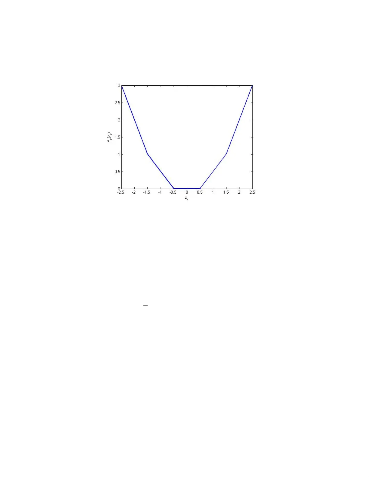
Co ordination of passiv e systems under quan tized measuremen ts ∗ Claudio De P ersis † Ba yu Ja y a wardhana ‡ Octob er 6, 2018 Abstract In this pap er w e in vestigate a passivit y approach to collectiv e co- ordination and sync hronization problems in the presence of quantized measuremen ts and show that coordination tasks can be ac hieved in a practical sense for a large class of passiv e systems. 1 In tro duction In the v ery activ e area of consensus, sync hronization and coordinated control there has b een an increasing in terest in the use of quan tized measurements and con trol ([28, 31, 24, 8, 29, 11] and references therein). As a matter of fact, since these problems in vestigate systems or agen ts whic h are distributed o v er a netw ork, it is very lik ely that the agen ts must exc hange information o v er a digital comm unication c hannel and quantization is one of the basic ∗ An abridged version of this pap er has b een presented at the 50th IEEE Conference on Decision and Con trol and European Con trol Conference, December 12-15, 2011, Or- lando, FL. This work is partially supported b y the Dutc h Organization for Scientific Re- searc h (NW O) within the pro ject QUantize d Information Contr ol for formation Ke eping (QUICK). † ITM, F acult y of Mathematics and Natural Sciences, Univ ersity of Groningen, the Netherlands, T el: +31 50 363 3080, Email: c.de.persis@rug.nl , and Dipartimen to di Informatica e Sistemistica, Sapienza Universit` a di Roma, Via Ariosto 25, 00185 Roma, Italy . ‡ ITM, F acult y of Mathematics and Natural Sciences, Univ ersity of Groningen, the Netherlands, T el: +31 50 363 7156, Email: bayujw@ieee.org, b.jayawardhana@rug.nl 1 limitations induced by finite bandwidth c hannels. T o cop e with this lim- itation, measuremen ts are processed by quan tizers, i.e. discon tinuous maps taking v alues in a discrete or finite set. Another reason to consider quantized measuremen ts stems from the use of coarse sensors. The use of quan tized measurements induces a partition of the space of mea- suremen ts: whenev er the measurement function crosses the boundary b e- t w een t wo adjacen t sets of the partition, a new v alue is broadcast through the c hannel. As a consequence, when the netw orked system under consideration ev olv es in contin uous time, as it is often the case with e.g. problems of co or- dinated motion, the use of quantized measuremen ts results in a completely async hronous exchange of information among the agents of the netw ork. De- spite the async hronous information exchange and the use of a discrete set of information v alues, meaningful examples of synchronization or coordination can b e obtained ([20, 13, 30, 18]). There are other approac hes to reac h synchronization (consensus) with an async hronous exchange of information, such as gossiping ([7, 9]), where at eac h time step tw o randomly c hosen agen ts exc hange information. The lat- ter approac h is conceptually v ery different from the one considered in this pap er, where the agents broadcast information when a lo cal even t o ccurs (the measuremen t crosses the partition b oundary). Moreo v er, while gossip- ing algorithms are mainly devised for discrete-time systems, here we focus on contin uous-time systems. In view of the sev eral contributions to quantized co ordination problems a v ailable for discrete-time systems ([28, 31, 24, 8, 29, 11]), one ma y won- der whether it would b e more con venien t simply to deriv e the sampled-data mo del of the system and then apply the discrete-time results. Due to the distributed nature of the system, a sampled-data approac h to the design of co ordinated motion algorithms presents a few dra wbacks: it might require sync hronous sampling at all the no des of the net work and consequen t accu- rate sync hronization of all the no de clocks; it migh t also require fast sampling rates, which ma y not b e feasible in a net work ed system with a large num b er of no des and connections. Finally , the sampled-data mo del ma y not fully preserv e some of the features of the original mo del. F or these reasons, we fo cus here on contin uous-time co ordination problems under quantized mea- suremen ts. A few works on this class of problems ha v e recen tly app eared. The work [18] deals with consensus algorithms using binary con trol algorithms. In [20] the atten tion is turned to quantized measurements and the consensus problem 2 under quan tized r elative measurements is tac kled. The same problem, but considering quan tized absolute measuremen ts, is studied in [13]. The pap er also in tro duces h ysteretic quantizers to prev ent the o ccurrence of c hattering due to the presence of sliding mo des. More recen tly , the work [30] has stud- ied the quan tized consensus algorithm for double in tegrators. A remark able adv ancemen t in the study of consensus algorithms o v er time-varying com- m unication graphs and using quantized measuremen ts has b een provided b y [23]. Despite the unquestionable in terest of the results in pap ers suc h as ([20, 13, 30, 18, 23]), they presen t an important limitation: they fo cus on agents with simple dynamics such as single ([20, 13, 18, 23]) or double in tegrators ([30]). The goal of this pap er is to inv estigate the p otentials of an approach to coordinated motion and sync hronization whic h tak es in to accoun t sim ul- taneously complex dynamics for the agen ts of the netw ork and quantized measuremen ts. In co ordinated motion, v ariables of interest are the p osition and the velocity of eac h subsystem, and the problem is to devise con trol la ws whic h guaran tee prescrib ed in ter-agen t p ositions and v elo cit y tracking. In this pap er we focus on the approach to co ordinated motion prop osed in [1]. In that paper, the author has sho wn ho w a n umber of co ordination tasks could be ac hieved for a class of passiv e nonlinear systems and has b een using this approac h for related problems in subsequen t w ork ([5, 6]). Others ha ve b een exploiting passivit y ([14, 26, 42, 32] to name a few) in connection with co ordination problems. Our interest for the approach in [1] stems from the fact that it allows to deal with complex co ordination tasks, including consensus with v elo cit y tracking, in wa y that naturally lends itself to deal with the presence of quan tized mea- suremen ts. In the approach of [1], a con tinuous feedback law is designed to ac hiev e the desired co ordination task under appropriate conditions. Th us the presence of quantized measuremen ts can b e tak en in to account in this setting by in tro ducing in the feedback law static discontin uous maps (the previously recalled quan tizers). Although in the case of quan tized measure- men ts the conditions in [1] are not fulfilled due to the discontin uous nature of the quan tizers, one can argue that an approximate or “practical” ([13]) co ordination task is ac hiev able under suitably mo dified conditions. This is the idea which is pursued in this pap er. In the case of a control system with a single commu nication c hannel this w as studied in [12]. Another reason to consider the approach of [1] is that it pro vides a systematic wa y to deal with a large v ariet y of co op erativ e con trol problems, as it has b een authoritativ ely 3 pro v en in the recent b o ok [3]. A second aim of this pap er is to study practical state sync hronization under quan tized output feedback. In these problems, one in vestigates conditions under whic h the state v ariables of all the subsystems asymptotically con- v erge to each other, with no additional requiremen t on the velocity tracking. P assivit y ([14, 39, 38]), or the weak er notion of semi-passivit y ([36, 35, 40]), has also pla yed an important role in synchronization problems. Here we mainly fo cus on the models considered in [14, 38]. The main contribution of this pap er is to sho w that some of the results of [1] and [38] hold in a practical sense in the presence of quantized measuremen ts. Because the latter introduces discon tinuities in the system, a rigorous analy- sis is carried out relying on notions and to ols from nonsmo oth control theory and differential inclusions. As far as the coordination problem is concerned, although the passivity approach of [1] allo ws to consider a large v ariety of co ordination con trol problems, in this paper we mainly focus on agreement problems in which agents aim at conv erging to the same p osition. A few other papers hav e app eared whic h deal with coordination problems for passiv e systems in the presence of quantization. The w ork [26] deals with a p osition co ordination problem for Lagrangian systems when dela ys and lim- ited data rates are affecting the system. The paper [22] deals with master- sla v e synchronization of passifiable Lurie systems when the master and the sla v e comm unicate o ver a limited data rate channel. The main difference of our pap er compared with [26, 22] is that in the former eac h system in the net w ork transmits quantized information in a completely asynchronous fash- ion and no common sampling time is required. F rom a mathematical point of view, this means that our approac h yields a discon tin uous closed-lo op system as opp osed to a sampled-data one. Moreov er, the classes of systems and the co ordination problems considered here app ear to b e different from those in [26, 22]. The organization of the pap er is as follows. The passivity approac h to co- ordination problems is recalled in Section 2. In Section 3 the co ordination con trol problem in the presence of uniform quan tizers is formulated and the main results are presen ted along with some examples. The sync hronization problem for passive systems under quantized output feedback is studied in Section 4. In Section 5 a few guidelines for future researc h are discussed. In the App endix some tec hnical to ols are reviewed for the sake of readers’ con v enience. 4 2 Preliminaries Consider N systems connected ov er an undirected graph G = ( V , E ), where V is a set of N no des and E ⊆ V × V is a set of M edges connecting the no des. The standing assumption throughout the pap er is that the graph G is c onne cte d . Eac h system i , with i = 1 , 2 , . . . , N , is asso ciated to the no de i of the graph and the edges connect the no des or systems whic h communicate. Eac h system i is describ ed by Σ i : ˙ ξ i = f i ( ξ i ) + g i ( ξ i ) u i w i = h i ( ξ i ) + v i , (1) where the state ξ i ∈ R n i , the input u i ∈ R p , the output w i ∈ R p , the exogenous signal v i ∈ R p and the maps f i , g i , h i are assumed to b e lo cally Lipsc hitz satisfying f i ( 0 ) = 0 , g i ( 0 ) full column-rank, h i ( 0 ) = 0 . F or the system Σ i , we assume the follo wing: Assumption 1 Ther e exists a c ontinuously differ entiable stor age function S i : R n i → R + which is p ositive definite and r adial ly unb ounde d such that ∇ S i ( ξ i )( f i ( ξ i ) + g i ( ξ i ) u i ) ≤ − W i ( ξ i ) + h i ( ξ i ) T u i , (2) wher e W i is a c ontinous p ositive function which is zer o at the origin. Suc h a system Σ i is called a strictly-passiv e system (with v i = 0). If W i is a non-negativ efunction, then Σ i is called a passive system. Lab el one end of eac h edge in E by a p ositiv e sign and the other one by a negativ e sign. No w, consider the k -th edge in E , with k ∈ { 1 , 2 , . . . , M } , and let i, j b e the tw o no des connected b y the edge. F or the coordination problem, whic h is detailed in Subsection 2.1, the relativ e measurements of the in tegral form R t 0 w i ( τ )d τ and R t 0 w j ( τ )d τ are used. On the other hand, for the synchronization problem, whic h is briefly reviewed in Subsection 2.2, w e need the relativ e measuremen ts of the signals w i and w j . Th us, dep ending up on sp ecific problems, let z k describ e the difference betw een the signals w i and w j (or the difference b et w een the signals x i ( t ) := R t 0 w i ( τ )d τ + x i (0) and x j ( t ) := R t 0 w j ( τ )d τ + x j (0) with constan t v ectors x i (0) , x j (0) ∈ R p ) and be defined as follows: z k =  w i − w j (or x i − x j ) if i is the p ositiv e end of the edge k w j − w i (or x j − x i ) if i is the negative end of the edge k . 5 Recall also that the incidence matrix D asso ciated with the graph G is the N × M matrix suc h that d ik =    +1 if no de i is the p ositiv e end of edge k − 1 if no de i is the negative end of edge k 0 otherwise . By the definition of D , the v ariables z can b e concisely represented as z = ( D T ⊗ I p ) w  or z = ( D T ⊗ I p ) x  (3) where w = [ w T 1 . . . w T N ] T and x = [ x T 1 . . . x T N ] T , resp ectiv ely , and the sym b ol ⊗ denotes the Kronec ker product of matrices (see App endix A for a definition). In this pap er w e are interested in con trol laws which use quantized measure- men ts. F or eac h k = 1 , 2 , . . . , M , instead of z k , the vector q ( z k ) := ( q ( z k 1 ) . . . q ( z kp )) T is a v ailable, where q is the quantizer map which is defined as follows. Giv en a p ositiv e real num b er ∆, we let q : R → Z ∆ b e the function q ( r ) = ∆  r ∆ + 1 2  (4) with 1 ∆ the precision of the quantizer. As ∆ → 0, q ( r ) → r . Observe that eac h en try of z k is quantized indep endently of the others and the quan tized information is then used in the con trol law. Remark 1 The results of the pap er con tin ue to hold if each quan tizer has its o wn resolution (that is, the information z kj is quan tized by a quan tizer with resolution ∆ kj ). How ever, to reduce the notational burden, w e only deal with the case in whic h the quan tizers hav e all the same resolution ∆. In the follo wing subsections, we review the results on passivity approac h to the co ordination problems of [1] and to the synchronization problems of [38] without the quantized measuremen ts. 6 2.1 P assivit y approach to the co ordination problem In the co ordination problems of [1], the signal w i of eac h system Σ i corre- sp onds to the velocity of the system, and thus, x i , i = 1 , . . . , N , represen ts the p ositions whic h must b e coordinated (recall that x i ( t ) := R t 0 w i ( τ )d τ + x i (0)). The co ordination problem under consideration requires all the systems of the formation to mo ve with a prescrib ed velocity v , i.e., v 1 = v 2 = . . . = v N = v . Define y i = ˙ x i − v (5) the v elo cit y tracking error. It can b e chec ked from (1) and the definition of ˙ x i that y i = h ( ξ i ). The standing assumption is that, p ossibly after a preliminary feedback whic h uses information av ailable lo cally , eac h system Σ i is strictly passive, i.e., (2) holds with W i p ositiv e definite. In other w ords, it is strictly passive from the control input u i to the velocity error y i . F or the sake of conciseness, the equations (1), (5) are rewritten as ˙ x =    h 1 ( ξ 1 ) . . . h N ( ξ N )    | {z } h ( ξ ) +    v . . . v    | {z } 1 N ⊗ v ˙ ξ =    f 1 ( ξ 1 ) . . . f N ( ξ N )    | {z } f ( ξ ) +    g 1 ( ξ 1 ) . . . 0 . . . . . . . . . 0 . . . g N ( ξ N )    | {z } g ( ξ ) u (6) where x = ( x T 1 . . . x T N ) T , ξ = [ ξ T 1 . . . ξ T N ] T , u = [ u T 1 . . . u T N ] T , 1 N is the N - dimensional v ector whose en tries are all equal to 1 and 0 denotes a v ector of appropriate dimension of all zeros. The formation control problem consists of designing eac h con trol law u i , with i = 1 , 2 , . . . , N , in such a w ay that it uses only the information a v ailable to the agent i and guarantees the following tw o specifications: (i) lim t →∞ | ˙ x i ( t ) − v ( t ) | = 0 for eac h i = 1 , 2 , . . . , N , with v ( t ) a b ounded and piece-wise contin uous reference v elo city for the formation; (ii) z k ( t ) → A k as t → ∞ for eac h k = 1 , 2 , . . . , M , where A k ⊂ R p are the prescrib ed sets of conv ergence 1 and z = ( D T ⊗ I p ) x as defined in (3). 1 W e refer the interested reader to [1] for examples of sets A k related to some co ordi- 7 In [1], where measurements without quan tization are considered, the case A k = { 0 } is referred to as the agr e ement pr oblem . Let P k : R p → R , for k = 1 , 2 , . . . , N , b e nonnegativ e con tin uously dif- feren tiable (the latter assumption will b e remo ved in the next section) and radially unbounded functions whose minimum is ac hiev ed at the p oin ts in A k . T o be more precise, the functions P k are assumed to satisfy P k ( z k ) = 0 and ∇ P k ( z k ) = 0 if and only if z k ∈ A k . (7) Define ∇ P k ( z k ) = ψ k ( z k ) . (8) The feedbac k laws proposed in [1] to solv e the problem form ulated ab o ve are: u i = − M X k =1 d ik ψ k ( z k ) , i = 1 , 2 , . . . , N . (9) Observ e that, as required, eac h con trol la w u i uses only information which is a v ailable to the agent i . Indeed, d ik 6 = 0 if and only if the edge k connects i to one of its neigh b ors. In compact form, (9) can b e rewritten as u = − ( D ⊗ I p ) ψ ( z ) , (10) where ψ ( z ) = [ ψ 1 ( z 1 ) T . . . ψ M ( z M ) T ] T and z is as in (3). Before ending the section, w e recall that the system b elo w with input ˙ x and output − u , namely (see Figure 2 in [1] for a pictorial representation of the system) ˙ z = ( D T ⊗ I p ) ˙ x − u = ( D ⊗ I p ) ψ ( z ) (11) is passive from ˙ x to − u with storage function P M k =1 P k ( z k ). W e remark that the function P k ( z k ) is c hosen in suc h a w ay that the region where the v ariable z k m ust conv erge for the system to achiev e the prescrib ed co ordination task coincides with the set of the global minima of P k ( z k ). Hence, the co ordination task guides the design of P k ( z k ) whic h in turn allo ws to determine the con trol functions (9) via (8). The functions P k ( z k ) in the case of agreemen t problems via quantized control laws will b e designed in Section 3. nation problems. The sets A k whic h are of in terest in this paper will b e in tro duced in (16). 8 2.2 P assivit y approach to the sync hronization problem In the sync hronization problem of [38, Theorem 4], eac h system Σ i in (1) (with v i = 0) is assumed to b e linear, identical and passiv e. F or suc h setting, eac h (passive) system Σ i is of the form ˙ ξ i = Aξ i + B u i w i = C ξ i i = 1 , 2 , . . . , N (12) where ξ i ∈ R n , u i , w i ∈ R p and the passivity of Σ i implies that the following assumption holds: Assumption 2 Ther e exists an ( n × n ) matrix P = P T > 0 such that A T P + P A ≤ 0 , B T P = C . The synchronization problems can then b e stated as designing each con- trol la w u i , i = 1 , 2 , . . . , N , using only the information a v ailable to te agent i such that, for ev ery i , ξ i − ξ 0 → A where ξ 0 is the tra jectory of the au- tonomous system ˙ ξ 0 = Aξ 0 whic h is initialized b y the av erage of the initial states, i.e., ξ 0 (0) = 1 N P i ξ i (0), and A ⊂ R p is the prescrib ed set of con ver- gence. In the case without the quantized measuremen ts, which is treated in [38], A = { 0 } . The co ordination problem that is review ed in Subsection 2.1, is related to the case when ˙ ξ 0 = 0 [1]. F or another viewp oin t, we can consider that (12) corresp onds to the case in the Subsection 2.1, where the mapping u 7→ y is an iden tit y op erator, v = 0 and one takes into accoun t dynamics on the subsystem x whic h are more complex than those of a single in tegrator. In addition to output sync hronization, it is well-kno wn that the states of interconnected passive systems synchronize under observ ability assump- tion ([14]). The largest inv ariant set of the interconnected systems, when the measurements are not quantized and ( C , A ) is observ able, is the set { ξ ∈ R nN : ξ 1 = . . . = ξ N } . In the case of quan tized measurements, the in v arian t set is larger. Our main result in Section 4 pro vides an estimate of the inv ariant set of the interconnected systems with quan tized measure- men ts. T o this purp ose, w e rely on a result of exp onen tial synchronization under static output feedbac k con trol la ws and time-v arying graphs whic h has b een in v estigated in [38]. In the follo wing statement, we recall Theorem 4 of [38] sp ecialized to the case of time-inv ariant undirected graphs: 9 Theorem 1 L et Assumption 2 hold and supp ose that the p air ( C , A ) is ob- servable. L et the c ommunic ation gr aph b e undir e cte d and c onne cte d, and denote z = ( D T ⊗ I p ) w as in (3) with w = [ w T 1 . . . w T N ] T . Then the solutions of ˙ ξ i = Aξ i − B M X k =1 d ik z k , i = 1 , 2 , . . . , N (13) satisfy lim t → + ∞     ξ i ( t ) − 1 T N ⊗ I n N ξ ( t )     = 0 (14) wher e ξ = [ ξ T 1 ξ T 2 · · · ξ T N ] T and the c onver genc e is exp onential. Mor e pr e cisely, the solutions c onver ge exp onential ly to the solution of ˙ ξ 0 = Aξ 0 initialize d to the aver age of the initial c onditions of the systems (13) , i.e. ξ 0 (0) = 1 T N ⊗ I n ξ (0) / N . Let ˜ ξ = ξ − 1 N 1 T N ⊗ I n N ξ = (Π ⊗ I n ) ξ , with Π = I N − 1 N 1 T N N , b e the disagree- men t vector. F rom (13), ˜ ξ ( t ) obeys the equation ˙ ˜ ξ = [ I N ⊗ A − ( I N ⊗ B )( D D T ⊗ I p )( I N ⊗ C )] | {z } ˜ A ˜ ξ (15) and the conv ergence result (14) can b e restated as lim t → + ∞ || ˜ ξ ( t ) || = 0. The pro of of the result rests on showing that the Lyapuno v function V ( ˜ ξ ) = ˜ ξ T ( I N ⊗ P ) ˜ ξ along the solutions of (15) satisfies the inequality ˙ V ( ˜ ξ ) ≤ − λ 2 || (Π ⊗ I p ) ˜ ξ || 2 , where λ 2 is the algebraic connectivity of the graph, i.e. the smallest non-zero eigen v alue of the Laplacian L = D D T . Then the thesis descends from the observ abilit y assumption and Theorem 1.5.2 in [37]. 3 Quan tized co ordination con trol 3.1 A practical agreemen t problem Despite the generality allow ed b y the passivit y approach of [1], in this pap er w e fo cus on an agreemen t problem. By an agreemen t problem it is meant 10 a sp ecial case of co ordination in which all the v ariables x i connected by a path conv erge to eac h other. In the problem formulation in Section 2, this amoun ts to hav e A k = { 0 } for all k = 1 , 2 , . . . , M . When using static al ly 2 quan tized measuremen ts, how ever, it is a well established fact ([28, 20, 13]) that a co ordination algorithm leads to a practical agreemen t result, meaning that each v ariable z k con v erges to a compact set con tainingthe origin, rather than to the origin itself. Motiv ated by this observ ation, w e set in this paper a w eak er conv ergence goal, namely for each k = 1 , 2 , . . . , M , w e ask the target set A k to b e of the form: A k = p × j =1 [ − a, a ] (16) where a is a p ositiv e constant and the sym b ol × denotes the Cartesian pro d- uct. Then the design pro cedure of Section 2 prescribes to c ho ose a non- negativ e p oten tial function P k ( z k ) whic h is radially un b ounded on its domain of definition and suc h that (7) holds. If suc h a function exists then the con- trol law is chosen via (8). T o take in to accoun t the presence of quantized measuremen ts, the nonlinearities ψ k on the righ t-hand side of (8) should tak e the form ψ k ( z k ) = χ k ( q ( z k )) , (17) with χ k to b e defined later. The presence of quan tized measurements, i.e. of q ( z k ), makes the righ t-hand side of (8) discon tinuous and asks for a redefinition of the requiremen ts (7). In this paper, we lo ok for a lo c al ly Lipschitz radially un b ounded non-negativ e functions P k whic h satisfy P k ( z k ) = 0 and 0 ∈ ∂ P k ( z k ) if and only if z k ∈ A k , (18) where ∂ P k ( z k ) is the Clark e generalized gradien t (see Appendix B for a def- inition) whic h is needed since P k ( z k ) is no w not con tin uously differen tiable. Similarly to (7), w e are asking A k to b e the set of all local and global minima for P k ( z k ). A candidate function P k ( z k ) with the prop erties (18) and suc h that a function χ k exists for which (8), (17) hold, is the function P k ( z k ) = p X j =1 Z z kj 0 q ( s ) ds, (19) 2 The use of dynamic quantizers can lead to asymptotic results. See [10, 29] for a few results for discrete-time systems. Dealing with con tinuous-time systems and dynamic quan tizers p oses a few extra challenges, which are not addressed in this pap er. 11 Figure 1: The graph of P k ( z k ) with z k ∈ R and ∆ = 1. where z kj is the j th comp onent of the vector z k ∈ R p (see Fig. 1 for a picture of P k ( z k )). Suc h a function is defined on all R p , is radially un b ounded and lo cally Lipsc hitz. By Rademacher’s theorem ([17], Chapter 3) it is differentiable almost ev erywhere. In all the p oin ts of R p where it is differentiable ∇ P k ( z k ) = q ( z k ) i.e. (8), (17) holds with χ k = Id (Id : R p → R p is the identit y function). Bearing in mind the definitions (4) and (16), to satisfy (18) it is necessary and sufficient to set a = ∆ 2 . In what follows we examine the ev olution of the system (6) under the con trol law: u i = − M X k =1 d ik q ( z k ) , i = 1 , 2 , . . . , N . (20) 3.2 Closed-lo op system Similarly to (10), we write the quantized control law in compact form as: u = − ( D ⊗ I p ) q ( z ) , (21) 12 where q ( z ) = ( q ( z 1 ) T . . . q ( z M ) T ) T . The closed-lo op system then takes the follo wing expression: ˙ x = h ( ξ ) + 1 N ⊗ v ˙ ξ = f ( ξ ) + g ( ξ )( − ( D ⊗ I p ) q ( z )) , (22) where z = ( D T ⊗ I p ) x and the maps f , g , h are as in (6). 3.2.1 Con trol scenario and implementation Before pro ceeding to the analysis of the system, it is important to motiv ate in more detail the con trol scenario w e consider and ho w the o v erall control sc heme is implemented. F or each pair of neighboring agents, one of the tw o is equipp ed with a sensor whic h contin uously take the relativ e measurement with resp ect to its neigh- b or, e.g., a sonar or a radar. Not all the agen ts are equipp ed with these sensors since they migh t ha v e v ery dedicated tasks in the formation and space m ust b e sav ed for other hardware needed to accomplish these tasks. On the other hand, since these agen ts need information to main tain their p ositions in the formation, they receive such information in quantized form from their neighbors via a digital comm unication channel. The implemen tation of the con trol law in (22) can b e giv en b y the quantization- b ase d distribute d c ontr ol pr oto c ol as follows. ( Initialization .) A t time t 0 = 0, all sensors measures z k ( t 0 ), k = 1 , 2 , . . . , p . The pro cessing units collo cated with the sensors computes q ( z k ( t 0 )) and the resulting v alue is broadcasted to its neigh b ors. Each agent i computes the lo cal control la w u i as in (20) and the control v alue is held until new in- formation is av ailable. Note that the closed-lo op system evolv es according to ˙ x = h ( ξ ) + 1 N ⊗ v ˙ ξ = f ( ξ ) + g ( ξ )( − ( D ⊗ I p ) q ( z ( t 0 ))) for all t > t 0 un til new information is av ailable. ( Quantization-b ase d tr ansmission and c ontr ol up date .) Let ` = 1 and let t ` b e the smallest time at which t ` > t ` − 1 and the pro cessing unit of a sensor in the k -th edge detects that q ( z k ( t ` )) 6 = q ( z k ( t ` − 1 )). In this case, the quantized information q ( z k ( t ` )) is transmitted to its neighbor and the lo cal con trol law of the i -th and j -th agents, where ( i, j ) is the pair of no des linked by the 13 k -th edge, is updated by u i ( t ` ) = u i ( t ` − 1 ) − d ik  q ( z k ( t ` )) − q ( z k ( t ` − 1 ))  u j ( t ` ) = u j ( t ` − 1 ) − d j k  q ( z k ( t ` )) − q ( z k ( t ` − 1 ))  . There is no other information exc hange and hence the rest of the agen ts main tains their lo cal con trol v alues. The lo cal control law is now fixed until new information is transmitted again. F or all t > t ` and until this new transmission o ccurs, the evolution of the closed-lo op system is giv en by ˙ x = h ( ξ ) + 1 N ⊗ v ˙ ξ = f ( ξ ) + g ( ξ )( − ( D ⊗ I p ) q ( z ( t ` ))) . The quan tization-based even t-triggered control up date pro cess is iterated with the index v alue ` incremented by one. A few remarks are in order: (i) The construction outlined ab o ve results in a sequence of unev enly-spaced sampling times t ` , ` ∈ N , at which sensors located at the systems broad- cast quan tized information to neigh b oring systems. This information is used b y lo cal controllers to up date the control v alue. The control la ws turn out to b e piece-wise constan t functions of time whose v alue is up dated whenever new information is received. (ii) Notice that ev en the agent which measures z k implemen ts a control law in which q ( z k ) is used instead of z k itself. This is mainly motiv ated by our need to preserve a “symmetric” structure in the closed-loop system. In fact, giv en agen ts i, j and their relative distance z k , in the case of unquan tized information, agen t i would use z k in the con trol law, and agen t j , − z k . Similarly , in the case of quan tized measurements, it is v ery helpful in the analysis to emplo y q ( z k ) in the con trol law for agen t i and − q ( z k ) in the one for agent j . (iii) In the quantization-based transmission and control proto col described ab o v e, the solution of the closed-lo op system is not prev ented to ev olv e along a discon tinuit y surface. In practice, due to dela ys in the transmis- sion and in the implemen tation of the control law, this could result in c hattering, which is of course undesirable in the present context, since it w ould require fast information transmission. Nevertheless, in [13] a new class of hybrid quantizers hav e b een considered whic h preven t the 14 o ccurrence of chattering. This class could also b e used for the problem at hand in this pap er, but this is not pursued further for the sak e of brevit y . 3.2.2 A notion of solution The system (22) has a discon tinuous righ t-hand side due to the presence of the quan tization functions and its analysis requires a suitable notion of solution. In this pap er w e adopt Krasowskii solutions. In fact, it w as sho wn in [13] that Carath ´ eodory solutions ma y not exist for agreemen t problems. Moreov er, Kraso wskii solutions include Carath´ eo dory solutions and the results w e deriv e for the former also holds for the latter in case they exist. Denoted b y ˙ X ( t ) = F ( t, X ) the system (22), a function X ( · ) defined on an in terv al I ⊂ R is a Krasowskii solution to the system on I if it is absolutely con tin uous and satisfies the differential inclusion ([25]) ˙ X ( t ) ∈ K ( F ( t, X )) := \ δ > 0 co ( F ( t, B ( X , δ ))) (23) for almost every (a.e.) t ∈ I . The op erator co( S ) denotes the conv ex closure of S , i.e. the smallest closed set containing the conv ex h ull of S . Since the righ t-hand side of (22) is lo cally bounded, lo cal existence of Kraso wskii solutions is guaranteed ([25]). The differential inclusion corresp onding to the system (22) can b e written explicitly . More precisely , for every k ∈ { 1 , 2 , . . . , M } and i ∈ { 1 , 2 , . . . , p } , w e observe that K q ( r ) is given by K q ( r ) =  m ∆ r ∈  ( m − 1 2 )∆ , ( m + 1 2 )∆  , m ∈ Z [ m ∆ , ( m + 1)∆] r = ( m + 1 2 )∆ , m ∈ Z . Using K q , the differen tial inclusion (23) for (22) can b e written as ˙ x = h ( ξ ) + 1 N ⊗ v ˙ ξ ∈ f ( ξ ) + g ( ξ )( − ( D ⊗ I p ) K q ( z )) , (24) where K q ( z ) := × M k =1 K q ( z k ), K q ( z k ) := × p j =1 K q ( z kj ). Note that we hav e used the calculus rule for the set-v alued map K K  g ( ξ )( − ( D ⊗ I p ) q ( z ))  = g ( ξ )( − ( D ⊗ I p ) K q ( z )) 15 (see also [19, 34, Theorem 1]). The Krasowskii solutions to (22) are also Filipp o v solutions as it follo ws from [25, Lemma 2.8] for a piecewise con- tin uous v ector field F . Since ev ery Carath´ eo dory solutions to (22) is also a Kraso wskii solution to (22), the stability prop erties of the Krasowskii solu- tions are also inherited b y the classical Carath´ eo dory solutions [25] in case the latter exist. 3.2.3 Analysis Recalling that ( D T ⊗ I p )( 1 N ⊗ v ) = 0 and b earing in mind (11), the system (22) in the co ordinates ( z , ξ ) writes as ˙ z = ( D T ⊗ I p ) h ( ξ ) ˙ ξ = f ( ξ ) + g ( ξ )( − ( D ⊗ I p ) q ( z )) . (25) Ev en the system ab o ve is discon tinuous and again its solutions must be in- tended in the Krasowskii sense. It is straigh tforward to v erify that, given an y Kraso wskii solution ( x, ξ ) to (22), the function ( z , ξ ) = (( D T ⊗ I p ) x, ξ ) is a Kraso wskii solution to (25). The differential inclusion corresp onding to (25) is easily understoo d from (24). In what follo ws w e in v estigate the asymptotic prop erties of the Kraso wskii solutions to (25) and infer stability prop erties of (22). A few notions of nonsmo oth control theory whic h are used in the pro ofs are recalled in the App endix B. The first fact we notice is the follo wing: Lemma 1 L et Assumption 1 hold and let the c ommunic ation gr aph G b e undir e cte d and c onne cte d. Then any Kr asowskii solution to (25) c onver ges to the set of Kr asowskii e quilibria: { ( z , ξ ) : ξ = 0 , 0 ∈ ( D ⊗ I p ) K q ( z ) } . (26) Pr o of: T o analyze the system (25) we consider the Lyapuno v function V ( z , ξ ) = N X i =1 S i ( ξ i ) | {z } S ( ξ ) + M X k =1 P k ( z k ) | {z } P ( z ) = P N i =1 S i ( ξ i ) + M X k =1 p X j =1 Z z kj 0 q ( s ) ds . 16 The function is a lo cally Lipsc hitz and regular function. In fact, each term R z kj 0 q ( s ) ds is con vex and as suc h it is regular ([16, Prop osition 2.3.6],[19]). Then the sums P k ( z k ) and P M k =1 P k ( z k ) are also regular. The function V ( z , ξ ) is nonnegativ e and v anishes on the set of p oin ts such that ξ = 0 and z kj ∈ [ − a, a ] for all k ∈ { 1 , 2 , . . . , M } and all j ∈ { 1 , 2 , . . . , p } . In order to apply the LaSalle’s inv ariance principle for the differen tial in- clusions as given in Theorem 4 in App endix B, w e analyze the set-v alued deriv ativ e V with resp ect to (25) as follo ws. Define ˙ V ( z , ξ ) = { a ∈ R : ∃ w ∈ K ˜ F ( z , ξ ) s . t . a = h p, w i , ∀ p ∈ ∂ V ( z , ξ ) } . where h· , ·i denotes the standard inner pro duct and ˜ F ( z , ξ ) the righ t-hand side of (25). W e first observ e that b y definition of V ( z , ξ ), ∂ V ( z , ξ ) and ∂ P ( z ), p ∈ ∂ V ( z , ξ ) implies the existence of p z ∈ ∂ P ( z ) such that p =  p z ∇ S ( ξ )  . Moreo v er, if w ∈ K ˜ F ( z , ξ ) then there exists w z ∈ K q ( z ) ([25],[34]) such that w =  ( D T ⊗ I p ) h ( ξ ) f ( ξ )  +  0 g ( ξ )  ( − D ⊗ I p ) w z . Let now p ∈ ∂ V ( z , ξ ) and w ∈ K ˜ F ( z , ξ ) and write h p, w i = h∇ S ( ξ ) , f ( ξ ) + g ( ξ )( − D ⊗ I p ) w z i + h p z , ( D T ⊗ I p ) h ( ξ ) i ≤ − N X i =1 W i ( ξ i ) + h h ( ξ ) , ( − D ⊗ I p ) w z i + h p z , ( D T ⊗ I p ) h ( ξ ) i , (27) where the inequalit y is a consequence of (2). Supp ose now that for some ( z , ξ ), ˙ V ( z , ξ ) 6 = ∅ . Then, for ev ery a ∈ ˙ V ( z , ξ ) and for ev ery p ∈ ∂ V ( z , ξ ), there exists w ∈ K ˜ F ( z , ξ ) such that a = h p, w i . By definition of q ( z ) and P ( z ), ∂ P ( z ) = K q ( z ) ([25],[34]). Then a = h p, w i holds in particular when p =  p z ∇ S ( ξ )  =  w z ∇ S ( ξ )  . 17 with w z ∈ K q ( z ). Then (27) b ecomes: h p, w i ≤ − N X i =1 W i ( ξ i ) + h h ( ξ ) , ( − D ⊗ I p ) w z i + h w z , ( D T ⊗ I p ) h ( ξ ) i = − N X i =1 W i ( ξ i ) . Hence, for all ( z , ξ ) suc h that ˙ V ( z , ξ ) 6 = ∅ , w e hav e that ˙ V ( z , ξ ) = { a ∈ R : a ≤ − N X i =1 W i ( ξ i ) } . (28) Since d dt V ( z ( t ) , ξ ( t )) ∈ ˙ V ( ξ ( t ) , z ( t )) ⊆ ( −∞ , 0] for almost ev ery t , V ( z ( t ) , ξ ( t )) cannot increase, and an y Krasowskii solution ( z ( t ) , ξ ( t )) is b ounded. Hence, ( z ( t ) , ξ ( t )) exists for all t . Giv en an y initial condition ( z (0) , ξ (0)), the set S such that V ( z , ξ ) ≤ V ( z (0) , ξ (0)) is a strongly inv ariant set for (25) whic h con tains the initial condi- tion. An application of Theorem 4 in App endix B shows that an y Kra- so wskii solution conv erges to the largest weakly inv ariant set contained in S ∩ { ( z , ξ ) : 0 ∈ ˙ V ( z , ξ ) } . Moreo v er, in view of (28), the set Z of p oin ts ( z , ξ ) suc h that 0 ∈ ˙ V ( z , ξ ) is con tained in the set of p oints such that ξ = 0 . Hence, an y p oin t of the largest weakly inv ariant set con tained in S ∩ Z is such that ξ = 0 . Pic k a p oin t ( z , 0 ) on this in v ariant set. Then in order for a Kraso wskii solution to (25) starting from this p oin t to remain in the in v ariant set, it m ust b e true that 0 ∈ f ( 0 ) + g ( 0 )( − ( D ⊗ I p ) K q ( z )) = g ( 0 )( − ( D ⊗ I p ) K q ( z )). Since the matrix g ( 0 ) is full-column-rank (recall that eac h g i ( 0 ) is full-column rank), the in- clusion ab o v e requires the existence of w z ∈ K q ( z ) such that ( D ⊗ I p ) w z = 0 . In other w ords, the largest w eakly in v ariant set included in S ∩ Z is con tained in the set (26). Finally , observe that, tak en an y point in the set (26) as initial condition for (25), at least a Krasowskii solution ( z ( t ) , ξ ( t )) originating from this p oin t must coincide with the trivial solution, i.e. ( z ( t ) , ξ ( t )) = ( 0 , 0 ) for all t . Hence, an y p oint in (26) is a Kraso wskii equilibrium for (25). It is now p ossible to pro ve the following: 18 Theorem 2 L et Assumption 1 hold and let the c ommunic ation gr aph G b e undir e cte d and c onne cte d. L et v : R + → R p b e a b ounde d and pie c ewise c on- tinuous function and ∆ b e a p ositive numb er. Then any Kr asowskii solution to (22) c onver ges to the set { ( x, ξ ) : ξ = 0 , z ∈ ( A 1 × . . . × A M ) , z = ( D T ⊗ I p ) x } , (29) wher e the sets A k ’s ar e define d in (16), with a = ∆ / 2 . Mor e over, lim t → + ∞ [ ˙ x ( t ) − 1 N ⊗ v ( t )] = 0 . Pr o of: Consider an y Kraso wskii solution ( x ( t ) , ξ ( t )) to (22), whose existence is guaran teed lo cally . It can also b e extended for all t ∈ [0 , + ∞ ). In fact supp ose by contradiction this is not true, i.e. ( x ( t ) , ξ ( t )) is defined on the in terv al [0 , t f ), with t f < + ∞ . Define ( z ( t ) , ξ ( t )) = (( D T ⊗ I p ) x ( t ) , ξ ( t )). ( z ( t ) , ξ ( t )) is a Krasowskii solution to (25). As pro v en b efore, such a solution is b ounded on its its domain of definition. Since by (22) ˙ x ( t ) = h ( ξ ( t )) + v ( t ) and b oth the terms on the righ t-hand side are b ounded, then x ( t ) grows linearly in t and therefore it must b e b ounded on the maximal in terv al of definition, i.e. t f = + ∞ . Hence both ( x ( t ) , ξ ( t )) and ( z ( t ) , ξ ( t )) = (( D T ⊗ I p ) x ( t ) , ξ ( t )) are defined for all t . Moreov er, b y Lemma 1, z ( t ) = ( D T ⊗ I p ) x ( t ) con v erges to the set of points (26), i.e. to { ( x, ξ ) : ξ = 0 , 0 ∈ ( D ⊗ I p ) K q ( z ) , z = ( D T ⊗ I p ) x } . (30) Let ( x, 0 ) b elong to the set (30). Then z = ( D T ⊗ I p ) x , i.e. z b elongs to the span of D T ⊗ I p and there exists w z ∈ K q ( z ) such that ( D ⊗ I p ) w z = 0 . The t wo conditions imply that h w z , z i = 0. W e claim that then necessarily z ∈ A 1 × . . . × A M , with the sets A i ’s given in (16). In fact, if this is not true, then there m ust exist a pair of indices j, k suc h that | z kj | > a . This implies that the entry k + j of the v ector w z is differen t from zero and also w z ,k + j · z kj > 0. Moreov er, since w z ∈ K q ( z ), for any pair of indices i, ` such that i 6 = k or ` 6 = j , w z ,i + ` · z i` ≥ 0. This contradicts that h w z , z i = 0. Then w e hav e prov en that the set (30) is included in the set { ( x, ξ ) : ξ = 0 , z ∈ A 1 × . . . × A M , z = ( D T ⊗ I p ) x } . (31) Hence, an y Krasowskii solution ( x ( t ) , ξ ( t )) to (22) con verges to a subset of (31). As for the second part of the statement, an y Krasowskii solution to (22) is suc h that ˙ x ( t ) − 1 N ⊗ v ( t ) = h ( ξ ( t )), and since we ha v e pro v en that ξ ( t ) → 0 as t → ∞ , we hav e also prov en that lim t → + ∞ [ ˙ x ( t ) − 1 N ⊗ v ( t )] = 0 . 19 3.3 Examples W e provide three examples of application of the quan tized agreemen t result describ ed ab o v e. A gr e ement of single inte gr ators by quantize d me asur ements. W e specialize the pro of of Theorem 2 to the agreemen t problem for single in tegrators. This problem stems from the case when in (22) the mapping from u = − ( D ⊗ I p ) q ( z ) to y = h ( ξ ) is an identit y op erator. The closed-lo op system (22) reduces to: ˙ x = − ( D ⊗ I p ) q ( z ) z = ( D T ⊗ I p ) x (32) whic h using the v ariables z b ecomes ˙ z = − ( D T ⊗ I p )( D ⊗ I p ) q ( z ) = − ( D T D ⊗ I p ) q ( z ) (33) W e analyze this system using the function P ( z ) introduced ab ov e. Since ∂ P ( z ) = K q ( z ), then for all z suc h that ˙ P ( z ) 6 = ∅ , we ha v e ˙ P ( z ) = { a ∈ R : ∃ w z ∈ K q ( z ) s . t . a = −|| ( D ⊗ I p ) w z || 2 } . Hence, arguments as in Lemma 1 give that all the Kraso wskii solutions to (33) conv erge to the set of p oints { z : 0 ∈ ( D ⊗ I p ) K q ( z ) } . On the other hand, by Theorem 2, any Kraso wskii solution x ( t ) to (32) is suc h that z ( t ) = ( D T ⊗ I p ) x ( t ) con v erges to { x : 0 ∈ ( D ⊗ I p ) K q ( z ) , z = ( D T ⊗ I p ) x } whic h is included in the set { z : z ∈ A 1 × . . . × A p , z = ( D T ⊗ I p ) x } . Let x b e an y Krasowskii solution to (32) with z = ( D T ⊗ I p ) x . T ake an y t w o v ariables x i , x j whose agents are connected by the edge k . Consider for the sake of simplicit y that each quan tizer has the same parameter ∆. Then z k = x i − x j con v erges asymptotically to a square of the origin whose edge is not longer than ∆. If the agents are not connected b y an edge but b y a path, then eac h en try of x i − x j is in magnitude bounded b y ∆ · d , with d the diameter of the graph. The result can b e compared with Theorem 4 in [20]. One difference is that, while trees are considered in [20], connected graphs are considered here. Moreov er, in [20] the scalar states are guaran teed to con v erge to a ball of radius || D T D || √ M λ min ( D T D ) ∆. Hence, denoted b y ρ the ratio || D T D || λ min ( D T D ) and considered the b ound M ≤ N − 1, an y t w o states x i , x j ma y differ for 2 ρ ∆ √ N − 1. The passivity approach considered here yields that they differ for not more than d · ∆, where d gro ws as O ( ρ log ( N )) ([15]) 20 for not complete and regular graphs (graphs with all the no des having the same degree), th us leading to a smaller region of conv ergence, the quan tizer resolution ∆ b eing the same. A gr e ement of double inte gr ators by quantize d me asur ements Consider the case of N agen ts mo deled as ¨ x i = f i , i = 1 , 2 , . . . , N , (34) with x i , f i ∈ R 2 , for which w e wan t to solv e the agreemen t problem with quan tized measuremen ts. This means that all the agents should practically con v erge tow ards the same p osition and also asymptotically evolv e with the same velocity v . The preliminary feedback ([1]) f i = − K i ( ˙ x i − v ) + ˙ v + u i , K i = K T i , (35) with u i to design, and the change of v ariables ξ i = ˙ x i − v , makes the closed- lo op system ˙ x i = ξ i + v ˙ ξ i = − K i ξ i + u i y i = ξ i passiv e with storage function S i ( ξ i ) = 1 2 ξ T i ξ i and W i ( ξ i ) = − K i ξ T i ξ i . The system ab ov e is in the form (1). Theorem 2 guaran tees that the Krasowskii solutions of (34), (35), (21) conv erges asymptotically to the set (29) and that all the agen ts’ v elo cities conv erge to v . In other w ords, the formation ac hiev es practical p osition agreement and conv ergence to the prescrib ed velocity . Remark 2 (Consensus for double integrators with velocity feedbac k) A different but related consensus problem consists of designing lo cal con- trollers in suc h a wa y that each double in tegrator con verges asymptotically to the same p osition and velocity . In this case, no external reference ve- lo cit y is provided and the v elo city to whic h all the systems conv erge is the a v erage of the initial velocities ([41]). The controller whic h guaran tees this co ordination task uses b oth p osition and velocity feedback (observe that the comm unication graphs for the p osition measuremen ts and for the velocity measuremen ts can b e different). It then makes sense to consider the problem in the presence of quan tized relative p osition and velocity measuremen ts. This has b een inv estigated in [30]. 21 The c ase of unknown r efer enc e velo city. If the reference v elo city v is not av ailable to all the agents, then [4, 6] suggest to replace it with an estimate which is generated by each agen t on the basis of the current av ailable measuremen ts. Here w e examine this con trol sc heme when the measuremen ts are quan tized. W e consider the sp ecial case in which the unknown reference v elo cit y is constant. Then each agen t i , with the exception of one whic h acts as a leader and can access the prescrib ed reference v elo cit y v , use an estimated v ersion of v , namely ˆ v i has to b e generated on-line starting from the av ailable lo cal measurements. The agent’s dynamics (1) b ecomes ˙ x i = y i + ˆ v i ˙ ξ i = f i ( ξ i ) + g i ( ξ i ) u i y i = h i ( ξ i ) , i = 1 , 2 , . . . , N , (36) with ˆ v i = v if i = 1 (without loss of generality agen t 1 is taken as the leader), and otherwise generated by ˙ ˆ v i = Λ i u i with Λ i = Λ T i > 0 and u i as in (9). Observ e that in this case, the estimated v elo cit y is up dated via quan tized measuremen ts. Consider the closed-lo op system ˙ x = h ( ξ ) + 1 N ⊗ ˆ v ˙ ξ = f ( ξ ) − g ( ξ )( D ⊗ I p ) q ( z ) ˙ ˆ v = − Λ( D ⊗ I p ) q ( z ) (37) where Λ = diag (Λ 1 , . . . , Λ N ) and z = ( D T ⊗ I p ) x . Let ˆ v i ( t ) = v + ˆ v i ( t ) − v = v + ( ˆ v i ( t ) − v ) =: v + ˜ v i ( t ) where ˜ v 1 = 0 . Rewrite the system using the co ordinates z and ˜ θ and obtain ˙ z = ( D T ⊗ I p )[ h ( ξ ) + ˜ v ] ˙ ξ = f ( ξ ) − g ( ξ )( D ⊗ I p ) q ( z ) ˙ ˜ v = Λ( D ⊗ I p ) q ( z ) (38) where in the second equation it w as exploited again the fact that ( D T ⊗ I p ) 1 N = 0 . One can now pro ceed as in the pro of of Lemma 1. Consider the Ly apuno v function V ( z , ξ , ˜ v ) = S ( ξ ) + P ( z ) + 1 2 ˜ v T Λ − 1 ˜ v 22 and let ˜ F ( z , ξ , ˜ v ) b e the right-hand side of (38). F or any p ∈ ∂ V ( z , ξ , ˜ v ) and w ∈ K ˜ F ( z , ξ , ˜ v ) consider h p, w i = h∇ S ( ξ ) , f ( ξ ) + g ( ξ )( − D ⊗ I p ) w z i + h p z , ( D T ⊗ I p )[ h ( ξ ) + ˜ v ] i + h Λ − 1 ˜ v , − Λ( D ⊗ I p ) w z i (39) where p =   p z ∇ S ( ξ ) Λ − 1 ˜ v   and w =   ( D T ⊗ I p )[ h ( ξ ) + ˜ v ] f ( ξ ) 0   +   0 g ( ξ ) − Λ   ( − D ⊗ I p ) w z . As in Lemma 1 one prov es that h p, w i ≤ − P N i =1 W i ( ξ i ) and therefore that ˙ V ( z , ξ , ˜ v ) = { a ∈ R : a ≤ − N X i =1 W i ( ξ i ) } . (40) Hence, any Krasowskii solution ( z ( t ) , ξ ( t ) , ˜ v ( t )) is b ounded and exists for all t . Let S b e the lev el set suc h that V ( z , ξ , ˜ v ) ≤ V ( z (0) , ξ (0) , ˜ v (0)) and Z the set of p oints ( z , ξ , ˜ v ) such that 0 ∈ ˙ V ( z , ξ , ˜ v ). Then an y solution ( z , ξ , ˜ v ) con v erges to the largest weakly inv ariant subset contained in S ∩ Z . Observ e that Z ⊂ { ( z , ξ , ˜ v ) : ξ = 0 } . Moreov er, for a set in S ∩ Z to b e w eakly in v arian t, it must b e true that 0 ∈ K ˜ F ( z , ξ , ˜ v ) with ˜ F ( z , ξ , ˜ v ) the right-hand side of (38). These t w o facts together imply that there must exist w z ∈ K q ( z ) suc h that ( D ⊗ I p ) w z = 0 and additionally ( D T ⊗ I p ) ˜ v = 0 . The latter implies that ˜ v = ( 1 N ⊗ I p ) c for some c ∈ R . Since ˜ v 1 = 0 , then on the largest weakly in v arian t set con tained in S ∩ Z it is also true that ˜ v = 0 . Hence it follows that any Krasowskii solution to (38) conv erges to the set { ( z , ξ , ˜ v ) : ξ = 0 , 0 ∈ ( D ⊗ I p ) K q ( z ) , ˜ v = 0 } . (41) Note that each p oint in the set is a Kraso wskii equilibria of (38). One can then fo cus on the system (37) and follow the same arguments of The- orem 2 to conclude that the solutions of the closed-lo op system conv erge to 23 the set where all the systems ev olv e with the same v elo cit y , achiev e practical consensus on the p osition v ariable and the estimated v elo cities ˆ v i con v erge to the true reference v elo city v . Prop osition 1 L et Assumption 1 hold and let the c ommunic ation gr aph G b e undir e cte d and c onne cte d. L et v ∈ R p b e a c onstant ve ctor and ∆ a p ositive numb er. Then any Kr asowskii solution to (37) c onver ges to the set { ( x, ξ , ˆ v ) : ξ = 0 , z ∈ ( A 1 × . . . × A M ) , z = ( D T ⊗ I p ) x, ˆ v = 1 N ⊗ v } , (42) wher e the sets A k ’s ar e define d in (16), with a = ∆ / 2 . In p articular, lim t → + ∞ [ ˙ x ( t ) − 1 N ⊗ v ] = 0 . Remark 3 (V elo cit y error feedback) Instead of the con trol la w (10) u = − ( D ⊗ I p ) ψ ( z ), the control law proposed in [6] considers an additional v elo cit y error injection (namely , P j ∈N ( i ) ( ˙ x j − ˙ x i ), with N ( i ) the set of neigh- b ors with resp ect to which the agen t i can measure the relativ e v elo cit y). This mo dified control law guarantees v elo cit y trac king (with time-v arying reference v elo cit y) and agreemen t of the v ariables x without relying on the con v ergence of the estimated v elo cit y to the actual v alue. Ho wev er, the use of this additional velocity feedback term in the presence of quan tization p oses a few additional challenges which are not tac kled in this pap er. See also Remark 2 for more commen ts in this resp ect. 4 Quan tized sync hronization of passiv e sys- tems W e turn now our attention to the systems in (12) where the control law that w e consider is a static quantized output-feedbac k control law of the form u = − ( D ⊗ I p ) q ( z ) with z = ( D T ⊗ I p ) w . (43) The ov erall closed-lo op system is ˙ ξ = ( I N ⊗ A ) ξ − ( I N ⊗ B )( D ⊗ I p ) q ( z ) z = ( D T ⊗ I p ) w = ( D T ⊗ I p )( I N ⊗ C ) ξ . (44) Applications where synchronization problems under communication constraints and passivity are relev ant are review ed in [22]. Later in this section, w e 24 briefly discuss another example where the use of quantized measuremen ts for sync hronization can b e useful. T o study the robustness of the synchronization algorithm to quan tized measuremen ts we need a more explicit characterization of the exp onential stabilit y of (15). T o this purp ose w e introduce a different Lyapuno v function whic h is characterized in the following lemma. As we consider time-in v ariant graphs, observ ability can b e replaced b y a detectabilit y assumption. Lemma 2 L et ( C, A ) b e dete ctable and Π = I N − 1 N 1 T N N . The inte gr al R := Z + ∞ 0 (Π ⊗ I n ) T e ˜ A T s e ˜ As (Π ⊗ I n ) ds, with ˜ A as in (15), is finite and satisfies || R || ≤ Z + ∞ 0           exp( A − λ 2 B C ) s . . . 0 n × n . . . . . . . . . 0 n × n . . . exp( A − λ N B C ) s           2 ds. (45) Mor e over, the Lyapunov function U ( ˜ ξ ) = ˜ ξ T R ˜ ξ satisfies the fol lowing: c 1 || ˜ ξ || 2 ≤ U ( ˜ ξ ) ≤ c 2 || ˜ ξ || 2 ∇ U ( ˜ ξ ) · ˜ A ˜ ξ ≤ −|| ˜ ξ || 2 (46) for e ach ˜ ξ ∈ R nN . Pr o of: The pro of is given in the App endix C. The first fact we pro ve ab out (44) is that the con trol law (43) ac hiev es practical synchronization of the outputs: Prop osition 2 L et Assumption 2 hold and let the c ommunic ation gr aph G b e undir e cte d and c onne cte d. Then any Kr asowskii solution to (44) c onver ges to the lar gest we akly invariant subset c ontaine d in { ξ ∈ R nN : | z kj | ≤ ∆ 2 , ∀ k = 1 , 2 , . . . , M , j = 1 , 2 , . . . p } , (47) with z = ( D T ⊗ I p )( I N ⊗ C ) ξ . 25 Pr o of: An y Kraso wskii solution to (44) satisfies the differential inclusion ˙ ξ ∈ ( I N ⊗ A ) ξ − ( I N ⊗ B )( D ⊗ I p ) K q ( z ) . Consider the Lyapuno v function V ( ξ ) = ξ T ( I N ⊗ P ) ξ . Then, for an y ξ ∈ R N n and any ν ∈ K q ( z ), with z = ( D T ⊗ I p )( I N ⊗ C ) ξ , we ha v e ˙ V ( ξ ) := ∇ V ( ξ ) · [( I N ⊗ A ) ξ − ( I N ⊗ B )( D ⊗ I p ) ν ] = 2 ξ T ( I N ⊗ P A ) ξ − 2 ξ T ( I N ⊗ P B )( D ⊗ I p ) ν. Using Assumption 2 and the definition of z w e further obtain that for all ν ∈ K q ( z ), ˙ V ( ξ ) ≤ − 2 ξ T ( I N ⊗ C T )( D ⊗ I p ) ν = − 2 z T ν ≤ 0 . (48) This sho ws that V ( ξ ( t )) cannot increase and that ξ ( t ) is b ounded. Moreov er, b y LaSalle’s in v ariance principle for differential inclusion (App endix B, The- orem 4), any Krasowskii solution con verges to the largest w eakly in v arian t subset contained in { ξ ∈ R N n : ∃ ν ∈ K q ( z ) s . t . ∇ V ( ξ ) · [( I N ⊗ A ) ξ − ( I N ⊗ B )( D ⊗ I p ) ν ] = 0 } . In view of (48), an y p oin t ξ in this set is suc h that z kj ν kj = 0 for all k = 1 , 2 , . . . , M and for all j = 1 , 2 , . . . , p . Since ν kj ∈ K q ( z kj ), then z kj ν kj = 0 implies that | z kj | ≤ ∆ 2 . This ends the pro of. Remark 4 (Practical output sync hronization) Similarly to the consen- sus problem under quan tized measurements (see Section 3.3), a consequence of the previous statement is that any tw o outputs w i , w j practically asymp- totically synchronize. Namely , considered any Kraso wskii solution ξ ( t ) and the corresp onding output w ( t ) = ( I N ⊗ C ) ξ ( t ), for eac h ` = 1 , 2 , . . . , n and eac h t ≥ 0, the difference | w i` ( t ) − w j ` ( t ) | is upp er b ounded by a quantit y whic h asymptotically conv erges to d ∆ 2 , with d the diameter of the graph. The pro of of the prop osition abov e clearly do es not rely on the lin- earit y of the systems but rather on the passivit y prop ert y . Hence, if one considers nonlinear passive systems, that is systems for which a positive definite contin uously differentiable storage function V i ( ξ i ) exists such that ∇ V i · f i ( ξ i , u i ) ≤ w T i · u i , with w i = h i ( ξ i ), then for the closed-lo op system ˙ ξ i = f i ( ξ i , u i ), with u i giv en in (43), and i = 1 , 2 , . . . , N , it is still true 26 that the ov erall storage function V ( ξ ) = P N i =1 V i ( ξ i ) satisfies the inequality ˙ V ( ξ ) ≤ − 2 z T ν for all z = ( D T ⊗ I p ) h ( ξ ) and all ν ∈ K q ( z ). Hence, the follo wing holds: Prop osition 3 L et Assumption 1 hold and let the c ommunic ation gr aph G b e undir e cte d and c onne cte d. Then any Kr asowskii solution to the systems (1) in close d-lo op with u = − ( D ⊗ I p ) q ( z ) and z = ( D T ⊗ I p ) h ( ξ ) c onver ges to the lar gest we akly invariant subset c ontaine d in the set (47). The next lemma states a prop ert y of the av erage of the solutions to (44) whic h helps to better characterize the region where the solutions conv erge. Lemma 3 L et Assumption 2 hold and let the c ommunic ation gr aph G b e undir e cte d and c onne cte d. Any Kr asowskii solution ξ ( t ) to (44) satisfies ( 1 T N ⊗ I n ) ξ ( t ) = e At ( 1 T N ⊗ I n ) ξ (0) for al l t ≥ 0 . Pr o of: Observ e that for almost every t : d dt ( 1 T N ⊗ I n ) ξ ( t ) = ( 1 T N ⊗ I n ) d dt ξ ( t ) ∈ ( 1 T N ⊗ I n )( I N ⊗ A ) ξ ( t ) − ( 1 T N ⊗ I n )( I N ⊗ B )( D ⊗ I p ) K q ( z ) Bearing in mind that for matrices F ∈ R m × n and G ∈ R p × q , the follo wing prop ert y of the Kroneck er product holds: F ⊗ G = ( F ⊗ I p )( I n ⊗ G ) = ( I m ⊗ G )( F ⊗ I q ) , one can further show that d dt ( 1 T N ⊗ I n ) ξ ( t ) ∈ ( 1 T N ⊗ I n )( I N ⊗ A ) ξ ( t ) − B ( 1 T N D ⊗ I p ) K q ( z ) = ( 1 T N ⊗ I n )( I N ⊗ A ) ξ ( t ) = A ( 1 T N ⊗ I n ) ξ ( t ) (49) where in the equality b efore the last one it w as exploited the fact that 1 T N D = 0 T M , whic h holds by definition of the incidence matrix D . Hence, an y Krasowskii solution ξ ( t ) is such that the a verage ( 1 T N ⊗ I n ) ξ ( t ) satisfies ( 1 T N ⊗ I n ) ξ ( t ) = e At ( 1 T N ⊗ I n ) ξ (0) . 27 The follo wing result provides an estimate of the region where the solu- tions con v erge and shows practical synchronization under quan tized relative measuremen ts: Theorem 3 L et Assumption 2 hold and let the c ommunic ation gr aph G b e undir e cte d and c onne cte d. Assume that ( C , A ) is dete ctable. Then for any Kr asowskii solution ξ ( t ) to ˙ ξ = ( I N ⊗ A ) ξ − ( I N ⊗ B )( D ⊗ I p ) q (( D T ⊗ I p )( I N ⊗ C ) ξ ) (50) ther e exists a finite time T such that ξ ( t ) satisfies 1 √ pM     ξ ( t ) − ( 1 N ⊗ I n ) ( 1 T N ⊗ I n ) ξ ( t ) N     ≤ 2 r c 2 c 1 || R || || B || || D ⊗ I p || ∆ (51) for al l t ≥ T , wher e c 1 , c 2 , || R || ar e define d in (45), (46). Mor e over, 1 T N ⊗ I n N ξ ( t ) = ξ 0 ( t ) wher e ξ 0 ( t ) is the solution of ˙ ξ 0 ( t ) = Aξ 0 ( t ) with the initial c ondition ξ 0 (0) = 1 T N ⊗ I n N ξ (0) . Pr o of: By definition, any Krasowskii solution ξ to (50) is suc h that ˜ ξ = (Π ⊗ I n ) ξ , with Π = I N − 1 N 1 T N N , satisfies ˙ ˜ ξ ∈ ( I N ⊗ A ) ˜ ξ − ( I N ⊗ B )( D ⊗ I p ) K q (( D T ⊗ I p )( I N ⊗ C ) ξ ) , where similar manipulations as in (49) were used. Moreov er, an y ν ∈ K q (( D T ⊗ I p )( I N ⊗ C ) ξ ) is such that || ν − ( D T ⊗ I p )( I N ⊗ C ) ξ || ≤ p pM ∆ 2 . Under the assumption on the detectabilit y of ( C , A ), w e can consider the Ly a- puno v function U ( ˜ ξ ) introduced in Lemma 2. F or an y ξ and any ν ∈ K q (( D T ⊗ I p )( I N ⊗ C ) ξ ), ∇ U ( ˜ ξ )[( I N ⊗ A ) ˜ ξ − ( I N ⊗ B )( D ⊗ I p ) ν ] = ∇ U ( ˜ ξ )[( I N ⊗ A ) − ( I N ⊗ B )( D D T ⊗ I p )( I N ⊗ C )] ˜ ξ + ∇ U ( ˜ ξ )( I N ⊗ B )( D ⊗ I p )[( D T ⊗ I p )( I N ⊗ C ) ˜ ξ − ν ] ≤ −|| ˜ ξ || ( || ˜ ξ || − || R || || B || || D ⊗ I p || p pM ∆) . Hence, for || ˜ ξ || > 1 2 || R || || B || || D ⊗ I p || p pM ∆, ∇ U ( ˜ ξ )[( I N ⊗ A ) ξ − ( I N ⊗ B )( D ⊗ I p ) ν ] ≤ − || ˜ ξ || 2 2 ≤ − 1 2 c 2 U ( ˜ ξ ) . 28 It follows that an y Kraso wskii solution con verges in finite time to the set of p oin ts ˜ ξ such that || ˜ ξ || ≤ 2 r c 2 c 1 || R || || B || || D ⊗ I p || p pM ∆ from which the thesis is prov en by definition of ˜ ξ . The pro of of the final claim follo ws from the fact that by Lemma 3, for all t ≥ 0, ˜ ξ ( t ) = ξ ( t ) − ( 1 N ⊗ I n ) ( 1 T N ⊗ I n ) ξ ( t ) N = ξ ( t ) − ( 1 N ⊗ I n ) e At ( 1 T N ⊗ I n ) ξ (0) N . Remark 5 (Role of || R || ) In the case A = 0, B = C = 1, the b ound on R reduces to || R || ≤ 1 2 λ 2 , where λ 2 is the algebraic connectivit y of the graph. In this case, the size of the region of conv ergence in (51) resembles the estimate giv en in Theorem 1 and Corollary 1 in [13] for quantized consensus of single in tegrators. Theorem 3 can b e view ed as the extension of the results in [13] to the problem of sync hronization of linear multi-v ariable passiv e systems by quan tized output feedback. 4.1 Examples In the follo wing examples, we discuss how sync hronization with quan tized measuremen ts can pla y a role in a decentralized output regulation problem in which heterogeneous systems asymptotically agree on the tra jectory to trac k. Output synchr onization for heter o gene ous line ar systems. In [43] (see also [3], Section 3.6) the following problem is in vestigated. Giv en N heterogeneous linear systems ˙ x i = F i x i + G i u i y i = H i x i , i = 1 , 2 , . . . , N (52) with ( F i , G i ) stabilizable and ( H i , F i ) detectable, and a graph G (which here, as usual in this pap er, we assume static undirected and connected), find a feedbac k control law u i for each system i (i) which uses relativ e measurements concerning only the systems which are connected to the system i via the graph G and (ii) suc h that output synchronization is ac hiev ed, i.e. lim t →∞ || y i ( t ) − 29 y j ( t ) || = 0 for all i, j ∈ { 1 , 2 , . . . , N } . Excluding the trivial case in whic h the closed-lo op system has an attractiv e set of equilibria where the outputs are all zero, the authors of [43] show that the output synchronization problem for N heterogeneous systems is solv able if and only if there exist matrices S , R such that lim t →∞ || y i ( t ) − Re − S t w 0 || = 0 for each i ∈ { 1 , 2 , . . . , N } , for some w 0 . Moreov er, provided that σ ( S ) ⊂ j R , the controllers which solve the regulation problem are ˙ ˆ x i = F i ˆ x i + G i u i + L i ( ˆ y i − C i x i ) ˆ y i = H i ˆ x i u i = K i ( ˆ x i − Π i ξ i ) + Γ i ξ i (53) where ξ i ∈ R p are the exosystem states that synchronize via communication c hannels and are described by ˙ ξ = ( I N ⊗ S ) ξ − ( I N ⊗ B )( D ⊗ I p ) z z = ( D T ⊗ I p )( I N ⊗ C ) ξ , (54) where D is the incidence matrix asso ciated to the graph, the pair ( C , S ) is detectable the matrices L i , K i are suc h that F i + G i K i , F i + L i H i are Hurwitz, and Π i , Γ i are matrices which solve the regulator equations F i Π i + G i Γ i = Π i S H i Π i = R. The controllers (53)–(54) are a mo dified form of the ones in [43, Eq. (10)] where in the latter, the lo cal con troller communicates the en tire exosystem state ξ i to its connecting no des. When the relative measurement z k is trans- mitted via a digital communication line, then this information is quan tized and the v ariable z in the controller (53)–(54) is replaced by its quantized form q ( z ). Let the eigen v alues of S hav e in addition m ultiplicity of one in the minimal p olynomial, so that we can restrict S to be skew-symmetric without loss of generalit y and B = C T . Then the exosystems ˙ ξ i = S ξ i + B u i w i = C ξ i i = 1 , 2 , . . . , N (55) trivially satisfy Assumption 2. Then Theorem 3 applies and the solutions ξ i , i = 1 , 2 , . . . , N , of (54) practically sync hronize under the quan tization of z . It 30 is then p ossible to see that the closed-lo op system of (52) and the con trollers (53)–(54) with z replaced b y q ( z ) achiev es practical output sync hronization. This follo ws from similar argumen ts as in [43, Theorem 5] where [43, Theorem 1], which is used in the pro of the theorem, is replaced by Theorem 3. Before ending the section, we remark that Theorem 3 also holds under a sligh tly different set of conditions which do not require passivity . Assumption 3 L et ( A, B , C ) b e stabilizable and dete ctable, and assume that [ I p + λ N G ][ I p + λ 2 G ] − 1 (56) is strictly p ositive r e al wher e G ( s ) = C ( sI − A ) − 1 B is the tr ansfer function of (12) and λ N is the lar gest eigenvalue of L . Under Assumption 3, the results in Theorem 3 still hold mutatis m utandis. Indeed, by the m ultiv ariable circle criterion in [27, Theorem 3.4], ( A − λ i B C ) is Hurwitz for ev ery non-zero eigenv alue λ i of L . This implies that (15) is exp onen tially stable (this is eviden t from the pro of of Lemma 2 – see the App endix) and Lemma 2 and 3 con tinue to hold. As a consequence the pro of of Theorem 3 holds word b y word under the assumption that ( A, B , C ) is minimal and Assumption 3 holds. The c ase of output synchr onization with filter e d and quantize d signals. As a concrete example to the case of exosystems satisfying Assumption 3, w e consider again the closed-loop systems in the previous example where the heterogenous linear systems (52) are in terconnected with the controllers (53)–(54) with S =   0 ω 0 − ω 0 0 0 a − a   , B =   0 1 0   , C =  0 0 1  . (57) The system ( S, B , C ) can b e considered as a cascade in terconnection of a second-order oscillator with frequency ω and a low-pass filter with a cut-off frequency a , and its transfer function is given by G ( s ) = as ( s 2 + ω 2 )( s + a ) . Using the ab o v e ( S, B , C ), the in terconnected exosystems (54) with quan- tized measurement q ( z ) resem ble a netw ork of oscillators where the relativ e 31 measuremen ts z k are filtered and quantized. In the limiting case a → ∞ , the exosystems are given by (55) where A =  0 ω − ω 0  , B =  0 1  , C =  0 1  ; (58) and it satisfies Assumption 2. A direct application of Theorem 3 shows that (51) holds with k R k ≤ Z ∞ 0                   exp  0 ω − ω − λ 2  s · · · 0 n × n . . . . . . . . . 0 n × n · · · exp  0 ω − ω − λ N  s                   d s. In particular, if λ 2 > 4 ω 2 , then k R k ≤ 1 λ 2 − √ λ 2 2 − 4 ω 2 . On the other hand, if 0 < a < ∞ , i.e., when the low-pass filter is used, then it can b e chec ked that inf ν Re  1 + λ N G ( iν ) 1 + λ 2 G ( iν )  ≥ 0 ⇔ inf ν ( aω 2 − aν 2 ) 2 + (( ω 2 + λ N a ) ν − ν 3 )(( ω 2 + λ 2 a ) ν − ν 3 ) ≥ 0 . Note that for a sufficiently large a > 0, the ab o v e condition holds. Thus, the cut-off frequency a can b e designed based only on the kno wledge of λ 2 , λ N and ω , such that the exosystems (55) satisfy Assumption 3. In b oth cases, practical output synchronization of the closed-lo op systems (52)–(54) with quantized q ( z ) is obtained. 5 Conclusions The passivity approach to coordinated con trol problems presen ts several in- teresting features such as for instance the p ossibility to deal with agen ts whic h ha ve complex and high-dimensional dynamics. In this paper w e ha ve sho wn ho w it also lends itself to tak e in to account the presence of quantized measuremen ts. Using the passivit y framew ork along with appropriate tools from nonsmo oth control theory and differen tial inclusions, we ha v e shown that many of the results of [1, 38] contin ue to hold in an appropriate sense in 32 the presence of quan tized information. W e b elieve that the results presented in the pap er are a promising addition to the existing literature on contin uous- time consensus and co ordinated control under quan tization ([20, 13, 30, 23]). Man y additional aspects deserv e atten tion in future w ork on the topic. The approac h to quantized co ordinated control pursued in this pap er app ears to b e suitable to tackle more complex formation control problems such as those considered e.g. in Section I I.C of [1], [20], Section 4 and [41]. These p ossible extensions can also b enefit from the results of [6]. In the pap er it was not discussed whether or not the use of quan tized measure- men ts yields sliding mo des. Sliding mo des were shown to occur in problems of quan tized consensus for single integrators ([13]) and hysteretic quantizers w ere introduced to ov ercome the problem. A similar device could prov e use- ful in quantized co ordination problems. The literature on synchronization and co ordination problems whic h exploit passivit y is ric h (see e.g. [35, 38, 14, 42] and references therein) and the prob- lems presen ted there could b e reconsidered in the presence of quantized mea- suremen ts. The b ook [3] pro vides man y other results of coop erativ e con trol within the passivity approac h. These results are all p otentially extendible to the case in which quan tized measurements are in use. Ac kno wledgemen t The authors would lik e to thank Paolo F rasca for a remark on the first example in Section 3.3. References [1] M. Arcak. Passivit y as a design to ol for group co ordination. IEEE T r ansactions on A utomatic Contr ol , 52(8):1380–1390, 2007. [2] A. Bacciotti and F. Ceragioli. Stabilit y and stabilization of discon- tin uous systems and nonsmo oth Ly apuno v functions. ESAIM Contr ol, Optimisation and Calculus of V ariations , (4):361–376, 1999. [3] H. Bai, M. Arcak, and J. W en. Co op er ative Contr ol Design: A Sys- tematic, Passivity-Base d Appr o ach . Communications and Control Engi- neering. Springer, New Y ork, 2011. [4] H. Bai, M. Arcak, and J. T. W en. Adaptive design for reference v e- lo cit y recov ery in motion co ordination. Systems and Contr ol L etters , 57(8):602–610, 2008. 33 [5] H. Bai, M. Arcak, and J. T. W en. Rigid b ody attitude co ordination without inertial frame information. Automatic a , 44(12):3170–3175, 2008. [6] H. Bai, M. Arcak, and J. T. W en. Adaptiv e motion co ordination: Us- ing relative v elo cit y feedback to track a reference v elo city . Automatic a , 45(4):1020–1025, 2009. [7] S. Bo yd, A. Ghosh, B. Prabhak ar, and D. Shah. Randomized gossip al- gorithms. IEEE T r ansactions on Information The ory , 52(6):2508–2530, 2006. [8] R. Carli, F. Bullo, and S. Zampieri. Quan tized a verage consensus via dynamic co ding/decoding schemes. International Journal of R obust and Nonline ar Contr ol , 20(2):156–175, 2010. [9] R. Carli, F. F agnani, P . F rasca, and S. Zampieri. Gossip consensus al- gorithms via quantized comm unication. Automatic a , 46(1):70–80, 2010. [10] R. Carll and F. Bullo. Quan tized co ordination algorithms for ren- dezv ous and deploymen t. SIAM Journal on Contr ol and Optimization , 48(3):1251–1274, 2009. [11] A. Censi and R. M. Murra y . Real-v alued av erage consensus ov er noisy quan tized c hannels. In Pr o c e e dings of the Americ an Contr ol Confer enc e , pages 4361–4366, 2009. [12] F. Ceragioli and C. De Persis. Discontin uous stabilization of nonlin- ear systems: Quantized and switching con trols. Systems and Contr ol L etters , 56(7-8):461–473, 2007. [13] F. Ceragioli, C. De P ersis, and P . F rasca. Discon tin uities and h ysteresis in quan tized a verage consensus. A utomatic a , 2011. DOI: 10.1016/j.automatica.2011.06.020. Preprin t av ailable at http://arxiv.org/abs/1001.2620 . [14] N. Chopra and M. W. Spong. Output sync hronization of nonlinear systems with time delay in comm unication. In Pr o c e e dings of the IEEE Confer enc e on De cision and Contr ol , pages 4986–4992, 2006. [15] F. Ch ung. The diameter and laplacian eigen v alues of directed graphs. Ele ctr onic Journal of Combinatorics , 13(1 N):1–6, 2006. 34 [16] F.H. Clarke. Optimization and nonsmo oth analysis . Wiley , New Y ork, 1983. [17] F.H. Clark e, Y.S. Ledy aev, R.J. Stern, and P .R. W olenski. Nonsmo oth A nalysis and Contr ol The ory . Springer, 1997. [18] J. Cort ´ es. Finite-time con vergen t gradien t flo ws with applications to net w ork consensus. Automatic a , 42(11):1993–2000, 2006. [19] J. Cort ´ es. Discon tinuous dynamical systems. IEEE Contr ol Systems Magazine , 28(3):36–73, 2008. [20] D. V. Dimarogonas and K. H. Johansson. Stabilit y analysis for m ulti- agen t systems using the incidence matrix: Quantized communication and formation control. A utomatic a , 46(4):695–700, 2010. [21] J. A. F ax and R. M. Murray . Information flow and co operative con- trol of v ehicle formations. IEEE T r ansactions on Automatic Contr ol , 49(9):1465–1476, 2004. [22] A. L. F radko v, B. Andrievsky , and R. J. Ev ans. Sync hronization of passi- fiable Lurie systems via limited-capacit y communication c hannel. IEEE T r ansactions on Cir cuits and Systems I: R e gular Pap ers , 56(2):430–439, 2009. [23] P . F rasca. Con vergence results in contin uous-time quan tized consensus. A rXiv e-prints 1107.3979 , July 2011. [24] P . F rasca, R. Carli, F. F agnani, and S. Zampieri. Average consensus on net w orks with quan tized comm unication. International Journal of R obust and Nonline ar Contr ol , 19(16):1787–1816, 2009. [25] O. H´ ajek. Discon tinuous differen tial equations, I. Journal of Differ ential Equations , 32(2):149–170, 1979. [26] P . F. Hok ay em, D. M. Stipano vic, and M. W. Sp ong. Semiautonomous con trol of multiple netw orked Lagrangian systems. International Journal of R obust and Nonline ar Contr ol , 19(18):2040–2055, 2009. [27] B. Ja ya wardhana, H. Logemann, and E.P . Ry an. Input-to-state stabilit y of differential inclusions with applications to h ysteretic and quantized feedbac k systems. SIAM Journ. Contr. Optim. , 48(2):1031–1054, 2009. 35 [28] A. Kashy ap, T. Basar, and R. Srik ant. Quan tized consensus. A utomat- ic a , 43(7):1192–1203, 2007. [29] T. Li, M. F u, L. Xie, and J. Zhang. Distributed consensus with limited comm unication data rate. IEEE T r ansactions on A utomatic Contr ol , 56(2):279–292, 2011. [30] H. Liu, M. Cao, and C. De P ersis. Quantization effects on synchro- nized motion of teams of mobile agen ts with second-order dynamics. In Pr o c e e dings of the 18th IF AC World Congr ess , to app ear, Milan, Italy , August 28-September 02, 2011. [31] A. Nedic, A. Olshevsky , A. Ozdaglar, and J. N. Tsitsiklis. On distributed a v eraging algorithms and quan tization effects. IEEE T r ansactions on A utomatic Contr ol , 54(11):2506–2517, 2009. [32] E. Nu ˜ no, R. Ortega, L. Basa ˜ nez, and D. Hill. Synchronization of net- w orks of nonidentical Euler-Lagrange systems with uncertain parame- ters and communication delays. IEEE T r ansactions on A utomatic Con- tr ol , 56(4):935–941, 2011. [33] R. Olfati-Saber and R. M. Murra y . Consensus problems in netw orks of agen ts with switc hing top ology and time-delays. IEEE T r ansactions on A utomatic Contr ol , 49(9):1520–1533, 2004. [34] Brad E. P aden and Shank ar S. Sastry . Calculus for computing Filipp o v’s differen tial inclusion with application to the v ariable structure control of rob ot manipulators. IEEE tr ansactions on Cir cuits and Systems , 3(1):73–82, 1987. [35] A. Pogromsky and H. Nijmeijer. Co op erative oscillatory b ehavior of m utually coupled dynamical systems. IEEE T r ansactions on Cir cuits and Systems I: F undamental The ory and Applic ations , 48(2):152–162, 2001. [36] A. Y. P ogromsky . Passivit y based design of synchronizing systems. In- ternational Journal of Bifur c ation and Chaos in Applie d Scienc es and Engine ering , 8(2):295–319, 1998. 36 [37] S. Sastry and M. Bodson. A daptive Contr ol: Stability, Conver genc e, and R obustness . Prentice-Hall Adv anced Reference Series (Engineering). Pren tice-Hall, 1989. [38] L. Scardo vi and R. Sepulchre. Synchronization in net w orks of identical linear systems. A utomatic a , 45(11):2557–2562, 2009. [39] G. Stan and R. Sepulc hre. Analysis of interconnected oscillators b y dis- sipativit y theory . IEEE T r ansactions on Automatic Contr ol , 52(2):256– 270, 2007. [40] E. Steur and H. Nijmeijer. Sync hronization in netw orks of diffusively time-dela y coupled (semi-)passive systems. IEEE T r ansactions on Cir- cuits and Systems I: R e gular Pap ers , 58(6):1358–1371, 2011. [41] H. G. T anner, A. Jadbabaie, and G. J. P appas. Stable flo c king of mobile agen ts, part I: Fixed top ology . v olume 2, pages 2010–2015, 2003. [42] A.J. v an der Schaft and B. Masc hk e. P ort-Hamiltonian dynamics on graphs: Consensus and co ordination control algorithms. In Pr o c e e dings of the 2nd IF A C Symp osium on Distribute d Estimation and Contr ol in Networke d Systems , Annecy , F rance, September 13-14, pages 175–178, 2010. [43] P . Wieland, R. Sepulchre, and F. Allg¨ ow er. An internal mo del principle is necessary and sufficien t for linear output synchronization. A utomatic a , 47(5):1068–1074, 2011. A Notation The Kroneck er pro duct of the matrices A ∈ R m × n , B ∈ R p × q is the matrix A ⊗ B =    a 11 B . . . a 1 n B . . . . . . . . . a m 1 B . . . a mn B    . See e.g. [1, 38] for some basic prop erties. 37 B Nonsmo oth con trol theory to ols A few tools of nonsmo oth con trol theory whic h are used throughout the pap er are recalled in this app endix (see [2, 19] for more details). Consider the differential inclusion ˙ x ∈ F ( x ) , (59) with F : R n → 2 R n a set-v alued map. W e assume for F the standard assumptions for which existence of solutions is guaranteed ([25]). x 0 ∈ R n is a Kraso wskii equilibrium for (59) if the function x ( t ) = x 0 is a Krasowskii solution to (59) starting from the initial condition x 0 , namely if 0 ∈ F ( x 0 ). A set S is w eakly (strongly) inv ariant for (59) if for an y initial condition x ∈ S at least one (all the) Krasowskii solution x ( t ) starting from x b elongs (b elong) to S for all t in the domain of definition of x ( t ). Let V : R n → R b e a lo cally Lipschitz function. Then by Rademac her’s theorem the gradien t of V exists almost everywhere. Let N b e the set of measure zero where ∇ V ( x ) do es not exist. Then the Clark e generalized gradient of V at x is the set ∂ V ( x ) = co { lim i → + ∞ ∇ V ( x i ) : x i → x, x i 6∈ S , x i 6∈ N } where S is an y set of measure zero in R n . W e define the set-v alued deriv ative of V at x with resp ect to (59) the set ˙ V ( x ) = { a ∈ R : ∃ v ∈ K f ( x ) s . t . a = p · v , ∀ p ∈ ∂ V ( x ) } . The definition of regular functions used in the follo wing nonsmo oth LaSalle inv ariance principle can b e found e.g. in [2]: Theorem 4 ([2, 18]) L et V : R n → R b e a lo c al ly Lipschitz and r e gular function. L et x ∈ S , with S c omp act and str ongly invariant for (59). Assume that for al l x ∈ S either ˙ V ( x ) = ∅ or ˙ V ( x ) ⊆ ( −∞ , 0] . Then any Kr asowskii solution to (59) starting fr om x c onver ges to the lar gest we akly invariant subset c ontaine d in S ∩ { x ∈ R n : 0 ∈ ˙ V ( x ) } , with 0 the nul l ve ctor in R n . C Pro of of Lemma 2 Pr o of: F ollo wing [33], Theorem 3 (see also [21]), w e in tro duce the N × N nonsingular matrices 3 T = ( 1 N / √ N v 2 . . . v N ) , T − 1 =  1 N / √ N w 2 . . . w N  T 3 The matrices T , T − 1 transform the Laplacian matrix L = D D T in to its diagonal form. The columns of T form an orthonormal basis of R N . 38 and notice the following: e ˜ As (Π ⊗ I n ) = ( T ⊗ I n ) ·      0 n × n 0 n × n . . . 0 n × n 0 n × n exp( A − λ 2 B C ) s . . . 0 n × n . . . . . . . . . . . . 0 n × n 0 n × n . . . exp( A − λ N B C ) s      · ( T − 1 ⊗ I n )(Π ⊗ I n ) (60) where 0 < λ 2 < . . . < λ N are the non-zero eigen v alues of DD T . Since ( A, B , C ) is passive and ( C, A ) is detectable, then the matrices A − λ i B C , i = 2 , . . . , N are Hurwitz. This implies that only exp onen tially stable mo des are present in e ˜ As (Π ⊗ I n ), and therefore the integral whic h defines R exists and is finite. Using the transformation matrix T , a routine computation shows that (Π ⊗ I n ) T e ˜ A T s e ˜ As (Π ⊗ I n ) = (Π T ⊗ I n ) T      0 n × n 0 n × n . . . 0 n × n 0 n × n exp( A − λ 2 B C ) T s . . . 0 n × n . . . . . . . . . . . . 0 n × n 0 n × n . . . exp( A − λ N B C ) T s      ( T − 1 ⊗ I n ) · ( T ⊗ I n )      0 n × n 0 n × n . . . 0 n × n 0 n × n exp( A − λ 2 B C ) s . . . 0 n × n . . . . . . . . . . . . 0 n × n 0 n × n . . . exp( A − λ N B C ) s      ( T − 1 Π ⊗ I n ) = ([ v 2 . . . v N ] ⊗ I n ) T    exp( A − λ 2 B C ) T s . . . 0 n × n . . . . . . . . . 0 n × n . . . exp( A − λ N B C ) T s    ·    exp( A − λ 2 B C ) s . . . 0 n × n . . . . . . . . . 0 n × n . . . exp( A − λ N B C ) s          w T 2 . . . w T N    ⊗ I n    . 39 T aking the norm of the matrix, || (Π ⊗ I n ) T e ˜ A T s e ˜ As (Π ⊗ I n ) || ≤           exp( A − λ 2 B C ) s . . . 0 n × n . . . . . . . . . 0 n × n . . . exp( A − λ N B C ) s           2 from which (45) follows. Rewrite the function U ( ˜ ξ ) as Z + ∞ t ˜ ξ T (Π ⊗ I n ) T e ˜ A T ( τ − t ) e ˜ A ( τ − t ) (Π ⊗ I n ) ˜ ξ dτ = Z + ∞ t || ˜ ξ ( τ ; ˜ ξ , t ) || 2 dτ where ˜ ξ ( τ ; ˜ ξ , t ) is the solution to (15) at time τ starting from the initial condi- tion ˜ ξ at time t . F ollo wing standard conv erse Ly apunov theorem argumen ts (see e.g. Khalil, Theorem 4.12) one easily prov es that c 1 || ˜ ξ || 2 ≤ U ( ˜ ξ ) ≤ c 2 || ˜ ξ || 2 Moreo v er, ∇ U ( ˜ ξ ) ˜ A ˜ ξ = h ˜ ξ T (Π ⊗ I n ) T e ˜ A T s e ˜ As (Π ⊗ I n ) ˜ ξ i s =+ ∞ s =0 = −|| ˜ ξ || 2 . 40