Anomaly Classification with the Anti-Profile Support Vector Machine

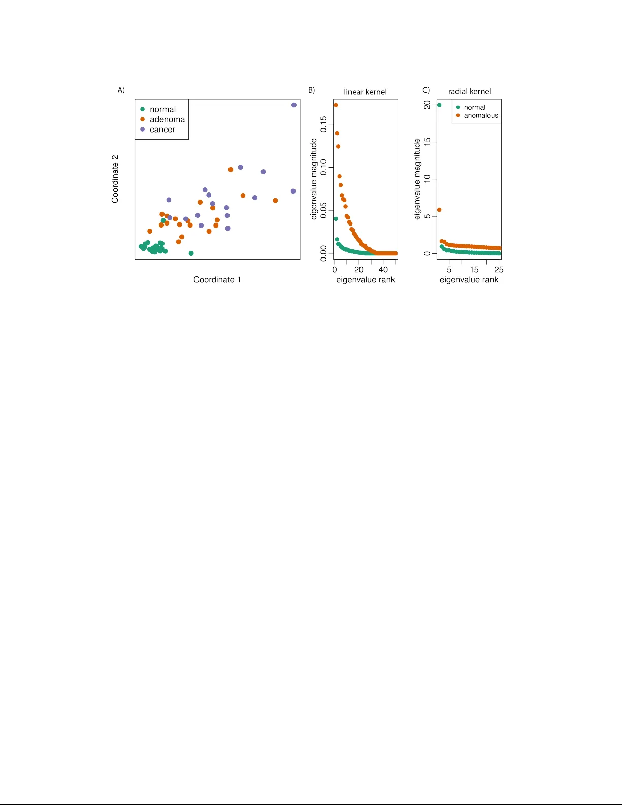
Anomaly Classification with the Anti-Pr ofile Support V ector Machine Wikum Dinalankara Center for Bioinformatics and Computational Biology Department of Computer Science Univ ersity of Maryland College P ark, MD 20742 wikum@cs.umd.edu H ´ ector Corrada Brav o Center for Bioinformatics and Computational Biology Department of Computer Science Univ ersity of Maryland College P ark, MD 20742 hcorrada@umiacs.umd.edu Abstract W e introduce the anti-profile Support V ector Machine (apSVM) as a nov el al- gorithm to address the anomaly classification problem, an extension of anomaly detection where the goal is to distinguish data samples from a number of anoma- lous and heterogeneous classes based on their pattern of deviation from a normal stable class. W e show that under heterogeneity assumptions defined here that the apSVM can be solved as the dual of a standard SVM with an indirect kernel that measures similarity of anomalous samples through similarity to the stable normal class. W e characterize this indirect kernel as the inner product in a Reproduc- ing Kernel Hilbert Space between representers that are projected to the subspace spanned by the representers of the normal samples. W e show by simulation and application to cancer genomics datasets that the anti-profile SVM produces clas- sifiers that are more accurate and stable than the standard SVM in the anomaly classification setting. 1 Introduction The task of anomaly , or outlier, detection [12, 8, 1] is to identify data samples that de viate signifi- cantly from a class for which training samples are av ailable. W e explore anomaly classification as an extension to this setting, where the goal is to distinguish data samples from a number of anomalous and heterogeneous classes based on their pattern of deviation from a normal stable class. Specifi- cally , presented with samples from a normal class, along with samples from 2 or more anomalous classes, we want to train a classifier to distinguish samples from the anomalous classes. Since the anomalous classes are heterogeneous using deviation from the normal class as the basis of classifi- cation instead of building a classifier for the anomalous classes that ignores samples from the normal class may lead to classifiers and results that are more stable and reproducible. The motiv ation for exploring this learning setting is from recent results in cancer genomics [3]. In particular , it was shown that hyper-v ariability in certain genomic measurements (DN A methylation and gene expression) in specific regions is a stable cancer mark across many tumor types. Further- more, this hyper-v ariability increases during stages of cancer progression. This led us to the question 1 Figure 1: (A) Principal component analysis of DN A methylation data [3]. V ariability in methylation measurements increases from normal to benign lesions (adenoma) to malignant lesions (cancer). The heterogeneity of the adenoma and cancer anomalous samples is the defining feature of the anomaly classification setting. (B) and (C) illustration of the heterogeneity assumption in Definition 1. For both a linear and radial basis function kernel, the magnitude of eigenv alues of the kernel matrix is larger for the anomalous classes. of how to distinguish samples from dif ferent stages in the presence of hyper-v ariability . In essence, how to distinguish samples from different anomalous classes (giv en by cancer progression stage) based on deviation from a well-defined normal class (measurements from non-cancerous samples). W e introduce the anti-profile Support V ector Machine (apSVM) as a novel algorithm suitable for the anomaly classification task. It is based on the idea of only using the stable normal class to define basis functions over which the classifier is defined. W e show that the dual of the apSVM optimization problem is the same as the dual of the standard SVM with a modified kernel function. W e then show that this modified kernel function has general properties that ensure better stability than the standard SVM in the anomaly classification task. The paper is organized as follows: we first present the anomaly classification setting in detail; we next describe the Anti-Profile Support V ector Machine (apSVM), and show that the dual of the opti- mization problem defined by it is equiv alent to the dual of the standard SVM with a specific kernel modification; we next show that this kernel modification leads directly to a theoretical statement of the stability of the apSVM compared to the standard SVM in the anomaly classification setting; we next show simulation results describing the performance and stability of the apSVM; and finally , we present results from cancer genomics showing the benefit of approaching classification problems in this area from the anomaly classification point of view . 2 The anomaly classification problem W e present the anomaly classification problem in the binary case, with two anomalous classes. Assume we are giv en training samples in R p from three classes: m datapoints from normal class Z , and n training datapoints as pairs h x 1 , y 1 i , . . . , h x n , y n i with labels y i ∈ {− 1 , 1 } indicating membership of x i in one of tw o anomalous classes A − and A + . Furthermore, we assume that the anomalous classes are heterogeneous with respect to normal class Z . Figure 1a illustrates this learning setting for DNA methylation data [3] (see 5 for details on this aspect of cancer epigenetics). It is a two-dimensional embedding (using PCA) of DNA methylation data for normal colon tissues along with benign growths (adenomas) and cancerous growths (tumor). V ariability in these specific measurements increases from normal to adenoma to tumor . W e would lik e to build stable and robust classifiers that distinguish benign growths from tumors. 2 Next we seek to formalize the heterogeneity assumption of the anomaly classification problem. In- tuitiv ely , the heterogeneity assumption we make is that given random samples of the same size from the normal class and from the anomalous classes, in expectation, the sample co variance of the anomalous samples is always larger than the cov ariance of the normal samples. W e state our assumption in the case of Reproducing Kernel Hilbert Spaces (RKHS) since we will use this ma- chinery throughout the paper [10, 14]. Recall that in a Bayesian interpretation of this setting, the kernel function associated with a RKHS serves as the co v ariance of a Gaussian point process. Definition 1 (Heterogeneity Assumption) . Let H be a Reproducing K ernel Hilbert Space with associated kernel function k . Let K m Z and K m A be the kernel matrices resulting from ev aluating the kernel function for a sample of size m of points in the normal and anomalous classes respecti vely . The heterogeneity assumption is that for every inte ger m , there exists  ∈ R , where 0 <  < 1 such that E det K m Z det K m A <  . Figures 1b and c show that the heterogeneity assumption is satisfied in the DNA methylation data for both linear and radial basis function kernels. Each figure sho ws the magnitude of the eigen values of the resulting kernel matrices. The magnitude of the eigen values in both cases is larger for the anomalous classes. The heterogeneity assumption gi v es us a hint to construct classifiers that deal with the heterogeneity of the anomalous classes. In Section 3.4 we sho w that heterogeneity has an impact on rob ustness and stability of classifiers built from training sets of the anomalous classes. Our goal is to use samples from the stable normal class to create classifiers that are robust. W e describe the anti-profile SVM as an extension to Support V ector Machines that accomplishes this goal. 3 The anti-profile SVM Support V ector Machines(SVMs) are one of the primary machine learning tools used for classi- fication. SVMs operate by learning the maximum-margin separator between two groups of data provided at training time. Any new observation provided to the SVM is classified by determining which side of the separator the new observ ation lies in. An important advantage of SVMs is that by applying the kernel trick, it is possible to find a hyperplane in a higher dimensional space where the two given classes are linearly separable, ev en when they are not linearly separable in their original feature spaces, and by virtue of the kernel trick this computation can be performed at no significant cost. While primarily designed for binary classification, SVMs have been extended for many other problems, such as multi-class classification and function estimation. 3.1 The SVM as weighthed voting of basis functions Here we revie w SVMs from a function approximation perspectiv e [14]: consider a set of n obser- vations, each observation being drawn from X × Y , where X ∈ R p , and Y ∈ {− 1 , 1 } . Here p is the number of features in each observation, or the dimensionality of the feature space. Thus each observation consists of a pair h x i , y i i , x i ∈ R p and y i ∈ {− 1 , 1 } , for i = 1 ..n ; here y i indicates which of the two classes the observation belongs to. If we introduce a new observation x 0 which needs to be classified, then the classification problem amounts to comparing x 0 to the e xisting set of points and combining the comparisons to make a decision. T o mak e the comparisons between observations, we make use of a similarity function. Let k ( x i , x j ) be a positive-definite similarity function which compares two points x i , x j ∈ R p . W eighing the similarity of the new observation to each existing observation, the dif ference of the sum of weighted similarities for the two groups will provide the necessary classification: g ( x ) = d + P n i =1 c i k ( x, x i ) . Here c i ≥ 0 ∀ i is the weight associated with each point, and d is a bias term. Classification is then based on the sign of the expansion: f ( x ) = sg n [ g ( x )] . Usually in SVMs function k is further assumed to hav e the reproducing property in a Reproducing Kernel Hilbert Space H associated with k : h f , k ( x, · ) i H = f ( x ) for all f ∈ H , and in particular h k ( x, · ) , k ( y , · ) i H = k ( x, y ) . In this case, the basis functions in the classifier correspond to repre- senters k ( x, · ) . In the standard SVM, the representers of all training points are potentially used as basis functions in the classifier , but effecti vely only a small number of representers are used as basis functions, namely the Support V ectors. Howe ver , for a giv en problem, we may choose a dif ferent 3 set of points for the deriv ation of the set of basis functions; the basis functions determine how the similarities are measured for a new point. 3.2 The Anti-Profile SVM optimization pr oblem The core idea in the anti-rofile SVM (apSVM) is to make use of this characterization of the Support V ector Machine as a linear expansion of basis functions defined by representers of training samples. In order to address the heterogeneity assumption underlying the anomaly classification problem we define basis functions only using samples from the stable normal class. Formally , we restrict the set of functions av ailable to define the subspace of H spanned by the representers of samples z 1 , . . . , z m from normal class Z : f ( x ) = d + P m i =1 c i k ( z i , x ) . T o estimate coefficients c i in the basis expansion we apply the usual regularized risk functional based on hinge loss R reg ( f ) = 1 n n X j =1 (1 − y i f ( x i )) + + λ 2 k h k 2 H , where ( · ) + = max(0 , · ) , f ( x ) is defined as f ( x ) = d + h ( x ) , and λ > 0 is a regularization parameter . By the reproducing kernel property , we have in this case that k h k 2 H = c 0 K n c where K n is the kernel matrix defined on the m normal samples. The minimizer of the empirical risk functional is giv en by the solution of a quadratic optimization problem, similar to the standard SVM, but with two kernel matrices used: K n , defined in the pre- vious paragraph, and K s , which contains the e valuation of kernel function k between anomalous samples x 1 , . . . , x n and normal samples z 1 , . . . , z m : min d,c,ξ e T ξ + nλ 2 c T K n c (1) s.t. Y ( K s c + de ) + ξ ≥ e, ξ ≥ 0 Here we use slack variables ξ = ( ξ 1 , ξ 2 , ..., ξ n ) 0 , denote the unit vector of size n as e , and define matrix Y as the diagonal matrix such that Y ii = y i . 3.3 Solving the apSVM optimization problem The Lagrangian of problem 1 is giv en by L ( c, d, ξ , α, β ) = e T ξ + nλ 2 c T K n c − α T [ Y ( K s c + de ) + ξ − e ] − β T ξ where α n × 1 = ( α 1 , ..., α n ) T and β n × 1 = ( β 1 , ..., β s ) T are the Lagrangian multipliers. Minimizing with respect to z , c and d , we find that the W olfe dual of problem 1 is max α e T α − 1 2 nλ α T Y ˜ K Y α (2) s.t. 0 ≤ α ≤ e, e T Y α = 0 where ˜ K = K s K − 1 n K T s . Here we assume K − 1 n represents a pseudo-in verse in the case where K n is not positiv e definite. For a standard SVM, the objecti v e of the W olfe dual is e T α − 1 2 nλ α T Y K Y α , with K the kernel ma- trix the training datapoints. Thus the dual problem of the apSVM has the same form as the standard SVM dual problem with the exception that k ernel matrix K is replaced by induced kernel matrix ˜ K in the apSVM. Kernel matrix ˜ K essentially represents an indirect kernel between anomalous sam- ples induced by the set of basis functions determined by the samples from the normal class. Since the essential form of the SVM solution is unchanged by the modification, this provides the addi- tional advantage that the modified SVM can be solved by the same tools that solve a regular SVM, 4 but with a different kernel matrix provided. For our particular problem domain, we use the indirect kernel to represent deviation from the profile of normal samples, and thus refer to this classifier as the anti-profile SVM. 3.4 Characterizing the indirect k ernel W e sa w abov e that the apSVM can be solved as a standard SVM with induced k ernel ˜ K = K s K − 1 n K T s . In this section we characterize this indirect kernel, and state a general result that eluci- dates how the apSVM can produce classifiers that are more robust and reproducible that a standard SVM in this setting. Proposition 1. Let P Z be the linear operator that pr ojects r epr esenters k ( x, . ) ∈ H to the space spanned by the r epr esenters of the m normal samples of the anomaly classification pr oblem. Induced kernel ˜ k satisfies ˜ k ( x, y ) = k ( P Z k ( x, . ) , P Z k ( y , . )) . Pr oof. Projection P Z k ( x, . ) is defined as P Z k ( x, . ) = P m i =1 ˆ β i k ( z i , . ) where ˆ β = arg min β 1 2 k k ( x, . ) − X i β k ( z i , . ) k 2 H = arg min β 1 2 h k ( x, . ) − X i β k ( z , . ) , k ( x, . ) − X i β k ( z i , . ) i H = arg min β 1 2   X i,j h k ( z i , . ) , k ( z j , . ) i H − X i h k ( x, . ) , k ( z i , . ) i H   = arg min β 1 2  β T K n β − k T z x β  , (3) where k z x is the vector with element i equal to k ( z i , x ) . From (3) we get ˆ β = K − 1 n k z x . Therefore h P Z k ( x, . ) , P Z k ( y , . ) i H = k T z x K − 1 n k z y = ˜ k ( x, y ) . This proposition states that the indirect kernel is the inner product in Reproducing K ernel Hilbert Space H between the representers of anomalous samples projected to the space spanned by the representers of normal samples. By the heterogeneity assumption of Definition 1, the space spanned by any subset of anomalous samples will be smaller after the projection. In particular, the smallest sphere enclosing the projected representers will be smaller , and from results such as the V apnik- Chapelle support vector span rule [13], classifiers built from this projection will be more rob ust and stable. 4 Simulation Study W e first present simulation results that sho w that the apSVM obtains better accuracy in the anomaly classification setting while providing stable and robust classifiers. W e generated samples from three normal distributions as follows: if A + and A − are the anomalous classes that we need to distinguish, and Z is the normal class, then for a giv en feature we dra w datapoints from distrib utions Z = N (0 , σ 2 N ) , A − = N (0 , σ 2 A − ) and A + = N (0 , σ 2 A + ) . T o simulate our problem setting, we set σ 2 Z < σ 2 A − < σ 2 A + . Results hav e been obtained from tests written on R (version 2.14) with R packages kernlab (v ersion 0.9-14) [7] and svmpath (version 0.952). The svmpath tool provides a fitting for the entire path of the SVM solution to a model at little additional computational cost [4]. Using the resulting fit, the SVM classifications for any gi ven cost parameter can be obtained. For our experiments, the testing set accuracy was computed for each value of cost along the regularization path, and the best accuracy possible was obtained; ties were broken by considering the option with the least number of support vectors used. Note that a small ridge parameter (1e-10) was used in the svmpath method to av oid singularities in computations. 5 Figure 2: (A) Accuracy results in simulated anomaly classification data. The anti-profile SVM achiev es better accuracy than the standard SVM. (B) Stability results in simulated data. The anti- profile SVM uses a smaller proportion of training points as support vectors. SVMs that use fewer support vectors are more rob ust and stable. Each training set contained 20 samples from each of A − and A + classes, while each testing set contained 5 samples from each class; 20 samples from class Z were used for the anti-profile SVM. For a giv en number of features, each test was run 10 times and the mean accuracy computed. T o estimate the hyperparameter for the radial basis kernel, the inv erse of the mean distance between 5 normal and 5 anomalous samples (chosen randomly) was used. Figure 2a sho ws the accurac y of a standard SVM and the apSVM using an RBF kernel for simulated data with σ Z = 1 , σ A − = 2 , σ A + = 4 . W ith a radial basis kernel, the anti-profile SVM was able to achiev e better classification than the regular SVM. W e characterize the stability of a classifier using the proportion of training samples that are selected as support vectors. Classifiers that use a small proportion of points as support vectors are more robust and stable to stochasticity in the sampling process. The more support vectors used by an SVM, the more likely it is that the classification boundary will change with any changes in the training data. Hence a boundary that is defined by only a few support v ectors will result in a more robust, reliable SVM. Figure 2b shows that in the simulation study the apSVM used fewer support vectors than the standard SVM while obtaining better accuracy . 5 A pplication to cancer genomics The motiv ation for this work is from recent studies of epigenetic mechanisms of cancer . Epigenet- ics is the study of mechanisms by which the expression level of a gene (i.e. the degree to which a gene can ex ert it’ s influence) can be modified without any change in the underlying DN A sequence. Recent results sho w that certain changes in DN A meth ylation are closely associated with the occur - rence of multiple cancer types [3]. In particular , the existence of highly-variable DN A-methylated regions in cancer as compared to normals(i.e. healthy tissue) has been shown. Furthermore, these highly-variable regions are associated with tissue differentiation, and are present across multiple cancer types. Another important observation made there is that adenomas, which are benign tumors, show intermediate levels of hyper-v ariability in the same DN A-methylated regions as compared to cancer and normals. This presents an interesting machine learning problem: distinguishing between cancer and adenoma based on the hyper-v ariability of their methylation lev els with respect to normal samples? A suc- cessful tool that can classify between the two groups can hav e far -reaching benefits in the area of personalized medicine and diagnostics. Since the tw o classes are essentially dif ferentiated by the de- gree of v ariability the y exhibit with respect to normals, for our purpose we can abstract the problem to the setting we present here as anomaly classification. 6 Figure 3: Classification results for DN A methylation in cancer [3]. While both a standard SVM and the anti-profile SVM achiev e similar accuracy using an RBF kernel (A), the anti-profile SVM uses much fewer support v ectors. 5.1 Methylation data r esults W e study the performance of the apSVM in a dataset of DN A methylation measurements obtained for colon tissue from 25 healthy samples, 19 adenoma samples, and 16 cancer samples, for 384 spe- cific positions in the human genome [3]. As mentioned previously , the cancer samples exhibit higher variance than healthy samples, with adenoma samples showing an intermediate lev el of variability (Figure 1). W e used the same classification methods mentioned in the previous section, but with multiple runs, for each run randomly choosing 80% of tumor samples for training and the remaining for testing. Figure 3 sho ws the results obtained using a radial basis kernel. While the indirect k ernel performs either at the same le v el or marginally better than the regular kernel, then anti-profile SVM uses much less support vectors than the standard SVM, thus providing a much more robust classifier . 5.2 Expression data r esults W e further applied our method to gene expression data obtained with a clinical experiment on adrenocortical cancer [2]. The data contains expression lev els for 54675 probesets, for 10 healthy samples, 22 adenoma samples, and 32 cancer samples. The data sho ws the same pattern with re gard to hyper-v ariability as the methylation data. Using the same methods as before, the results obtained using a linear kernel are sho wn in Figure 4. For feature selection, the features were ranked according to log v ar( C arcinoma ) v ar( Adenoma ) and for a gi ven number n as the number of features to be used, n features with the highest v ariance ratio were selected. While both the standard SVM and the apSVM provided almost perfect classification, there is a significant difference in the number of support vectors used, with the indirect kernel requiring much fewer support vectors and hence providing a more stable classifier . 6 Discussion W e have introduced the anti-profile Support V ector Machine as a novel algorithm to address the anomaly classification problem. W e hav e shown that under the assumption that the classes we are trying to distinguish with a classifier are heterogeneous with respect to a third stable class, we can define a Support V ector Machine based on an indirect kernel using the stable class. W e hav e shown that the dual of the apSVM optimization problem is equiv alent to that of the standard SVM with the addition of an indirect kernel that measures similarity of anomalous samples through similarity to the stable normal class. Furthermore, we hav e characterized this indirect kernel as the inner product in a Reproducing K ernel Hilbert Space between representers that are projected to the subspace spanned by the representers of the normal samples. This led to the result that the apSVM will learn classifiers that are more robust and stable than a standard SVM in this learning setting. W e ha v e sho wn by simulation and application to cancer genomics datasets that the anti-profile SVM does in fact produce classifiers that are more accurate and stable than the standard SVM in this setting. 7 Figure 4: Classification results for gene expression in cancer [2]. Similar to Figure 3, the accuracy of both the standard and anti-profile SVM is similar (in this case almost perfect testset accuracy is achiev ed by both classifiers). Howe v er , the anti-profile SVM again uses fewer support vectors, leading to classifiers that are more robust and stable. While the motiv ation and examples provided here are based on cancer genomics we expect that the anomaly classification setting is applicable to other areas. In particular, we hav e started looking at the area of statistical debugging as a suitable application [16]. The characterization of the indirect kernel through projection to the normal subspace also suggests other possible classifiers suitable to this task. For instance, by defining a margin based on the projection distance directly . Furthermore, connections to kernel methods for quantile estimation [11] will be interesting to explore. Another direction of interesting research would be to further solidify the stability characterization we provide in Section 3.4. For instance, by e xploring the relationship to other lea v e-one-out bounds [9, 6, 15, 5], and the span rule for kernel quantile estimation [10]. References [1] V arun Chandola, Arindam Banerjee, and V ipin Kumar . Anomaly detection: A survey . ACM Comput. Surv . , 41(3):15:1–15:58, July 2009. ISSN 0360-0300. doi: 10.1145/1541880. 1541882. URL http://doi.acm.org/10.1145/1541880.1541882 . [2] Thomas J Giordano, Rork Kuick, T obias Else, Paul G Gauger , Michelle V inco, Juliane Bauers- feld, Donita Sanders, Dafydd G Thomas, Gerard Doherty , and Gary Hammer . Molecular clas- sification and prognostication of adrenocortical tumors by transcriptome profiling. Clinical cancer r esear ch : an official journal of the American Association for Cancer Resear ch , 15(2): 668–676, January 2009. [3] Kasper Daniel Hansen, W inston T imp, H ´ ector Corrada Brav o, Sarven Sabunciyan, Benjamin Langmead, Oliver G McDonald, Bo W en, Hao W u, Y un Liu, Dinh Diep, Eirikur Briem, Kun Zhang, Rafael A Irizarry , and Andrew P Feinberg. Increased methylation variation in epige- netic domains across cancer types. Nature Genetics , 43(8):768–775, August 2011. [4] T rev or Hastie, Saharon Rosset, Robert T ibshirani, and Ji Zhu. The Entire Regularization Path for the Support V ector Machine. The Journal of Machine Learning Researc h , 5:1391–1415, December 2004. [5] T . Jaakkola and D. Haussler . Probabilistic kernel regression models. Proceedings of the 1999 Confer ence on AI and Statistics , 1999. [6] T . Joachims. Estimating the generalization performance of a SVM efficiently. Pr oceedings of the International Confer ence on Machine Learning , 2000. [7] Alexandros Karatzoglou, Alex Smola, Kurt Hornik, and Achim Zeileis. kernlab – an S4 package for kernel methods in R. Journal of Statistical Softwar e , 11(9):1–20, 2004. URL http://www.jstatsoft.org/v11/i09/ . 8 [8] Larry M. Manevitz and Malik Y ousef. One-class svms for document classification. J . Mach. Learn. Res. , 2:139–154, March 2002. ISSN 1532-4435. URL http://dl.acm.org/ citation.cfm?id=944790.944808 . [9] M. Opper and O. Winther . Gaussian Processes for Classification: Mean-Field Algorithms. Neural Computation , 12:2655–2684, 2000. [10] B. Scholkopf and A.J. Smola. Learning with Kernels . MIT Press Cambridge, Mass, 2002. [11] B Sch ¨ olkopf, J C Platt, J Shawe-T aylor, A J Smola, and R C Williamson. Estimating the support of a high-dimensional distrib ution. Neural computation , 13(7):1443–1471, July 2001. [12] Ingo Steinwart, Don Hush, and Clint Scovel. A classification framework for anomaly detection. J. Mach. Learn. Res. , 6:211–232, December 2005. ISSN 1532-4435. URL http://dl. acm.org/citation.cfm?id=1046920.1058109 . [13] V . V apnik and O. Chapelle. Bounds on Error Expectation for Support V ector Machines. Neural Computation , 12:2013–2036, 2000. [14] G. W ahba. Support vector machines, reproducing kernel Hilbert spaces, and randomized GA CV. Advances in kernel methods: support vector learning , pages 69–88, 1999. [15] G. W ahba, Y . Lin, Y . Lee, and H. Zhang. On the relation between the GA CV and Joachims’ ξ α method for tuning support vector machines, with extensions to the nonstandard case. T echnical report, T echnical Report 1039, Statistics Department University of W isconsin, Madison WI, 2001, 2001. [16] AX Zheng, MI Jordan, and B Liblit. Statistical debugging of sampled programs. Advances in Neural Information Pr ocessing Systems , 16, 2003. 9