Perceptive Statistical Variability Indicators

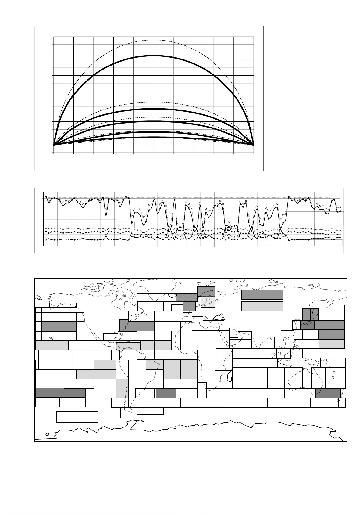
1 Perceptive Statistical Variability Indicators Kalman Ziha University of Zagreb, Faculty of Mechanical Engine ering and Naval Architecture, De partment of Naval Architectu re and Ocean Engineering, Ivana Lucica 5, 10000 Zagreb, Croatia E-mail: kziha@fsb.hr Tel: +385 1 6168132 Fax: +385 1 61656940 Abstract: The concepts of variability and uncertaint y, both epistemic and alleatory, came from experience and coexist with different connotations. Therefore this article attempts to express their relation by analytic means firstly setting si ghts on their differences and then on their common characteristics. Inspired with the alternative expression of uncertain ty defined as the average number of equally probable events based on entropy concept in probability theo ry, the article introduced two related perceptiv e statistical measures which indicate the same vari ability and invariability as the basic probability distribution. First is the e quivalent number of a hypothetical distribution with one sure and all the other impossible outcomes which indicates variability. Sec ond is the appropriate e quivalent num ber of a hypothetically uniform distribution w ith all equal probabilities which i ndicates invariability. The article interprets the common properties of variab ility and uncertainty on theo retical distributions and on ocean- wide wind wave directional properties co mpiled in the Glob al Wave Statistics. Key words: variability; uncertainty; predic tabil ity, equivalent numbers, average num ber 2 1 Introduction The variability assessment of N discrete numbers y i , 1 , 2, ..., iN = , is a problem of lasting inte rest in statistics and elsewhere (e.g. Cramer, 1945, Ke nney and Keeping, 1951, Anderson and Bancroft, 1952, Hogg and Craig, 1965). A set of N normalized num bers i p , 1 , 2, ..., iN = can represent a discrete distribution of probabilities P (1) in the range ( p Min – p Max ) as shown: () 12 ,, , NN p pp =⋅ ⋅ ⋅ P ( 1 ) The disjoined random events j E with probabilities of events ) ( i i E p p = , 1, 2 , , iN =⋅ ⋅ ⋅ configure a system S N that can be written down after Khinchin (1957) in a form of an N -element finite schem e: () ( ) () () 12 11 2 2 jN N jj N N EE E E pp E p p E p p E p p E ⋅⋅⋅ ⋅⋅⋅ ⎞ ⎛ = ⎟ ⎜ ⎜⎟ = = ⋅⋅⋅ = ⋅⋅⋅ = ⎝ ⎠ S ( 2 ) The probability of a distribution of N probabilities P N (1) or of a system of N events S N (2) is then in general 1 () ( ) 1 N NN i i po r p p = =≤ ∑ PS . For a complete distribution is ( ) ( ) 1 NN po r p = PS . 2 Variability of probabilities of probability dist ributions For generally partial distributions P N (1) the mean value of N probabilities is: () ( 1 / ) () NN pp N p == ⋅ PP ( 3 ) The average variance V ( P N ) of N probabilities p of a distribution P N (1) reads: 22 2 2 11 () () ( 1 / ) ( ) ( 1 / ) NN NN i i ii VN p p N p p σ == == ⋅ − = ⋅ − ∑∑ PP ( 4 ) The article considers next a propos al for a reference value of vari ance (4) in order to describe a probability distribution when one probability () j N pp → P is dominant and all the others 0 → ≠ j i p for 1, 2 , 1 iN =⋅ ⋅ ⋅ − are vanishing. The reference value o f varian ce can be then calculated by definition as: 2 Ref () 0 () l i m () () ( 1 ) / j ij NN N pp p VV p N N ≠ → → == ⋅ − P PP P ( 5 ) Appendix A presents the proof that the reference va riance (5) is the maxim ally attainable value. The coefficient of variation of N probabilities of a dist ribution of probabilities P N (1) it reads: () () / NN CV p σ = PP ( 6 ) 3 The coefficient of variation of N probabilities (6) has c ontinuity in its arguments, m onotonic increase with the number of outcomes up to limiting value Ref () 1 CV N = − P and a composition rule based on additivity rule of variances. Im possible occurrenc es with ze ro probability do not influence affect variability (6) but the in co mpleteness of distributions p N ( P )<1 affects variability (4). The coef ficient of variation of N probabilities (6) of a di stribution of probabilities P N (1) can be appropria tely presented also by its relative value () () / 1 NN cv CV N =− PP . For a range of discrete random variables n= 1, 2, 5, 10 and 50 and for a range of probabilities p from 0 to 1, the variability of binomial distributions is presented by the coefficient of variation (6), (Fig. 1). 3 Uncertainty of systems of events The concept of entropy has been introduced earlier in inform ati on theory for assessment of the amount of information pertinent to system of events S N (2) (Hartley, 1928, Shannon and Wiever, 1948). The entropy has been lately applied in probability theory to define the uncertainties of systems of events S N (2) (Khinchin, 1957, Renyi, 1970, Aczel and Daroczy , 1975). Entropy defines the uncertainty of th e observable properties that turns into inform ation when observations becom e available. The entropy of a single event is defined as the l ogarithm of the equivalent number of events 1 / ( ) i p E with equal probability [ ] 2 ()l o g 1 / () ii E pE μ = and can be interpreted accordi ng to Wiener (1948) either as a measure of the information yielded by the even t E i or how unexpected the event was. The uncertainty of a complete system S N (2) of N events can be expressed as the weighted sum of unexpectednesses of all events by the Sh annon’s entropy (Shannon and Weaver, 1949): 11 () l o g NN Nj j j j jj Hp p p μ == =⋅ = − ∑∑ S ( 7 ) According to Cover and Thomas (2006) the Shannon's information entropy H has a number of natural properties for notions of uncertainty : continuity in its arguments, m onotonic increase with the number of equi-probable outcomes and a composition rule. Th e uncertainty of an incomplete system of N events S N (2) can be defined as the limiting case of the Renyi ’s entropy (1970) of order 1 using (3) and (7) as: 1 1 1 () l o g () N R Nj j j Hp p p = =− ∑ S S ( 8 ) 4 Shannon's axiomatic derivation of entropy explains (1949) why it is the intuitive measure of uncertainty. In addition, the uniqueness theorem by Khinchin (1957) proves that the entropy is the only function that measures the probabilistic uncertainty of systems of events in agreement with the experience of uncertainty. The theorem of mixture of distri butions (Khinchin, 1957; Renyi, 1970) provides the conditional (average) entropy of system S with respect t subsystems of events. The uncertainty of systems of events S (2) for binomial distributions for a range of probabilities p from 0 to 1 and for numbers of variables n= 1, 2, 5, 10 , and 50 is presented by the entropy (7) (Fig. 1). 5 Average numbers of events and equivalent numbers of outcomes Aczel and Daroczy mentioned earlier (1975) the av erage number of equally probable events th at follows from the condition of maximal uncertainty 2 () l o g () NN HF = SS as an uncertainty indicator: () () 2 N H N F = S S ( 9 ) The average number of events () N F S (9) in the range N F N ≤ ≤ ) ( 1 S is not any more dependent on the base of applied logarithm. It defines a hypot hetically uniform probability distribution of F N equal probabilities amounting to 1/ F N with same uncertainty as the entropy () N H S of the system S (Fig. 2). Relative measures such as ( ) ( ) / l og NN hH N = SS (7, 8) or (9) ( ) ( ) / NN f FN = SS can be appropriate. The concept of average numbers of events based on entropy (9) has inspired the investigation of equivalent numbers of outcom es based on statistical variability of probability distributions (3-6). The article firstly concentra tes on variability of probability distribu tions. Therefore it defines the equivalent number G N ( P ) of a hypothetical probability di stribution with one sure and remaining G N ( P )-1 impossible outcomes which provides the sam e variability as the basic distribution P of N probabilities (Fig. 2). The equivalent number G N ( P ) follows directly from the condition that the coefficient of variation CV N ( P ) (6) is equal to its maxim al value () 1 N G − P , as it is shown below: 2 () () 1 NN GC V =+ PP ( 1 0 ) In the context of this research the square 2 () N CV P of the coefficient of variation (6) of any probability distribution P (1) or a system of events S (2) in (1 0) represents the num ber of im possible outcomes or 5 events in addition to a single sure outcom e or certain event that prov ide the same varia bility or certainty as the original probability distribut ion of N outcomes or the system of N events. The article next focuses on invariability of pr obability distributions. The equivalent number D N ( P ) of equal probabilities in amount of 1/ D N ( P ) of a hypothetically complete pr obability distribution expresses the invariability when the variance (4 ) of a distribution P (1 ) of N probabilities is equal to zero [] 22 1 1/ ( ) 1/ ( ) 0 N Ni N i Dp D = ⋅− = ∑ PP (Fig. 2), as it is shown below: () 22 2 1 () 1 / / () () 1 N Ni N N i Dp N p C V = ⎡⎤ == ⋅+ ⎣⎦ ∑ PP P ( 1 1 ) In the context of this res earch the sum of squares of probabilities 2 1 N i i p = ∑ in (4) of any probability distribution P (1) or a system of events S (2) in (11) represents the mean probability of a hypothetically uniform probability distribution or a system of events of D N ( P ) equally probable outcomes or events. The following relation links the two equivalent num bers for generally incomplete distributions with known probability p N ( P ) of N possible outcomes: 2 () () / () NN N DG N p ⋅= PP P ( 1 2 ) The relation (12) in logarithmic f orm expresses uncertainties as shown: log ( ) log ( ) log 2 ( ) NN N D G N logp += − PP P ( 1 3 ) The terms (9), (10) and (11) im ply the generalization of number of events other than integers. The increasing number of impossible outcom es in the range 0( ) 1 1 N GN ≤ −≤ − P (10) with respect to one sure outcome based on CV N ( P ) (6) indicates increasing v ariability and rise of predictability. On the other hand, the increasing value of equivalent number of equally pr obable outcomes (11) in the range 1( ) N DN ≤≤ P (11) indicates lessening variability a nd a drop of predictability (Table 1). Simultaneously, the average num ber of equally probable events (9) in the range 1 ( ) N FN ≤≤ S based on entropy (7, 8) represents rise in uncertainty and as such indicates drop of predictability (Table 1). Thus, the equivalent numbers of outcomes ( ) N D P (11) and the average numbers of events ( ) N F P (9) go well together in expressing the invariability-uncer tainty-unpredictability (Table 1). 6 The increasing equivalent probability in the range ( ) 1/ 1/ 1 N ND ≤ ≤ P based on statistical invariability (11) expressing the g rowth of i nvariability and the average p robability 1 / 1 / ( ) 1 N NF ≤≤ S based on probabilistic entropy (7, 8) represen ting the dr op of uncertainty, indicate rise of predictability. Hence, he equivalent numbers of events ( ) N G P (9) go well together with equivalent ( ) 1/ N D P and average 1 / ( ) N F S probabilities in expressing the variabil ity-cer tainty-predictability (Table 1). The difference between analytical defi nitions of variability (10) and unc ertainty (9) is in perception of impossible or certain events. The unc ertainty (9) vani shes whenever there is at leas t one certain event regardless of the number of impossible events. Howeve r, when any one event is su re, the variability perception (10) depends on the number of remaining im possible events since the m ean value of the distribution of probabil ities changes with overa ll num ber of outcomes. Statistical properties (3 -6) of distributions of probabilities P N (1), the entropy (7, 8) of systems of events S N (2) or the average and equivalent numbers (9, 10, 11) do not depend on sequences of probabilities. Variability and uncer tainty are commonly considered as objectiv e properties since they depend on nothing else but on the probability distributi ons. Therefore th e intrinsic predictability ba sed on statistical variability can be considered as an objective p roperty too. However, probabilistic forecasts can be performed with conditional distributions empl oying posterior distributi ons. The common posterior verification method for proba bilistic forecasts is the Brier score (1950) proposed as the averag e deviation between predicted proba bilities for a set of events and their outcomes. R elative measures of predic tability can be also important given that a Bayesian viewpoint of prediction is a useful one. In that context the relative entropy is useful and wo rth considering, e.g. Kleeman (2002), Roulston&Smith (2002) and Bröcker (2009). This of course involves both prior and posteri or distributions. 6 Variability and uncertaint y of wind wave climate Visual observations of wind speeds (Beaufort Scale) and directions and wave heights have been reported since 1854; observations of commercial ship s have been archived since 1861; wave height, period and directions have been reported from ship s in norm al service all over the world since 1949. The observations are systematically collected followi ng the non-instrum ental me thodology prescribed since 7 1961 by the resolution of the World Me teorological Organization (W MO) in order to assure that the data are globally homogeneous in quality and coverin g most sea areas of practical interes t for shipping, navigation, towing and offshore activities. The comp ilation of these observations for each of the N A =104 Marsden’s squares (Fig. 4) is th e Global W ave St atistics (GWS) prepared by Hogben, Dacunha & Ollive r (1986) that uses the past expe riences to eliminate biases. The study in the sequel investigates the variability of wave dir ections based on annual wind wave climate observation reported in the G WS (1986) by probability distributions in 104 ocean areas A (Fig. 4 and 6) as 8 ( ) (d , d , d , d , d , d , d , d ) NN E E S E SS W WN W A = P of N =8 principal wave directions. For wind wave climate directional obse rvations circular statistics is appropriate, e.g. Fisher (1993). However, the variability of probabil ities of wind wave directions is not necessarily of ci rcular character and linear descriptiv e statistics can be applied. The article firstly graphically presents the eq uivalent numbers of directions D 8 [ P (A) ] (11), the average number of events F 8 [ P (A) ] (9) with respect to th e nominal num ber of directions N =8 for all ocean areas (Fig. 3). The two numb ers indicate sam e ordering base d on variability and uncertainty considerations. The same graph also presents the rela tive uncertainty h 8 [ P (A) ] (8),and the statistical va riability of probabilities of wave directions cv 8 [ P (A) ] (6) which indicate opposite ordering (Fig. 3). The article next presents the chart of the relativ e probabilistic statistical va riability cv 8 [ P (A) ] (6) (F ig. 4) and the chart of equivalent numbers of events D 8 [ P (A) ] (11) (Fig. 5) of wind wave directions. There follows few comments. The wave directions are highly predictabl e in some areas in the eastern Pacific Ocean such as A64 given by distribution P 8 ( A64)=(0.0042 0.0098 0.1151 0.6081 0.2110 0.0234 0.0049 0.0033) where cv 8 (A64) ∼ 60% ] (Fig. 4). The three directions (east, south-east and south) prevail with about 90% (Fig. 6). The appropria te equivalent number of wave directions D 8 (A64)=2.3 (Table 2 and Fig. 5) indicates inva ria bility of directions equivalent to probabil ity distributions with numbers of equally probab le outcomes between two P 8 (A64)=(1/2 1/2) and three P 8 (A64)=(1/3 1/3 1/3), closer to two than to three. Th e average number of wave directions F 8 (A64)=3 (Table 2) indicates uncertainty appropriate to pr obability distributions with th ree equally probable outcomes. 8 The appropriate equivalent number of wave directions G 8 (A64)=3.6 (Table 2 a nd Fig. 6) indicates variability equivalent to a probability distributions with number of outcomes from which one is sure and two P 8 (A64)=(1 0 0) or three P 8 (A64)=(1 0 0 0) are im possible. Simila r is the situation in som e areas of western Atlantic Ocean such as A66, A67 and A68. In some ocean areas the wave directions are unpred ictable sin ce the directions are almost uniform ly distributed. For example in South Pa cific area A86 the probability dis t ribution of wave directions is P 8 (A86)=(0.1192 0.0941 0.1157 0.1125 0.1299 0.1370 0. 1489 0.1152) and the relative coefficient of variation is only cv 8 (A86)=4.75%. There, the equivalent number of wave directions D 8 (A86)=8.3 and the average number of wave directions F 8 (A86)=8.2 (Table 2 and Fig. 7) even exceeds the nom inal value of N =8 due to incompleteness of observations. This indica tes tha t the equivalent probability distribution is P 8 (A86)=(1/8 1/8 1/8 1/8 1/8 1/8 1/8 1/8). The appropriate equivalent number of wave directions G 8 (A86)=1.01 (Table 2 and Fig. 7) indicates almost m aximal variability, that is al most full certain ty, when one outcome is sure and another is close to be impossible G 8 (A86)=(1 0). Similar is th e situation in Nort h Atlantic area A1 where cv 8 (A1)=4.75%. 7 Conclusions Variability and uncertainty are recognizable as two opposite prope rties which naturally m otivate conscious observers of random phenomena for predictions . Therefore the article a dvocated two particular functionals using statistical variability defined on proba bility sets to b ring these two properties clo ser to common experience of randomness. The two types of equivalent num bers of outcomes or events were introduced with the aim to represent com mon indicat ors of invariability and cer tainty as well as variability and uncertainty, othe r than just statistical variance and probabilistic entropy. The properties of proposed indicators were premeditated to match hum a n comprehension of rando m phenom ena closely to everyone’s gambling perception of hazardous gam es. For example, it is intuitively p erceptive that the flipping of a balanced coin is as predictable as 2 events with probabi lities 1/2 and tossing of an unbiased dice as 6 events with probabilities 1 /6. The equi valent and average numbers im ply the analytical generalization of numbers of outcomes of probability di stributions or of numbers of events of systems of events for perceptive pr esentation o variability and uncertainty othe r than only integers. 9 References Aczel, J. and Daroczy, Z. 1975: On Measures of Info rmation and Their Characterization, Acad. Press, NY. Anderson, R.L. and Bancroft, T.A. 1952: Sta tistical Theory in Research, McGraw-Hill, NY. Brier, G. W. 1950: Verification of forecasts expressed in term s of probability, Monthly Weather Review, 75, 1-3. Broecker, J. 2009:. Reliability, suffciency and the decompos ition of proper scores. Q. J. R. Meteorol. Soc., 135. Cover, A. and J. A. Thomas, J.A. 2006: Elem ents of In formation Theory. Wiley-Interscience, Hoboken, 2 edition. Cramer, H. 1945: Mathematical Methods of Statistics, Princeton University Press. Fisher, NI. 1993: Statistical Analysis of Circular Data, Cambridge University Press. Hartley, R. V. 1928: Transmission of Information, Bell Systems Tech. J, 7 . Hogben, N., Dacunha N. M.C., Olliver G. F. 1986: Global Wave Statistics, British Maritim e Technology Feltham. Hogg R.V., Craig, A.T. 1965: Introduction to Mathe m atical Statistics, The MacMillan Company, NY. Kenney, J.F., Keeping, E.S. 1951: The Mathem ati cs of Statistics I&II, D. Van Nostrand Inc., London. Khinchin, A. I. 1957: Mathematical Foundations of Information Theory, Dover Publications, NY. Kleeman, R. 2002: Measuring dynamical prediction utility using relative entropy. J. Atmos. Sci., 59(13): 2057- 2072. Renyi, A. 1970: (tu fali space) Probab ility Theory, North-Holland, Amsterdam. Roulston, M.S. and Smith, L.A. 2002: Evaluating probab ilistic forecasts using information theory. Mon. Weather Rev., 130(6):1653-166 0, 2002. Shannon, C. E. and Weaver, W. 1949: The Mathematical Theory of Communication, Urbana Univ., Illinois. Wiener, N. 1948: Cybernetics or Control and Communication, Bell System Tech. J, 27 . Appendix A Let’s consider a com plete probability distribution of N probabilities 1 1 N i i p = = ∑ . From the Jensen inequality directly f ollows the lower lim it of the sum of squares of a probability distribution 2 1 1 N i i p N = ≤ ∑ . According to common reasoning for any 1 i p < is 2 ii p p < , and therefore the upper limit is 2 1 1 N i i p = < ∑ . Since only the unity has the property 2 11 = , the sum of squares attains its maximal value in am ount of 2 1 1 N i i p = = ∑ only if any of the probabil ities is equal to unity 1 i p = and all the other ( N -1) probabilities are zero 0 ji p ≠ = . 10 Table 1. Comparative properties of (in)variability a nd (un)certainty related to predictability Variability (Fig. 1) Coefficient of variation of probab ilities (6) 22 1 () / () 1 N NN i i CV N p p = ⎡⎤ =⋅ − ⎣⎦ ∑ PP Min: 0 – Invariable (All N outcomes equally probable) Max; 1 N − – Maximal variability (One sure outcome all N-1 others impossible) Unit: 1– (One sure outcome, one impossible N=2) Uncertainty (Fig. 1) The entropy of system of events (8) [] 1 () 1 / () l o g N Ni i i Hp p p = =− ∑ SS Min: 0 – Certain (One certain event, N-1 others impossible) Max; log N - Full uncertainty (All N events equally probable) Unit: 1 bit (Two equally probable events Invariability (Fig. 2) Equivalent number of outcom es (11) 22 1 () 1 / / () () N Ni N N i Dp N p G = ⎡⎤ == ⋅ ⎣⎦ ∑ PP P Range: 1 ( ) N DN ≤≤ P where 2 () () 1 NN GC V =+ PP Min: 1: Fully predictable/Certain One sure outcome, another impossible(N=2) CV=1 One sure outcome, N-1 impossible 1 CV N = − Max: N – Unpredictable/Uncertain CV =0 (All N outcomes are equally probable) Ref: 2: (Two equally probable events N=2) Certainty (Fig. 2) Average number of events (9) 1 lo g () () 2 2 N ii iN pp H N F = − ∑ == S S Range: 1( ) N FN ≤ ≤ S Min: 1: Certain/ Fully predictable One certain event, one impossible(N=2) H= 0 One certain event, N-1 impossible H= 0 Max: N –Uncertain/Unpredictable H =log N (All N events are equally probable) Ref: 2: (Two equally probable events N=2) Table 2 . Variability and uncertainty of wave directions in GWS areas A86 and A64 PP p 8 ( P ) p mean (3) H 8 ( P ) (7) F 8 ( P ) (9) CV 8 ( P ) (6) cv 8 ( P ) D 8 ( P ) (11) G 8 ( P ) (10) Range ≤ 1 0.1250 0-3 1-8 0- 0-1 1-8 1-8 P A86 0.9725* 0.1216 3.03 8.16 0.126 0.04 8.32 1.02 P A64 0.9798* 0.1225 1.59 3.01 1.57 0.59 2.33 3.57 *The considered wave direction observati ons represent incomplete d istributions 0. 0 1. 0 2. 0 3. 0 4. 0 0 0 .1 0 .2 0.3 0. 4 0 .5 0.6 0. 7 0 .8 0.9 1 CV N (B), Entropy H N (B ) bits p Binom ial dis tr ibut ion v a ria bility and unc er ta inty CV n = 5 Ent r opy n=5 0 Ent ropy n=10 Ent r opy n=5 CV n = 10 CV n =50 Ent ropy n=2 CV n = 1 B(n, p) Entropy n=1 CV n = 2 Figure 1. Coefficient of variation and entropy of probabilities of Binomial distribution B ( n , p ) 11 0 1 2 3 4 5 6 7 8 9 10 11 12 13 14 15 0 0 . 10 . 20 . 30 . 40 . 50 . 60 . 70 . 80 . 9 1 D N (B) F N (B) p Binomial distribution inv a ria bility a nd uncertainty n=5 0 n=1 0 n=5 n=2 n=1 --------- Av erage nu mber o f even ts F N [ B(n ,p ) ] -( C e r t a i n t y ) ___ Equ iva le nt nu mbe r of e ven ts D N [B(n,p)] - (Inv a ri ab il ity ) B(n, p) Figure 2 . Equivalent G (10), D (11) and average F (9) numbers for Binom ial distribution B ( n , p ) 0 1 2 3 4 5 6 7 8 9 0 1 02 03 04 05 06 07 08 09 0 1 0 0 D 8 , F 8 , H 8 , 2.64-CV GWS ar eas (In)variability and (un)certainty of principal w ave direction of Global Wave Statistics T The no rthern GWS areas A 1-A30 The equatorial GWS area s A31- A 80 T T T ___ Equivale nt num ber D 8 Maximum is 8.3 in A86 Sout h Pacifi c Minimu m is 2.4 in A 64 East Pacif ic T Maximum number of wave direc tions = 8 The sou thertn GW S areas ---- A verage n umber of w ave directio ns F 8 Maximum is 8.2 in A 86 Sout h Paci fic Oce an Minimum is 3.0 in A64 East Pacific Ocean _ _ _ _ Entro py of w a ve direc tions H 8 Max 3.0 M in 1.6 bits ___ Inv ar iability 2.64 - CV N Max 2.5 Min 1.0 _ _ _ Equiv alent num ber G 8 Figure 3 . (In)variability and (ucerta inty of wind wave directions in GW S Figure 4 . Chart of relative sta tistical probabilistic variabil ity (6) presenting inhere nt predictability based on probability dosstributions og wind wave directi ons using prior observations compiled in GW S in % 9 / 14 94 / 18 10 2 / 11 5 6 / 47 8 6 /5 81 / 21 82 / 22 95 / 21 54 /46 7 3 / 55 7 2 / 39 7 1 104 / 30 103 / 25 96 / 19 21 / 7 31 / 39 44 / 58 9 7 / 22 2 2 / 29 14 / 20 43 7 / 17 1 3 / 16 30 20 12 4 5 / 44 49 / 54 4 6 / 13 48 / 55 4 7 / 52 55 / 20 83 / 49 65 / 47 64 / 59 24 / 9 2 5 / 12 23 / 9 1 / 5 4 / 7 3 / 10 2 / 17 1 6 / 11 8 / 15 58 /33 5 7 / 26 8 7 / 10 84 / 39 68 / 57 67 / 58 74 / 30 66 /56 88 /9 89 / 14 98 / 21 99 / 26 91 / 10 9 2 / 12 9 3 /8 101 / 14 100 / 26 77 / 44 76 /42 75 / 22 85 / 35 90 / 11 5 3 / 56 6 3 / 22 71 / 18 70 / 20 69 / 17 78 / 26 1 2 / 12 20 / 14 30 / 7 4 3 /25 61 / 18 60 / 18 41 / 2 0 4 2 / 13 5 2 / 29 59 / 26 50 / 18 51 / 20 1 9 / 9 39 / 13 29 / 8 79 / 34 34 / 30 33 / 25 35 / 43 102 5 / 15 32 / 26 38 / 24 37 / 24 28 / 12 18 / 9 5 / 9 36 / 37 26 / 11 27 / 19 62/ 15 17 / 10 40 / 27 6 / 11 11 / 8 10 /12 80 / 30 Below 10% Above 50% A rea / s pp % Global Wave Statistics (GWS) Hogben, Dacunha and Olliver (1986) Variability/Certainty/Predictability of wind wave directions sv p 8 ( D ) % Chart of relative statistical probabilistic variability cv (D) of wind wave directions in % di ti 12 Figure 5. Chart of equivalent numbers of equally proba ble w a ve directions (11) observed in GWS on annual basis with respect to eight principal directions 0 0.1 0.2 0.3 0.4 0.5 0.6 0.7 N NE E SE S SW W NW Wa v e  direc tions A64 H=1 . 6 F=3.0 CV=1. 6 cv= 60% D=2 .3 Circul ar  mean  141 o Var ia nc e =0 .16 7 0 0.05 0.1 0.15 N NE E SE S SW W NW Wa v e  direct i ons A86 H= 3. 03 F=8. 16 CV=0.13 cv =4 .8% D=8 .3 Circular  mean  240 o Variance  0. 923 Figure 6. Circular distribution of wave directions Figure 7 . Circular distribution of wave directions in ocean area A86 in Nortn Atlantic Ocean in ocean area A64 in East Pacific Ocean 7.2 6.7 7. 7 3.1 8 . 3 6 . 3 6.4 6 .2 3.3 2. 6 4. 0 5.8 5 . 7 6.6 8 . 1 3.9 2.4 6.1 5.2 6. 4 6.8 7.0 3.5 2 . 7 7. 7 2.6 2.8 6.8 3.1 3.2 2.3 7. 8 7.5 7.8 8.3 8.1 7.9 7.3 7.5 7.2 4.8 5.6 7.7 3.9 2.5 2.4 4.9 2.5 7.7 7.2 6.2 5.6 7.8 7.6 8.1 7.4 5.5 3.5 3.7 6.2 4.4 7.6 2.5 6.2 7.2 6.5 7.0 5.6 7.4 7.3 8.0 5.6 6.7 6.8 6.3 7.3 5.1 5.5 6.8 6.4 7.8 7.8 8.2 4.6 5.1 5.6 3 . 6 7.1 5.5 6.4 5.9 7.7 7.9 7.9 4.2 7.6 6.6 7.2 7.7 8 5.5 7.4 8.0 7.7 5.1 Above 7 Bellow 4 Global Wave Statistics (GWS) Hogben, Dacunha and Olliver (1986) Equivalent numbers of wind wave direction s D 8 (P)on anual basis with respect to eight principal directions Invariability/Uncertaintyunpredictability of wind wave directions D 8 ( D )