Training Effective Node Classifiers for Cascade Classification

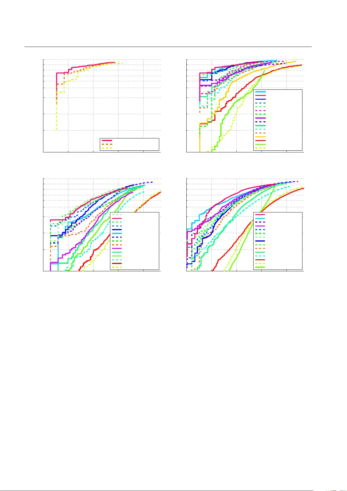
app e aring in Int. J. Comput. Vis.; c ontent may change prior to ﬁnal public ation. T raining Eﬀectiv e No de Classiﬁers for Cascade Classiﬁcation Ch unhua Shen · P eng W ang · Sakrap ee P aisitkriangkrai · An ton v an den Hengel December 2012 Abstract Cascade classiﬁers are widely used in real- time ob ject detection. Diﬀerent from conv entional clas- siﬁers that are designed for a low o verall classiﬁcation error rate, a classiﬁer in each no de of the cascade is required to achiev e an extremely high detection rate and moderate false p ositiv e rate. Although there are a few reported metho ds addressing this requirement in the context of ob ject detection, there is no princi- pled feature selection metho d that explicitly takes into accoun t this asymmetric no de learning ob jective. W e pro vide suc h an algorithm here. W e show that a spe- cial case of the biased minimax probabilit y machine has the same formulation as the linear asymmetric classiﬁer (LA C) of W u et al. ( 2005 ). W e then design a new b oost- ing algorithm that directly optimizes the cost function of LA C. The resulting totally-corrective b o osting algo- rithm is implemented by the column generation tech- nique in conv ex optimization. Experimental results on ob ject detection v erify the eﬀectiveness of the proposed b oosting algorithm as a no de classiﬁer in cascade ob- ject detection, and show p erformance better than that of the current state-of-the-art. Keyw ords AdaBo ost · Minimax Probability Ma- c hine · Cascade Classiﬁer · Ob ject Detection · Human Detection C. Shen (  ) · P . W ang · S. P aisitkriangkrai · A. v an den Hen- gel Australian Centre for Visual T echnologies, and School of Computer Science, The Universit y of Adelaide, SA 5005, Aus- tralia E-mail: chunhua.shen@adelaide.edu.au This w ork was in part supp orted by Australian Research Council F uture F ello wship FT120100969. 1 Introduction Real-time ob ject detection inherently in volv es searc h- ing a large num b er of candidate image regions for a small num b er of ob jects. Pro cessing a single image, for example, can require the interrogation of w ell ov er a million scanned windows in order to uncov er a single correct detection. This im balance in the data has an impact on the wa y that detectors are applied, but also on the training pro cess. This impact is reﬂected in the need to identify discriminativ e features from within a large ov er-complete feature set. Cascade classiﬁers ha ve b een prop osed as a poten- tial solution to the problem of im balance in the data (Viola and Jones 2004 ; Bi et al. 2006 ; Dundar and Bi 2007 ; Brubaker et al. 2008 ; W u et al. 2008 ), and ha ve receiv ed signiﬁcant atten tion due to their speed and ac- curacy . In this w ork, we prop ose a principled method b y which to train a b o osting -based cascade of classiﬁers. The b oosting-based cascade approach to ob ject de- tection was introduced b y Viola and Jones (Viola and Jones 2004 ; 2002 ), and has received signiﬁcan t subse- quen t attention (Li and Zhang 2004 ; Pham and Cham 2007b ; Pham et al. 2008 ; P aisitkriangkrai et al. 2008 ; Shen et al. 2008 ; P aisitkriangkrai et al. 2009 ). It also underpins the current state-of-the-art (W u et al. 2005 ; 2008 ). The Viola and Jones approach uses a cascade of increasingly complex classiﬁers, eac h of which aims to ac hieve the b est p ossible classiﬁcation accuracy while ac hieving an extremely lo w false negative rate. These classiﬁers can b e seen as forming the no des of a de- generate binary tree (see Fig. 1 ) whereb y a negative result from any single suc h no de classiﬁer terminates the interrogation of the current patch. Viola and Jones use AdaBoost to train each no de classiﬁer in order to 2 Ch unhua Shen et al. ac hieve the b est p ossible classiﬁcation accuracy . A low false negative rate is achiev ed by subsequently adjust- ing the decision threshold un til the desired false nega- tiv e rate is ac hieved. This process cannot be guaran teed to pro duce the b est detection performance for a giv en false negative rate. Under the assumption that each no de of the cas- cade classiﬁer makes independent classiﬁcation errors, the detection rate and false p ositive rate of the entire cascade are: F dr = Q N t =1 d t and F fp = Q N t =1 f t , resp ec- tiv ely , where d t represen ts the detection rate of classi- ﬁer t , f t the corresponding false positive rate and N the n umber of no des. As p ointed out in (Viola and Jones 2004 ; W u et al. 2005 ), these tw o equations suggest a no de le arning obje ctive : Eac h node should hav e an ex- tremely high detection rate d t ( e.g. , 99 . 7%) and a mo d- erate false p ositive rate f t ( e.g. , 50%). With the ab ov e v alues of d t and f t , and a cascade of N = 20 nodes, then F dr ≈ 94% and F fp ≈ 10 − 6 , which is a t ypical design goal. One dra wback of the standard AdaBo ost approach to b o osting is that it do es not take adv an tage of the cas- cade classiﬁer’s sp ecial structure. AdaBo ost only mini- mizes the o verall classiﬁcation error and do es not par- ticularly minimize the n umber of false negativ es. In this sense, the features selected by AdaBo ost are not opti- mal for the purp ose of rejecting as many negative ex- amples as possible. Viola and Jones prop osed a solu- tion to this problem in AsymBo ost (Viola and Jones 2002 ) (and its v ariants (Pham and Cham 2007b ; Pham et al. 2008 ; Wang et al. 2012 ; Masnadi-Shirazi and V as- concelos 2007 )) by modifying the loss function so as to more greatly penalize false negativ es. AsymBo ost ac hieves better detection rates than AdaBoost, but still addresses the no de learning goal indir e ctly , and cannot b e guaranteed to achiev e the optimal solution. W u et al. explicitly studied the no de learning goal and prop osed to use linear asymmetric classiﬁer (LAC) and Fisher linear discriminant analysis (LDA) to adjust the w eights on a set of features selected by AdaBo ost or AsymBoost (W u et al. 2005 ; 2008 ). Their experi- men ts indicated that with this p ost-pro cessing tec h- nique the no de learning ob jective can be b etter met, whic h is translated into impro v ed detection rates. In Viola and Jones’ framework, b o osting is used to select features and at the same time to train a strong classiﬁer. W u et al.’s work separates these t wo tasks: AdaBo ost or AsymBo ost is used to select features; and as a sec- ond step, LA C or LDA is used to construct a strong classiﬁer by adjusting the w eights of the selected fea- tures. The no de learning ob jective is only considered at the second step. A t the ﬁrst step—feature selection— the no de learning ob jective is not explicitly considered at all. W e conjecture that further impr ovement may b e gaine d if the no de le arning obje ctive is explicitly taken into ac c ount at b oth steps . W e thus prop ose new b o ost- ing algorithms to implemen t this idea and v erify this conjecture. A preliminary v ersion of this w ork w as pub- lished in Shen et al. ( 2010 ). Our ma jor contributions are as follo ws. 1. Starting from the theory of minimax probability mac hines (MPMs), w e deriv e a simpliﬁed version of the biased minimax probability machine, whic h has the same formulation as the linear asymmet- ric classiﬁer of W u et al. ( 2005 ). W e thus show the underlying connection b etw een MPM and LA C. Im- p ortan tly , this new interpretation w eakens some of the restrictions on the acceptable input data distri- bution imp osed by LAC. 2. W e dev elop new bo osting-like algorithms b y directly minimizing the ob jective function of the linear asym- metric classiﬁer, which results in an algorithm that w e lab el LA CBo ost. W e also prop ose FisherBo ost on the basis of Fisher LDA rather than LA C. Both metho ds may b e used to iden tify the feature set that optimally ac hiev es the no de learning goal when training a cascade classiﬁer. T o our knowledge, this is the ﬁrst attempt to design suc h a feature selection metho d. 3. LACBoost and FisherBo ost share similarities with LPBo ost (Demiriz et al. 2002 ) in the sense that both use column generation—a tec hnique originally pro- p osed for large-scale linear programming (LP). Typ- ically , the Lagrange dual problem is solved at eac h iteration in column generation. W e instead solve the primal quadratic programming (QP) problem, whic h has a sp ecial structure and entropic gradient (EG) can b e used to solve the problem v ery eﬃ- cien tly . Compared with general interior-point based QP solvers, EG is muc h faster. 4. W e apply LACBoost and FisherBo ost to ob ject de- tection and b etter p erformance is observ ed ov er oth- er metho ds (W u et al. 2005 ; 2008 ; Ma ji et al. 2008 ). In particular on p edestrian detection, FisherBo ost ac hieves the state-of-the-art, comparing with meth- o ds listed in (Doll´ ar et al. 2012 ) on three b ench- mark datasets. The results conﬁrm our conjecture and sho w the eﬀectiv eness of LA CBo ost and Fisher- Bo ost. These metho ds can b e immediately applied to other asymmetric classiﬁcation problems. Moreo ver, w e analyze the condition that makes the v alidit y of LA C, and sho w that the multi-exit cascade migh t b e more suitable for applying LAC learning of W u et al. ( 2005 ) and W u et al. ( 2008 ) (and our LAC- Bo ost) rather than Viola-Jones’ conv entional cascade. T raining Eﬀective Node Classiﬁers for Cascade Classiﬁcation 3 As observ ed in W u et al. ( 2008 ), in man y cases, LD A ev en p erforms better than LA C. In our experiments, we ha ve also observ ed similar phenomena. P aisitkriangkrai et al. ( 2009 ) empirically show ed that LDA’s criterion can b e used to ac hieve b etter detection results. An ex- planation of wh y LDA works so well for ob ject detection is missing in the literature. Here w e demonstrate that in the context of ob ject detection, LDA can b e seen as a regularized version of LAC in appro ximation. The proposed LA CBo ost/FisherBo ost algorithm dif- fers from traditional bo osting algorithms in that it do es not minimize a loss function. This op ens new p ossibil- ities for designing bo osting-lik e algorithms for sp ecial purp oses. W e hav e also extended column generation for optimizing nonlinear optimization problems. Next w e review related work in the context of real-time ob ject detection using cascade classiﬁers. 1.1 Related W ork The ﬁeld of ob ject detection has made a signiﬁcant progress ov er the last decade, esp ecially after the sem- inal work of Viola and Jones. Three key comp onents that contribute to their ﬁrst robust r e al-time ob ject de- tection framework are: 1. The cascade classiﬁer, which eﬃciently ﬁlters out negativ e patches in early no des while maintaining a v ery high detection rate; 2. AdaBo ost that selects informative features and at the same time trains a strong classiﬁer; 3. The use of integral images, whic h makes the com- putation of Haar features extremely fast. This approac h has receiv ed signiﬁcant subsequent at- ten tion. A num b er of alternativ e cascades ha ve been de- v elop ed including the soft cascade (Bourdev and Brandt 2005 ), W aldBo ost (So chman and Matas 2005 ), the dy- namic cascade (Xiao et al. 2007 ), the AND-OR cascade (Dundar and Bi 2007 ), the m ulti-exit cascade (Pham et al. 2008 ), the join t cascade (Lefakis and Fleuret 2010 ) and recently prop osed, the rate constrain t em b edded cascade (R CECBo ost) (Saberian and V asconcelos 2012 ). In this work w e hav e adopted the multi-exit cascade of Pham et al. due to its eﬀectiveness and eﬃciency as demonstrated in Pham et al. ( 2008 ). The m ulti-exit cas- cade improv es classiﬁcation p erformance by using the results of all of the weak classiﬁers applied to a patc h so far in reaching a decision at eac h node of the tree (see Fig. 1 ). Thus the n -th no de classiﬁer uses the re- sults of the weak classiﬁers asso ciated with no de n , but also those asso ciated with the previous n − 1 node clas- siﬁers in the cascade. W e sho w b elow that LAC p ost- pro cessing can enhance the m ulti-exit cascade, and that the multi-exit cascade more accurately fulﬁlls the LAC requiremen t that the margin be drawn from a Gaussian distribution. In addition to impro ving the cascade structure, a n umber of improv emen ts ha ve b een made on the learn- ing algorithm for building no de classiﬁers in a cascade. W u et al., for example, use fast forward feature selection to accelerate the training pro cedure (W u et al. 2003 ). W u et al. ( 2005 ) also show ed that LAC ma y b e used to deliver b etter classiﬁcation p erformance. Pham and Cham recently prop osed online asymmetric b o osting that considerably reduces the training time required (Pham and Cham 2007b ). By exploiting the feature statistics, Pham and Cham ( 2007a ) hav e also designed a fast method to train weak classiﬁers. Li and Zhang ( 2004 ) prop osed FloatBo ost, which discards redundan t w eak classiﬁers during AdaBoost’s greedy selection pro- cedure. Masnadi-Shirazi and V asconcelos ( 2011 ) pro- p osed cost-sensitive b o osting algorithms which can be applied to diﬀerent cost-sensitive losses b y means of gradien t descen t. Liu and Sh um ( 2003 ) also prop osed KLBo ost, aiming to select features that maximize the pro jected Kullbac k-Leibler divergence and select fea- ture w eigh ts b y minimizing the classiﬁcation error. Pro- mising results hav e also b een rep orted by LogitBo ost (T uzel et al. 2008 ) that employs the logistic regression loss, and Gen tleBo ost (T orralba et al. 2007 ) that uses adaptiv e Newton steps to ﬁt the additive model. Multi- instance b o osting has b een introduced to ob ject detec- tion (Viola et al. 2005 ; Doll´ ar et al. 2008 ; Lin et al. 2009 ), whic h do es not require precisely labeled lo ca- tions of the targets in training data. New features ha ve also been designed for improv- ing the detection p erformance. Viola and Jones’ Haar features are not suﬃciently discriminativ e for detecting more complex ob jects like p edestrians, or m ulti-view faces. Co v ariance features (T uzel et al. 2008 ) and his- togram of oriented gradients (HOG) (Dalal and T riggs 2005 ) hav e b een prop osed in this context, and eﬃcien t implemen tation approaches (along the lines of integral images) are developed for each. Shap e context, whic h can also exploit integral images (Alda vert et al. 2010 ), w as applied to human detection in thermal images (Wa- ng et al. 2010 ). The lo cal binary pattern (LBP) descrip- tor and its v arian ts ha ve b een sho wn promising per- formance on h uman detection (Mu et al. 2008 ; Zheng et al. 2010 ). Recen tly , eﬀort has b een sp en t on com- bining complementary features, including: simple con- catenation of HOG and LBP (Wang et al. 2007 ), com- bination of heterogeneous local features in a bo osted cascade classiﬁer (W u and Nev atia 2008 ), and Bay esian in tegration of intensit y , depth and motion features in a mixture-of-exp erts mo del (Enzweiler et al. 2010 ). 4 Ch unhua Shen et al. 1 2 N F F F T T T T input target h 1 , h 2 , · · · h j , h j +1 , · · · · · · , h n − 1 , h n 1 2 N F F F T T T T input target h 1 , h 2 , · · · h j , h j +1 , · · · · · · , h n − 1 , h n Fig. 1: Cascade classiﬁers. The ﬁrst one is the standard cascade of Viola and Jones ( 2004 ). The second one is the m ulti-exit cascade prop osed in Pham et al. ( 2008 ). Only those classiﬁed as true detection by all no des will b e true targets. The rest of the pap er is organized as follows. W e brieﬂy review the concept of minimax probabilit y ma- c hine and derive the new simpliﬁed version of biased minimax probabilit y mac hine in Section 2 . Linear asym- metric classiﬁcation and its connection to the minimax probabilit y machine is discussed in Section 3 . In Sec- tion 4 , we show ho w to design new b o osting algorithms (LA CBo ost and FisherBo ost) b y rewriting the opti- mization form ulations of LA C and Fisher LD A. The new b o osting algorithms are applied to ob ject detec- tion in Section 5 and we conclude the pap er in Section 6 . 1.2 Notation The follo wing notation is used. A matrix is denoted b y a b old upp er-case letter ( X ); a column vector is denoted b y a b old lo wer-case letter ( x ). The i th row of X is denoted by X i : and the i th column X : i . The identit y matrix is I and its size should be clear from the con text. 1 and 0 are column vectors of 1’s and 0’s, resp ectively . W e use < , 4 to denote comp onent-wise inequalities. Let T = { ( x i , y i ) } i =1 , ··· ,m b e the set of training data, where x i ∈ X and y i ∈ {− 1 , +1 } , ∀ i . The train- ing set consists of m 1 p ositiv e training p oints and m 2 negativ e ones; m 1 + m 2 = m . Let h ( · ) ∈ H be a w eak classiﬁer that pro jects an input vector x in to {− 1 , +1 } . Note that here w e consider only classiﬁers with discrete outputs although the developed metho ds can use real- v alued weak classiﬁers to o. W e assume that H , the set from whic h h ( · ) is selected, is ﬁnite and has n elemen ts. Deﬁne the matrix H Z ∈ R m × n suc h that the ( i, j ) en try H Z ij = h j ( x i ) is the lab el predicted b y weak clas- siﬁer h j ( · ) for the datum x i , where x i the i th elemen t of the set Z . In order to simplify the notation we eliminate the sup erscript when Z is the training set, so H Z = H . Therefore, eac h column H : j of the matrix H consists of the output of w eak classiﬁer h j ( · ) on all the train- ing data; while each row H i : con tains the outputs of all w eak classiﬁers on the training datum x i . Deﬁne simi- larly the matrix A ∈ R m × n suc h that A ij = y i h j ( x i ). Note that b o osting algorithms entirely dep ends on the matrix A and do not directly in teract with the train- ing examples. Our following discussion will thus largely fo cus on the matrix A . W e write the vector obtained b y m ultiplying a matrix A with a vector w as Aw and its i th entry as ( Aw ) i . If we let w represen t the co- eﬃcien ts of a selected weak classiﬁer then the margin of the training datum x i is ρ i = A i : w = ( Aw ) i and the vector of suc h margins for all of the training data is ρ = Aw . 2 Minimax Probabilit y Mac hines Before w e in tro duce our b o osting algorithm, let us brieﬂy review the concept of minimax probability machines (MPM) (Lanckriet et al. 2002 ) ﬁrst. 2.1 Minimax Probability Classiﬁers Let x 1 ∈ R n and x 2 ∈ R n denote tw o random v ectors dra wn from tw o distributions with means and cov ari- T raining Eﬀective Node Classiﬁers for Cascade Classiﬁcation 5 ances ( µ 1 , Σ 1 ) and ( µ 2 , Σ 2 ), respectively . Here µ 1 , µ 2 ∈ R n and Σ 1 , Σ 2 ∈ R n × n . W e deﬁne the class lab els of x 1 and x 2 as +1 and − 1, w.l.o.g. The minimax probabilit y mac hine (MPM) seeks a robust separation h yp erplane that can separate the tw o classes of data with the max- imal probability . The h yp erplane can b e expressed as w > x = b with w ∈ R n \{ 0 } and b ∈ R . The problem of iden tifying the optimal hyperplane ma y then b e formu- lated as max w ,b,γ γ s . t .  inf x 1 ∼ ( µ 1 , Σ 1 ) Pr { w > x 1 ≥ b }  ≥ γ , (1)  inf x 2 ∼ ( µ 2 , Σ 2 ) Pr { w > x 2 ≤ b }  ≥ γ . Here γ is the low er b ound of the classiﬁcation accuracy (or the w orst-case accuracy) on test data. This problem can be transformed into a conv ex problem, more specif- ically a second-order cone program (SOCP) (Boyd and V andenberghe 2004 ) and thus can b e solved eﬃciently (Lanc kriet et al. 2002 ). 2.2 Biased Minimax Probability Machines The form ulation ( 1 ) assumes that the classiﬁcation prob- lem is balanced. It attempts to ac hieve a high recog- nition accuracy , which assumes that the losses asso ci- ated with all mis-classiﬁcations are identical. How ev er, in many applications this is not the case. Huang et al. ( 2004 ) prop osed a biased v ersion of MPM through a slight mo diﬁcation of ( 1 ), which may b e formulated as max w ,b,γ γ s . t .  inf x 1 ∼ ( µ 1 ,Σ 1 ) Pr { w > x 1 ≥ b }  ≥ γ , (2)  inf x 2 ∼ ( µ 2 ,Σ 2 ) Pr { w > x 2 ≤ b }  ≥ γ ◦ . Here γ ◦ ∈ (0 , 1) is a prescribed constan t, which is the acceptable classiﬁcation accuracy for the less important class. The resulting decision h yp erplane prioritizes the classiﬁcation of the imp ortant class x 1 o ver that of the less imp ortant class x 2 . Biased MPM is thus exp ected to p erform b etter in biased classiﬁcation applications. Huang et al. sho wed that ( 2 ) can b e iterativ ely solv ed via solving a sequence of SOCPs using the fractional programming (FP) technique. Clearly it is signiﬁcantly more computationally demanding to solve ( 2 ) than ( 1 ). Next w e sho w how to re-form ulate ( 2 ) in to a simpler quadratic program (QP) based on the recen t theoretical results in (Y u et al. 2009 ). 2.3 Simpliﬁed Biased Minimax Probability Machines In this section, w e are in terested in simplifying the prob- lem of ( 2 ) for a special case of γ ◦ = 0 . 5, due to its imp ortan t application in ob ject detection (Viola and Jones 2004 ; W u et al. 2005 ). In the following discus- sion, for simplicity , we only consider γ ◦ = 0 . 5 although some algorithms developed may also apply to γ ◦ < 0 . 5. Theoretical results in (Y u et al. 2009 ) sho w that, the w orst-case constraint in ( 2 ) can b e written in diﬀerent forms when x follows arbitrary , symmetric, symmetric unimo dal or Gaussian distributions (see Appendix A ). Both the MPM (Lanc kriet et al. 2002 ) and the biased MPM (Huang et al. 2004 ) are based the most general form of the four cases sho wn in Appendix A , i.e. , Equa- tion ( 27 ) for arbitrary distributions, as they do not im- p ose constraints up on the distributions of x 1 and x 2 . Ho wev er, one may take adv an tage of structural in- formation whenever av ailable. F or example, it is shown in (W u et al. 2005 ) that, for the face detection problem, w eak classiﬁer outputs can b e w ell appro ximated b y the Gaussian distribution. In other w ords, the constraint for arbitrary distributions does not utilize any t yp e of a priori information, and hence, for many problems, con- sidering arbitrary distributions for simplifying ( 1 ) and ( 2 ) is to o c onservative . Since b oth the MPM (Lanckriet et al. 2002 ) and the biased MPM (Huang et al. 2004 ) do not assume any constraints on the distribution family , they fail to exploit this structural information. Let us consider the special case of γ ◦ = 0 . 5. It is easy to see that the w orst-case constrain t in ( 2 ) b ecomes a simple linear constraint for symmetric, symmetric uni- mo dal, as well as Gaussian distributions (see App endix A ). As p ointed out in (Y u et al. 2009 ), such a result is the immediate consequence of symmetry b ecause the w orst-case distributions are forced to put probabilit y mass arbitrarily far aw a y on b oth sides of the mean. In such case, an y information ab out the cov ariance is neglected. W e now apply this result to the biased MPM as represen ted b y ( 2 ). Our main result is the following theorem. Theorem 1 With γ ◦ = 0 . 5 , the biase d minimax pr ob- lem ( 2 ) c an b e formulate d as an unc onstr aine d pr oblem: max w w > ( µ 1 − µ 2 ) p w > Σ 1 w , (3) under the assumption that x 2 fol lows a symmetric dis- tribution. The optimal b c an b e obtaine d thr ough: b = w > µ 2 . (4) 6 Ch unhua Shen et al. The worst-c ase classiﬁc ation ac cur acy for the ﬁrst class, γ ? , is obtaine d by solving ϕ ( γ ? ) = − b ? + a ? > µ 1 p w ? > Σ 1 w ? , (5) wher e ϕ ( γ ) =              q γ 1 − γ if x 1 ∼ ( µ 1 , Σ 1 ) , q 1 2(1 − γ ) if x 1 ∼ ( µ 1 , Σ 1 ) S , 2 3 q 1 2(1 − γ ) if x 1 ∼ ( µ 1 , Σ 1 ) SU , φ − 1 ( γ ) if x 1 ∼ G ( µ 1 , Σ 1 ) . (6) and { w ? , b ? } is the optimal solution of ( 3 ) and ( 4 ) . Please refer to App endix A for the pro of of Theorem 1 . W e hav e deriv ed the biased MPM algorithm from a diﬀeren t p ersp ective. W e reveal that only the assump- tion of symmetric distributions is needed to arrive at a simple unconstrained formulation. Compared with the approac h in (Huang et al. 2004 ), w e hav e used more information to simply the optimization problem. More imp ortan tly , as will b e sho wn in the next section, this unconstrained form ulation enables us to design a new b o osting algorithm. There is a close connection betw een our algorithm and the linear asymmetric classiﬁer (LA C) in (W u et al. 2005 ). The resulting problem ( 3 ) is exactly the same as LA C in (W u et al. 2005 ). Remo ving the inequalit y in this constrain t leads to a problem solv able b y eigen- decomp osition. W e hav e thus shown that the results of W u et al. may b e generalized from the Gaussian dis- tributions assumed in (W u et al. 2005 ) to symmetric distributions. 3 Linear Asymmetric Classiﬁcation W e hav e shown that starting from the biased minimax probabilit y machine, we are able to obtain the same optimization formulation as shown in W u et al. ( 2005 ), while m uch weak ening the underlying assumption (sym- metric distributions v ersus Gaussian distributions). Be- fore w e prop ose our LACBoost and FisherBo ost, how- ev er, w e pro vide a brief ov erview of LAC. W u et al. ( 2008 ) prop osed linear asymmetric clas- siﬁcation (LAC) as a p ost-pro cessing step for training no des in the cascade framework. In (W u et al. 2008 ), it is stated that LA C is guaranteed to reach an optimal solution under the assumption of Gaussian data distri- butions. W e now kno w that this Gaussianalit y condition ma y b e relaxed. Supp ose that we hav e a linear classiﬁer f ( x ) = sign ( w > x − b ) . W e seek a { w , b } pair with a v ery high accuracy on the p ositiv e data x 1 and a mo derate accuracy on the nega- tiv e x 2 . This can be expressed as the follo wing problem: max w 6 = 0 ,b Pr x 1 ∼ ( µ 1 , Σ 1 ) { w > x 1 ≥ b } , s . t . Pr x 2 ∼ ( µ 2 , Σ 2 ) { w > x 2 ≤ b } = λ. (7) In (W u et al. 2005 ), λ is set to 0 . 5 and it is assumed that for any w , w > x 1 is Gaussian and w > x 2 is sym- metric, ( 7 ) can b e approximated b y ( 3 ). Again, these assumptions ma y b e relaxed as w e hav e shown in the last section. Problem ( 3 ) is similar to LDA’s optimiza- tion problem max w 6 = 0 w > ( µ 1 − µ 2 ) p w > ( Σ 1 + Σ 2 ) w . (8) Problem ( 3 ) can b e solved by eigen-decomp osition and a closed-form solution can b e derived: w ? = Σ − 1 1 ( µ 1 − µ 2 ) , b ? = w ? > µ 2 . (9) On the other hand, each node in cascaded bo osting clas- siﬁers has the following form: f ( x ) = sign ( w > H ( x ) − b ) . (10) W e ov erride the sym b ol H ( x ) here, which denotes the output vector of all weak classiﬁers o ver the datum x . W e can cast each no de as a linear classiﬁer o ver the feature space constructed by the binary outputs of all w eak classiﬁers. F or each node in a cascade classiﬁer, w e wish to maximize the detection rate while main taining the false p ositive rate at a mo derate level (for example, around 50 . 0%). That is to sa y , the problem ( 3 ) repre- sen ts the no de learning goal. Bo osting algorithms such as AdaBo ost can b e used as feature selection metho ds, and LA C is used to learn a linear classiﬁer o ver those bi- nary features c hosen b y b o osting as in W u et al. ( 2005 ). The adv an tage of this approach is that LAC considers the asymmetric no de learning explicitly . Ho wev er, there is a precondition on the v alidity of LA C that for any w , w > x 1 is a Gaussian and w > x 2 is symmetric. In the case of b o osting classiﬁers, w > x 1 and w > x 2 can b e expressed as the margin of positive data and negativ e data, resp ectively . Empirically W u et al. ( 2008 ) veriﬁed that w > x is approximately Gaussian for a cascade face detector. W e discuss this issue in more detail in Section 5 . Shen and Li ( 2010b ) theoretically pro ved that under the assumption that weak classiﬁers are independent, the margin of AdaBo ost follows the Gaussian distribution, as long as the num b er of w eak classiﬁers is suﬃciently lar ge . In Section 5 we v erify this theoretical result by p erforming the normalit y test on no des with diﬀerent num b er of weak classiﬁers. T raining Eﬀective Node Classiﬁers for Cascade Classiﬁcation 7 4 Constructing Bo osting Algorithms from LD A and LAC In kernel metho ds, the original data are nonlinearly mapp ed to a feature space by a mapping function Ψ ( · ). The function need not b e known, how ever, as rather than b eing applied to the data directly , it acts instead through the inner product Ψ ( x i ) > Ψ ( x j ). In b o osting (R¨ atsch et al. 2002 ), ho wev er, the mapping function can be seen as being explicitly kno wn, as Ψ ( x ) : x 7→ [ h 1 ( x ) , . . . , h n ( x )] . Let us consider the Fisher LDA case ﬁrst b ecause the solution to LDA will generalize to LA C straigh tforwardly , by lo oking at the similarity b etw een ( 3 ) and ( 8 ). Fisher LD A maximizes the b etw een-class v ariance and minimizes the within-class v ariance. In the binary- class case, the more general form ulation in ( 8 ) can be expressed as max w ( µ 1 − µ 2 ) 2 σ 1 + σ 2 = w > C b w w > C w w , (11) where C b and C w are the betw een-class and within- class scatter matrices; µ 1 and µ 2 are the pro jected cen ters of the tw o classes. The ab ov e problem can b e equiv alen tly reformulated as min w w > C w w − θ ( µ 1 − µ 2 ) , (12) for some certain constan t θ and under the assumption that µ 1 − µ 2 ≥ 0. 1 No w in the feature space, our data are Ψ ( x i ), i = 1 . . . m . Deﬁne the v ectors e , e 1 , e 2 ∈ R m suc h that e = e 1 + e 2 , the i -th en try of e 1 is 1 /m 1 if y i = +1 and 0 otherwise, and the i -th entry of e 2 is 1 /m 2 if y i = − 1 and 0 otherwise. W e then see that µ 1 = 1 m 1 w > X y i =1 Ψ ( x i ) = 1 m 1 X y i =1 A i : w = 1 m 1 X y i =1 ( Aw ) i = e > 1 Aw , (13) and µ 2 = 1 m 2 w > X y i = − 1 Ψ ( x i ) = 1 m 2 X y i = − 1 H i : w = − e > 2 Aw , (14) F or ease of exp osition w e order the training data ac- cording to their lab els so the v ector e ∈ R m : e = [1 /m 1 , · · · , 1 /m 2 , · · · ] > , (15) and the ﬁrst m 1 comp onen ts of ρ corresp ond to the p os- itiv e training data and the remaining ones corresp ond 1 In our ob ject detection exp eriment, w e found that this assumption can alwa ys b e satisﬁed. to the m 2 negativ e data. W e no w see that µ 1 − µ 2 = e > ρ , C w = m 1 /m · Σ 1 + m 2 /m · Σ 2 with Σ 1 , 2 the co v ariance matrices. Noting that w > Σ 1 , 2 w = 1 m 1 , 2 ( m 1 , 2 − 1) X i>k,y i = y k = ± 1 ( ρ i − ρ k ) 2 , w e can easily rewrite the original problem ( 11 ) (and ( 12 )) into: min w , ρ 1 2 ρ > Q ρ − θ e > ρ , s . t . w < 0 , 1 > w = 1 , ρ i = ( Aw ) i , i = 1 , · · · , m. (16) Here Q =  Q 1 0 0 Q 2  is a blo ck matrix with Q 1 =       1 m − 1 m ( m 1 − 1) . . . − 1 m ( m 1 − 1) − 1 m ( m 1 − 1) 1 m . . . − 1 m ( m 1 − 1) . . . . . . . . . . . . − 1 m ( m 1 − 1) − 1 m ( m 1 − 1) . . . 1 m       , and Q 2 is similarly deﬁned by replacing m 1 with m 2 in Q 1 : Q 2 =       1 m − 1 m ( m 2 − 1) . . . − 1 m ( m 2 − 1) − 1 m ( m 2 − 1) 1 m . . . − 1 m ( m 2 − 1) . . . . . . . . . . . . − 1 m ( m 2 − 1) − 1 m ( m 2 − 1) . . . 1 m       . Also note that w e hav e introduced a constant 1 2 b efore the quadratic term for conv enience. The normalization constrain t 1 > w = 1 remo v es the scale am biguity of w . Without it the problem is ill-p osed. W e see from the form of ( 3 ) that the cov ariance of the negativ e data is not in volv ed in LAC and th us that if w e set Q =  Q 1 0 0 0  then ( 16 ) b ecomes the optimization problem of LAC. A t this stage, it remains unclear ab out how to solve the problem ( 16 ) b ecause w e do not know all the weak classiﬁers. There may b e extremely (or ev en inﬁnitely) man y weak classiﬁers in H , the set from which h ( · ) is selected, meaning that the dimension of the optimiza- tion v ariable w may also b e extremely large. So ( 16 ) is a semi-inﬁnite quadratic program (SIQP). W e sho w ho w column generation can b e used to solve this prob- lem. T o make column generation applicable, w e need to deriv e a sp eciﬁc Lagrange dual of the primal problem. 8 Ch unhua Shen et al. 4.1 The Lagrange Dual Problem W e no w deriv e the Lagrange dual of the quadratic prob- lem ( 16 ). Although we are only interested in the v ari- able w , w e need to keep the auxiliary v ariable ρ in order to obtain a meaningful dual problem. The Lagrangian of ( 16 ) is L ( w , ρ | {z } primal , u , r |{z} dual ) = 1 2 ρ > Q ρ − θ e > ρ + u > ( ρ − Aw ) − q > w + r ( 1 > w − 1) , (17) with q < 0 . sup u ,r inf w , ρ L ( w , ρ , u , r ) gives the follow- ing Lagrange dual: max u ,r − r − regularization z }| { 1 2 ( u − θ e ) > Q − 1 ( u − θ e ) , s . t . m X i =1 u i A i : 4 r 1 > . (18) In our case, Q is rank-deﬁcient and its in verse does not exist (for b oth LD A and LAC). Actually for b oth Q 1 and Q 2 , they ha ve a zero eigen v alue with the cor- resp onding eigenv ector b eing all ones. This is easy to see because for Q 1 and Q 2 , the sum of each row (or eac h column) is zero. W e can simply regularize Q with Q + ˜ δ I with ˜ δ a small p ositiv e constant. Actually , Q is a diagonally dominant matrix but not strict diagonal dominance. So Q + ˜ δ I with an y ˜ δ > 0 is strict diago- nal dominance and by the Gershgorin circle theorem, a strictly diagonally dominant matrix must b e inv ertible. One of the KKT optimality conditions b etw een the dual and primal is ρ ? = − Q − 1 ( u ? − θ e ) , (19) whic h can b e used to establish the connection b etw een the dual optimum and the primal optimum. This is ob- tained by the fact that the gradient of L w.r.t. ρ m ust v anish at the optimum, ∂ L/∂ ρ i = 0, ∀ i = 1 · · · n . Problem ( 18 ) can b e viewed as a regularized LP- Bo ost problem. Compared with the hard-margin LP- Bo ost (Demiriz et al. 2002 ), the only diﬀerence is the regularization term in the cost function. The duality gap b etw een the primal ( 16 ) and the dual ( 18 ) is zero. In other w ords, the solutions of ( 16 ) and ( 18 ) coincide. Instead of solving ( 16 ) directly , one calculates the most violated constrain t in ( 18 ) iterativ ely for the current solution and adds this constrain t to the optimization problem. In theory , an y column that violates dual fea- sibilit y can b e added. T o sp eed up the con vergence, we add the most violated constrain t by solving the follow- ing problem: h 0 ( · ) = argmax h ( · ) m X i =1 u i y i h ( x i ) . (20) This is exactly the same as the one that standard Ad- aBo ost and LPBo ost use for producing the best weak classiﬁer at each iteration. That is to say , to ﬁnd the w eak classiﬁer that has the minimum weigh ted train- ing error. W e summarize the LACBoost/FisherBo ost algorithm in Algorithm 1 . By simply c hanging Q 2 , Al- gorithm 1 can be used to train either LACBoost or FisherBo ost. Note that to obtain an actual strong clas- siﬁer, one may need to include an oﬀset b , i.e. the ﬁnal classiﬁer is P n j =1 h j ( x ) − b b ecause from the cost func- tion of our algorithm ( 12 ), w e can see that the cost function itself do es not minimize an y classiﬁcation er- ror. It only ﬁnds a pro jection direction in whic h the data can b e maximally separated. A simple line search can ﬁnd an optimal b . Moreov er, when training a cas- cade, we need to tune this oﬀset an ywa y as shown in ( 10 ). The conv ergence of Algorithm 1 is guaranteed by general column generation or cutting-plane algorithms, whic h is easy to establish: Theorem 2 The c olumn gener ation pr o c e dur e de cr e ases the obje ctive value of pr oblem ( 16 ) at e ach iter ation and henc e in the limit it solves the pr oblem ( 16 ) glob al ly to a desir e d ac cur acy. The proof is deferred to App endix B . In short, when a new h 0 ( · ) that violates dual feasibilit y is added, the new optimal v alue of the dual problem (maximization) w ould decrease. Accordingly , the optimal v alue of its primal problem decreases to o b ecause they hav e the same optimal v alue due to zero dualit y gap. Moreo ver the primal cost function is conv ex, therefore in the end it conv erges to the global minimum. A t each iteration of column generation, in theory , w e can solve either the dual ( 18 ) or the primal problem ( 16 ). Here we choose to solv e an equiv alent v ariant of the primal problem ( 16 ): min w 1 2 w > ( A > QA ) w − ( θ e > A ) w , s . t . w ∈ ∆ n , (21) where ∆ n is the unit simplex, which is deﬁned as { w ∈ R n : 1 > w = 1 , w < 0 } . In practice, it could b e m uch faster to solve ( 21 ) since 1. Generally , the primal problem has a smaller size, hence faster to solve. The n umber of v ariables of ( 18 ) is m at each iteration, while the num b er of v ariables is the num b er of iterations for the primal T raining Eﬀective Node Classiﬁers for Cascade Classiﬁcation 9 Algorithm 1 Column generation for SIQP . Input : Lab eled training data ( x i , y i ) , i = 1 · · · m ; termina- tion threshold ε > 0; regularization parameter θ ; maximum num b er of iterations n max . Initialization : m = 0; w = 0 ; and u i = 1 m , i = 1 · · · m . 1 for iteration = 1 : n max do 2 − Check for the optimality: 3 if iteration > 1 and P m i =1 u i y i h 0 ( x i ) < r + ε , then break; and the problem is solved; − Add h 0 ( · ) to the restricted master problem, which 4 corresponds to a new constrain t in the dual; − Solve the dual problem ( 18 ) (or the primal problem 5 ( 16 )) and up date r and u i ( i = 1 · · · m ). − Incremen t the num b er of w eak classiﬁers n = n + 1. 6 Output : The selected features are h 1 , h 2 , . . . , h n . The ﬁ- nal strong classiﬁer is: F ( x ) = P n j =1 w j h j ( x ) − b . Here the oﬀset b can b e learned b y a simple line search . problem. F or example, in Viola-Jones’ face detection framew ork, the n umber of training data m = 10 , 000 and n max = 200. In other w ords, the primal problem has at most 200 v ariables in this case; 2. The dual problem ( 18 ) is a standard QP problem. It has no sp ecial structure to exploit. As w e will sho w, the primal problem ( 21 ) b elongs to a sp ecial class of problems and can b e eﬃcient ly solved us- ing en tropic/exponentiated gradien t descen t (EG) (Bec k and T eb oulle 2003 ; Collins et al. 2008 ). See App endix C for details of the EG algorithm. A fast QP solv er is extremely imp ortant for training our ob ject detector since w e need to solve a few thousand QP problems. Compared with standard QP solvers like Mosek (MOSEK 2010 ), EG is muc h faster. EG mak es it p ossible to train a detector using almost the same amoun t of time as using standard AdaBo ost b ecause the ma jority of time is sp ent on w eak classiﬁer training and b o otstrapping. W e can reco v er b oth of the dual v ariables u ? , r ? eas- ily from the primal v ariable w ? , ρ ? : u ? = − Q ρ ? + θ e ; (22) r ? = max j =1 ...n  P m i =1 u ? i A ij  . (23) The second equation is obtained by the fact that in the dual problem’s constrain ts, at optim um, there m ust exist at least one u ? i suc h that the equality holds. That is to sa y , r ? is the largest e dge o v er all weak classiﬁers. In summary , when using EG to solve the primal problem, Line 5 of Algorithm 1 is: − Solve the primal pr oblem ( 21 ) using EG, and up- date the dual variables u with ( 22 ) , and r with ( 23 ) . −0.5 0 0.5 1 1.5 0 0.5 1 1.5 x 1 x 2 −0.5 0 0.5 1 1.5 0 0.5 1 1.5 x 1 x 2 Fig. 2: Decision b oundaries of AdaBo ost (top) and FisherBo ost (bottom) on 2D artiﬁcial data generated from the Gaussian distribution (p ositive data repre- sen ted b y  ’s and negative data b y × ’s). W eak classi- ﬁers are v ertical and horizon tal decision stumps. Fisher- Bo ost emphasizes more on positive samples than neg- ativ e samples. As a result, the decision boundary of FisherBo ost is more similar to the Gaussian distribu- tion than the decision b oundary of AdaBo ost. 5 Exp eriments In this section, we p erform our exp eriments on both syn thetic and challenging real-w orld data sets, e.g. , face and p edestrian detection. 5.1 Synthetic T esting W e ﬁrst illustrate the p erformance of FisherBo ost on an asymmetrical synthetic data set where there are a large num b er of negative samples compared to the p os- itiv e ones. Fig. 2 demonstrates the subtle diﬀerence in classiﬁcation boundaries betw een AdaBo ost and Fisher- Bo ost. It can be observed that FisherBo ost places more 10 Ch unhua Shen et al. emphasis on p ositive samples than negative samples to ensure these p ositive samples w ould b e classiﬁed cor- rectly . AdaBo ost, on the other hand, treat b oth p osi- tiv e and negativ e samples equally . This might b e due to the fact that AdaBo ost only optimizes the ov erall clas- siﬁcation accuracy . This ﬁnding is consisten t with our results rep orted earlier in (Paisitkriangkrai et al. 2009 ; Shen et al. 2011 ). 5.2 Comparison With Other Asymmetric Bo osting In this exp eriment, FisherBo ost and LACBoost are com- pared against sev eral asymmetric b o osting algorithms, namely , AdaBo ost with LAC or Fisher LD A p ost-pro- cessing (W u et al. 2008 ), AsymBo ost (Viola and Jones 2002 ), cost-sensitive AdaBo ost (CS-ADA) (Masnadi- Shirazi and V asconcelos 2011 ) and rate constrained b o o- sting (RCBoost) (Sab erian and V asconcelos 2012 ). The results of AdaBo ost are also presented as the baseline. F or each algorithm, we train a strong classiﬁer consist- ing of 100 weak classiﬁers along with their co eﬃcients. The threshold w as determined such that the false p os- itiv e rate of test set is 50%. F or every method, the ex- p erimen t is repeated 5 times and the a verage detec- tion rate on p ositive class is rep orted. F or FisherBo ost and LACBoost, the parameter θ is chosen from { 1 / 10 , 1 / 12 , 1 / 15 , 1 / 20 } b y cross-v alidation. F or AsymBo ost, w e c ho ose k (asymmetric factor) from { 2 0 . 1 , 2 0 . 2 , · · · , 2 0 . 5 } b y cross-v alidation. F or CS-ADA, we set the cost for misclassifying p ositive and negative data as follows. W e assign the asymmetric factor k = C 1 /C 2 and re- strict 0 . 5( C 1 + C 2 ) = 1. W e choose k from { 1 . 2 , 1 . 65 , 2 . 1 , 2 . 55 , 3 } by cross-v alidation. F or RCBoost, we con- duct t wo exp e rimen ts. In the ﬁrst experiment, we use the same training set to enforce the target detection rate, while in the second exp eriment; w e use 75% of the training data to train the mo del and the other 25% to enforce the target detection rate. W e set the target de- tection rate, D T , to 99 . 5%, the barrier co eﬃcient, γ , to 2 and the num b er of iterations b efore halving γ , N d , to 10. W e tested the p erformance of all algorithms on ﬁve real-w orld data sets, including b oth machine learning (USPS) and vision data sets (cars, faces, p edestrians, scenes). W e categorized USPS data sets in to t wo classes: ev en digits and o dd digits. F or faces, we use face data sets from (Viola and Jones 2004 ) and randomly ex- tract 5000 negative patc hes from background images. W e apply principle comp onent analysis (PCA) to pre- serv e 95% total v ariation. The new data set has a di- mension of 93. F or UIUC car (Agarwal et al. 2004 ), we do wnsize the original image from 40 × 100 pixels to 20 × 50 pixels and apply PCA. The pro jected data capture 95% total v ariation and has a ﬁnal dimension of 228. F or Daimler-Chrysler pedestrian data sets (Munder and Ga vrila 2006 ), w e apply PCA to the original 18 × 36 pix- els. The pro jected data capture 95% v ariation and has a ﬁnal dimension of 139. F or indo or/outdo or scene, w e divide the 15-scene data set used in (Lazebnik et al. 2006 ) into 2 groups: indoor and outdo or scenes. W e use CENTRIST as our feature descriptors and build 50 visual code words using the histogram in tersection k ernel (W u and Rehg 2011 ). Each image is represented in a spatial hierarc hy manner. Eac h image consists of 31 sub-windo ws. In total, there are 1550 feature dimen- sions p er image. All 5 classiﬁers are trained to remo ve 50% of the negativ e data, while retaining almost all p os- itiv e data. W e compare their detection rates in T able 1 . F rom our exp eriments, FisherBoost demonstrates the b est performance on most data sets. How ever, LAC- Bo ost does not p erform as w ell as exp ected. W e sus- p ect that the p o or p erformance might partially due to n umerical issues, whic h can cause o verﬁtting. W e will discuss this in more detail in Section 5.6 . 5.3 F ace Detection Us ing a Cascade Classiﬁer In this experiments, eight asymmetric b o osting meth- o ds are ev aluated with the multi-exit cascade (Pham et al. 2008 ), whic h are FisherBo ost/LACBoost, Ad- aBo ost alone or with LD A/LAC p ost-pro cessing (W u et al. 2008 ), AsymBo ost alone or with LDA/LA C p ost- pro cessing. W e ha ve also implemented Viola-Jones’ face detector (AdaBo ost with the con v entional cascade) as the baseline (Viola and Jones 2004 ). F urthermore, our face detector is also compared with state-of-the-art in- cluding some cascade design metho ds, i.e. , W aldBo ost (So c hman and Matas 2005 ), FloatBo ost (Li and Zhang 2004 ), Boosting Chain (Xiao et al. 2003 ) and the exten- sion of (Sab erian and V asconcelos 2010 ), RCECBoost (Sab erian and V asconcelos 2012 ). The algorithm for training a multi-exit cascade is summarized in Algo- rithm 2 . W e ﬁrst illustrate the v alidity of adopting LAC and Fisher LDA p ost-pro cessing to improv e the no de learn- ing ob jective in the cascade classiﬁer. As described abo- v e, LAC and LD A assume that the margin of the train- ing data asso ciated with the no de classiﬁer in such a cascade exhibits a Gaussian distribution. W e demon- strate this assumption on the face detection task in Fig. 3 . Fig. 3 shows the normal probability plot of the margins of the p ositiv e training data for the ﬁrst three no de classiﬁers in the m ulti-exit LA C classiﬁer. The ﬁg- ure rev eals that the larger the n um b er of w eak classiﬁers used the more closely the margins follow the Gaussian T raining Eﬀective Node Classiﬁers for Cascade Classiﬁcation 11 AdaBoost LAC FLDA AsymBoost CS-ADA RCBoost 1 RCBoost 2 LACBoost FisherBoost Digits 99 . 30 (0 . 10) 99 . 30 (0 . 21) 99 . 37 (0 . 08) 99 . 40 ( 0 . 11 ) 99 . 37 (0 . 09) 99 . 36 (0 . 17) 99 . 27 (0 . 15) 99 . 12 (0 . 07) 99 . 40 ( 0 . 13 ) F aces 98 . 70 (0 . 14) 98 . 78 (0 . 42) 98 . 86 (0 . 22) 98 . 73 (0 . 14) 98 . 71 (0 . 20) 98 . 75 (0 . 18) 98 . 66 (0 . 23) 98 . 63 (0 . 29) 98 . 89 ( 0 . 15 ) Cars 97 . 02 (1 . 55) 97 . 07 (1 . 34) 97 . 02 (1 . 50) 97 . 11 (1 . 36) 97 . 47 (1 . 31) 96 . 84 (0 . 87) 96 . 62 (1 . 08) 96 . 80 (1 . 47) 97 . 78 ( 1 . 27 ) Pedestrians 98 . 54 (0 . 34) 98 . 59 (0 . 71) 98 . 69 (0 . 28) 98 . 55 (0 . 45) 98 . 51 (0 . 36) 98 . 67 (0 . 29) 98 . 65 (0 . 39) 99 . 12 ( 0 . 35 ) 98 . 73 (0 . 33) Scenes 99 . 59 (0 . 10) 99 . 54 (0 . 21) 99 . 57 (0 . 12) 99 . 66 (0 . 12) 99 . 68 (0 . 10) 99 . 61 (0 . 19) 99 . 62 (0 . 16) 97 . 50 (1 . 07) 99 . 66 ( 0 . 10 ) Average 98 . 63 98 . 66 98 . 70 98 . 69 98 . 75 98 . 64 98 . 56 98 . 23 98 . 89 T able 1: T est errors (%) on ﬁve real-world data sets. All exp eriments are run 5 times with 100 b o osting iterations. The a verage detection rate and standard deviation (in percentage) at 50% false positives are reported. Best av erage detection rate is shown in b oldface. −3 −2 −1 0 1 2 3 0.001 0.003 0.01 0.02 0.05 0.10 0.25 0.50 0.75 0.90 0.95 0.98 0.99 0.997 0.999 margin probablity −4 −2 0 2 4 6 0.001 0.003 0.01 0.02 0.05 0.10 0.25 0.50 0.75 0.90 0.95 0.98 0.99 0.997 0.999 margin probablity −10 −5 0 5 10 15 20 0.001 0.003 0.01 0.02 0.05 0.10 0.25 0.50 0.75 0.90 0.95 0.98 0.99 0.997 0.999 margin probablity Fig. 3: Normality test (normal probabilit y plot) for the face data’s margin distribution of no des 1, 2, 3. The 3 no des con tains 7, 22, 52 w eak classiﬁers respectively . The data are plotted against a theoretical normal distribution suc h that the data which follows the normal distribution mo del should form a straigh t line. Curves deviated from the straight line (the red line) indicate departures from normalit y . The larger the num b er of weak classiﬁers, the more closely the margin follow the Gaussian distribution. distribution. F rom this, we infer that LAC/LD A p ost- processing and th us LA CBo ost and FisherBoost, can b e exp ected to ac hieve a better performance when a larger n umber of weak c lassiﬁers are used. W e there- fore apply LAC/LD A only within the later nodes (for example, 9 onw ards) of a m ulti-exit cascade as these no des con tain more weak classiﬁers. W e choose m ulti- exit due to its property 2 and eﬀectiveness as reported in (Pham et al. 2008 ). W e ha ve compared the m ulti- exit cascade with LDA/LA C p ost-processing against the conv entional cascade with LD A/LAC p ost-proce- ssing in (W u et al. 2008 ) and performance impro vemen t has b een observed. As in (W u et al. 2008 ), ﬁv e basic types of Haar-like features are calculated, resulting in a 162 , 336 dimen- sional ov er-complete feature set on an image of 24 × 24 pixels. T o sp eed up the weak classiﬁer training, as in (W u et al. 2008 ), we uniformly sample 10% of features for training weak classiﬁers (decision stumps). The face data set consists of 9 , 832 mirrored 24 × 24 images (Vi- ola and Jones 2004 ) (5 , 000 images used for training and 4 , 832 imaged used for v alidation) and 7 , 323 larger res- olution bac kground images, as used in (W u et al. 2008 ). 2 Since the m ulti-exit cascade makes use of all previous w eak classiﬁers in earlier no des, it would meet the Gaussianity requirement b etter than the conv entional cascade classiﬁer. Sev eral multi-exit cascades are trained with v ar- ious algorithms describ ed ab ov e. In order to ensure a fair comparison, w e hav e used the same num b er of m ulti-exit stages and the same n umber of weak classi- ﬁers. Each m ulti-exit cascade consists of 22 exits and 2 , 923 w eak classiﬁers. The indices of exit no des are pre- determined to simplify the training pro cedure. F or our FisherBo ost and LA CBo ost, we hav e an im- p ortan t parameter θ , which is chosen from { 1 10 , 1 12 , 1 15 , 1 20 , 1 25 , 1 30 , 1 40 , 1 50 } . W e hav e not carefully tuned this pa- rameter using cross-v alidation. Instead, we train a 10- no de cascade for each candidate θ , and choose the one with the b est tr aining accuracy . 3 A t eac h exit, nega- tiv e examples misclassiﬁed by current cascade are dis- carded, and new negative examples are b o otstrapp ed from the background images p o ol. In total, billions of negativ e examples are extracted from the po ol. The p ositiv e training data and v alidation data keep unc hang- ed during the training pro cess. Our exp eriments are performed on a workstation with 8 Intel Xeon E5520 CPUs and 32GB RAM. It tak es ab out 3 hours to train the m ulti-exit cascade with AdaBo ost or AsymBo ost. F or FisherBoost and LAC- Bo ost, it takes less than 4 hours to train a complete 3 T o train a complete 22-no de cascade and choose the b est θ on cross-v alidation data may giv e b etter detection rates. 12 Ch unhua Shen et al. 0 50 100 150 200 250 300 0.88 0.89 0.9 0.91 0.92 0.93 0.94 0.95 Number of False Positives Detection Rate 93.84% FisherBoost 93.74% MultiExit−Asym−LDA 93.71% LACBoost 93.43% MultiExit−Ada−LAC 93.27% MultiExit−Ada−LDA 93.26% MultiExit−Asym−LAC 93.01% MultiExit−Ada 92.99% MultiExit−Asym 92.76% VJ (a) Comparison with asymmetric b o osting methods 0 50 100 150 200 250 300 0.78 0.8 0.82 0.84 0.86 0.88 0.9 0.92 0.94 0.96 Number of False Positives Detection Rate 93.84% FisherBoost 93.13% WaldBoost 93.09% FloatBoost 92.49% Boosting Chain 90.09% RCECBoost (b) Comparison with some state-of-the-art Fig. 4: Our face detectors are compared with other asymmetric bo osting metho ds (a) and some state-of-the- art including cascade design metho ds (b) on MIT+CMU frontal face test data using ROC curves (n umber of false p ositives versus detection rate). “Ada” and “Asym” mean that features are selected using AdaBoost and AsymBo ost, resp ectively . “VJ” implemen ts Viola and Jones’ cascade using AdaBoost (Viola and Jones 2004 ). “MultiExit” means the multi-exit cascade (Pham et al. 2008 ). The ROC curv es of compared methods in (b) are quoted from their original pap ers (So chman and Matas 2005 ; Li and Zhang 2004 ; Xiao et al. 2003 ; Sab erian and V asconcelos 2012 ). Compared methods are ranked in the legend, based on the av erage of detection rates. m ulti-exit cascade. 4 In other words, our EG algorithm tak es less than 1 hour to solve the primal QP problem (w e need to solv e a QP at each iteration). As an esti- mation of the computational complexity , suppose that the num b er of training examples is m , num b er of weak classiﬁers is n . A t each iteration of the cascade train- ing, the complexity of solving the primal QP using EG is O ( mn + kn 2 ) with k the iterations needed for EG’s con vergence. The complexit y for training the weak clas- siﬁer is O ( md ) with d the n umber of all Haar-feature patterns. In our exp erimen t, m = 10 , 000, n ≈ 2900, d = 160 , 000, k < 500. So the ma jority of the compu- tational cost of the training pro cess is b ound up in the w eak classiﬁer training. W e hav e also exp erimen tally observ ed the speedup of EG against standard QP solvers. W e solv e the pri- mal QP deﬁned by ( 21 ) using EG and Mosek (MOSEK 2010 ). The QP’s size is 1 , 000 v ariables. With the same accuracy tolerance (Mosek’s primal-dual gap is set to 10 − 7 and EG’s conv ergence tolerance is also set to 10 − 7 ), Mosek tak es 1 . 22 seconds and EG is 0 . 0541 seconds on a standard desktop. So EG is about 20 times faster. Moreo ver, at iteration n + 1 of training the cascade, EG can tak e adv antage of the last iteration’s solution b y starting EG from a small p erturbation of the previous 4 Our implementation is in C++ and only the w eak classi- ﬁer training part is parallelized using Op enMP . solution. Such a warm-start gains a 5 to 10 × sp eedup in our exp eriment, while the curren t QP solver in Mosek do es not supp ort warm-start (MOSEK 2010 , Chapter 7). W e ev aluate the detection p erformance on the MIT- +CMU frontal face test set. This dataset is made up of 507 frontal faces in 130 images with diﬀeren t bac k- ground. If one p ositive output has less than 50% v ariation of shift and scale from the ground-truth, we treat it as a true p ositive, otherwise a false p ositiv e. In the test phase, the scale factor of the scanning windo w is set to 1 . 2 and the stride step is set to 1 pixel. The Receiv er operating characteristic (R OC) curv es in Fig. 4 sho w the entire cascade’s p erformance. The a verage detection rate (similar with the one used in (Doll´ ar et al. 2012 )) are used to rank the compared metho ds, which is the mean of detection rates sampled ev enly from 50 to 200 false positives. Note that m ultiple factors impact on the cascade’s p erformance, ho w ever, including: the classiﬁer set, the cascade structure, b o ot- strapping etc . Fig. 4 (a) demonstrate the sup erior p er- formance of FisherBo ost to other asymmetric b o osting metho ds in the face detection task. W e can also ﬁnd that LA CBo ost p erform w orse than FisherBo ost. W u et al. hav e observed that LAC post-pro cessing do es not outp erform LDA p ost-pro cessing in some cases either. T raining Eﬀective Node Classiﬁers for Cascade Classiﬁcation 13 Algorithm 2 The pro cedure for training a m ulti-exit cascade with LACBoost or FisherBo ost. Input : − A training set with m examples, which are ordered by their lab els ( m 1 p ositiv e examples follow ed by m 2 nega- tiv e examples); − d min : minimum acceptable detection rate p er no de; − f max : maximum acceptable false positive rate per no de; − F fp : target ov erall false p ositive rate. Initialize : 1 t = 0; ( no de index ) n = 0; ( total sele cted weak classiﬁers up to the curr ent no de ) D t = 1; F t = 1. ( over al l dete ction r ate and false p ositive r ate up to the curr ent no de ) while F fp < F t do 2 t = t + 1; ( incr ement no de index ) 3 while d t < d min do ( curr ent dete ction r ate d t is not ac ceptable yet ) 4 − n = n + 1, and generate a weak classiﬁer and update all the w eak classiﬁers’ linear coeﬃcient using LACBoost or FisherBo ost. − Adjust threshold b of the current b o osted 5 strong classiﬁer F t ( x ) = n X j =1 w t j h j ( x ) − b suc h that f t ≈ f max . − Up date the detecti on rate of the current no de 6 d t with the learned b o osted classiﬁer. Up date D t +1 = D t × d t ; F t +1 = F t × f t 7 Remov e correctly classiﬁed negative samples from 8 negativ e training set. if F fp < F t then 9 Ev aluate the curren t cascaded classiﬁer on the 10 negativ e images and add misclassiﬁed samples in to the negative training set; ( b o otstrap ) Output : A m ulti-exit cascade classiﬁer with n w eak clas- siﬁers and t no des. W e ha v e also compared our metho ds with the bo ost- ed greedy sparse LDA (BGSLDA) in (Paisitkriangkrai et al. 2009 ; Shen et al. 2011 ), which is considered one of the state-of-the-art. FisherBoost and LA CBo ost out- p erform BGSLDA with AdaBo ost/AsymBo ost in the detection rate. Note that BGSLD A uses the standard cascade. F rom Fig. 4 (b), we can see the p erformance of FisherBo ost is b etter than the other considered cascade design metho ds. Ho wev er, since the parameters of cas- cade structure ( e.g. , no de thresholds, num b er of no des, n umber of weak classiﬁers p er node) are not carefully tuned, our method can not guaran tee an optimal trade- oﬀ b etw een accuracy and speed. W e believe that the b o osting metho d and the cascade design strategy com- p ensate each other. Actually in (Sab erian and V ascon- celos 2010 ), the authors also incorp orate some cost- sensitiv e b o osting algorithms, e.g. , cost-sensitiv e Ad- aBo ost (Masnadi-Shirazi and V asconcelos 2011 ), Asym- Bo ost (Viola and Jones 2002 ), with their cascade design metho d. 5.4 Pedestrian Detection Using a Cascade Classiﬁer W e run our exp eriments on a pedestrian detection with a minor mo diﬁcation to visual features b eing used. W e ev aluate our approac h on INRIA data set (Dalal and T riggs 2005 ). The training set consists of 2 , 416 cropped mirrored p edestrian images and 1 , 200 large resolution bac kground images. The test set consists of 288 im- ages con taining 588 annotated pedestrians and 453 non- p edestrian images. Eac h training sample is scaled to 64 × 128 pixels with an additional of 16 pixels added to each b order to preserve human contour information. During testing, the detection scanning window is re- sized to 32 × 96 pixels to ﬁt the h uman b o dy . W e use his- togram of oriented gradient (HOG) features in our ex- p erimen ts. Instead of using ﬁxed-size blocks (105 blocks of size 16 × 16 pixels) as in Dalal and T riggs (Dalal and T riggs 2005 ), we deﬁne blocks with v arious scales (from 12 × 12 pixels to 64 × 128 pixels) and width-length ra- tios (1 : 1, 1 : 2, 2 : 1, 1 : 3, and 3 : 1). Eac h blo c k is divided into 2 × 2 cells, and HOG features in eac h cell are summarized in to 9 bins. Hence 36-dimensional HOG feature is generated from each block. In total, there are 7 , 735 blo cks from a 64 × 128-pixels patc h. ` 1 -norm nor- malization is then applied to the feature vector. F ur- thermore, we use in tegral histograms to sp eed up the computation as in (Zhu et al. 2006 ). A t eac h iteration, w e randomly sample 10% of all the p ossible blo cks for training a weak classiﬁer. W e hav e used weigh ted lin- ear discriminan t analysis (WLDA) as weak classiﬁers, same as in (P aisitkriangkrai et al. 2008 ). Zh u et al. used linear supp ort vector machines as weak classiﬁers (Zhu et al. 2006 ), which can also b e used as weak classiﬁers here. In this exp eriment, all cascade classiﬁers hav e the same n umber of no des and weak classiﬁers. F or the same reason describ ed in the face detection section, the FisherBo ost/LACBoost and W u et al.’s LDA/LA C p ost-processing are applied to the cascade from the 3- rd no de onw ards, instead of the ﬁrst no de. The p ositive examples remain the same for all no des while the neg- ativ e examples in later no des are obtained by a b o ot- strap approac h. The parameter θ of our FisherBoost and LA CBo ost is selected from { 1 10 , 1 12 , 1 14 , 1 16 , 1 18 , 1 20 } . W e hav e not carefully selected θ in this exp eriment. Ideally , cross-v alidation should b e used to pick the b est v alue of θ by using an independent cross-v alidation data set. Since there are not many lab eled p ositiv e training data in the INRIA data set, w e use the same 2 , 416 p os- itiv e examples for v alidation. W e collect 500 additional 14 Ch unhua Shen et al. 10 −2 10 −1 10 0 .30 .40 .50 .60 .70 .80 .90 1 False positives per image Detection rate 72.46% HOG−Fisher 71.88% HOG−MultiExit−Asym−LDA 70.94% HOG−MultiExit−LDA 69.45% HOG−LACBoost 69.22% HOG−MultiExit−Asym−LAC 67.60% HOG−MultiExit−Asym 65.35% HOG−MultiExit−LAC 65.32% HOG−MultiExit−Ada 62.24% HOG−VJ Fig. 5: FisherBo ost (HOG-Fisher) and LA CBo ost (HOG-LA CBo ost) are compared with other cascade p edestrian detectors on the INRIA data set. All cas- cades are trained with the same num b er of weak classi- ﬁers and no des, using HOG features. In the legend, de- tectors are sorted based on their log-a verage detection rates. FisherBo ost p erforms b est compared to other cascades. negativ e examples by bo otstrapping for v alidation. F ur- ther improv ement is exp ected if the p ositiv e data used during v alidation is diﬀerent from those used during training. During ev aluation, w e use a step stride of 4 × 4 pixels with 10 scales per octav e (a scale ratio of 1 . 0718). The p erformance of diﬀeren t cascade detectors is ev al- uated using a proto col describ ed in (Doll´ ar et al. 2012 ). A tec hnique kno wn as pairwise maxim um suppression (Doll´ ar 2012 ) is applied to suppress less conﬁden t de- tection windows. A conﬁdence score is needed for each detection windo w as the input of pairwise maximum suppression. In this work, this conﬁdence is simply cal- culated as the mean of decision scores of the last ﬁve no des in the cascade. The ROC curves are plotted in Fig. 5 . Same as (Doll´ ar et al. 2012 ), the log-a verage detection rate is used to summarize o verall detection p erformance, whic h is the mean of detection rates sampled evenly at 9 po- sitions from 0 . 01 to 1. In general, FisherBoost (HOG- Fisher) outperforms all other cascade detectors. Simi- lar to our previous exp erimen ts, LA C and LDA post- pro cessing further improv e the p erformance of AdaBoost. Ho wev er, we observe that b oth FisherBoost and LD A p ost-pro cessing ha ve a better generalization performance than LACBoost and LAC p ost-pro cessing. W e will dis- cuss this issue at the end of the exp eriments. 5.5 Comparison with State-of-the-art Pedestrian Detectors In this experiment, we compare FisherBo ost with state- of-the-art p edestrian detectors on several public data sets. In (Doll´ ar et al. 2012 ), the authors compare v ari- ous p edestrian detectors and conclude that com bining m ultiple discriminativ e features can often signiﬁcantly b o ost the p erformance of p edestrian detection. This is not surprising since a similar conclusion was drawn in (Gehler and Now ozin 2009 ) on an ob ject recogni- tion task. Clearly , the p edestrian detector, which relies solely on the HOG feature, is unlikely to outperform those using a combination of features. T o this end, w e train our p edestrian detector by com bining b oth HOG features (Dalal and T riggs 2005 ) and cov ariance features (T uzel et al. 2008 ) 5 . F or HOG, w e use the same exp erimental settings as our previous exp erimen t. F or cov ariance features, we use the follow- ing image statistics h x, y , I , | I x | , | I y | , q I 2 x + I 2 y , | I xx | , | I y y | , arctan( | I x | / | I y | ) i , where x and y are the pixel lo- cation, I is the pixel intensit y , I x and I y are ﬁrst order in tensity deriv atives, I xx and I y y are second order inten- sit y deriv atives and the edge orientation. Each pixel is mapp ed to a 9-dimensional feature image. W e then cal- culate 36 correlation co eﬃcients in each blo c k and con- catenate these features to previously computed HOG features. The new feature not only enco des the gradien t histogram (edges) but also information of the correla- tion of deﬁned statistics inside each spatial lay out (tex- ture). Similar to the previous exp eriment, we pro ject these new features to a line using weigh ted linear dis- criminan t analysis. Except for new features, other train- ing and test implementations are the same with those in the previous p edestrian detection exp erimen ts. W e ﬁrst compare FisherBo ost (HOGCOV-Fisher) with t wo baseline detectors trained with AdaBoost. The ﬁrst baseline detector is trained with the con ven tional cascade (HOGCO V-VJ) while the second baseline de- tector is trained with the m ulti-exit cascade (HOGCOV- MultiExit-Ada). All detectors are trained with b oth HOG and co v ariance features on INRIA training set. The results on INRIA test sets using the protocol in (Doll´ ar et al. 2012 ) are rep orted in Fig. 6 (a). Simi- lar to previous results, FisherBoost outp erforms b oth baseline detectors. 5 Co v ariance features capture the relationship betw een dif- ferent image statistics and hav e been shown to p erform w ell in our previous experiments. How ever, other discriminativ e features can also be used here instead, e.g. , Haar-like fea- tures, Lo cal Binary Pattern (LBP) (Mu et al. 2008 ) and self- similarity of low-lev el features (CSS) (W alk et al. 2010 ). T raining Eﬀective Node Classiﬁers for Cascade Classiﬁcation 15 10 −3 10 −2 10 −1 10 0 10 1 .05 .10 .20 .30 .40 .50 .64 .80 1 False positives per image Detection rate 79.61% HOGCOV−Fisher 75.62% HOGCOV−MultiExit−Ada 71.03% HOGCOV−VJ (a) INRIA 10 −3 10 −2 10 −1 10 0 10 1 .05 .10 .20 .30 .40 .50 .64 .80 1 False positives per image Detection rate 80.04% LatSvm−V2 79.61% HOGCOV−Fisher 78.53% FPDW 77.82% ChnFtrs 75.26% MultiFtr+CSS 69.12% FeatSynth 63.50% MultiFtr 60.90% HogLbp 59.91% Pls 57.18% HikSvm 56.17% LatSvm−V1 54.02% HOG 41.67% FtrMine 27.52% VJ 19.94% PoseInv 18.30% Shapelet (b) INRIA 10 −3 10 −2 10 −1 10 0 10 1 .05 .10 .20 .30 .40 .50 .64 .80 1 False positives per image Detection rate 45.23% MultiFtr+Motion 42.48% HOGCOV−Fisher 40.51% MultiFtr+CSS 39.67% ChnFtrs 36.97% FPDW 30.41% LatSvm−V2 29.29% Pls 26.58% MultiFtr 22.10% HOG 18.28% HogLbp 17.46% HikSvm 11.97% PoseInv 9.78% LatSvm−V1 5.47% VJ 4.60% Shapelet (c) TUD-Brussels 10 −3 10 −2 10 −1 10 0 10 1 .05 .10 .20 .30 .40 .50 .64 .80 1 False positives per image Detection rate 55.22% HOGCOV−Fisher 49.11% LatSvm−V2 45.14% Pls 44.82% HogLbp 42.53% ChnFtrs 40.22% MultiFtr 40.01% MultiFtr+Motion 39.90% FPDW 39.26% MultiFtr+CSS 35.77% HOG 28.00% HikSvm 23.34% LatSvm−V1 10.11% VJ 9.06% Shapelet 7.95% PoseInv (d) ETH Fig. 6: The performance of our p edestrian detector (HOGCOV-Fisher) compared with (a) baseline detectors and (b, c, d) state-of-the-art detectors on publicly av ailable pedestrian data sets. Our detector uses HOG and cov ariance features. The p erformances are ranked using log-av erage detection rates in the legend. Our detector p erforms b est on the INRIA (Dalal and T riggs 2005 ) data set, second best on the TUD-Brussels (W o jek et al. 2009 ) and ETH (Ess et al. 2007 ) data sets. Note that the b est one on the latter t wo data sets has either used man y more features or used a more sophisticated part-based model. Our detector is then compared with existing p edes- trian detectors listed in (Doll´ ar et al. 2012 ), on the IN- RIA, TUD-Brussels and ETH data sets. F or the TUD- Brussels and ETH data sets, since sizes of ground-truths are smaller than that in INRIA training set, w e up- sample the original image to 1280 × 960 pixels b efore applying our p edestrian detector. ROC curves and log- a verage detection rates are reported in Fig. 6 (b), (c) and (d). On the ETH data set, FisherBo ost outperforms all the other 14 compared detectors. On the TUD-Bru- ssels data set, our detector is the second b es t, only in- ferior to MultiFtr+Motion (W alk et al. 2010 ) that uses more discriminative features (gradient, self-similarity and motion) than ours. On the INRIA data set, Fisher- Bo ost’s p erformance is also rank ed the second, and only w orse than the part-based detector (F elzenszwalb et al. 2010 ) which uses a muc h more complex mo del (de- formable part mo dels) and training pro cess (latent S- VM). W e b eliev e that by further com bining with more discriminativ e features, e.g. , CSS features as used in (W alk et al. 2010 ), the ov erall detection p erformance of our metho d can b e further improv ed. In summary , de- spite the use of simple HOG plus co v ariance features, our FisherBoost p edestrian detector still achiev es the 16 Ch unhua Shen et al. a vg. features frames/sec. FisherBo ost + m ulti-exit 10 . 89 0 . 186 AdaBoost + m ulti-exit 11 . 35 0 . 166 AdaBoost + VJ cascade 21 . 00 0 . 109 T able 2: Average features required p er detection win- do w and av erage frames processed p er second for diﬀer- en t p edestrian detectors on CalT ech images of 640 × 480 pixels (based on our own implementation). state-of-the-art p erformance on public b enchmark data sets. Finally , we report an a verage n umber of features ev aluated per scanning windo w in T able 2 . W e compare FisherBo ost with our implementation of AdaBo ost with the traditional cascade and AdaBo ost with the m ulti- exit cascade. Eac h image is scanned with 4 × 4 pixels step stride and 10 scales p er octav e. There are 90 , 650 patc hes to b e classiﬁed per image. On a single-core Intel i7 CPU 2 . 8 GHz processor, our detector ac hieves an a v- erage speed of 0 . 186 frames per second (on 640 × 480 pix- els CalT ech images), whic h is ranked eighth compared with 15 detectors ev aluated in (Doll´ ar et al. 2012 ). Cur- ren tly , 90% of the total ev aluation time is sp en t on ex- tracting both HOG and co v ariance features (60% of the ev aluation time is sp ent on extracting ra w HOG and co- v ariance features while another 30% of the ev aluation time is sp ent on computing integral images for fast fea- ture calculation during scanning phase). The ma jor bottleneck of our pedestrian detector lies in the feature extraction part. In our implementation, w e mak e use of multi-threading to speed up the runtime of our p edestrian detector. Using all 8 cores of In tel i7 CPU, we are able to sp eed up an av erage processing time to less than 1 second per frame. W e b elieve that b y using a sp ecial purp ose hardw are, suc h as Graphic Pro cessing Unit (GPU), the speed of our detector can b e signiﬁcantly improv ed. 5.5.1 Discussion Imp act of varying the numb er of we ak classiﬁers In the next exp erimen t, w e v ary the n umber of weak classi- ﬁers in eac h cascade no de to ev aluate their impact on the ﬁnal detection p erformance. W e train three diﬀer- en t p edestrian detectors (Fisher4/5/6, see T able 3 for details) on the INRIA data set. W e limit the maximum n umber of weak classiﬁers in eac h multi-exit node to b e 80. The ﬁrst t wo no des is trained using AdaBo ost and subsequen t no des are trained using FisherBo ost. Fig. 7 sho ws R OC curves of diﬀeren t detectors. Although we observ e a performance improv emen t as the num b er of w eak classiﬁers increases, this improv ement is minor compared to a signiﬁcant increase in the av erage num- b er of features required p er detection window. This ex- p erimen t indicates the robustness of FisherBoost to the n umber of weak classiﬁers in the multi-exit cascade. Note that Fisher5 is used in our previous exp eriments on p edestrian detection. Imp act of tr aining FisherBo ost fr om an e arly no de In the previous section, w e conjecture that FisherBoost p erforms w ell when the margin follows the Gaussian distribution. As a result, w e apply FisherBoost in the later no de of a multi-exit cascade (as these no des of- ten contain a large num b er of weak classiﬁers). In this exp erimen t, w e sho w that it is possible to start train- ing FisherBoost from the ﬁrst no de of the cascade. T o ac hieve this, one can train an additional 50 weak clas- siﬁers in the ﬁrst no de (to guarantee the margin ap- pro ximately follow the Gaussian distribution). W e con- duct an exp eriment by training tw o FisherBo ost detec- tors. In the ﬁrst detector (Fisher50), FisherBo ost is ap- plied from the ﬁrst no de onw ards. The num b er of weak classiﬁers in each node is 55, 60 (with 55 w eak classi- ﬁers from the ﬁrst no de), 70 (60 w eak classiﬁers from previous nodes), 80 (70 weak classiﬁers from previous no des), etc . In the second detector (Fisher5), we apply AdaBo ost in the ﬁrst tw o no des and apply FisherBo ost from the third node on wards. The n um b er of weak clas- siﬁers in eac h no de is 5, 10 (with 5 weak classiﬁers from the ﬁrst no de), 20 (10 from previous no des), 30 (20 from previous no des), etc . Both detectors use the same no de criterion, i.e. , each no de should discard at least 50% bac kground samples. All other conﬁgurations are kept to b e the same. W e rep ort the p erformance of b oth detectors in Fig. 7 . F rom the results, Fisher50 p erforms sligh tly b etter than Fisher5 (log-av erage detection rate of 80 . 38% vs. 79 . 61%). Based on these results, classiﬁers in early nodes of the cascade may b e heuristically chosen such that a large num b er of easy negativ e patc hes can b e quickly discarded. In other words, the ﬁrst few nodes can sig- niﬁcan tly aﬀect the eﬃciency of the visual detector but do not play a signiﬁcan t role in the ﬁnal detection p er- formance. Actually , one can alwa ys apply simple classi- ﬁers to remo ve a large p ercentage of negativ e windows to sp eed up the detection. 5.6 Why LDA W orks Better Than LAC W u et al. observed that in many cases, LDA p ost-pro- cessing gives b etter detection rates on MIT+CMU face data than LAC (W u et al. 2008 ). When using the LDA criterion to select Haar features, Shen et al. ( 2011 ) T raining Eﬀective Node Classiﬁers for Cascade Classiﬁcation 17 10 −2 10 −1 10 0 .30 .40 .50 .60 .70 .80 .90 1 False positives per image Detection rate 79.88% HOGCOV−Fisher6 79.61% HOGCOV−Fisher5 79.52% HOGCOV−Fisher4 (a) 10 −2 10 −1 10 0 .30 .40 .50 .60 .70 .80 .90 1 False positives per image Detection rate 80.38% HOGCOV−Fisher50 79.61% HOGCOV−Fisher5 (b) Fig. 7: Performance comparison. (a) W e v ary the n umber of weak classiﬁers in each multi-exit no de. When more w eak classiﬁers are used in each no de, the accuracy can be slightly improv ed. (b) W e start training FisherBo ost from the ﬁrst node (HOGCO V-Fisher50). HOGCO V-Fisher50 can ac hieve a slightly b etter detection rate than HOGCO V-Fisher5. No de 1 2 3 4 5 6 7 8 9 10 11 12 on wards a vg. features log-av erage det. rate Fisher4 4 4 8 8 16 16 32 32 64 64 80 80 26 . 4 79 . 52% Fisher5 5 5 10 10 20 20 40 40 80 80 80 80 26 . 2 79 . 61% Fisher6 6 6 12 12 24 24 48 48 80 80 80 80 30 . 6 79 . 88% T able 3: W e compare the p erformance of FisherBo ost by v arying the num b er of weak classiﬁers in each multi-exit no de. Av erage features required per detection window and log-a verage detection rates on the INRIA pedestrian dataset are rep orted. When more w eak classiﬁers in each multi-exit no de are used, slightly improv ed accuracy can b e achiev ed at the price of more features b eing ev aluated. tried diﬀeren t com binations of the tw o classes’ cov ari- ance matrices for calculating the within-class matrix: C w = Σ 1 + δ Σ 2 with δ being a nonnegative constant. It is easy to see that δ = 1 and δ = 0 correspond to LD A and LAC, resp ectively . They found that setting δ ∈ [0 . 5 , 1] giv es b est results on the MIT+CMU face detection task (Paisitkriangkrai et al. 2009 ; Shen et al. 2011 ). According to the analysis in this work, LAC is opti- mal if the distribution of [ h 1 ( x ), h 2 ( x ), · · · , h n ( x )] on the negativ e data is symmetric. In practice, this require- men t ma y not b e p erfectly satisﬁed, esp ecially for the ﬁrst several no de classiﬁers. This may explain wh y in some cases the improv emen t of LAC is not signiﬁcant. Ho wev er, this do es not explain wh y LD A (FisherBoost) w orks; and sometimes it p erforms even b etter than LA C (LA CBo ost). At the ﬁrst glance, LDA (or FisherBo ost) b y no means explicitly considers the imbalanced no de learning ob jective. W u et al. did not ha ve a plausible explanation either (W u e t al. 2008 ; 2005 ). Prop osition 1 F or obje ct dete ction pr oblems, the Fish- er line ar discriminant analysis c an b e viewe d as a r e gu- larize d version of line ar asymmetric classiﬁer. In other wor ds, line ar discriminant analysis has alr e ady c onsid- er e d the asymmetric le arning obje ctive. In FisherBo ost, this r e gularization is e quivalent to having a ` 2 -norm p enalty on the primal variable w in the obje ctive func- tion of the QP pr oblem in Se ction 4 . Having the ` 2 - norm r e gularization, k w k 2 2 , avoids over-ﬁtting and in- cr e ases the r obustness of FisherBo ost. This similar p e- nalty is also use d in machine le arning algorithms such as Ridge r e gr ession (also known as Tikhonov r e gular- ization). F or ob ject detection suc h as face and p edestrian de- tection considered here, the co v ariance matrix of the negativ e class is close to a scaled identit y matrix. In theory , the negativ e data can b e an ything other than the target. Let us lo ok at one of the oﬀ-diagonal ele- 18 Ch unhua Shen et al. δ = 0 (LACBoost) δ = 0 . 1 δ = 0 . 2 δ = 0 . 5 δ = 1 (FisherBo ost) Digits 99 . 12 (0 . 1) 99 . 57 ( 0 . 2 ) 99 . 57 ( 0 . 1 ) 99 . 55 (0 . 1) 99 . 40 (0 . 1) F aces 98 . 63 (0 . 3) 98 . 82 (0 . 3) 98 . 84 (0 . 2) 98 . 48 (0 . 4) 98 . 89 ( 0 . 2 ) Cars 96 . 80 (1 . 5) 97 . 47 (1 . 1) 97 . 69 (1 . 2) 97 . 96 ( 1 . 2 ) 97 . 78 (1 . 2) P edestrians 99 . 12 (0 . 4) 99 . 31 ( 0 . 1 ) 99 . 22 (0 . 1) 99 . 13 (0 . 3) 98 . 73 (0 . 3) Scenes 97 . 50 (1 . 1) 98 . 30 (0 . 6) 98 . 62 (0 . 7) 99 . 16 (0 . 4) 99 . 66 ( 0 . 1 ) Averag e (%) 98 . 23 98 . 69 98 . 79 98 . 86 98 . 89 T able 4: The av erage detection rate and its standard deviation (in %) at 50% false p ositives. W e v ary the v alue of δ , which balances the ratio b etw een p ositive and negative class’s co v ariance matrices. covariance of weak classifers on non−pedestrian data 20 40 60 80 100 20 40 60 80 100 −0.2 0 0.2 0.4 0.6 0.8 Fig. 8: The co v ariance matrix of the ﬁrst 112 weak clas- siﬁers selected by FisherBo ost on non-p edestrian data. It may b e appro ximated by a scaled iden tit y matrix. On a verage, the magnitude of diagonal elements is 20 times larger than those oﬀ-diagonal elements. men ts Σ ij,i 6 = j = E  ( h i ( x ) − E [ h i ( x )])( h j ( x ) − E [ h j ( x )])  = E  h i ( x ) h j ( x )  ≈ 0 . (24) Here x is the image feature of the negative class. W e can assume that x is i.i.d. and approximately , x follo ws a symmetric distribution. So E [ h i,j ( x )] = 0. That is to sa y , on the negative class, the c hance of h i,j ( x ) = +1 or h i,j ( x ) = − 1 is the same, which is 50%. Note that this do es not apply to the positive class b ecause x of the positive class is not symmetrically distributed, in general. The last equality of ( 24 ) uses the fact that w eak classiﬁers h i ( · ) and h j ( · ) are approximately statistically indep enden t. Although this assumption ma y not hold in practice as p oin ted out in (Shen and Li 2010b ), it could b e a plausible approximation. Therefore, the oﬀ-diagonal elemen ts of Σ are al- most all zeros; and Σ is a diagonal matrix. Moreov er in ob ject detection, it is a reasonable assumption that the diagonal elements E [ h j ( x ) h j ( x )] ( j = 1 , 2 , · · · ) ha ve similar v alues. Hence, Σ 2 ≈ v I holds, with v b eing a small p ositive constant. So for ob ject detection, the only diﬀerence b etw een LA C and LD A is that, for LAC, C w = m 1 m Σ 1 and for LD A, C w = m 1 m Σ 1 + v · m 2 m I . In summary , LDA-lik e approaches ( e.g. , LDA p ost- pro cessing and FisherBo ost) p erform b etter than LAC- lik e approac hes ( e.g. , LA C and LACBoost) in ob ject detection due to t wo main reasons. The ﬁrst reason is that LDA is a regularized v ersion of LA C. The sec- ond reason is that the negative data are not necessarily symmetrically distributed. P articularly , in latter no des, b o otstrapping forces the negative data to be visually similar the p ositive data. In this case, ignoring the neg- ativ e data’s cov ariance information is likely to deterio- rate the detection p erformance. Fig. 8 sho ws some empirical evidence that Σ 2 is close to a scaled identit y matrix. As we can see, the di- agonal elements are muc h larger than those oﬀ-diagonal elemen ts (oﬀ-diagonal ones are close to zeros). In this exp eriment, we ev aluate the impact of the regularization parameter by v arying the v alue of δ , whic h balances the ratio b etw een p ositive and negativ e class’s co v ariance matrices, i.e. , C w = Σ 1 + δ Σ 2 ; and also Q =  Q 1 0 0 δ Q 2  . Setting δ = 0 corresponds to LACBoost,  Q 1 0 0 0  , while setting δ = 1 corresp onds to Fisher- Bo ost, Q =  Q 1 0 0 Q 2  . W e conduct our exp eriments on 5 visual data sets b y setting the v alue of δ to b e { 0, 0 . 1, 0 . 2, 0 . 5, 1 } . All 5 classiﬁers are trained to remov e 50% of the negative data, while retaining almost all p ositive data. W e com- pare their detection rate in T able 4 . First, in general, w e observ e p erformance improv emen t when we set δ to b e a small p ositive v alue. Since setting δ to b e 1 happ ens to coincide with the LDA ob jective criterion, the LDA classiﬁer also inherits the no de learning goal of LAC in the context of ob ject detection. Second, on diﬀerent datasets, in theory this parameter should b e cross v al- idated and setting it to b e 1 (FisherBo ost) does not T raining Eﬀective Node Classiﬁers for Cascade Classiﬁcation 19 alw ays give the b est p erformance, whic h is not surpris- ing. A t this p oint, a hypothesis naturally arises: If r e gu- larization is r e al ly the r e ason why LACBo ost underp er- forms FisherBo ost, then applying other forms of r e gu- larization to LACBo ost would also b e likely to impr ove LA CBo ost. Our last exp eriment tries to verify this hy- p othesis. Here we regularize the matrix Q b y adding an ap- propriately scaled identit y matrix Q + ˜ δ I . As discussed in Section 4.1 , from a numerical stability p oint of view, diﬃculties arise when Q is rank-deﬁcient, causing the dual solution to ( 18 ) to b e non-uniquely deﬁned. This issue is muc h worse for LA CBo ost b ecause the low er- blo c k of Q , i.e. , Q 2 is a zero matrix. In that case, a w ell-deﬁned problem can b e obtained b y replacing Q with Q + ˜ δ I . This can b e in terpreted as corresp onding to the primal-regularized QP (refer to ( 16 )): min w , ρ 1 2 ρ > Q ρ − θ e > ρ + ˜ δ k ρ k 2 2 , s . t . w < 0 , 1 > w = 1 , ρ i = ( Aw ) i , i = 1 , · · · , m. (25) Clearly here in the primal, w e are applying the Tikhonov ` 2 norm regularization to the v ariable ρ . Also w e expect accuracy improv ement with this regularization b ecause the margin v ariance is minimized b y minimizing the ` 2 norm of the margin while maximizing the w eighted mean of the margin, i.e. , e > ρ . Thus a b etter margin distribution may b e achiev ed (Shen and Li 2010a ; b ). No w w e ev aluate the impact of the regularization parameter ˜ δ by running exp eriments on the same data- sets as in the last exp eriment. W e v ary the v alues of ˜ δ and the results of detection accuracy are rep orted in T able 5 . Again, the 5 classiﬁers are trained to remov e 50% of the negative data, while correctly classifying as most p ositive data as p ossible. As can b e seen, indeed, regularization often improv es the results. Note that in the exp eriments, w e hav e solved the primal optimiza- tion problem so that even when Q is not inv ertible, we can still obtain a solution. Having the primal solutions, the dual solutions are obtained using ( 23 ). This exp eri- men t demonstrates that other formats of regularization indeed improv es LACBoost to o. 6 Conclusion By explicitly taking in to accoun t the node learning goal in cascade classiﬁers, w e hav e designed new bo osting algorithms for more eﬀective ob ject detection. Exp erimen ts v alidate the sup eriorit y of the meth- o ds developed, which we hav e lab eled FisherBo ost and LA CBo ost. W e ha ve also prop osed the use of entropic gradien t descen t to eﬃciently implemen t FisherBoost and LA CBo ost. The prop osed algorithms are easy to implemen t and can b e applied to other asymmetric clas- siﬁcation tasks in computer vision . W e aim in future to design new asymmetric b o osting algorithms by ex- ploiting asymmetric kernel classiﬁcation metho ds such as (T u and Lin 2010 ). Compared with stage-wise Ad- aBo ost, whic h is parameter-free, our bo osting algorithms need to tune a parameter. W e are also interested in dev eloping parameter-free stage-wise b o osting that considers the node learning ob jective. Moreo ver, the developed bo osting algorithms only work for the case γ ◦ ≤ 0 . 5 in ( 2 ). Ho w can we mak e it work for γ ◦ ≥ 0 . 5? Last, to relax the symmetric distribution requiremen t for the feature responses of the negativ e class is also a topic of interest. References S. Agarwal, A. Awan, and D. Roth. Learning to detect ob jects in images via a sparse, part-based representation. IEEE T r ans. Pattern Anal. Mach. Intel l. , 26(11):1475–1490, 2004. D. Aldav ert, A. Ramisa, R. T oledo, and R. Lop ez de Man- taras. F ast and robust ob ject segmentation with the inte- gral linear classiﬁer. In Pr oc. IEEE Conf. Comp. Vis. Patt. R e c ogn. , San F rancisco, US, 2010. A. Beck and M. T eboulle. Mirror descent and nonlinear pro- jected subgradient methods for conv ex optimization. Op er. R es. L ett. , 31(3):167–175, 2003. J. Bi, S. Periasw amy , K. Ok ada, T. Kub ota, G. F ung, M. Sal- ganicoﬀ, and R. B. Rao. Computer aided detection via asymmetric cascade of sparse hyperplane classiﬁers. In Pr o c. ACM Int. Conf. Know le dge Disc overy & Data Mining , pages 837–844, Philadelphia, P A, USA, 2006. L. Bourdev and J. Brandt. Robust ob ject detection via soft cascade. In Pr oc. IEEE Conf. Comp. Vis. Patt. R e co gn. , pages 236–243, San Diego, CA, US, 2005. S. Boyd and L. V anden b erghe. Convex Optimization . Cam- bridge Universit y Press, 2004. S. C. Brubak er, J. W u, J. Sun, M. D. Mullin, and J. M. Rehg. On the design of cascades of b o osted ensembles for face detection. Int. J. Comp. Vis. , 77(1–3):65–86, 2008. M. Collins, A. Glob erson, T. Ko o, X. Carreras, and P . L. Bartlett. Exponentiated gradien t algorithms for condi- tional random ﬁelds and max-margin Marko v netw orks. J. Mach. L e arn. R es. , pages 1775–1822, 2008. N. Dalal and B. T riggs. Histograms of oriented gradients for h uman detection. In Pr o c. IEEE Conf. Comp. Vis. Patt. R e c ogn. , volume 1, pages 886–893, San Diego, CA, 2005. A. Demiriz, K.P . Bennett, and J. Shaw e-T a ylor. Linear pro- gramming b o osting via column generation. Mach. L earn. , 46(1-3):225–254, 2002. P . Doll´ ar. Piotr’s image and video Matlab toolb ox. http: //vision.ucsd.edu/ ~ pdollar/toolbox/doc/ , 2012. P . Doll´ ar, B. Bab enko, S. Belongie, P . P erona, and Z. T u. Multiple comp onent learning for ob ject detection. In Pro c. Eur. Conf. Comp. Vis. , pages 211–224, Marseille, F rance, 2008. 20 Ch unhua Shen et al. ˜ δ = 0 (LACBoost) ˜ δ = 5 × 10 − 4 ˜ δ = 2 × 10 − 4 ˜ δ = 10 − 4 ˜ δ = 5 × 10 − 5 ˜ δ = 2 × 10 − 5 ˜ δ = 10 − 5 Digits 99 . 12 (0 . 1) 99 . 50 (0 . 1) 99 . 41 (0 . 2) 99 . 59 (0 . 2) 99 . 60 ( 0 . 2 ) 99 . 50 (0 . 3) 99 . 11 (0 . 5) F aces 98 . 63 (0 . 3) 98 . 73 (0 . 0) 98 . 87 (0 . 0) 99 . 02 (0 . 0) 98 . 38 (0 . 0) 98 . 84 (0 . 0) 99 . 04 ( 0 . 0 ) Cars 96 . 80 ( 1 . 5 ) 96 . 62 (1 . 5) 96 . 80 ( 1 . 5 ) 96 . 80 ( 1 . 5 ) 96 . 67 (1 . 4) 96 . 58 (1 . 5) 96 . 71 (1 . 5) Pedestrians 99 . 12 (0 . 4) 96 . 62 (1 . 5) 99 . 32 ( 0 . 1 ) 99 . 22 (0 . 2) 98 . 97 (0 . 4) 98 . 97 (0 . 3) 98 . 81 (0 . 4) Scenes 97 . 50 (1 . 1) 98 . 96 ( 0 . 4 ) 98 . 36 (0 . 5) 97 . 88 (0 . 6) 98 . 38 (0 . 6) 98 . 25 (0 . 8) 97 . 1 (0 . 8) Average (%) 98 . 23 98 . 09 98 . 55 98 . 50 98 . 40 98 . 43 98 . 20 T able 5: The av erage detection rate and its standard deviation (in %) at 50% false p ositives of v arious regularized LA CBo osts. W e v ary the v alue of ˜ δ , i.e. , Q + ˜ δ I . Regularization often improv es the o verall detection accuracy . P . Doll´ ar, C. W o jek, B. Schiele, and P . P erona. Pedestrian detection: An ev aluation of the state of the art. IEEE T r ans. Pattern Anal. Mach. Intel l. , 34(4):743–761, 2012. M. Dundar and J. Bi. Joint optimization of cascaded clas- siﬁers for computer aided detection. In Pr oc. IEEE Conf. Comp. Vis. Patt. R e c o gn. , Minneap olis, MN, USA, 2007. M. Enzweiler, A. Eigenstetter, B. Schiele, and D. M. Gavrila. Multi-cue p edestrian classiﬁcation with partial occlusion handling. In Pr o c. IEEE Conf. Comp. Vis. Patt. R e c o gn. , San F rancisco, US, 2010. A. Ess, B. Leib e, and L. V an Gool. Depth and app earance for mobile scene analysis. In Pr o c. IEEE Int. Conf. Comp. Vis. , 2007. P . F elzenszw alb, R. Girshick, D. McAllester, and D. Ra- manan. Ob ject detection with discriminativ ely trained part based mo dels. IEEE T r ans. Pattern Anal. Mach. In- tel l. , 32(9):1627–1645, 2010. P . Gehler and S. Now ozin. On feature combination for multi- class ob ject classiﬁcation. In Pr o c. IEEE Int. Conf. Comp. Vis. , 2009. K. Huang, H. Y ang, I. King, M. Lyu, and L. Chan. The minimum error minimax probability machine. J. Mach. L e arn. Res. , 5:1253–1286, Dec. 2004. G. R. G. Lanckriet, L. El Ghaoui, C. Bhattacharyy a, and M. I. Jordan. A robust minimax approach to classiﬁcation. J. Mach. L e arn. R es. , 3:555–582, Dec. 2002. S. Lazebnik, C. Sc hmid, and J. P once. Beyond bags of fea- tures: Spatial pyramid matc hing for recognizing natural scene categories. In Pr o c. IEEE Conf. Comp. Vis. Patt. R e c ogn. , New Y ork City , USA, 2006. L. Lefakis and F. Fleuret. Join t cascade optimization using a pro duct of b o osted classiﬁers. In Pro c. A dv. Neur al Inf. Pr o c ess. Syst. , 2010. S. Z. Li and Z. Zhang. FloatBo ost learning and statistical face detection. IEEE T r ans. Pattern Anal. Mach. Intel l. , 26 (9):1112–1123, 2004. Z. Lin, G. Hua, and L. S. Davis. Multiple instance feature for robust part-based ob ject detection. In Pr o c. IEEE Conf. Comp. Vis. Patt. R e co gn. , pages 405–412, Miami, FL, US, 2009. C. Liu and H.-Y. Shum. Kullbac k-Leibler b oosting. In Pr o c. IEEE Conf. Comp. Vis. Patt. R e co gn. , v olume 1, pages 587– 594, Madison, Wisconsin, June 2003. S. Ma ji, A. C. Berg, and J. Malik. Classiﬁcation using inter- section kernel support vector mac hines is eﬃcient. In Pr o c. IEEE Conf. Comp. Vis. Patt. R e c ogn. , Anchorage, AK, US, 2008. H. Masnadi-Shirazi and N. V asconcelos. Asymmetric b o ost- ing. In Pr o c. Int. Conf. Mach. L e arn. , pages 609–619, Cor- v alis, Oregon, US, 2007. H. Masnadi-Shirazi and N. V asconcelos. Cost-sensitive b o ost- ing. IEEE T r ans. Pattern Anal. Mach. Intel l. , 33(2):294–309, 2011. MOSEK. The MOSEK optimization to olb ox for matlab man- ual, version 6.0, revision 93, 2010. http://www.mosek.com/ . Y. Mu, S. Y an, Y. Liu, T. Huang, and B. Zhou. Discrimina- tive lo cal binary patterns for human detection in p ersonal album. In Pr oc. IEEE Conf. Comp. Vis. Patt. R ec o gn. , An- cho rage, AK, US, 2008. S. Munder and D. M. Gavrila. An experimental study on p edestrian classiﬁcation. IEEE T r ans. Pattern Anal. Mach. Intel l. , 28(11):1863–1868, 2006. S. Paisitkriangkrai, C. Shen, and J. Zhang. F ast p edestrian detection using a cascade of bo osted cov ariance features. IEEE T r ans. Circuits Syst. Vide o T e chnol. , 18(8):1140–1151, 2008. S. P aisitkriangkrai, C. Shen, and J. Zhang. Eﬃcien tly train- ing a b etter visual detector with sparse Eigen vectors. In Pr o c. IEEE Conf. Comp. Vis. Patt. R e c ogn. , Miami, Florida, US, June 2009. M.-T. Pham and T.-J. Cham. F ast training and selection of Haar features using statistics in b o osting-based face detec- tion. In Pr oc. IEEE Int. Conf. Comp. Vis. , Rio de Janeiro, Brazil, 2007a. M.-T. Pham and T.-J. Cham. Online learning asymmetric b oosted classiﬁers for ob ject detection. In Pr o c. IEEE Conf. Comp. Vis. Patt. R e c o gn. , Minneap olis, MN, 2007b. M.-T. Pham, V.-D. D. Hoang, and T.-J. Cham. Detection with m ulti-exit asymmetric b o osting. In Pr o c. IEEE Conf. Comp. Vis. Patt. R e c o gn. , Anchorage, Alask a, 2008. G. R¨ atsch, S. Mik a, B. Sch¨ olk opf, and K.-R. M ¨ uller. Con- structing b o osting algorithms from SVMs: An application to one-class classiﬁcation. IEEE T r ans. Pattern Anal. Mach. Intel l. , 24(9):1184–1199, 2002. M. Saberian and N. V asconcelos. Learning optimal em b edded cascades. IEEE T r ans. Pattern Anal. Mach. Intel l. , 2012. M.J. Sab erian and N. V asconcelos. Boosting classifer cas- cades. In Pr o c. Adv. Neur al Inf. Pr o cess. Syst. , 2010. C. Shen and H. Li. Bo osting through optimization of margin distributions. IEEE T r ans. Neur al Networks , 21(4):659–666, 2010a. C. Shen and H. Li. On the dual formulation of b o osting algorithms. IEEE T r ans. Pattern Anal. Mach. Intel l. , 32(12): 2216–2231, 2010b. IEEE computer Society Digital Library . http://dx.doi.org/10.1109/TPAMI.2010.47 . C. Shen, S. P aisitkriangkrai, and J. Zhang. F ace detection from few training examples. In Pr o c. Int. Conf. Image Pr o- c ess. , pages 2764–2767, San Diego, California, USA, 2008. C. Shen, P . W ang, and H. Li. LACBoost and FisherBo ost: Optimally building cascade cl assiﬁers. In Pr o c. Eur. Conf. Comp. Vis. , v olume 2, LNCS 6312, pages 608–621, Crete Island, Greece, 2010. C. Shen, S. Paisitkriangkrai, and J. Zhang. Eﬃcien tly learn- ing a detection cascade with sparse Eigenv ectors. IEEE T r ans. Image Pro c ess. , 20(1):2235, 2011. http://dx.doi. org/10.1109/TIP.2010.2055880 . T raining Eﬀective Node Classiﬁers for Cascade Classiﬁcation 21 J. So chma n and J. Matas. W aldbo ost - learning for time con- strained sequential detection. In Pr o c. IEEE Conf. Comp. Vis. Patt. R ec o gn. , 2005. A. T orralba, K. P . Murph y , and W. T. F reeman. Sharing visual features for multiclass and multiview ob ject detec- tion. IEEE T r ans. Pattern Anal. Mach. Intel l. , 29(5):854– 869, 2007. H.-H. T u and H.-T. Lin. One-sided supp ort vector regres- sion for m ulticlass cost-sensitive classiﬁcation. In Pr o c. Int. Conf. Mach. L earn. , Haifa, Israel, 2010. O. T uzel, F. Porikli, and P . Meer. Pedestrian detection via classiﬁcation on Riemannian manifolds. IEEE T r ans. Pat- tern Anal. Mach. Intel l. , 30(10):1713–1727, 2008. P . Viola and M. Jones. F ast and robust classiﬁcation using asymmetric AdaBo ost and a detector cascade. In Pr o c. A dv. Neur al Inf. Pr o cess. Syst. , pages 1311–1318. MIT Press, 2002. P . Viola and M. J. Jones. Robust real-time face detection. Int. J. Comp. Vis. , 57(2):137–154, 2004. P . Viola, J. C. Platt, and C. Zhang. Multiple instance b o ost- ing for ob ject detection. In Pr o c. A dv. Neur al Inf. Pr oc ess. Syst. , pages 1417–1424, V ancouver, Canada, 2005. S. W alk, N. Ma jer, K. Sc hindler, and B. Schiele. New features and insigh ts for p edestrian detection. In Pr o c. IEEE Conf. Comp. Vis. Patt. R e c o gn. , San F rancisco, US, 2010. P . Wang, C. Shen, N. Barnes, and H. Zheng. F ast and ro- bust ob ject detection using asymmetric totally-corrective bo osting. IEEE T r ans. Neur al Networks & L earn. Syst. , 23 (1):33–46, 2012. W. Wang, J. Zhang, and C. Shen. Improv ed human detection and classiﬁcation in thermal images. In Pr o c. Int. Conf. Image Pr o cess. , Hong Kong, 2010. X. Wang, T. X. Han, and S. Y an. An HOG-LBP h uman detector with partial occlusion handling. In Pro c. IEEE Int. Conf. Comp. Vis. , Rio de Janeiro, Brazil, 2007. C. W o jek, S. W alk, and B. Schiele. Multi-cue onboard p edes- trian detection. In Pr o c. IEEE Conf. Comp. Vis. Patt. R e c ogn. , 2009. B. W u and R. Nev atia. Optimizing discrimination-eﬃciency tradeoﬀ in in tegrating heterogeneous lo cal features for ob ject detection. In Pr o c. IEEE Conf. Comp. Vis. Patt. R e c ogn. , Anchorage, AK, US, 2008. J. W u and J. M. Rehg. CENTRIST: A visual descriptor for scene categorization. IEEE T r ans. Pattern Anal. Mach. Intel l. , 33(8):1489–1501, 2011. J. W u, J. M. Rehg, and M. D. Mullin. Learning a rare even t detection cascade by direct feature selection. In S. Thrun, L. Saul, and B. Sc h¨ olkopf, editors, Pro c. A dv. Neural Inf. Pr o c ess. Syst. , 2003. J. W u, M. D. Mullin, and J. M. Rehg. Linear asymmetric classiﬁer for cascade detectors. In Pr o c. Int. Conf. Mach. L e arn. , pages 988–995, Bonn, Germany , 2005. J. W u, S. C. Brubaker, M. D. Mullin, and J. M. Rehg. F ast asymmetric learning for cascade face detection. IEEE T r ans. Pattern Anal. Mach. Intel l. , 30(3):369–382, 2008. R. Xiao, L. Zhu, and H.-J. Zhang. Bo osting chain learning for ob ject detection. In Pr o c. IEEE Int. Conf. Comp. Vis. , pages 709–715, Nice, F rance, 2003. R. Xiao, H. Zhu, H. Sun, and X. T ang. Dynamic cascades for face detection. In Pro c. IEEE Int. Conf. Comp. Vis. , Rio de Janeiro, Brazil, 2007. Y.-L. Y u, Y. Li, D. Sc huurmans, and C. Szepesv´ ari. A general pro jection prop erty for distribution families. In Y. Bengio, D. Schuurmans, J. Laﬀerty , C. K. I. Williams, and A. Cu- lotta, editors, Pr o c. A dv. Neur al Inf. Pr oc ess. Syst. , pages 2232–2240, V ancouver, Canada, 2009. Y. Zheng, C. Shen, R. Hartley , and X. Huang. Pyramid center-symmetric local binary , trinary patterns for eﬀec- tive pedestrian detection. In Pro c. Asian Conf. Comp. Vis. , New Zealand, 2010. Q. Zh u, S. Avidan, M.-C. Y eh, and K.-T. Cheng. F ast h uman detection using a cascade of histograms of oriented gradi- ents. In Pr o c. IEEE Conf. Comp. Vis. Patt. R e c ogn. , pages 1491–1498, New Y ork City , USA, 2006. A Pro of of Theorem 1 Before we present our results, w e in tro duce an imp or- tan t prop osition from (Y u et al. 2009 ). Note that w e ha ve used diﬀerent notation. Prop osition 2 F or a few diﬀer ent distribution fami- lies, the worst-c ase c onstr aint  inf x ∼ ( µ , Σ ) Pr { w > x ≤ b }  ≥ γ , (26) c an b e written as: 1. if x ∼ ( µ , Σ ) , i.e. , x fol lows an arbitr ary distribu- tion with me an µ and c ovarianc e Σ , then b ≥ w > µ + q γ 1 − γ · √ w > Σ w ; (27) 2. if x ∼ ( µ , Σ ) S , 6 then we have    b ≥ w > µ + q 1 2(1 − γ ) · √ w > Σ w , if γ ∈ (0 . 5 , 1); b ≥ w > µ , if γ ∈ (0 , 0 . 5]; (28) 3. if x ∼ ( µ , Σ ) SU , then    b ≥ w > µ + 2 3 q 1 2(1 − γ ) · √ w > Σ w , if γ ∈ (0 . 5 , 1); b ≥ w > µ , if γ ∈ (0 , 0 . 5]; (29) 4. if x fol lows a Gaussian distribution with me an µ and c ovarianc e Σ , i.e. , x ∼ G ( µ , Σ ) , then b ≥ w > µ + φ − 1 ( γ ) · √ w > Σ w , (30) wher e φ ( · ) is the cumulative distribution function (c.d.f.) of the standar d normal distribution G (0 , 1) , and φ − 1 ( · ) is the inverse function of φ ( · ) . Two useful observations ab out φ − 1 ( · ) ar e: φ − 1 (0 . 5) = 0 ; and φ − 1 ( · ) is a monotonic al ly incr e asing function in its domain. 6 Here ( µ , Σ ) S denotes the family of distributions in ( µ , Σ ) that are also symmetric ab out the mean µ . ( µ , Σ ) SU denotes the family of distributions in ( µ , Σ ) that are additionally sym- metric and linear unimo dal ab out µ . 22 Ch unhua Shen et al. W e omit the pro of of Prop osition 2 here and refer the reader to (Y u et al. 2009 ) for details. Next we b egin to pro ve Theorem 1 : Pr o of The second constraint of ( 2 ) is simply b ≥ w > µ 2 . (31) The ﬁrst constrain t of ( 2 ) can b e handled by writing w > x 1 ≥ b as − w > x 1 ≤ − b and applying the results in Prop osition 2 . It can b e written as − b + w > µ 1 ≥ ϕ ( γ ) p w > Σ 1 w , (32) with ( 6 ). Let us assume that Σ 1 is strictly p ositive deﬁnite (if it is only p ositiv e semideﬁnite, w e can alwa ys add a small regularization to its diagonal comp onents). F rom ( 32 ) we hav e ϕ ( γ ) ≤ − b + w > µ 1 p w > Σ 1 w . (33) So the optimization problem b ecomes max w ,b,γ γ , s . t . ( 31 ) and ( 33 ) . (34) The maximum v alue of γ (which w e lab el γ ? ) is ac hieved when ( 33 ) is strictly an equality . T o illustrate this p oint, let us assume that the maximum is achiev ed when ϕ ( γ ? ) < − b + w > µ 1 p w > Σ 1 w . Then a new solution can b e obtained by increasing γ ? with a p ositiv e v alue such that ( 33 ) b ecomes an equal- it y . Notice that the constraint ( 31 ) will not b e aﬀected, and the new solution will b e better than the previous one. Hence, at the optimum, ( 5 ) m ust be fulﬁlled. Because ϕ ( γ ) is monotonically increasing for al l the four c ases in its domain (0 , 1) (see Fig. 9 ), maximizing γ is equiv alent to maximizing ϕ ( γ ) and this results in max w ,b − b + w > µ 1 p w > Σ 1 w , s . t . b ≥ w > µ 2 . (35) As in (Lanckriet et al. 2002 ; Huang et al. 2004 ), we also hav e a scale am biguity: if ( w ? , b ? ) is a solution, ( t w ? , tb ? ) with t > 0 is also a solution. An important observ ation is that the problem ( 35 ) m ust attain the optim um at ( 4 ). Otherwise if b > w > µ 2 , the optimal v alue of ( 35 ) must be smaller. So we can rewrite ( 35 ) as an unconstrained problem ( 3 ). W e hav e thus sho wn that, if x 1 is distributed ac- cording to a symmetric, symmetric unimo dal, or Gaus- sian distribution, the resulting optimization problem is 0 0.1 0.3 0.5 0.7 0.9 1 −3 −2 −1 0 1 2 3 γ ϕ ( γ ) ϕ gnr l ( γ ) ϕ S ( γ ) ϕ SU ( γ ) ϕ G ( γ ) Fig. 9: The function ϕ ( · ) in ( 6 ). The four curves cor- resp ond to the four cases. They are all monotonically increasing in (0 , 1). iden tical. This is not surprising considering the latter t wo cases are merely sp ecial cases of the symmetric dis- tribution family . A t optimalit y , the inequalit y ( 33 ) b ecomes an equal- it y , and hence γ ? can b e obtained as in ( 5 ). F or ease of exp osition, let us denote the fours cases in the righ t side of ( 6 ) as ϕ gnrl ( · ), ϕ S ( · ), ϕ SU ( · ), and ϕ G ( · ). F or γ ∈ [0 . 5 , 1), as shown in Fig. 9 , w e ha ve ϕ gnrl ( γ ) > ϕ S ( γ ) > ϕ SU ( γ ) > ϕ G ( γ ). Therefore, when solving ( 5 ) for γ ? , we hav e γ ? gnrl < γ ? S < γ ? SU < γ ? G . That is to say , one can get b etter accuracy when additional informa- tion ab out the data distribution is av ailable, although the actual optimization problem to b e solved is identi- cal. B Pro of of Theorem 2 Let us assume that in the curren t solution we hav e se- lected n weak classiﬁers and their corresp onding linear w eights are w = [ w 1 , · · · , w n ]. If we add a w eak clas- siﬁer h 0 ( · ) that is not in the curren t subset, the cor- resp onding w is zero, then w e can conclude that the curren t w eak classiﬁers and w are the optimal solu- tion already . In this case, the best weak classiﬁer that is found b y solving the subproblem ( 20 ) do es not con- tribute to solving the master problem. Let us consider the case that the optimalit y condi- tion is violated. W e need to show that we are able to ﬁnd such a weak learner h 0 ( · ), which is not in the set of curren t selected weak classiﬁers, that its corresp onding co eﬃcien t w > 0 holds. Again assume h 0 ( · ) is the most T raining Eﬀective Node Classiﬁers for Cascade Classiﬁcation 23 violated w eak learner found by solving ( 20 ) and the con vergence condition is not satisﬁed. In other w ords, w e ha ve m X i =1 u i y i h 0 ( x i ) ≥ r. (36) No w, after this w eak learner is added in to the master problem, the corresp onding primal solution w m ust b e non-zero (p ositive because w e ha ve the nonnegative- ness constraint on w ). If this is not the case, then the corresponding w = 0. This is not p ossible because of the follo wing rea- son. F rom the Lagrangian ( 17 ), at optimalit y w e ha ve ∂ L/∂ w = 0 , which leads to r − m X i =1 u i y i h 0 ( x i ) = q > 0 . (37) Clearly ( 36 ) and ( 37 ) con tradict. Th us, after the weak classiﬁer h 0 ( · ) is added to the primal problem, its corresp onding w must hav e a p os- itiv e solution. This is to say , one more free v ariable is added into the problem and re-solving the primal prob- lem ( 16 ) must reduce the ob jective v alue. Therefore a strict decrease in the ob jective is obtained. In other w ords, Algorithm 1 must make progress at each itera- tion. F urthermore, the primal optimization problem is con vex, there are no lo cal optimal p oints. The column generation pro cedure is guaranteed to conv erge to the global optimum up to some prescrib ed accuracy . C Exp onentiated Gradient Descen t Exp onen tiated Gradient Descent (EG) is a very useful to ol for solving large-scale con vex minimization prob- lems ov er the unit simplex. Let us ﬁrst deﬁne the unit simplex ∆ n = { w ∈ R n : 1 > w = 1 , w < 0 } . EG eﬃ- cien tly solv es the con vex optimization problem min w f ( w ) , s . t . w ∈ ∆ n , (38) under the assumption that the ob jective function f ( · ) is a conv ex Lipschitz con tinuous function with Lips- c hitz constan t L f w.r.t. a ﬁxed given norm k·k . The mathematical deﬁnition of L f is that | f ( w ) − f ( z ) | ≤ L f k x − z k holds for any x , z in the domain of f ( · ). The EG algorithm is very simple: 1. Initialize with w 0 ∈ the interior of ∆ n ; 2. Generate the sequence { w k } , k = 1 , 2 , · · · with: w k j = w k − 1 j exp[ − τ k f 0 j ( w k − 1 )] P n j =1 w k − 1 j exp[ − τ k f 0 j ( w k − 1 )] . (39) Here τ k is the step-size. f 0 ( w ) = [ f 0 1 ( w ) , . . . , f 0 n ( w )] > is the gradient of f ( · ); 3. Stop if some stopping criteria are met. The learning step-size can b e determined b y τ k = √ 2 log n L f 1 √ k , follo wing (Bec k and T eb oulle 2003 ). In (Collins et al. 2008 ), the authors ha ve used a simpler strategy to set the learning rate. In EG there is an imp ortan t parameter L f , which is used to determine the step-size. L f can b e determined b y the ` ∞ -norm of | f 0 ( w ) | . In our case f 0 ( w ) is a linear function, which is trivial to compute. The conv ergence of EG is guaranteed; see (Beck and T eb oulle 2003 ) for details.

Training Effective Node Classifiers for Cascade Classification

Original Paper

Comments & Academic Discussion

Leave a Comment

Original Paper

Related Papers

Comments & Academic Discussion

Leave a Comment