Automated Variational Inference in Probabilistic Programming

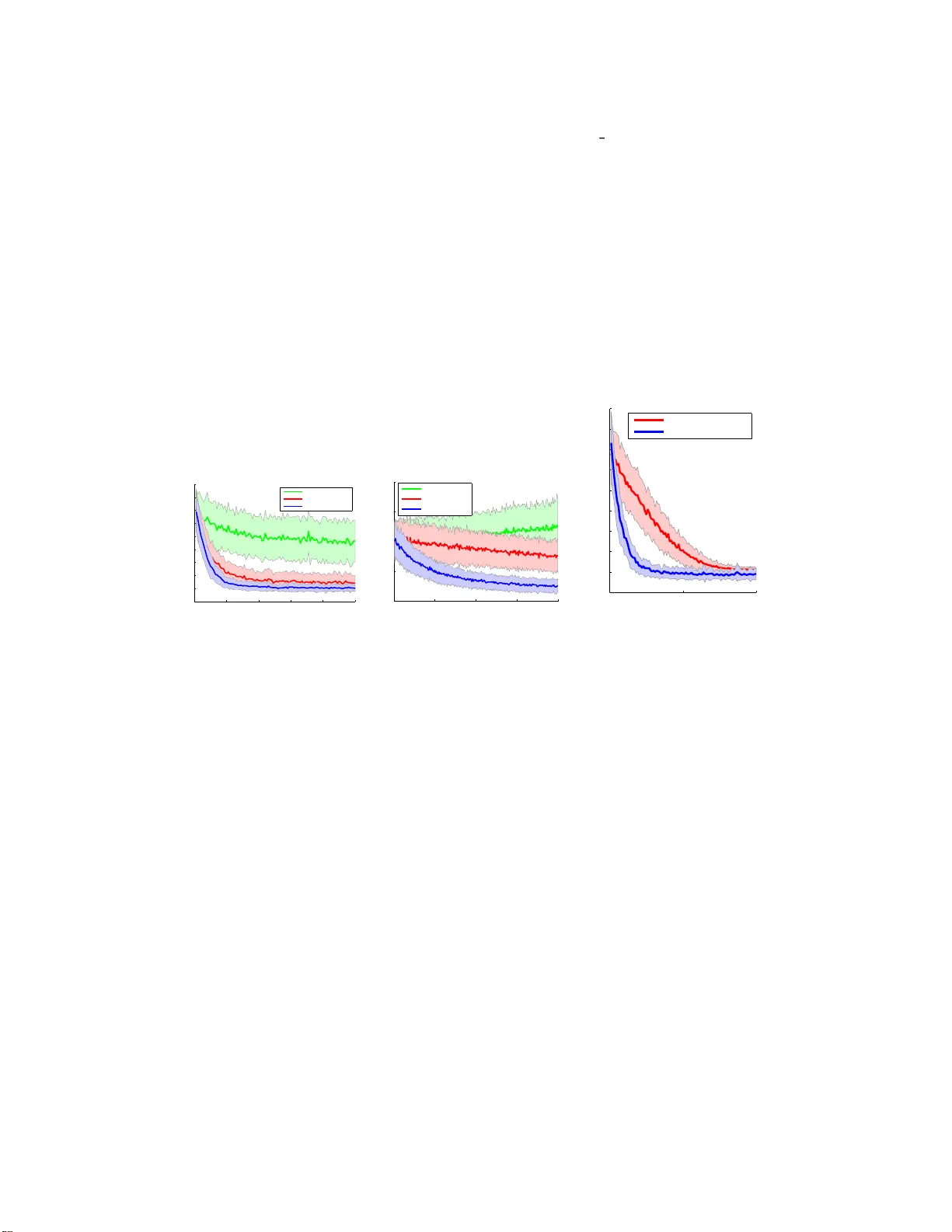
A utomated V ariational Inference in Probabilistic Pr ogramm in g David Wingate, Theo W eber Abstract W e pr esent a new algorithm fo r appro ximate inference in proba bilistic progr ams, based o n a stochastic g radient fo r variational pr ograms. Th is m ethod is ef ficient without restrictions on the prob abilistic pr ogram; it is particularly practical for distributions which are no t analytically tr actable, including h ighly structured dis- tributions that arise in pr obabilistic pro grams. W e sh ow how to auto matically derive mean-field probabilistic programs and op timize th em, and demo nstrate th at our perspective im proves inference ef ficiency ov er other algor ithms. 1 Intr oduction 1.1 A utomated V ariational I nference f or Pr obabilistic P rog r amming Probabilistic programming languages simplify the de velopment of pr obabilistic models by allo wing progr ammers to specify a stochastic proce ss using syntax that resembles modern progra mming lan- guages. These languages allo w progr ammers to freely mix deterministic and stochastic elements, resulting in tremendou s modeling fle xibility . The resultin g programs define prior distributions: run- ning the (uncond itional) prog ram forward many times results in a distribution over execution trace s, with each tr ace g enerating a sam ple o f d ata from the prior . T he goal of inf erence in such p rograms is to re ason about the posterior distribution over execution traces cond itioned on a particular pro gram output. Examples include BLOG [1], PRISM [2], B ay esian Logic Pro grams [3 ], Stochastic Logic Programs [4], Independ ent Cho ice Logic [5], IBAL [6], Prob abilistic Schem e [ 7], Λ ◦ [8], Church [9], Stochastic Matlab [10], and HANSEI [11]. It is easy to sample from the prior p ( x ) defined by a probabilistic program: simp ly run the program. But inf erence in such languages is hard : given a k nown value of a subset y of the variables, in ference must essentially run the program ‘backwards’ to sam ple from p ( x | y ) . Probabilistic programm ing en viro nments simplify inference by providing uni versal inf erence alg orithms; these are usually sam- ple based (MCMC or Gibbs) [1, 6, 9], due to their universality an d ease of implementation. V ariational inferen ce [1 2 – 14] offers a po werfu l, de terministic appr oximation to exact Bayesian in- ference in complex distrib ution s. The g oal is to approximate a co mplex distribution p by a simpler parametric distribution q θ ; inference therefore becom es the task of find ing the q θ closest to p , as mea- sured by KL divergence. If q θ is an easy distribution, this op timization can often be d one tractably; for example, the m ean-field approxim ation assumes that q θ is a p roduct of marginal distributions, which is easy to work with. Since variational inf erence techniqu es offer a comp elling alternative to sample b ased method s, it is o f interest to automatically derive them, especially for complex models. Un fortun ately , this is intractable fo r mo st pro grams. Even fo r mode ls which h av e closed-form coord inate d escent eq ua- tions, th e deriv ation s are often co mplex and cann ot be do ne by a compu ter . Howe ver, in this paper, we show that it is tractable to constru ct a stoch astic, gr adient-based variational inference algor ithm automatically by le veragin g compositiona lity . 1 2 A utomated V ariational Inference An uncond itional prob abilistic program f is defined as a parameterless function with an arbitra ry mix of deterministic and st oc hastic elements. Stoch astic elements can either belong to a fixed set of known, atomic r andom pro cedures called ERPs (for e le me ntary r an d om pr o c e dur es ), o r b e defin ed as function of other stochastic elements. The syntax and e valuation of a v alid program, as well as the definition o f the library of ERPs, define the prob abilistic programm ing lan guage. As the pr ogram f r uns, it will encou nter a sequence of ERPs x 1 , · · · , x T , a nd sample values for each. The set of sam pled values is called the trace o f the prog ram. Let x t be the value taken b y the t th ERP . The probab ility of a trace is giv en by the probab ility of each ERP taking the particular v alue ob served in the trace: p ( x ) = T Y t =1 p t ( x t | ψ t ( h t )) (1) where h t is the history ( x 1 , . . . , x t − 1 ) of the program up to ERP t , p t is the pro bability d istribution of the t th ERP , with h istory-dep endent par ameter ψ t ( h t ) . T r ace-based probabilistic pr ograms therefore define directed gr aphical mo dels, but in a more gen eral way than many classes of mo dels, since the language can allow comp lex program ming concepts such as flow control, recur sion, external libraries, data structures, etc. 2.1 KL Di vergence The goal of variational inferenc e [12 – 14] is to ap proxim ate the complex distribution p ( x | y ) with a simpler distrib ution p θ ( x ) . This is done by adjusting the parameters θ of p θ ( x ) in order to maximize a reward function L ( θ ) , typ ically giv en by the KL div ergence : K L ( p θ , p ( x | y )) = Z x p θ ( x ) log  p θ ( x ) p ( x | y )  = Z x p θ ( x ) log  p θ ( x ) p ( y | x ) p ( x )  + log p ( y ) = − L ( θ ) + log p ( y ) (2) where (3) L ( θ ) ∆ = Z x p θ ( x ) log  p ( y | x ) p ( x ) p θ ( x )  (4) Since the KL div ergen ce is nonnegative, the reward function L ( θ ) is a lower bound on the partition function log p ( y ) = log R x p ( y | x ) p ( x ) ; the approx imation error is therefore minimized by maximiz- ing the lower bound. Different cho ices o f p θ ( x ) result in different kind s o f app roximatio ns. The popu lar m ean-field ap- proxim ation decomposes p θ ( x ) into a prod uct o f m arginals as p θ ( x ) = Q T t =1 p θ ( x t | θ t ) , where every random choice ignores the history h t of the gene rativ e process. 2.2 Stochastic Gra dient Opt imiza tion Minimizing Eq . 2 is typically done b y com puting deriv atives analytica lly , setting them equal to zero, solving for a co upled set of no nlinear equatio ns, and d eriving an iter ati ve coo rdinate descent algorithm . Howe ver , th is approac h only works f or conjugate distributions, and fails f or highly struc- tured distributions (such as those rep resented b y , for example , proba bilistic p rogram s) that are n ot analytically tractable. 2 One gen eric appro ach to solv ing this is (stoch astic) gradient descen t on L ( θ ) . W e estimate the gradient accordin g to the following computation : −∇ θ L ( θ ) = Z x ∇ θ  p θ ( x ) log  p θ ( x ) p ( y | x ) p ( x )  (5) = Z x ∇ θ p θ ( x )  log  p θ ( x ) p ( y | x ) p ( x )  + Z x p θ ( x ) ( ∇ θ log( p θ ( x ))) (6) = Z x ∇ θ p θ ( x )  log  p θ ( x ) p ( y | x ) p ( x )  (7) = Z x p θ ( x ) ∇ θ log( p θ ( x ))  log  p θ ( x ) p ( y | x ) p ( x )  (8) = Z x p θ ( x ) ∇ θ log( p θ ( x ))  log  p θ ( x ) p ( y | x ) p ( x )  + K  (9) ≈ 1 N X x j ∇ θ log p θ ( x j )  log  p θ ( x j ) p ( y | x j ) p ( x j )  + K  (10) with x j ∼ p θ ( x ) , j = 1 . . . N and K is an arbitrary constant. T o o btain eq uations (7-9), we repeatedly use the fact tha t ∇ log p θ ( x ) = ∇ θ p θ ( x ) p θ ( x ) . Furtherm ore, for equations (7) and (9), we also use R x p θ ( x ) ∇ log p θ ( x ) = 0 , since R x p θ ( x ) ∇ log p θ ( x ) = R x ∇ θ p θ ( x ) = ∇ θ R x p θ ( x ) = ∇ θ 1 = 0 . The purp ose of add ing the constant K is tha t it is possible to appr oximately estimate a value of K (op timal b aseline), such th at the variance o f the Mon te-Carlo estimate (1 0) o f expression (9) is m inimized. As we will see, choosing a n app ropriate value of K will have drastic ef fects o n th e quality of the gradien t estimate. 2.3 Compositional V ariationa l Inference Consider a distribution p ( x ) in duced by an arbitrary , unconditional probab ilistic program. Ou r goal is to estimate marginals of the condition al distrib utio n p ( x | y ) , which we will call the targ et pr o - gram . W e intr oduce a variational distribution p θ ( x ) , wh ich is defined thro ugh anoth er probab ilistic progr am, ca lled the variational pr ogram . This distribution is unconditiona l, so sampling from it is as easy as runnin g it. W e derive the variational program from the target progr am. An easy way to do this is to use a partial me a n-field ap p r oximation : the target probabilistic pr ogram is run fo rward, and each time an ERP x t is encounter ed, a v ariational parameter is used in p lace of whate ver parameters w ould ordinar ily be passed to the ERP . That is, instead of s amp ling x t from p t ( x t | ψ t ( h t )) as in Eq. 1, we instead sample from p t ( x t | θ t ( h t )) , where θ t ( h t ) is an auxiliar y v ariationa l parameter (and the true parameter ψ t ( h t ) is igno red). Fig. 1 illustrates this w ith pseudo code f or a pro babilistic p rogram and its variational equiv alent: u pon encoun tering the normal ERP on line 4 , instead of using p arameter m u , the variational parameter θ 3 is used instead ( normal is a Gaussian ERP which takes an optional argument for th e mean, and rand(a,b) is uniform over the set [ a, b ] , with [0 , 1] as the default argument) . Note that a depend ency b etween X and M exists through the contro l logic, but not the parameterization. Thu s, in general, stochastic dep endencies due to the param eters of a variable depending on the o utcome of ano ther variable disappear, b ut d ependen cies due to contro l logic remain ( hence the term partial mean-fie ld a ppr oximation ) . This idea can be extend ed to auto matically compute th e stochastic gradient o f the v ariatio nal dis- tribution: we run the forward target prog ram no rmally , and whe nev er a call to an ERP x t is made, we: • Sample x t accordin g to p θ t ( x t ) (if this is t he first time the ERP is encounter ed, initialize θ t to an arbitrary value, for instance that given by ψ t ( h t ) ). • Comp ute the log-likelihood log p θ t ( x t ) o f x t accordin g to the mean-field distribution. • Comp ute the log-likelihood log p ( x t | h t ) o f x t accordin g to the target program. • Comp ute the re ward R t = log p ( x t | h t ) − lo g p θ ( x t ) 3 Probabilistic program A 1: M = normal(); 2: if M > 1 3: mu = complex deterministi c func( M ); 4: X = normal( mu ); 5: else 6: X = rand(); 7: end; Mean-Field varia tional program A 1: M = normal( θ 1 ); 2: if M > 1 3: mu = complex deterministi c func( M ); 4: X = normal( θ 3 ); 5: else 6: X = rand( θ 4 , θ 5 ); 7: end; Figure 1: A probabilistic program and correspondin g variational progr am • Comp ute the local gradient ψ t = ∇ θ t log p θ t ( x t ) . When the pro gram terminates, we simply comp ute log p ( y | x ) , then com pute the gain R = P R t + log p ( y | x ) + K . The g radient estimate for the t th ERP is gi ven b y Rψ t , and can be averaged over many sample traces x fo r a more accurate est imate. Thus, the only r equiremen t on the proba bilistic progr am is to be a ble to compu te the log likelihood of a n ERP value, as well as its gradient with re spect to its parame ters. Let us hig hlight that being able to compute the gradient of the log -likelihood with re spect to natural pa rameters is the only additional requirem ent compared to an MCMC sampler . Note that everything above holds: 1) re gar dless of con jugacy of distributions in the stochastic p ro- gram; 2) regardless of the contr ol logic of the stochastic program; and 3) regardless of the actual parametriza tion of p ( x t ; θ t ) . In par ticular , we again emph asize that we do no t need the grad ients of deterministic structures (for example, the function complex deterministi c func i n Fig. 1). 2.4 Extensions Here, we discuss three extensions of our core ideas. Learning inference transfer . Assume we wish to run variational inference for N distinct datasets y 1 , . . . , y N . Ideally , on e should solve a distinct inference pr oblem for each, yieldin g distinct θ 1 , · · · , θ N . Unf ortunately , finding θ 1 , · · · , θ N does not help to find θ N +1 for a n ew dataset y N +1 . But perhaps our approac h can be used to learn ‘approx imate sampler s’: instead of θ depending on y implicitly via th e op timization algorith m, suppo se instead that θ t depend s on y through some fixed function al form. For instance, we can as sum e θ t ( y ) = P j α i,j f j ( y ) , where f j is a known f unction, then find par ameters θ t,j such that for mo st observations y , th e variational distrib ution p θ ( y ) ( x ) is a decent approxim ate samp ler to p ( x | y ) . Gradient estimates of α can be derived similarly to Eq. 2 for arbitrary prob abilistic programs. Structured mean-field approximations. It is sometim es the case that a vanilla mean-field distribu- tion is a po or appr oximation of the po sterior, in which case more structured app roximatio ns should be u sed [15 – 18]. Deri vin g the variational u pdate for structu red mean -field is harder than vanilla mean-field; howev er, fro m a probab ilistic prog ram poin t of vie w , a structu red mean -field ap proxi- mation is simply a more complex (b ut still unco nditional) v ariational progr am that could be deri ved via progra m analysis (or perhaps online via RL state-space estimation), with gradients computed as in the mean-field case. Online probabilistic programming One advantage of stochastic gr adients in p robabilistic pro- grams is simple par allelizability . This can also be done in an onlin e fashion, in a similar fashion 4 to recent w or k for stoch astic v ariation al inf erence by Blei et al. [19 – 21]. Suppo se th at the set of variables and observ ation s can be separated into a main set X , and a large num ber N o f in depend ent sets of latent variables X i and observ ation s Y i (where the ( X i , Y i ) are on ly allo wed to dep end o n X ). For instance, for L D A, X rep resents the topic distributions, while th e X i represent th e docu- ment distribution over topics and Y i topic i . Recall the gradien t f or the variational parameters of X is g i ven by K ψ X , with K = R X + P i ( R i + lo g P ( Y i | X i , X ) , where R X is the sum of re- wards for all ERPs in X , an d R i is the sum o f rewards for all ERPs in X i . K can be rewritten as X + N E [ R v + log P ( Y v | X v , X ) , where v is a ran dom integer in { 1 , . . . , N } . The expectation can be ap proxim ately computed in an o nline fashion, allowing the upda te of the estimate of X without manipulatin g the entire data set Y . 3 Experiments: LD A and QMR 0 20 40 60 80 100 0 50 100 150 200 250 300 350 400 450 Iterations Divergence QMR Second−order GD Vanilla GD ENAC (a) Results on QMR 0 50 100 150 200 50 55 60 65 70 Iterations Divergence LDA Second−order GD Vanilla GD ENAC (b) Results on LDA 0 50 100 0 50 100 150 200 250 300 350 400 450 Iterations Divergence QMR Steepest Descent Conjugate Gradients (c) Steepest descent vs. con jugate gradients Figure 2: Nu merical simulations of A VI W e tested automated variational inf erence on two commo n inference b enchmar ks: the QMR-DT network (a b inary bipar tite graphical model with noisy-o r directed links) an d LDA (a popular topic model). W e comp ared three algorithms: • The first is vanilla stochastic gradient descent on Eq. 2, with the gradients giv en by Eq. 5. • The Episodic Natural Actor Critic algorithm, a version of th e algo rithm con necting variational inference to r einforcem ent learning – details are reserved for a longer version of this paper . An importan t feature of EN AC is o ptimizing over the baseline constant K . • A second- order gradient descent (SOGD) algorithm which estimates the Fisher information ma- trix F θ in the same way as the EN A C algorith m, and uses it as curvature information . For each a lgorithm, we set M = 10 (i.e., far fewer roll-ou ts than parameters) . All three algorithm s were gi ven th e same “budget” of samples; they used them in dif fer ent ways. All three alg orithms estimated a g radient ˆ g ( θ ) ; these were used in a steep est descent o ptimizer: θ = θ + α ˆ g ( θ ) with stepsize α . All three algor ithms used the s ame s tepsize; in ad dition, the grad ients g were scaled to have unit no rm. The e xper iment thu s d irectly comp ares th e quality of the direction of the g radient estimate. Fig. 3 s hows the r esults. The EN A C algorithm sho ws faster c on vergence a nd lo wer variance than steepest descent, while SOGD fares po orly (and even diverges in the case o f LD A). Fig. 3 also shows that the gradients fr om ENA C can be used either with steepest descent or a conjugate gradien t optimizer; conjuga te gradients con verge faster . Because both SOGD and ENA C estimate F θ in the same way , we conclude that the perfor mance advantage of ENA C is no t due solely to its use o f secon d-ord er infor mation: the addition al step o f estimating the baseline improves performa nce significantly . 5 Once conv erged, the estimated v ariatio nal program allo ws very f ast ap proxima te samp ling from the posterior, at a fraction o f the cost of a samp le obtained using MCMC samp ling. Samples f rom the variational program can als o be used as warm starts for MCMC sampling . 4 Related W ork Natural co njugate gradien ts for variational inference ar e inv estigated in [25], but the analysis is mostly de voted to the case where the variational approxim ation is Gaussian, and the resulting gradi- ent equation in volves an integral which is not necessarily tractable. The use o f variational inferen ce in prob abilistic prog ramming is explored in [29]. The autho rs similarly note th at it is easy to sample from the variational p rogram . Howe ver, they only use this observation to estimate the free energy of the variational progr am, but they do not estimate th e gradient of that fr ee energy . While they do hig hlight the need fo r o ptimizing th e parameter s of th e variational program, they do not offer a general algorithm for doing so, instead suggesting rejection sampling or importan ce sampling. Use of stochastic approxim ations fo r variational inferen ce is als o u sed by Carbonetto [30]. Their approa ch is very different from ou rs: th ey use Sequ ential Mon te Carlo to refine gradien t estimates, and require that the f amily of variational d istributions contain s the target distribution. While their approa ch is fairly general, it cannot be automatically generated for arbitrarily complex probab ilistic models. Finally , stochastic gradient methods are also used in onlin e v ariatio nal inference algorithms, in par- ticular in the work of Blei et al. in sto chastic variational infer ence (for instanc e, online LDA [19], o n- line HDP [20], and more generally un der conjugacy ass um ptions [21]), as a way to r efine estimates of latent v ariable d istributions without p rocessing all the ob servations. Howe ver, this appr oach re- quires a manual deriv ation of the v ariation al equation for coordinate descent, which is only possible under conjug acy assumptio ns which will in general not hold for arbitrary probabilistic programs. Refer ences [1] Brian Milch , Bhaskara Marthi, Stuart Russell, David So ntag, D aniel L. Ong , and And rey K olob ov . BLOG: Probabilistic models with unknown objects. In Internatio nal Joint Con- fer ence on Artificial Intelligence ( IJCAI) , pages 1352– 1359, 2005. [2] T . Sato an d Y . Kameya. PRISM: A symb olic-statistical modelin g lan guage. In International Joint Confer ence on Artificial Intelligence (IJCAI) , 1997. [3] K. K ersting and L. De R aedt. Bayesian logic programm ing: Theo ry and tool. In L. Getoor and B. T askar , editors, An Intr od uction to Statistical Relationa l Learning . MIT Press, 2007. [4] Stephen Muggleton. Stochastic logic p rogram s. I n New Generation Computing . Academic Press, 1996 . [5] David Poole. The independent choice logic and beyond. pages 222–2 43, 2008. [6] A vi Pfeffer . I B AL: A pro babilistic rational prog ramming lang uage. In Interna tional J oint Confer ence on Artificial Inte lligence (IJCAI) , pages 733–74 0. Morgan Kau fmann Publ., 2001. [7] Alexhey Radul. Report on the probab ilistic language scheme. T echnica l Report MIT - CSAIL- TR-2007 -059, Massachusetts Institute of T echnolog y , 200 7. [8] Sung woo Park, Frank Pfenning, and S eb astian Thrun. A probab ilistic language based on sam- pling functions. A CM T rans. Pr ogr am . Lang. Syst. , 31(1):1– 46, 2008. [9] Noah Goo dman, V ikash Mansing hka, Daniel Roy , Keith Bonawitz, and Joshu a T enen baum. Church: a lang uage for generative mod els. I n Uncertainty in Artificial Intelligence (U AI) , 2008. [10] David W ingate , Andreas Stuhlmu eller , and Noah D. Go odman . Lightwe ight implementatio ns of prob abilistic programmin g languages via transfor mational compilation. In Internationa l Confer ence on Artificial Intelligence and Statistics (AIST A TS) , 2011. [11] Oleg K iselyov and Chung-ch ieh Shan. Embedd ed probabilistic programm ing. In Domain- Specific La nguages , pages 360–3 84, 2009. 6 [12] M.J. Beal an d M. MA. V ariational algor ithms for approximate bayesian inference. Unpub- lished d octoral dissertation, Un iversity Colle ge London , 2003. [13] Mich ael I. Jordan, Zoubin Ghahraman i, an d T o mmi Jaakola. Introductio n to variational meth- ods for graphical models. Machine Learning , (37) :183–2 33, 199 9. [14] J. W inn and C.M. Bishop . V ariational message passing. J ourn al of Ma chine Learning Re- sear ch , 6(1):661, 2006. [15] A. Bou chard- C ˆ ot ´ e and M.I. Jord an. Optimization of structured mean field objectives. In Pr oceedings of the T wenty-F ifth Confer ence on Uncertainty in Artificial Intelligence , pages 67–74 . A UAI P ress, 2 009. [16] Z. Ghahraman i. On structured variational appr oximation s. University o f T o r onto T echnica l Report, CRG-TR- 97-1 , 1997. [17] C.M. Bisho p and J. W inn. Structur ed v ariation al distributions in vibes. Pr ocee d ings A rtificial Intelligence an d Statistics, K ey W est, Florida , 2003. [18] D. Geiger and C. Meek. Structured variational infer ence procedu res and their r ealizations. In Pr oc. AI Stats . Citeseer , 2005 . [19] M.D. Hoffman, D.M. Blei, and F . Bach. Online learning for latent dirichlet allocation. Ad- vances in Neural Informatio n Pr ocessing Sy stems , 23:856 –864, 2010. [20] C. W ang, J. P aisley , and D.M. Blei. Online variational inference for the hierarch ical dirichlet process. [21] D.M. Blei. Stochastic variational inference. 20 11. [22] Ed ward He rbst. Gradien t and Hessian-based MCMC for DSGE models (job market paper), 2010. [23] M.J. W ainwrigh t and M.I. Jordan . Graph ical models, exp onential families, and variational inference . F ound ations and T r ends R  in Machine Learnin g , 1(1-2):1–30 5, 20 08. [24] Jan Peter s, Seth u V ijayakumar, and Stefan Schaal. Natural actor-critic. In Eur op ean Confer - ence on Machine Learning (ECML) , pages 280–291, 2005. [25] A. Honkela, M. T ornio , T . Raik o, and J. Karhunen. Na tural co njugate g radient in v ariatio nal inference . In Neural Informa tion Pr ocessing , pag es 305–314. S pr inger, 2008. [26] S. Amari. Natural grad ient w or ks ef ficien tly in learning. Neural Comp utation , (10), 1998. [27] Sham A. K akade. Natur al policy gradient. In Neural Information Pr ocessing Systems ( NIPS) , 2002. [28] M. W elling, Y .W . T eh, and B. Kappen. Hyb rid variational/gibb s collapsed inference in topic models. In Pr oceed ings of th e Confer ence on Un certainty in Artifical Intelligenc e (U AI) , pages 587–5 94. Citeseer , 2008. [29] G. Harik and N. Shazeer . V ariation al pro gram inference. Arxiv p r eprint arXiv:1006 .0991 , 2010. [30] P . Carbone tto, M. Kin g, and F . Hamze. A stoch astic approximation meth od for inf erence in probab ilistic graphical models. In NIPS , volume 22, pages 216–22 4. Citeseer , 2009. 7