Approximate Bayesian computation and Bayes linear analysis: Towards high-dimensional ABC

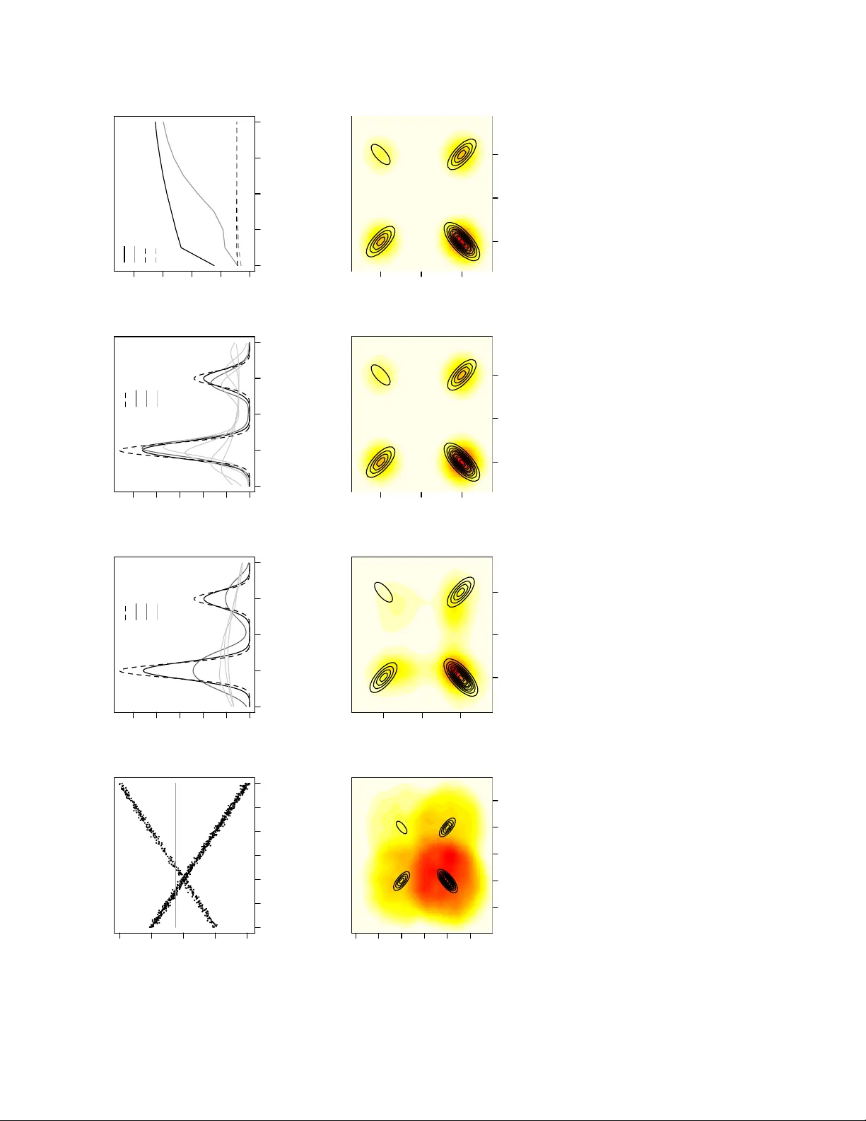
Appro ximate Ba y esian computation and Ba y es linear analysis: T o w ards high-dimensional ABC Da vid J. Nott ∗ , Y. F an † , L. Marshall ‡ and S. A. Sisson ‡ § No vem b er 27, 2024 Abstract Ba yes linear analysis and appro ximate Bay esian computation (ABC) are techniques commonly used in the Ba y esian analysis of complex mo dels. In this article w e con- nect these ideas by demonstrating that regression-adjustmen t ABC algorithms pro- duce samples for which first and second order momen t summaries approximate ad- justed exp ectation and v ariance for a Bay es linear analysis. This gives regression- adjustmen t metho ds a useful in terpretation and role in exploratory analysis in high- dimensional problems. As a result, we prop ose a new metho d for com bining high- dimensional, regression-adjustment ABC with lo w er-dimensional approaches (suc h as using MCMC for ABC). This metho d first obtains a rough estimate of the joint p os- terior via regression-adjustment ABC, and then estimates each univ ariate marginal p osterior distribution separately in a lo wer-dimensional analysis. The marginal dis- tributions of the initial estimate are then mo dified to equal the separately estimated marginals, thereby pro viding an improv ed estimate of the join t p osterior. W e illus- trate this method with sev eral examples. Supplementary materials for this article are a v ailable online. ∗ Departmen t of Statistics and Applied Probability , National Univ ersit y of Singap ore, Singap ore 117546. † Sc ho ol of Mathematics and Statistics, Univ ersity of New South W ales, Sydney 2052 Australia. ‡ Departmen t of Land Resources and Environmen tal Sciences, Montana State Universit y , 334 Leon John- son Hall, PO Box 173120, Bozeman, MT 59717-3120 § Comm unicating Author: Email Scott.Sisson@unsw.edu.au 1 Keyw ords : Approximate Bay esian computation; Bay es linear analysis; Computer mo dels; Densit y estimation; Likelihoo d-free inference; Regression adjustmen t. 1 In tro duction Ba yes linear analysis and appro ximate Bay esian computation (ABC) are tw o to ols that ha ve b een widely used for the appro ximate Ba y esian analysis of complex mo dels. Ba yes linear analysis can b e thought of either as an appro ximation to a con ven tional Ba yesian analysis using linear estimators of parameters, or as a fundamen tal extension of the sub jective Ba yesian approac h, where exp ectation rather than probability is a primitive quan tity and only elicitation of first and second order moments of v ariables of in terest is required (see e.g. Goldstein and W o off 2007 for an in tro duction). In this article, w e are interested in Ba yes linear metho ds to approximate a conv entional Bay esian analysis based on a probability mo del, and in particular in the setting where the likelihoo d is difficult to calculate. W e write p ( θ ) for the prior on a parameter θ = ( θ 1 , ..., θ p ) > , p ( y | θ ) for the likelihoo d and p ( θ | y ) for the p osterior. W e discuss Ba yes linear estimation further in the next section. Appro ximate Bay esian computation refers to a collection of metho ds which aim to draw samples from an approximate p osterior distribution when the lik eliho od, p ( y | θ ), is unav ail- able or computationally in tractable, but where it is feasible to quic kly generate data from the mo del y ∗ ∼ p ( y | θ ) (e.g. Lop es and Beaumont 2009; Bertorelle et al. 2010; Beaumon t 2010; Csill ´ ery et al. 2010; Sisson and F an 2011). The true p osterior is approximated b y p ( θ | y ) ≈ p ( θ | s ) where s = s ( y ) = ( s 1 , . . . , s d ) > is a lo w-dimensional vector of summary statistics (e.g. Blum et al. 2012). W riting p ( θ , s ∗ | s ) ∝ K  ( k s − s ∗ k ) p ( s ∗ | θ ) p ( θ ) , (1) where K  ( k u k ) = K ( k u k / ) / is a standard smo othing k ernel with scale parameter  > 0, 2 the appro ximate p osterior itself is constructed as p ( θ | s ) ≈ R p ( θ , s ∗ | s ) ds ∗ , following standard k ernel density estimation arguments. The form of (1) allo ws sampler-based ABC algorithms (e.g. Marjoram et al. 2003; Bortot et al. 2007; Sisson et al. 2007; T oni et al. 2009; Beaumon t et al. 2009; Dro v andi and Pettitt 2011) to sample from p ( θ , s ∗ | s ) without direct ev aluation of the likelihoo d. Regression has been prop osed as a w ay to impro v e up on the conditional densit y estimation of p ( θ | s ) within the ABC framework. Based on a sample ( θ 1 , y 1 ) , . . . , ( θ n , y n ) from p ( y | θ ) p ( θ ), and then transforming this to a sample ( θ 1 , s 1 ) , . . . , ( θ n , s n ) from p ( s | θ ) p ( θ ) through s i = s ( y i ), Beaumon t et al. (2002) considered the weigh ted linear regression mo del θ i = α + β > ( s i − s ) + ε i for i = 1 , . . . , n, (2) where ε i are indep enden t identically distributed errors, β is a d × p matrix of regression co efficien ts and α is a p × 1 vector. The weigh t for the pair ( θ i , s i ) is giv en by K  ( k s i − s k ). This regression mo del giv es a conditional density estimate of p ( θ | s i ) for an y s i . F or the observ ed s , this density estimate is an estimate of the p osterior of interest, p ( θ | s ), and α + ε i is a sample from it. W riting least squares estimates of α and β as ˆ α and ˆ β , and the resulting empirical residuals as ˆ ε i , then the regression-adjusted v ector θ i,a = θ i − ˆ β > ( s i − s ) ≈ ˆ α + ˆ ε i (3) is appro ximately a draw from p ( θ | s ). Beaumont et al. (2002) do not consider the mo del (2) as holding globally , but instead consider a local-linear fit (this is expressed through sp ecifying a k ernel, K  , with finite supp ort). V ariations on this idea include extensions to generalised linear mo dels (Leuenberger and W egmann 2010) and non-linear, heteroscedastic regression based on a feed-forw ard neural net w ork (Blum and F ran¸ cois 2010). The relativ e p erformance of the different regression adjustments are considered from a non-parametric p ersp ectiv e b y 3 Blum (2010). How ev er, application of regression-adjustment metho ds can fail in practice if the adopted regression model is clearly wrong, such as adopting the linear mo del (2) for a mixture, or mixture of regressions mo del. The qualit y of the appro ximation p ( θ | y ) ≈ p ( θ | s ) dep ends crucially on the form of the summary statistics, s . Equalit y p ( θ | y ) = p ( θ | s ) only o ccurs if s is sufficient for θ . How ev er, reliably obtaining sufficient statistics for complex mo dels is challenging (Blum et al. 2012), and so an ob vious strategy is to increase the dimension of the summary vector, d = dim( s ), to include as m uch information ab out y as p ossible. How ev er, the quality of the second appro ximation, p ( θ | s ) ≈ R p ( θ , s ∗ | s ) ds ∗ , is largely dep enden t on the matc hing of v ectors of summary statistics within the k ernel K  , whic h is itself dep enden t on the v alue of  . Through standard curse of dimensionality argumen ts (e.g. Blum 2010), for a given computational o verhead (e.g. for a fixed n um b er of samples ( θ i , s i )), the qualit y of the second appro ximation will deteriorate as d increases. As a result, given that more model parameters, θ , imply more summary statistics, s , this reality is a primary reason why ABC metho ds ha v e not, to date, found application in mo derate to high-dimensional analyses. In this article we mak e tw o primary contributions. First, w e sho w there is an interesting connection b et w een Ba y es linear analysis and regression-adjustmen t ABC metho ds. In par- ticular, samples from the regression-adjustmen t ABC algorithm of Beaumon t et al. (2002) result in first and second order moment summaries which directly approximate Bay es linear adjusted exp ectation and v ariance. This gives the linear regression-adjustmen t metho d a useful in terpretation for exploratory analysis in high dimensional problems. Motiv ated b y this connection, our second contribution is to prop ose a new metho d for com bining high-dimensional, regression-adjustment ABC with low er-dimensional ap- proac hes, such as MCMC. This metho d first obtains a rough estimate of the join t p osterior, p ( θ | s ), via regression-adjustment ABC, and then estimates each univ ariate marginal p oste- rior distribution, p ( θ i | s ), separately with a low er-dimensional ABC analysis. Estimation of 4 marginal distributions is substan tially easier than estimation of the joint distribution b e- cause of the lo w er dimensionalit y . The marginal distributions of the initial estimate are then mo dified to b e those of the estimated univ ariate marginals, thereby providing an impro ved estimate of the join t posterior. Similar ideas ha ve b een explored in the densit y estimation literature (e.g. Spiegelman and P ark 2003; Hall and Neumey er 2006; Giordani et al. 2009). As a result, w e are able to extend the applicabilit y of ABC methods to problems of moderate to high dimensionality – comfortably b ey ond current ABC practice. This article is structured as follows: Section 2 in tro duces Ba yes linear analysis, and explains its connection with the regression-adjustment ABC metho d of Beaumont et al. (2002). Section 3 describ es our prop osed marginal adjustment metho d for improving the estimate of the ABC joint p osterior distribution obtained using regression-adjustment ABC. A sim ulation study and real data analyses are presen ted in Section 4, and Section 5 concludes with a discussion. 2 A connection b et w een Ba y es linear analysis and ABC 2.1 Ba y es linear analysis As in Section 1, supp ose that s = s ( y ) = ( s 1 , ..., s d ) > is some vector of summary statistics based on data y , and that θ = ( θ 1 , ..., θ p ) > denotes parameter unknowns that w e wish to learn ab out. One view of Bay es linear analysis (e.g. Goldstein and W o off 2007) is that it aims to construct an optimal linear estimator of θ under squared error loss. That is, an estimator of the form a + B s , for a p -dimensional vector, a , and a p × d matrix, B , minimising E [( θ − a − B s ) > ( θ − a − B s )] . 5 The optimal linear estimator is giv en by E s ( θ ) = E ( θ ) + Cov( θ, s )V ar( s ) − 1 [ s − E ( s )] , (4) where exp ectations and cov ariances on the righ t hand side are with resp ect to the joint prior distribution of s and θ i.e. p ( s | θ ) p ( θ ). The estimator, E s ( θ ), is referred to as the adjusted exp ectation of θ given s . If the p osterior mean is a linear function of s then the adjusted exp ectation and p osterior mean coincide. Note that obtaining the b est linear estimator of θ do es not require sp ecification of a full prior or likelihoo d – only first and second order momen ts of ( θ, s ) are needed. F rom a sub jectiv e Ba yesian persp ectiv e, the need to make only a limited n umber of judgemen ts concerning prior momen ts is a k ey adv an tage of the Bay es linear approach. There are v arious interpretations of Ba y es linear metho ds – see Goldstein and W o off (2007), for further discussion. In the ABC context, a full probability mo del is typically av ailable. As such, w e will consider Bay es linear analysis from a con ven tional Ba yesian p oin t of view as a computational approximation to a full Bay esian analysis. The adjusted v ariance of θ given s , V ar s ( θ ) = E [( θ − E s ( θ )) > ( θ − E s ( θ )], can be shown to b e V ar s ( θ ) = V ar( θ ) − Cov( θ, s )V ar( s ) − 1 Co v( s, θ ) . F urthermore, the inequality V ar s ( θ ) ≥ E [V ar( θ | s )] holds, where A ≥ C means that A − C is non-negativ e definite, and the outer exp ectation on the right hand side is with resp ect to the prior distribution for s , p ( s ). This inequality indicates that V ar s ( θ ) is a generally conserv ativ e upp er b ound on p osterior v ariance, although it should b e noted that V ar s ( θ ) do es not depend on s , whereas V ar( θ | s ) is fully conditional on the observed s . If the p osterior mean is a linear function of s , then V ar s ( θ ) = E [V ar( θ | s )] 6 2.2 Ba y es linear analysis and regression adjustmen t ABC It is relativ ely straigh tforward to link the regression-adjustmen t approac h of Beaumon t et al. (2002) with a Bay es linear analysis. How ev er, note that Beaumon t et al. (2002) do not consider the mo del (2) as holding globally , but instead assume that it holds lo cally around the observed summary statistics, s . W e discuss this p oin t further b elo w, but for the moment w e assume that the unw eigh ted linear mo del (2) holds globally , after an appropriate c hoice of the summary statistics, s . The ordinary least squares estimate of β under the linear mo del (2) is ˆ β = ˆ Σ( s ) − 1 ˆ Σ( s, θ ), where ˆ Σ( s ) is the sample cov ariance of s 1 , ..., s n and ˆ Σ( s, θ ) is the sample cross cov ariance of the pairs ( s i , θ i ), i = 1 , ..., n . F or large n (where n is a quantit y under direct user control in an ABC analysis), ˆ β is approximately β = V ar( s ) − 1 Co v( s, θ ), where V ar( s ) and Co v( s, θ ) are the corresp onding p opulation versions of ˆ Σ( s ) and ˆ Σ( s, θ ). Let i b e fixed and consider the sequence of random v ariables θ i,a = θ i − ˆ β > ( s i − s ) as n tends to infinit y . Note that ˆ β is a function of ( θ j , s j ) for j = 1 , ..., n here. By Slutsky’s theorem, if ˆ β is consistent for β then θ i,a will conv erge in probability and in distribution to θ i − β > ( s i − s ) as n → ∞ . Then we can write lim n →∞ E ( θ i,a ) = E [ θ i − β > ( s i − s )] = E ( θ ) + Cov( θ, s )V ar( s ) − 1 [ s − E ( s )] = E s ( θ ) . where the in terchange of limits in the first line can b e justified b y applying the Sk oroho d represen tation theorem and then the dominated conv ergence theorem. 7 By a similar argument lim n →∞ V ar( θ i,a ) = V ar[ θ i − β > ( s i − s )] = V ar( θ ) + β > V ar( s ) β − 2Cov( θ, s ) β = V ar( θ ) − Cov( θ, s )V ar( s ) − 1 Co v( s, θ ) = V ar s ( θ ) . Hence, the co v ariance matrix of the regression-adjusted θ i,a appro ximates the Ba yes linear adjusted v ariance for large n . These results demonstrate that the first and second moments of the regression-adjusted samples θ i,a , i = 1 , ..., n in the linear metho d of Beaumont et al. (2002) hav e a useful in terpretation, regardless of whether the linear assumptions of the regression mo del (2) hold globally , as a Monte Carlo approximation to a Ba yes linear analysis. This connection with Ba yes linear analysis is not surprising when one considers that a Mon te Carlo approximation to (4) based on draws from the prior is just a least squares criterion for regression of θ on s . Usefully for our present purp oses, the Bay es linear in terpretation may b e helpful for motiv ating an exploratory use of regression adjustmen t ABC, even in problems of high dimension. In high-dimensional problems, an anon ymous referee has suggested it might also be useful to consider more sophisticated shrink age estimates of co v ariance matrices in implemen ting the Bay es linear approach. The connection b et ween Ba yes linear metho ds and regression-adjustmen t ABC con tinues to hold if kernel w eighting is reincorp orated into the regression model (2). Now consider the mo del (1) in general and a Ba yes linear analysis using first and second order momen ts of ( θ , s ∗ ) | s with Ba yes linear updating b y the information s = s ∗ . This then corresp onds to the kernel weigh ted version of the pro cedure of Beaumont et al. (2002). A recent extension of regression-adjustmen t ABC is the nonlinear, heteroscedastic metho d 8 of Blum and F ran¸ cois (2010) which replaces (2) with θ i = µ ( s i ) + σ ( s i ) ε i , (5) where µ ( s i ) = E ( θ | s = s i ) is a mean function, σ ( s i ) is a diagonal matrix with diagonal en tries equal to the square ro ots of the diagonal entries of V ar( θ | s = s i ), and the ε i are i.i.d. zero mean random vectors with V ar( ε i ) = I . It is p ossible also to tak e σ ( s ) to b e some matrix square ro ot of V ar( θ | s = s i ) where all elements are functions of s . If (5) holds, then the adjustmen t θ i,a = µ ( s ) + σ ( s ) σ ( s i ) − 1 [ θ i − µ ( s i )] is a dra w from p ( θ | s ). The heteroscedastic adjustment approac h do es seem to b e outside the Ba yes linear framew ork. Ho wev er, a nonlinear mean mo del for µ ( s ) with a constant mo del for σ ( s ) can b e reconciled with the Ba y es linear approach by considering an appropriate basis expansion inv olving functions of s . Blum (2010) gives some theoretical supp ort for more complex regression adjustmen ts through an analysis of a certain quadratic regression adjustmen t and suggests that transformations of θ can b e used to deal with heteroscedas- ticit y . In this case, the Bay es linear interpretation w ould b e more broadly applicable in regression-adjustmen t ABC. Another recent regression adjustment approac h is that of ? , whic h is based on fitting a flexible mixture mo del to the join t samples. An interesting recent related dev elopment is the semi-automatic metho d of choosing summary statistics of F ernhead and Prangle (2012). They consider an initial provisional set of statistics and then use linear regression to construct a summary statistic for eac h parameter, based on samples from the prior or some truncated version of it. Their approach can be seen as a use of Bay es linear estimates as summary statistics for an ABC analysis. There are several other innov ativ e asp ects of their pap er but their approach to summary statistic construction provides another strong link with Bay es linear ideas. 9 3 A marginal adjustmen t strategy Con ven tional sampler-based ABC metho ds, suc h as MCMC and SMC, which use rejection- or imp ortance w eight-based strategies, are hard to apply in problems of mo derate or high dimension. This o ccurs as an increase in the dimension of the parameter, θ , forces an increase in the dimension of the summary statistic, s . This, in turn, causes p erformance problems for sampler-based ABC metho ds as the term K  ( k s − s ∗ k ) in (1) suffers from the curse of dimensionalit y (Blum 2010). On the other hand, regression-adjustmen t strategies, which can often b e interpreted as Bay es linear adjustments (see Section 2), can b e useful in problems with man y parameters. How ev er, it is difficult to v alidate their accuracy , and sampler-based ABC metho ds may b e preferable in lo w dimensional problems, particularly when sim ulation under the mo del is computationally inexp ensiv e. W e now suggest a new approach to com bining the lo w-dimensional accuracy of sampler- based ABC metho ds, with the utility of the higher-dimensional, regression-adjustment ap- proac h. In essence, the idea is to construct a first rough estimate of the appro ximate p osterior using regression-adjustmen t ABC, and also separate estimates of each of the marginal distri- butions of θ 1 | s, . . . , θ p | s . Estimating marginal distributions is easier than the full p osterior, b ecause of the reduced dimensionalit y of summary statistics required to be informativ e about a single parameter. Because of the lo wer dimensionality , each marginal density can often b e more precisely estimated by an y sampler- or regression-based ABC metho d, than the same margin of the regression-based estimate of the join t distribution. W e then adjust the marginal distributions of the rough p osterior estimate to b e those of the separately estimated marginals, b y an appropriate replacemen t of order statistics. The adjustmen t of the marginal distributions main tains the multiv ariate dep endence structure in the original sample. When the marginals are w ell estimated, it is reasonable to exp ect that the join t p osterior is b etter estimated. 10 Precisely , the pro cedure w e use is as follows: 1. Generate a sample ( θ i , s i ), i = 1 , ..., n from p ( θ ) p ( s | θ ). 2. Obtain a regression adjusted sample θ i,a , i = 1 , ..., n based on either the mo del (2) or (5) fitted to the sample generated at Step 1. The regression adjusted metho ds ma y b e implemen ted with or without kernel w eighting. 3. F or j = 1 , ..., p , (a) F or the marginal mo del for θ j , p ( y | θ j ) = Z p ( y | θ ) p ( θ − j | θ j ) dθ − j , where θ − j is θ with the element θ j excluded, iden tify summary statistics s ( j ) = ( s ( j ) 1 , ..., s ( j ) d ( j ) ) > that are marginally informative for θ j . (b) Use a con ven tional ABC metho d to estimate the p osterior distribution for θ | s ( j ). Extracting the j th comp onen t results in a sample, θ m,i j , i = 1 , ..., n . If the num b er of samples drawn is not n , then we obtain a densit y estimate based on the samples w e hav e and then define θ m,i j , i = 1 , ..., n to b e n equally spaced quan tiles from the densit y estimate. (c) Replace the i = 1 , . . . , n order statistics for the j th comp onen t of the sample θ a,i , b y the equiv alen t quantiles of the marginal samples θ m,i j . More precisely , writing θ m, ( k ) j and θ a, ( k ) j as the k th order statistic of the samples θ m,i j and θ a,i j , resp ectiv ely , i = 1 , ..., n then we replace θ a, ( i ) j with θ m, ( i ) j for i = 1 , . . . , n . The samples, θ a,i , with all p margins adjusted are then tak en as an approximate sample from the ABC p osterior distribution. The samples used in Step 3 in the ab o v e algorithm can either b e the same as those generated in Step 1 or generated indep enden tly , but to 11 sa ve computational cost w e suggest using the same samples. An anonymous referee has suggested that it ma y b e p ossible to mak e use of the adjusted join t samples to help choose the summary statistics for the marginals, and this is an in triguing suggestion but something that w e lea v e to future w ork. The same referee has also p oin ted out the danger that the estimated marginals might not b e compatible with the dep endence structure in the join t distribution if there are parameter constraints - indeed, this can happ en for ordinary regression adjustment approac hes. Ho wev er, mostly suc h problems can b e dealt with through an appropriate reparameterisation. The idea of incorp orating knowledge of marginal distributions in to estimation of a joint distribution has b een previously explored in the density estimation literature. Spiegelman and P ark (2003) consider parametrically estimated marginal distributions and then replacing order statistics in the data b y the quantiles of the parametrically estimated marginals. This is similar in spirit to our adjustment pro cedure in the ABC context. They sho w by theoretical argumen ts and examples that impro vemen ts can b e obtained if the parametric assumptions are correct. Hall and Neumey er (2006) consider density estimation when there is a dataset of the joint distribution as well as additional datasets for the marginal distributions. They consider a copula approach to estimation of the joint density and sho w that the additional marginal information is b eneficial if the copula is sufficien tly smo oth. Recently , Giordani et al. (2009) hav e considered a mixture of normals copula approac h where the marginals are also estimated as mixtures of normals. A p o w erful motiv ation for using av ailable marginal information comes from the fact that a joint distribution is determined by the univ ariate distributions of all its linear pro jections. This arises as the characteristic function of the join t distribution is determined from the c haracteristic functions of one dimensional pro jections (Cram ´ er and W old 1936). Hence adjusting the distribution of all linear pro jections of a density estimate to b e correct would result in the true distribution b eing obtained. By adjusting marginal distributions we only 12 consider a selected small num b er of linear pro jections. How ev er, w e exp ect that if go od estimates of marginal distributions are av ailable, then transforming a rough estimate of the join t densit y to take these marginal distributions will b e b eneficial. Note that estimation and adjustment of the p marginal distributions in Step 3 ma y b e p erformed in parallel, so that computation scales w ell with the dimension of θ . Because the Bay es linear adjusted v ariance, V ar s ( θ ), is generally a conserv ativ e upp er b ound on the p osterior v ariance (see Section 2.1), it is credible that the initial rough samples θ i,a could form the basis of initial sampling distributions for imp ortance-t yp e ABC algorithms (e.g. Sisson et al. 2007; Beaumont et al. 2009; Drov andi and Pettitt 2011), resulting in p oten tial computational sa vings. Finally w e note that a n umber of metho ds exist to quic kly determine the appropriate statistics, s ( j ), for eac h marginal analysis. The reader is referred to Blum et al. (2012) for a comparative review of these. 4 Examples 4.1 A Sim ulated Example W e first construct a to y example where the likelihoo d can b e ev aluated and where a gold standard answer is av ailable for comparison. While ABC metho ds are not needed for the analysis of this mo del, it is instructive for understanding the prop erties of our metho ds. W e consider a p -dimensional Gaussian mixture mo del with 2 p mixture comp onen ts. The lik eliho o d for this mo del is given by p ( s | θ ) = 1 X b 1 =0 · · · 1 X b p =0 " p Y i =1 ω 1 − b i (1 − ω ) b i # φ p ( s | µ ( b, θ ) , Σ) , where φ p ( x | a, B ) denotes the p -dimensional Gaussian density function with mean a and co v ariance B ev aluated at x , ω ∈ [0 , 1] is a mixture weigh t, µ ( b, θ ) > = ((1 − 2 b 1 ) θ 1 , . . . , (1 − 13 2 b p ) θ p ), b = ( b 1 , . . . , b p ) with b i ∈ { 0 , 1 } and Σ = [Σ ij ] is such that Σ ii = 1 and Σ ij = ρ for i 6 = j . Under this setting, the marginal distribution for s i is given b y the tw o-comp onen t mixture p ( s i | θ i ) = (1 − ω ) φ 1 ( s i | − θ i , 1) + ω φ 1 ( s i | θ i , 1) . (6) The combination of the p tw o-mixture-comp onen t marginal distributions forms the 2 p mix- ture comp onen ts for the p -dimensional mo del. Giv en θ , data generation under this mo del pro ceeds b y indep enden tly generating each comp onen t of b to b e 0 or 1 with probabilities ω and 1 − ω resp ectiv ely , and then drawing s | θ , b ∼ φ p ( µ ( b, θ ) , Σ). F or the following analysis w e sp ecify s = (5 , 5 , . . . , 5), ω = 0 . 3 and ρ = 0 . 7, and re- strict the p osterior to ha ve finite supp ort on [ − 20 , 40] p , o v er whic h w e ha ve a uniform prior for θ . Computations are p erformed using 1 million simulations from p ( s | θ ) p ( θ ), using a uniform kernel K  ( k u k ), where k · k denotes Euclidean distance, and where  is c hosen to select the 10,000 simulations closest to s . W e con trast results obtained using standard rejec- tion sampling, rejection sampling follo w ed by the regression-adjustment of Beaumon t et al. (2002), and b oth of these after applying our marginal-adjustment strategy . All inferences w ere p erformed using the R pack age abc (Csill´ ery et al. 2011). Figure 1(a) illustrates the relationship b et w een θ 1 and s 1 (all margins are identical), with around 70% of summary statistics lo cated in the line with negativ e slop e. The observed summary statistic is indicated by the horizontal line, the marginal p osterior distribution for θ 1 defined by the implied densit y of summary statistics on this line. Figure 1(b) sho ws densit y estimates of θ 1 | s using rejection sampling for p = 1 , 2 , . . . , 5 mo del dimensions. The univ ariate true marginal distribution is indicated by the dashed line. As mo del dimension increases, the quality of the approximation to the true marginal distribution deteriorates rapidly . This is due to the curse of dimensionality in ABC (e.g. Blum 2010) in which the 14 -20 -10 0 10 20 30 40 -40 -20 0 20 40 θ 1 s 1 (a) -10 -5 0 5 10 0.00 0.10 0.20 θ 1 Density (b) True p=1 p=2 p=3,4,5 -10 -5 0 5 10 0.00 0.10 0.20 θ 1 Density (c) True p=1 p=2 p=4,6,8,10 2 4 6 8 10 0 1 2 3 4 Number of Dimensions KL Divergence (d) Rejection Linear Rejection (adj) Linear (adj) -10 -5 0 5 10 -10 -5 0 5 10 15 θ 1 θ 2 (e) -5 0 5 -5 0 5 θ 1 θ 2 (f) -5 0 5 -5 0 5 θ 1 θ 2 (g) -5 0 5 -5 0 5 θ 1 θ 2 (h) Figure 1: Inference on the Gaussian mixture mo del: Panel (a) plots the relationship b et ween θ 1 and s 1 . The horizontal line corresp onds to the observ ed summary statistic, s 1 = 5. Panels (b) and (c) sho w the estimated marginal p osterior for θ 1 resp ectiv ely using rejection sampling, and rejection sampling follow ed by regression-adjustmen t. Results are shown for a range of model dimensions, p . T rue marginal posterior is indicated b y the dashed line. P anel (d) sho ws the qualit y of the ABC appro ximation to the true mo del for the first tw o mo del parameters, ( θ 1 , θ 2 ), as measured by the Kullbac k-Leibler div ergence, as a function of mo del dimension, p . Black and grey lines resp ectiv ely denote rejection sampling and rejection sampling follo w ed by regression adjustmen t. Dashed lines indicate use of our marginal adjustment strategy . P anels (e)– (h) illustrate the ABC approximation to the biv ariate p osterior ( θ 1 , θ 2 ) | s when p = 3. Contours indicate the true mo del p osterior. Panels (e) and (f ) corresp ond resp ectiv ely to rejection sampling, and rejection sampling follow ed b y regression adjustmen t. P anels (g) and (h) corresp ond to panels (e) and (f ) with the addition of our marginal adjustment strategy . 15 restrictions on s 1 for a fixed n um b er of accepted samples (in this case 10,000) decrease within the comparison k s − s ∗ k as p increases. Of course one could increase the n umber of sim ulations as the dimension increases, but assuming a fixed computational budget returning a fixed n umber of samples provides one p ersp ectiv e on the curse of dimensionality here. Beyond p = 2 dimensions, these density estimates are exceptionally p o or. The same information is illustrated in Figure 1(c) after applying the linear regression-adjustment of Beaumont et al. (2002) to the samples obtained by rejection sampling in Figure 1(b). Clearly the regression- adjustmen t is b eneficial in providing impro ved marginal density estimates. Ho w ever, the qualit y of the appro ximation still deteriorates quic kly as p increases, alb eit more slowly than for rejection sampling alone. Figures 1(e) and (f ) sho w the tw o dimensional densit y estimates of ( θ 1 , θ 2 ) | s for the p = 3 dimensional mo del, resp ectiv ely using rejection sampling, and rejection sampling follow ed b y the linear regression-adjustment. The sup erimp osed contours corresp ond to those of the true biv ariate marginal distribution. The impro vemen t to the densit y estimate following the regression-adjustmen t is clear, how ever even here, the comp onen t mo des app ear to b e sligh tly misplaced, and there is some blurring of density with neigh b ouring comp onen ts. Figures 1(g) and (h) corresp ond to the densities in Figures 1(e) and (f ) after the im- plemen tation of our marginal adjustmen t strategy . Here, eac h margin of the distributions is adjusted to b e that of the appropriate univ ariate marginal density estimate in a p = 1 dimensional analysis. E.g. the margins for θ 1 are adjusted to b e exactly the ( p = 1) densit y estimates in Figures 1(b) and (c) . In b oth plots (g and h) there is a clear impro v ement in the biv ariate densit y estimate: the lo cations of the mixture components are in the correct places, and on the correct scales. Some of the accuracy of the dep endence structure is less well cap- tured under just rejection sampling, ho w ever (Figure 1(g)). Here, the correlation structure of eac h Gaussian comp onen t seems to b e p o orly estimated, compared to that obtained under the regression-adjustment transformed samples. The message here is clear: any marginal 16 adjustmen t strategy cannot reco ver from a p o orly estimated dep endence structure. The re- gression adjusted densit y in Figure 1(f ) more accurately captures the correlation structure of the true density , and this impro ved dep endence structure is carried o ver to the final densit y estimate in Figure 1(h). Finally , Figure 1(d) examines the quality of the ABC approximation to the true density , p ( θ | s ). Plotted is the Kullback-Leibler div ergence, R p ( θ ) log [ p ( θ ) /q ( θ )] dθ , b et w een the den- sities of the first t w o dimensions of eac h distribution as a function of model dimension (where p ( θ ) = p ( θ 1 , θ 2 | s ) is the true density , and q ( θ ) = q ( θ 1 , θ 2 | s ) is a k ernel density estimate of the ABC appro ximation). The div ergence is computed by Monte Carlo integration using 2,000 dra ws from the true density . W e compare only the first tw o dimensions of the p -dimensional p osteriors to main tain computational accuracy , noting that all pairwise marginal distribu- tions of the full p osterior are identical in this analysis (similarly for all higher-dimensional marginals) . Figure 1(d) largely supp orts our previous conclusions. The p erformance of the rejection sampler and the rejection sampler with regression-adjustment deteriorates rapidly as the n umber of mo del dimensions (i.e. summary statistics) increases, although the latter p erforms b etter in this regard. There is a clear improv ement to b oth of these approaches gained though our marginal adjustmen t strategy , with the mo dified regression-adjustmen t samples p erforming marginally b etter (for this example) where the original regression-adjustment pro vides b etter estimates of the multiv ariate dep endence structure in low er dimensions. After around p = 5 dimensions there is little difference b et w een the t wo marginally ad- justed p osteriors, and the divergence levels off to a constan t v alue indep enden t of mo del dimension. This is result of the ABC setup for this analysis. Beyond around p = 5 di- mensions, there is little difference b et ween the rejection sampling and regression-adjusted p osteriors (e.g. Figures 1(e) and (f )), b oth largely represen ting near-uniform distributions o ver θ . Hence, our marginal adjustment strategy is only able to make the same degree of 17 Figure 2: The heather incidence data representing a 10 × 20 metre region (Diggle, 1991). impro vemen ts, regardless of mo del dimension. The correlation dep endence structure is also lost beyond this point, so the expected b enefit of the regression-adjustmen t prior to marginal regression adjustmen t, is nullified. Using a low er initial threshold,  (computation p ermit- ting), w ould allo w a more accurate initial ABC analysis, and hence more discrimination b et w een the rejection sampling and regression-adjustmen t approac hes. 4.2 Excursion set mo del for heather incidence data W e now consider the medium resolution version of the heather incidence data analysed b y Diggle (1981), which is av ailable in the R pack age spatstat (Baddeley and T urner 2005). Figure 2 illustrates the data, consisting of a 256 × 512 grid of zeros and ones, with each binary v ariable representing presence (1) or absence (0) of heather at a particular spatial lo cation. Nott and Ryd ´ en (1999) used excursion sets of Gaussian random fields to mo del a lo w resolution version of these data. Without loss of generality , we assume that the data are observ ed on an integer lattice. Let { Y ( t ); t ∈ R 2 } b e a stationary Gaussian random field with mean zero and cov ariance 18 function R ( s, t ) = Cov( Y ( s ) , Y ( t )) = exp[ − ( t − s ) > A ( t − s )] where s, t ∈ R 2 and where A is a symmetric p ositiv e definite matrix. Hence R ( s, t ) cor- resp onds to the Gaussian cov ariance function mo del with elliptical anisotrop y . The u -level excursion set of Y ( t ) is defined as E u ( Y ) = { t ∈ R 2 : Y ( t ) ≥ u } , so that E u ( Y ) is obtained b y “thresholding” Y ( t ) at level u ∈ R . F or background on Gaussian random fields and geometric prop erties of their excursion sets see e.g. Adler and T a ylor (2007). W e mo del the heather data as binary random v ariables which are indicators for inclu- sion in an excursion set on an in teger lattice. The data are denoted B = { B ( i, j ) : i = 0 , ..., 255 , j = 0 , ..., 511 } where B ( i, j ) = I (( i, j ) ∈ E u ( Y )) and where I ( · ) denotes the in- dicator function. The distribution of B clearly dep ends on u and A . W e write the ( i, j )th elemen t of A as A ij . Since A is symmetric, A 12 = A 21 . W e parametrize the distribu- tion of B through θ = ( θ 1 , θ 2 , θ 3 , θ 4 ) where θ 1 = u , θ 2 = log A 11 , θ 3 = log A 22 and θ 4 = logit[( A 12 / √ A 11 A 22 + 1) / 2]. W e adopt the indep enden t prior distributions θ 1 ∼ N (0 , 0 . 5 2 ), θ 2 , θ 3 ∼ N ( − 4 , 0 . 5 2 ) and θ 4 ∼ N (0 , 0 . 5 2 ). The priors here are fairly noninformative. F or example, note that the exp ected fraction of ones in the image is 1 − Φ( θ 1 ). Hence if we were to use a normal prior for θ 1 with v ery large v ariance, this would give roughly prior probabil- it y 0.5 to having all zeros and probability 0.5 to hav e all ones. This is an unreasonable and highly informativ e prior. Our prior is fairly noninformative for the expected fraction of ones. Similarly our prior on θ 2 and θ 3 assigns roughly 95% prior probability for correlation in the east-w est and north-south directions at lag 10 resp ectiv ely b eing b et ween zero and 0.5. F or θ 4 , there is approximately 95% prior probability that A 12 / √ A 11 A 22 (a kind of correlation parameter describing the degree of anistropy for the cov ariance function) lies b et w een − 0 . 5 and 0 . 5. The results rep orted b elo w are not sensitiv e to c hanges in these priors within reason, 19 but as men tioned highly diffuse priors with large v ariances are not appropriate. Simulation of Gaussian random fields is achiev ed with the RandomFields pac k age in R (Sc hlather 2011), using the circulant em b edding algorithm of Dietrich and Newsam (1993) and W o o d and Chan (1994). F or summary statistics, denote b y n 11 ( v ) for v ∈ R 2 the num b er of pairs of v ariables in B , separated by displacemen t v , whic h are b oth 1. Similarly denote by n 00 ( v ) the n umber of suc h pairs whic h are b oth zero, and b y n 01 ( v ) the n umber of pairs where precisely one of the pair is 1 (the order do es not matter). In terms of estimating eac h marginal distribution θ 1 | s (1) , . . . , θ 4 | s (4), w e sp ecify s (1) = X i,j B ( i, j ) / (256 × 512) s (2) = [ n 11 ( v 1 ) , n 00 ( v 1 ) , n 01 ( v 1 )] > s (3) = [ n 11 ( v 2 ) , n 00 ( v 2 ) , n 01 ( v 2 )] > s (4) = [ n 11 ( v 3 ) , n 11 ( v 4 ) , n 00 ( v 3 ) , n 00 ( v 4 ) , n 01 ( v 3 ) , n 01 ( v 4 )] > as the summary statistics for each parameter, where v 1 = (0 , 1), v 2 = (1 , 0), v 3 = (1 , 1) and v 4 = (1 , − 1). F or the joint p osterior regression-adjustmen t, we used the heteroscedastic, non-linear regression (5) (Blum and F ran¸ cois 2010), using the uniform k ernel, K  ( k · k ), with scale parameter set to giv e non-zero weigh t to all 2 , 000 samples ( θ i , s i ) ∼ p ( s | θ ) p ( θ ), and where k · k represents scaled Euclidean distance. The individual marginal distributions were esti- mated in the same manner, but with the k ernel scale parameter sp ecified to select the 1,000 sim ulations closest to each s ( j ). All analyses were again p erformed using the R pac k age abc (Csill ´ ery et al. 2011) with the default settings for the heteroscedastic nonlinear metho d. Figure 3 shows estimated marginal p osterior distributions for the comp onen ts of θ ob- tained by the joint regression-adjustment (dotted lines), and the same margins follo wing 20 −0.15 −0.05 0.05 0.15 0 2 4 6 8 10 θ 1 Density −4.7 −4.6 −4.5 −4.4 0 2 4 6 8 θ 2 Density −4.8 −4.7 −4.6 −4.5 −4.4 0 2 4 6 8 θ 3 Density −0.3 −0.1 0.0 0.1 0.2 0.3 0 1 2 3 4 5 6 θ 4 Density Figure 3: Estimated marginal p osterior distributions of θ 1 , . . . , θ 4 for the heather incidence analysis. Solid lines denote individually estimated marginals; dotted lines illustrate estimated margins from the joint p osterior analysis 21 our marginal adjustmen t strategy (solid lines). The estimates for the spatial dep endence parameters θ 2 and θ 3 are p o or for the join t regression approach – the individually estimated marginals are estimated v ery accurately , whic h can be verified b y a rejection based analy- sis with a muc h larger num b er of samples (results not sho wn). Clearly if we use samples from the approximate join t p osterior distribution from the global regression for predictive inference or other purp oses, the fact that the unadjusted marginals are centred in the wrong place can lead to unacceptable p erformance of the approximation. It is interesting to understand why the global regression approac h fails here. Some insigh t can b e gained from Figure 4, which illustrates (prior predictiv e) scatter plots of θ 2 v ersus n 01 ( v 1 ) and θ 3 v ersus n 01 ( v 2 ). The summary statistics n 01 ( v 1 ) and n 01 ( v 2 ) are those whic h are most informativ e ab out θ 2 and θ 3 resp ectiv ely . If we consider regression of each of these parameters on the summary statistics, the graphs sho w that not only the mean and v ariance, but also higher order properties, such as sk ewness of the response, app ear to c hange as a function of the summary statistics. As such, the heteroscedastic regression-adjustmen t based on flexible estimation of the mean and v ariance do es not w ork well here. Making the regression lo cal for eac h marginal helps to ov ercome this problem. 4.3 Analysis of an A WBM computer mo del W e now examine metho ds for the analysis of computer mo dels, where we aim to accoun t for uncertain ty in high-dimensional forcing functions, assessmen t of mo del discrepancy and data rounding. An approximate treatmen t of this problem is interesting from a mo del assessmen t p oin t of view, where we w ant to judge whether the deficiencies of a computer mo del are such that the mo del ma y b e unfit for some purp ose. A computer mo del can b e regarded as a function y = f ( η ) where η are mo del inputs and y is a v ector of outputs. In mo delling some particular ph ysical system, observed data, d , is typically av ailable that corresp onds to some subset of the mo del outputs, y . The mo del 22 ● ● ● ● ● ● ● ● ● ● ● ● ● ● ● ● ● ● ● ● ● ● ● ● ● ● ● ● ● ● ● ● ● ● ● ● ● ● ● ● ● ● ● ● ● ● ● ● ● ● ● ● ● ● ● ● ● ● ● ● ● ● ● ● ● ● ● ● ● ● ● ● ● ● ● ● ● ● ● ● ● ● ● ● ● ● ● ● ● ● ● ● ● ● ● ● ● ● ● ● ● ● ● ● ● ● ● ● ● ● ● ● ● ● ● ● ● ● ● ● ● ● ● ● ● ● ● ● ● ● ● ● ● ● ● ● ● ● ● ● ● ● ● ● ● ● ● ● ● ● ● ● ● ● ● ● ● ● ● ● ● ● ● ● ● ● ● ● ● ● ● ● ● ● ● ● ● ● ● ● ● ● ● ● ● ● ● ● ● ● ● ● ● ● ● ● ● ● ● ● ● ● ● ● ● ● ● ● ● ● ● ● ● ● ● ● ● ● ● ● ● ● ● ● ● ● ● ● ● ● ● ● ● ● ● ● ● ● ● ● ● ● ● ● ● ● ● ● ● ● ● ● ● ● ● ● ● ● ● ● ● ● ● ● ● ● ● ● ● ● ● ● ● ● ● ● ● ● ● ● ● ● ● ● ● ● ● ● ● ● ● ● ● ● ● ● ● ● ● ● ● ● ● ● ● ● ● ● ● ● ● ● ● ● ● ● ● ● ● ● ● ● ● ● ● ● ● ● ● ● ● ● ● ● ● ● ● ● ● ● ● ● ● ● ● ● ● ● ● ● ● ● ● ● ● ● ● ● ● ● ● ● ● ● ● ● ● ● ● ● ● ● ● ● ● ● ● ● ● ● ● ● ● ● ● ● ● ● ● ● ● ● ● ● ● ● ● ● ● ● ● ● ● ● ● ● ● ● ● ● ● ● ● ● ● ● ● ● ● ● ● ● ● ● ● ● ● ● ● ● ● ● ● ● ● ● ● ● ● ● ● ● ● ● ● ● ● ● ● ● ● ● ● ● ● ● ● ● ● ● ● ● ● ● ● ● ● ● ● ● ● ● ● ● ● ● ● ● ● ● ● ● ● ● ● ● ● ● ● ● ● ● ● ● ● ● ● ● ● ● ● ● ● ● ● ● ● ● ● ● ● ● ● ● ● ● ● ● ● ● ● ● ● ● ● ● ● ● ● ● ● ● ● ● ● ● ● ● ● ● ● ● ● ● ● ● ● ● ● ● ● ● ● ● ● ● ● ● ● ● ● ● ● ● ● ● ● ● ● ● ● ● ● ● ● ● ● ● ● ● ● ● ● ● ● ● ● ● ● ● ● ● ● ● ● ● ● ● ● ● ● ● ● ● ● ● ● ● ● ● ● ● ● ● ● ● ● ● ● ● ● ● ● ● ● ● ● ● ● ● ● ● ● ● ● ● ● ● ● ● ● ● ● ● ● ● ● ● ● ● ● ● ● ● ● ● ● ● ● ● ● ● ● ● ● ● ● ● ● ● ● ● ● ● ● ● ● ● ● ● ● ● ● ● ● ● ● ● ● ● ● ● ● ● ● ● ● ● ● ● ● ● ● ● ● ● ● ● ● ● ● ● ● ● ● ● ● ● ● ● ● ● ● ● ● ● ● ● ● ● ● ● ● ● ● ● ● ● ● ● ● ● ● ● ● ● ● ● ● ● ● ● ● ● ● ● ● ● ● ● ● ● ● ● ● ● ● ● ● ● ● ● ● ● ● ● ● ● ● ● ● ● ● ● ● ● ● ● ● ● ● ● ● ● ● ● ● ● ● ● ● ● ● ● ● ● ● ● ● ● ● ● ● ● ● ● ● ● ● ● ● ● ● ● ● ● ● ● ● ● ● ● ● ● ● ● ● ● ● ● ● ● ● ● ● ● ● ● ● ● ● ● ● ● ● ● ● ● ● ● ● ● ● ● ● ● ● ● ● ● ● ● ● ● ● ● ● ● ● ● ● ● ● ● ● ● ● ● ● ● ● ● ● ● ● ● ● ● ● ● ● ● ● ● ● ● ● ● ● ● ● ● ● ● ● ● ● ● ● ● ● ● ● ● ● ● ● ● ● ● ● ● ● ● ● ● ● ● ● ● ● ● ● ● ● ● ● ● ● ● ● ● ● ● ● ● ● ● ● ● ● ● ● ● ● ● ● ● ● ● ● ● ● ● ● ● ● ● ● ● ● ● ● ● ● ● ● ● ● ● ● ● ● ● ● ● ● ● ● ● ● ● ● ● ● ● ● ● ● ● ● ● ● ● ● ● ● ● ● ● ● ● ● ● ● ● ● ● ● ● ● ● ● ● ● ● ● ● ● ● ● ● ● ● ● ● ● ● ● ● ● ● ● ● ● ● ● ● ● ● ● ● ● ● ● ● ● ● ● ● ● ● ● ● ● ● ● ● ● ● ● ● ● ● ● ● ● ● ● ● ● ● ● ● ● ● ● ● ● ● ● ● ● ● ● ● ● ● ● ● ● ● ● ● ● ● ● ● ● ● ● ● ● ● ● ● ● ● ● ● ● ● ● ● ● ● ● ● ● ● ● ● ● ● ● ● ● ● ● ● ● ● ● ● ● ● ● ● ● ● ● ● ● ● ● ● ● ● ● ● ● ● ● ● ● ● ● ● ● ● ● ● ● ● ● ● ● ● ● ● ● ● ● ● ● ● ● ● ● ● ● ● ● ● ● ● ● ● ● ● ● ● ● ● ● ● ● ● ● ● ● ● ● ● ● ● ● ● ● ● ● ● ● ● ● ● ● ● ● ● ● ● ● ● ● ● ● ● ● ● ● ● ● ● ● ● ● ● ● ● ● ● ● ● ● ● ● ● ● ● ● ● ● ● ● ● ● ● ● ● ● ● ● ● ● ● ● ● ● ● ● ● ● ● ● ● ● ● ● ● ● ● ● ● ● ● ● ● ● ● ● ● ● ● ● ● ● ● ● ● ● ● ● ● ● ● ● ● ● ● ● ● ● ● ● ● ● ● ● ● ● ● ● ● ● ● ● ● ● ● ● ● ● ● ● ● ● ● ● ● ● ● ● ● ● ● ● ● ● ● ● ● ● ● ● ● ● ● ● ● ● ● ● ● ● ● ● ● ● ● ● ● ● ● ● ● ● ● ● ● ● ● ● ● ● ● ● ● ● ● ● ● ● ● ● ● ● ● ● ● ● ● ● ● ● ● ● ● ● ● ● ● ● ● ● ● ● ● ● ● ● ● ● ● ● ● ● ● ● ● ● ● ● ● ● ● ● ● ● ● ● ● ● ● ● ● ● ● ● ● ● ● ● ● ● ● ● ● ● ● ● ● ● ● ● ● ● ● ● ● ● ● ● ● ● ● ● ● ● ● ● ● ● ● ● ● ● ● ● ● ● ● ● ● ● ● ● ● ● ● ● ● ● ● ● ● ● ● ● ● ● ● ● ● ● ● ● ● ● ● ● ● ● ● ● ● ● ● ● ● ● ● ● ● ● ● ● ● ● ● ● ● ● ● ● ● ● ● ● ● ● ● ● ● ● ● ● ● ● ● ● ● ● ● ● ● ● ● ● ● ● ● ● ● ● ● ● ● ● ● ● ● ● ● ● ● ● ● ● ● ● ● ● ● ● ● ● ● ● ● ● ● ● ● ● ● ● ● ● ● ● ● ● ● ● ● ● ● ● ● ● ● ● ● ● ● ● ● ● ● ● ● ● ● ● ● ● ● ● ● ● ● ● ● ● ● ● ● ● ● ● ● ● ● ● ● ● ● ● ● ● ● ● ● ● ● ● ● ● ● ● ● ● ● ● ● ● ● ● ● ● ● ● ● ● ● ● ● ● ● ● ● ● ● ● ● ● ● ● ● ● ● ● ● ● ● ● ● ● ● ● ● ● ● ● ● ● ● ● ● ● ● ● ● ● ● ● ● ● ● ● ● ● ● ● ● ● ● ● ● ● ● ● ● ● ● ● ● ● ● ● ● ● ● ● ● ● ● ● ● ● ● ● ● ● ● ● ● ● ● ● ● ● ● ● ● ● ● ● ● ● ● ● ● ● ● ● ● ● ● ● ● ● ● ● ● ● ● ● ● ● ● ● ● ● ● ● ● ● ● ● ● ● ● ● ● ● ● ● ● ● ● ● ● ● ● ● ● ● ● ● ● ● ● ● ● ● ● ● ● ● ● ● ● ● ● ● ● ● ● ● ● ● ● ● ● ● ● ● ● ● ● ● ● ● ● ● ● ● ● ● ● ● ● ● ● ● ● ● ● ● ● ● ● ● ● ● ● ● ● ● ● ● ● ● ● ● ● ● ● ● ● ● ● ● ● ● ● ● ● ● ● ● ● ● ● ● ● ● ● ● ● ● ● ● ● ● ● ● ● ● ● ● ● ● ● ● ● ● ● ● ● ● ● ● ● ● ● ● ● ● ● ● ● ● ● ● ● ● ● ● ● ● ● ● ● ● ● ● ● ● ● ● ● ● ● ● ● ● ● 5000 10000 15000 −5 −4 −3 −2 n 01 ( v 1 ) θ 2 ● ● ● ● ● ● ● ● ● ● ● ● ● ● ● ● ● ● ● ● ● ● ● ● ● ● ● ● ● ● ● ● ● ● ● ● ● ● ● ● ● ● ● ● ● ● ● ● ● ● ● ● ● ● ● ● ● ● ● ● ● ● ● ● ● ● ● ● ● ● ● ● ● ● ● ● ● ● ● ● ● ● ● ● ● ● ● ● ● ● ● ● ● ● ● ● ● ● ● ● ● ● ● ● ● ● ● ● ● ● ● ● ● ● ● ● ● ● ● ● ● ● ● ● ● ● ● ● ● ● ● ● ● ● ● ● ● ● ● ● ● ● ● ● ● ● ● ● ● ● ● ● ● ● ● ● ● ● ● ● ● ● ● ● ● ● ● ● ● ● ● ● ● ● ● ● ● ● ● ● ● ● ● ● ● ● ● ● ● ● ● ● ● ● ● ● ● ● ● ● ● ● ● ● ● ● ● ● ● ● ● ● ● ● ● ● ● ● ● ● ● ● ● ● ● ● ● ● ● ● ● ● ● ● ● ● ● ● ● ● ● ● ● ● ● ● ● ● ● ● ● ● ● ● ● ● ● ● ● ● ● ● ● ● ● ● ● ● ● ● ● ● ● ● ● ● ● ● ● ● ● ● ● ● ● ● ● ● ● ● ● ● ● ● ● ● ● ● ● ● ● ● ● ● ● ● ● ● ● ● ● ● ● ● ● ● ● ● ● ● ● ● ● ● ● ● ● ● ● ● ● ● ● ● ● ● ● ● ● ● ● ● ● ● ● ● ● ● ● ● ● ● ● ● ● ● ● ● ● ● ● ● ● ● ● ● ● ● ● ● ● ● ● ● ● ● ● ● ● ● ● ● ● ● ● ● ● ● ● ● ● ● ● ● ● ● ● ● ● ● ● ● ● ● ● ● ● ● ● ● ● ● ● ● ● ● ● ● ● ● ● ● ● ● ● ● ● ● ● ● ● ● ● ● ● ● ● ● ● ● ● ● ● ● ● ● ● ● ● ● ● ● ● ● ● ● ● ● ● ● ● ● ● ● ● ● ● ● ● ● ● ● ● ● ● ● ● ● ● ● ● ● ● ● ● ● ● ● ● ● ● ● ● ● ● ● ● ● ● ● ● ● ● ● ● ● ● ● ● ● ● ● ● ● ● ● ● ● ● ● ● ● ● ● ● ● ● ● ● ● ● ● ● ● ● ● ● ● ● ● ● ● ● ● ● ● ● ● ● ● ● ● ● ● ● ● ● ● ● ● ● ● ● ● ● ● ● ● ● ● ● ● ● ● ● ● ● ● ● ● ● ● ● ● ● ● ● ● ● ● ● ● ● ● ● ● ● ● ● ● ● ● ● ● ● ● ● ● ● ● ● ● ● ● ● ● ● ● ● ● ● ● ● ● ● ● ● ● ● ● ● ● ● ● ● ● ● ● ● ● ● ● ● ● ● ● ● ● ● ● ● ● ● ● ● ● ● ● ● ● ● ● ● ● ● ● ● ● ● ● ● ● ● ● ● ● ● ● ● ● ● ● ● ● ● ● ● ● ● ● ● ● ● ● ● ● ● ● ● ● ● ● ● ● ● ● ● ● ● ● ● ● ● ● ● ● ● ● ● ● ● ● ● ● ● ● ● ● ● ● ● ● ● ● ● ● ● ● ● ● ● ● ● ● ● ● ● ● ● ● ● ● ● ● ● ● ● ● ● ● ● ● ● ● ● ● ● ● ● ● ● ● ● ● ● ● ● ● ● ● ● ● ● ● ● ● ● ● ● ● ● ● ● ● ● ● ● ● ● ● ● ● ● ● ● ● ● ● ● ● ● ● ● ● ● ● ● ● ● ● ● ● ● ● ● ● ● ● ● ● ● ● ● ● ● ● ● ● ● ● ● ● ● ● ● ● ● ● ● ● ● ● ● ● ● ● ● ● ● ● ● ● ● ● ● ● ● ● ● ● ● ● ● ● ● ● ● ● ● ● ● ● ● ● ● ● ● ● ● ● ● ● ● ● ● ● ● ● ● ● ● ● ● ● ● ● ● ● ● ● ● ● ● ● ● ● ● ● ● ● ● ● ● ● ● ● ● ● ● ● ● ● ● ● ● ● ● ● ● ● ● ● ● ● ● ● ● ● ● ● ● ● ● ● ● ● ● ● ● ● ● ● ● ● ● ● ● ● ● ● ● ● ● ● ● ● ● ● ● ● ● ● ● ● ● ● ● ● ● ● ● ● ● ● ● ● ● ● ● ● ● ● ● ● ● ● ● ● ● ● ● ● ● ● ● ● ● ● ● ● ● ● ● ● ● ● ● ● ● ● ● ● ● ● ● ● ● ● ● ● ● ● ● ● ● ● ● ● ● ● ● ● ● ● ● ● ● ● ● ● ● ● ● ● ● ● ● ● ● ● ● ● ● ● ● ● ● ● ● ● ● ● ● ● ● ● ● ● ● ● ● ● ● ● ● ● ● ● ● ● ● ● ● ● ● ● ● ● ● ● ● ● ● ● ● ● ● ● ● ● ● ● ● ● ● ● ● ● ● ● ● ● ● ● ● ● ● ● ● ● ● ● ● ● ● ● ● ● ● ● ● ● ● ● ● ● ● ● ● ● ● ● ● ● ● ● ● ● ● ● ● ● ● ● ● ● ● ● ● ● ● ● ● ● ● ● ● ● ● ● ● ● ● ● ● ● ● ● ● ● ● ● ● ● ● ● ● ● ● ● ● ● ● ● ● ● ● ● ● ● ● ● ● ● ● ● ● ● ● ● ● ● ● ● ● ● ● ● ● ● ● ● ● ● ● ● ● ● ● ● ● ● ● ● ● ● ● ● ● ● ● ● ● ● ● ● ● ● ● ● ● ● ● ● ● ● ● ● ● ● ● ● ● ● ● ● ● ● ● ● ● ● ● ● ● ● ● ● ● ● ● ● ● ● ● ● ● ● ● ● ● ● ● ● ● ● ● ● ● ● ● ● ● ● ● ● ● ● ● ● ● ● ● ● ● ● ● ● ● ● ● ● ● ● ● ● ● ● ● ● ● ● ● ● ● ● ● ● ● ● ● ● ● ● ● ● ● ● ● ● ● ● ● ● ● ● ● ● ● ● ● ● ● ● ● ● ● ● ● ● ● ● ● ● ● ● ● ● ● ● ● ● ● ● ● ● ● ● ● ● ● ● ● ● ● ● ● ● ● ● ● ● ● ● ● ● ● ● ● ● ● ● ● ● ● ● ● ● ● ● ● ● ● ● ● ● ● ● ● ● ● ● ● ● ● ● ● ● ● ● ● ● ● ● ● ● ● ● ● ● ● ● ● ● ● ● ● ● ● ● ● ● ● ● ● ● ● ● ● ● ● ● ● ● ● ● ● ● ● ● ● ● ● ● ● ● ● ● ● ● ● ● ● ● ● ● ● ● ● ● ● ● ● ● ● ● ● ● ● ● ● ● ● ● ● ● ● ● ● ● ● ● ● ● ● ● ● ● ● ● ● ● ● ● ● ● ● ● ● ● ● ● ● ● ● ● ● ● ● ● ● ● ● ● ● ● ● ● ● ● ● ● ● ● ● ● ● ● ● ● ● ● ● ● ● ● ● ● ● ● ● ● ● ● ● ● ● ● ● ● ● ● ● ● ● ● ● ● ● ● ● ● ● ● ● ● ● ● ● ● ● ● ● ● ● ● ● ● ● ● ● ● ● ● ● ● ● ● ● ● ● ● ● ● ● ● ● ● ● ● ● ● ● ● ● ● ● ● ● ● ● ● ● ● ● ● ● ● ● ● ● ● ● ● ● ● ● ● ● ● ● ● ● ● ● ● ● ● ● ● ● ● ● ● ● ● ● ● ● ● ● ● ● ● ● ● ● ● ● ● ● ● ● ● ● ● ● ● ● ● ● ● ● ● ● ● ● ● ● ● ● ● ● ● ● ● ● ● ● ● ● ● ● ● ● ● ● ● ● ● ● ● ● ● ● ● ● ● ● ● ● ● ● ● ● ● ● ● ● ● ● ● ● ● ● ● ● ● ● ● ● ● ● ● ● ● ● ● ● ● ● ● ● ● ● ● ● ● ● ● ● ● ● ● ● ● ● ● ● ● ● ● ● ● ● ● ● ● ● ● ● ● ● ● ● ● ● ● ● ● ● ● ● ● ● ● ● ● ● ● ● ● ● ● ● ● ● ● ● ● ● ● ● ● ● ● ● ● ● ● ● ● ● ● ● ● ● ● ● ● ● ● ● ● ● ● ● ● ● ● ● ● ● ● ● ● ● ● ● ● ● ● ● ● ● ● ● ● ● ● ● ● ● ● ● ● ● ● ● ● ● ● ● ● ● ● ● ● ● ● ● ● ● ● ● ● ● ● ● ● ● ● ● ● ● ● ● ● ● ● ● ● ● ● ● ● ● ● ● ● ● ● ● ● ● ● ● ● ● ● ● ● ● ● ● ● ● ● ● ● ● ● ● ● ● ● ● ● ● ● ● ● ● ● ● ● ● ● ● ● 5000 10000 15000 −5.5 −5.0 −4.5 −4.0 −3.5 −3.0 −2.5 n 01 ( v 2 ) θ 3 Figure 4: Plot of θ 2 v ersus n 01 ( v 1 ) (left) and θ 3 v ersus n 01 ( v 2 ) (right) for samples from the prior for the heather incidence data. inputs, η , can b e of differen t t yp es. Here w e only mak e the distinction betw een model pa- rameters, θ ∗ , and forcing function inputs, ω , so that η = ( ω , θ ∗ ). Commonly , measurements of the forcing function inputs are av ailable, and uncertaint y in these inputs (due to e.g. sam- pling and measuremen t errors) will be ignored in an y analysis due to the high-dimensionalit y in volv ed. An uncertaint y analysis (inv olving an order of magnitude assessmen t of output uncertain ty due to forcing function uncertaint y) will often b e p erformed, rather than at- tempting to include forcing function uncertaint y directly in a calibration exercise (see, for example, Goldstein et al. 2010, for an example of this in the context of a h ydrological model). See e.g. Craig et al. (1997), Goldstein and Rougier (2009), Kennedy and O’Hagan (2001) and Goldstein et al. (2010) for further discussion of different asp ects of computer mo dels. W e no w assume that y = f ( η ) corresp onds to a prediction of the observed data d in the mo del d = f ( η ) + g + e, (7) 23 Precipitation ET c 1 c 2 c 3 a 1 a 2 a 3 Base Storage Baseflow Recharge = BFI×Excess Baseflow = (1-K)× Base Storage Surface runoff = ( 1-BFI ) ×Excess Figure 5: The three-catc hment Australian w ater balance mo del. where e denotes measuremen t error and other sources of error indep enden t in time, and g is a correlated error term represen ting external mo del discrepancy (see Goldstein et al. 2010 for a discussion of the differences b et w een internal and external mo del discrepancies). W e directly inv estigate forcing function uncertaint y , through the term f ( η ), using ABC. In the analysis of the mo del (7), we also consider data rounding effects, so that simulations pro duced from (7) are rounded according to the precision of the data that w as collected. Handling suc h rounding effects is v ery simple in the ABC framew ork. As a computer mo del, w e consider the Australian W ater Balance Mo del (A WBM) (Bough ton 2004), a rainfall-runoff mo del widely used in Australia for applications suc h as estimating catc hment water yield or designing floo d managemen t systems. As sho wn in Figure 5, the mo del consists of three surface stores, with depths c 1 , c 2 , c 3 and fractional areas a 1 , a 2 , a 3 with P k a k = 1, and a base store. Mo del forcing inputs are precipitation and ev apotran- spiration time series, from whic h a predicted streamflo w is produced. At each time step in the mo del, precipitation is added to the system and ev ap otranspiration subtracted, with the net input split b et w een the surface stores in prop ortion to the fractional areas. An y excess 24 ab o v e the surface store depths is then split b et ween surface runoff and flow into the base store according to the baseflo w index 0 < B F I < 1. W ater from the base store is disc harged in to the stream at a rate determined by the recession constant 0 < K < 1, and the total disc harge (streamflow) is then determined as the sum of the surface runoff and the baseflow. F ollo wing Bates and Campb ell (2001), we fix B F I = 0 . 4, although in some applications it may be b eneficial to allow this parameter to v ary . The mo del parameters are therefore θ ∗ = ( c 1 , c 2 , c 3 , a 1 , a 2 , K ), as well as the high-dimensional ev ap otranspiration and precipita- tion forcing inputs, ω . In h ydrological applications there is often great uncertain ty about the precipitation inputs in particular, due to measurement and sampling errors. Here we assume that ev apotranspiration is fixed (known), and w e use ω obs to denote the series of observ ed precipitation v alues only . In running the computer mo del, we initialize with all stores empty and discard the first 500 days of the sim ulation to discoun t the effect of the assumed initial conditions. Our data consist of a sequence of 5500 consecutiv e daily streamflo w v alues from a station at Blac k River at Bruce Highw ay in Queensland, Australia. The catc hmen t cov ers an area of 260km 2 with a mean annual rainfall of 1195mm. T o complete the determination of the computer mo del (7), we sp ecify the mo del priors. W riting η = ( ω , θ ∗ ), w e describ e the uncertaint y on the true forcing inputs, ω = ( ω 1 , . . . , ω T ), as ω t = δ t ω obs,t , where the random multiplicativ e terms hav e prior log δ t ∼ N ( − σ 2 δ / 2 , σ 2 δ ) for t = 1 , ..., T . W e set σ δ ∼ U (0 , 0 . 1), and note that E ( δ t ) = 1 a priori . F or the external mo del discrepancy parameters, g = ( g 1 , . . . , g T ) > , we sp ecify g ∼ N (0 , Σ g ) where Σ g = [Σ g ,ij ] is suc h that Σ g ,ij = σ 2 g exp( − ρ | i − j | ) , σ g ∼ U (0 , 0 . 1) and ρ ∼ U (0 . 1 , 1). Independent mo del errors, e = ( e 1 , . . . , e T ) > , are assumed to b e e t ∼ N (0 , σ 2 e ), for t = 1 , ..., T where σ e ∼ U [0 , 2]. A WBM parameter priors are sp ecified as c 1 ∼ U (0 , 500), c 2 − c 1 ∼ U (0 , 1000), c 3 − c 2 ∼ U (0 , 1000), [log( a 1 /a 3 ) , log( a 2 /a 3 )] > ∼ N (0 , 0 . 5 2 I ) and K ∼ 0 . 271 × Beta(5 . 19 , 4 . 17) + (1 − 0 . 271) × Beta(255 , 9 . 6), where the latter is a mixture of beta distributions. See Bates and Campb ell (2001) for discussion of the bac kground kno wledge leading to this prior c hoice. 25 If we treat the forcing inputs, ω , as nuisance parameters, our parameter of in terest is θ = ( θ ∗> , γ > ) > , the set of A WBM mo del parameters, and γ = ( σ e , σ g , σ q , ρ ) > , those param- eters sp ecifying distributions of the stochastic terms in (7). The ABC approach provides a con venien t wa y of integrating out the high-dimensional nuisance parameter, ω , while dealing with complications such as rounding in the recorded data (the streamflow data are rounded to the nearest 0.01mm). This w ould b e very challenging using conv en tional Ba yesian com- putational approac hes. T o define summary statistics, denote ˆ θ ∗ as the p osterior mo de estimate of θ ∗ in a mo del where w e assume no input uncertaint y , ω = ω obs , and where w e log-transform b oth the data and mo del output. Also denote b y s γ = [ ψ (0) , ψ (1) , ψ (2) , ζ (1) , ζ (2) , ζ (3)] > , where ψ ( j ) is the lag j auto co v ariance of the least squares residuals d − f ( ˆ η ), and ζ ( j ) is the lag j auto co v ariance of ( d − f ( ˆ η )) 2 with ˆ η = ( ω obs , ˆ θ ∗ ). In the notation of Section 3, for summary statistics for θ j , j = 1 , ..., 6 (i.e. the comp onen ts of θ ∗ ; the A WBM parameters) w e use the statistic s ( j ) = ˆ θ ∗ j and for θ j , j = 7 , ..., 10 (i.e. the comp onen ts of γ ) w e use the statistic s ( j ) = s γ . In effect, the summary statistics for θ ∗ consist of p oin t estimates for the A WBM parameters under the assumption of no error in the forcing inputs, ω , and statistics for the mo del error parameters, γ , are intuitiv ely based on auto co v ariances of residuals and squared residuals. Optimisation of ˆ θ ∗ is not trivial, as the ob jective function ma y hav e m ultiple mo des. T o pro vide some degree of robustness, we select the b est of ten Nelder-Mead simplex optimisations (Nelder and Mead 1965) using starting v alues simulated from the prior. Estimated marginal p osterior distributions for the parameters are shown in Figure 6. F or the join t-p osterior analysis, we implemented the non-linear, heteroscedastic, regression- adjustmen t of Blum and F ran¸ cois (2010) using the uniform k ernel, K  ( k · k ), with scale parameter set to giv e non-zero weigh t to all 2,000 samples ( θ i , s i ) ∼ p ( s | θ ) p ( θ ). F or the indi- vidually estimated margins, the scale parameter w as sp ecified to select the 500 simulations closet to each s ( j ). The discrepancy b et w een estimates for the parameters c 1 , K and σ e 26 0 100 200 300 400 500 0.000 0.015 c 1 0 500 1000 1500 0.0000 0.0015 c 2 500 1000 1500 2000 2e−04 1e−03 c 3 0.1 0.2 0.3 0.4 0.5 0.6 0 1 2 3 4 p 1 0.1 0.2 0.3 0.4 0.5 0.6 0.7 0.8 0.0 1.5 3.0 p 2 0.0 0.1 0.2 0.3 0.4 0.5 0.6 0 2 4 6 p 3 0.90 0.92 0.94 0.96 0.98 1.00 0 100 250 K 0.00 0.02 0.04 0.06 0.08 0.10 5 7 9 11 σ g 0.0 0.5 1.0 1.5 2.0 0.0 0.6 1.2 σ e 0.00 0.02 0.04 0.06 0.08 0.10 6 8 10 σ δ 0.2 0.4 0.6 0.8 1.0 0.6 0.9 1.2 ρ ● ● ● ● ● ● ● ● ● ● ● ● ● ● ● ● ● ● ● ● ● ● ● ● ● ● ● ● ● ● ● ● ● ● ● ● ● ● ● ● ● ● ● ● ● ● ● ● ● ● ● ● ● ● ● ● ● ● ● ● ● ● ● ● ● ● ● ● ● ● ● ● ● ● ● ● ● ● ● ● ● ● ● ● ● ● ● ● ● ● ● ● ● ● ● ● ● ● ● ● ● ● ● ● ● ● ● ● ● ● ● ● ● ● ● ● ● ● ● ● ● ● ● ● ● ● ● ● ● ● ● ● ● ● ● ● ● ● ● ● ● ● ● ● ● ● ● ● ● ● ● ● ● ● ● ● ● ● ● ● ● ● ● ● ● ● ● ● ● ● ● ● ● ● ● ● ● ● ● ● ● ● ● ● ● ● ● ● ● ● ● ● ● ● ● ● ● ● ● ● ● ● ● ● ● ● ● ● ● ● ● ● ● ● ● ● ● ● ● ● ● ● ● ● ● ● ● ● ● ● ● ● ● ● ● ● ● ● ● ● ● ● ● ● ● ● ● ● ● ● ● ● ● ● ● ● ● ● ● ● ● ● ● ● ● ● ● ● ● ● ● ● ● ● ● ● ● ● ● ● ● ● ● ● ● ● ● ● ● ● ● ● ● ● ● Unadjusted Marginally adjusted 0.000 0.020 Figure 6: Estimated marginal posterior distributions for the A WBM computer model. Solid lines and dotted lines represent the sep erately and join tly estimated marginals resp ectiv ely . The b o xplots on the b ottom right show a within sample measure of fit of the A WBM mo del output o v er p osterior samples for the unadjusted and marginally adjusted metho ds. 27 ● ● ● ● ● ● ● ● ● ● ● ● ● ● ● ● ● ● ● ● ● ● ● ● ● ● ● ● ● ● ● ● ● ● ● ● ● ● ● ● ● ● ● ● ● ● ● ● ● ● ● ● ● ● ● ● ● ● ● ● ● ● ● ● ● ● ● ● ● ● ● ● ● ● ● ● ● ● ● ● ● ● ● ● ● ● ● ● ● ● ● ● ● ● ● ● ● ● ● ● ● ● ● ● ● ● ● ● ● ● ● ● ● ● ● ● ● ● ● ● ● ● ● ● ● ● ● ● ● ● ● ● ● ● ● ● ● ● ● ● ● ● ● ● ● ● ● ● ● ● ● ● ● ● ● ● ● ● ● ● ● ● ● ● ● ● ● ● ● ● ● ● ● ● ● ● ● ● ● ● ● ● ● ● ● ● ● ● ● ● ● ● ● ● ● ● ● ● ● ● ● ● ● ● ● ● ● ● ● ● ● ● ● ● ● ● ● ● ● ● ● ● ● ● ● ● ● ● ● ● ● ● ● ● ● ● ● ● ● ● ● ● ● ● ● ● ● ● ● ● ● ● ● ● ● ● ● ● ● ● ● ● ● ● ● ● ● ● ● ● ● ● ● ● ● ● ● ● ● ● ● ● ● ● ● ● ● ● ● ● ● ● ● ● ● ● ● ● ● ● ● ● ● ● ● ● ● ● ● ● ● ● ● ● ● ● ● ● ● ● ● ● ● ● ● ● ● ● ● ● ● ● ● ● ● ● ● ● ● ● ● ● ● ● ● ● ● ● ● ● ● ● ● ● ● ● ● ● ● ● ● ● ● ● ● ● ● ● ● ● ● ● ● ● ● ● ● ● ● ● ● ● ● ● ● ● ● ● ● ● ● ● ● ● ● ● ● ● ● ● ● ● ● ● ● ● ● ● ● ● ● ● ● ● ● ● ● ● ● ● ● ● ● ● ● ● ● ● ● ● ● ● ● ● ● ● ● ● ● ● ● ● ● ● ● ● ● ● ● ● ● ● ● ● ● ● ● ● ● ● ● ● ● ● ● ● ● ● ● ● ● ● ● ● ● ● ● ● ● ● ● ● ● ● ● ● ● ● ● ● ● ● ● ● ● ● ● ● ● ● ● ● ● ● ● ● ● ● ● ● ● ● ● ● ● ● ● ● ● ● ● ● ● ● ● ● ● ● ● ● ● ● ● ● ● ● ● ● ● ● ● ● ● ● ● ● ● ● ● ● ● ● ● ● ● ● ● ● ● ● ● ● ● ● ● ● ● ● ● ● ● ● ● ● ● ● ● ● ● ● ● ● ● ● ● ● ● ● ● ● ● ● ● ● ● ● ● ● ● ● ● ● ● ● ● ● ● ● ● ● ● ● ● ● ● ● ● ● ● ● ● ● ● ● ● ● ● ● ● ● ● ● ● ● ● ● ● ● ● ● ● ● ● ● ● ● ● ● ● ● ● ● ● ● ● ● ● ● ● ● ● ● ● ● ● ● ● ● ● ● ● ● ● ● ● ● ● ● ● ● ● ● ● ● ● ● ● ● ● ● ● ● ● ● ● ● ● ● ● ● ● ● ● ● ● ● ● ● ● ● ● ● ● ● ● ● ● ● ● ● ● ● ● ● ● ● ● ● ● ● ● ● ● ● ● ● ● ● ● ● ● ● ● ● ● ● ● ● ● ● ● ● ● ● ● ● ● ● ● ● ● ● ● ● ● ● ● ● ● ● ● ● ● ● ● ● ● ● ● ● ● ● ● ● ● ● ● ● ● ● ● ● ● ● ● ● ● ● ● ● ● ● ● ● ● ● ● ● ● ● ● ● ● ● ● ● ● ● ● ● ● ● ● ● ● ● ● ● ● ● ● ● ● ● ● ● ● ● ● ● ● ● ● ● ● ● ● ● ● ● ● ● ● ● ● ● ● ● ● ● ● ● ● ● ● ● ● ● ● ● ● ● ● ● ● ● ● ● ● ● ● ● ● ● ● ● ● ● ● ● ● ● ● ● ● ● ● ● ● ● ● ● ● ● ● ● ● ● ● ● ● ● ● ● ● ● ● ● ● ● ● ● ● ● ● ● ● ● ● ● ● ● ● ● ● ● ● ● ● ● ● ● ● ● ● ● ● ● ● ● ● ● ● ● ● ● ● ● ● ● ● ● ● ● ● ● ● ● ● ● ● ● ● ● ● ● ● ● ● ● ● ● ● ● ● ● ● ● ● ● ● ● ● ● ● ● ● ● ● ● ● ● ● ● ● ● ● ● ● ● ● ● ● ● ● ● ● ● ● ● ● ● ● ● ● ● ● ● ● ● ● ● ● ● ● ● ● ● ● ● ● ● ● ● ● ● ● ● ● ● ● ● ● ● ● ● ● ● ● ● ● ● ● ● ● ● ● ● ● ● ● ● ● ● ● ● ● ● ● ● ● ● ● ● ● ● ● ● ● ● ● ● ● ● ● ● ● ● ● ● ● ● ● ● ● ● ● ● ● ● ● ● ● ● ● ● ● ● ● ● ● ● ● ● ● ● ● ● ● ● ● ● ● ● ● ● ● ● ● ● ● ● ● ● ● ● ● ● ● ● ● ● ● ● ● ● ● ● ● ● ● ● ● ● ● ● ● ● ● ● ● ● ● ● ● ● ● ● ● ● ● ● ● ● ● ● ● ● ● ● ● ● ● ● ● ● ● ● ● ● ● ● ● ● ● ● ● ● ● ● ● ● ● ● ● ● ● ● ● ● ● ● ● ● ● ● ● ● ● ● ● ● ● ● ● ● ● ● ● ● ● ● ● ● ● ● ● ● ● ● ● ● ● ● ● ● ● ● ● ● ● ● ● ● ● ● ● ● ● ● ● ● ● ● ● ● ● ● ● ● ● ● ● ● ● ● ● ● ● ● ● ● ● ● ● ● ● ● ● ● ● ● ● ● ● ● ● ● ● ● ● ● ● ● ● ● ● ● ● ● ● ● ● ● ● ● ● ● ● ● ● ● ● ● ● ● ● ● ● ● ● ● ● ● ● ● ● ● ● ● ● ● ● ● ● ● ● ● ● ● ● ● ● ● ● ● ● ● ● ● ● ● ● ● ● ● ● ● ● ● ● ● ● ● ● ● ● ● ● ● ● ● ● ● ● ● ● ● ● ● ● ● ● ● ● ● ● ● ● ● ● ● ● ● ● ● ● ● ● ● ● ● ● ● ● ● ● ● ● ● ● ● ● ● ● ● ● ● ● ● ● ● ● ● ● ● ● ● ● ● ● ● ● ● ● ● ● ● ● ● ● ● ● ● ● ● ● ● ● ● ● ● ● ● ● ● ● ● ● ● ● ● ● ● ● ● ● ● ● ● ● ● ● ● ● ● ● ● ● ● ● ● ● ● ● ● ● ● ● ● ● ● ● ● ● ● ● ● ● ● ● ● ● ● ● ● ● ● ● ● ● ● ● ● ● ● ● ● ● ● ● ● ● ● ● ● ● ● ● ● ● ● ● ● ● ● ● ● ● ● ● ● ● ● ● ● ● ● ● ● ● ● ● ● ● ● ● ● ● ● ● ● ● ● ● ● ● ● ● ● ● ● ● ● ● ● ● ● ● ● ● ● ● ● ● ● ● ● ● ● ● ● ● ● ● ● ● ● ● ● ● ● ● ● ● ● ● ● ● ● ● ● ● ● ● ● ● ● ● ● ● ● ● ● ● ● ● ● ● ● ● ● ● ● ● ● ● ● ● ● ● ● ● ● ● ● ● ● ● ● ● ● ● ● ● ● ● ● ● ● ● ● ● ● ● ● ● ● ● ● ● ● ● ● ● ● ● ● ● ● ● ● ● ● ● ● ● ● ● ● ● ● ● ● ● ● ● ● ● ● ● ● ● ● ● ● ● ● ● ● ● ● ● ● ● ● ● ● ● ● ● ● ● ● ● ● ● ● ● ● ● ● ● ● ● ● ● ● ● ● ● ● ● ● ● ● ● ● ● ● ● ● ● ● ● ● ● ● ● ● ● ● ● ● ● ● ● ● ● ● ● ● ● ● ● ● ● ● ● ● ● ● ● ● ● ● ● ● ● ● ● ● ● ● ● ● ● ● ● ● ● ● ● ● ● ● ● ● ● ● ● ● ● ● ● ● ● ● ● ● ● ● ● ● ● ● ● ● ● ● ● ● ● ● ● ● ● ● ● ● ● ● ● ● ● ● ● ● ● ● ● ● ● ● ● ● ● ● ● ● ● ● ● ● ● ● ● ● ● ● ● ● ● ● ● ● ● ● ● ● ● ● ● ● ● ● ● ● ● ● ● ● ● ● ● ● ● ● ● ● ● ● ● ● ● ● ● ● ● ● ● ● ● ● ● ● ● ● ● ● ● ● ● ● ● ● ● ● ● ● ● ● ● ● ● ● ● ● ● ● ● ● ● ● ● ● ● ● ● ● ● ● ● ● ● ● ● ● ● ● ● ● ● ● ● ● ● ● ● ● ● ● ● ● ● ● ● ● ● ● −6 −4 −2 0 2 4 6 −5 0 5 10 logit ( s ( 1 ) 500 ) logit ( c 1 500 ) ● ● ● ● ● ● ● ● ● ● ● ● ● ● ● ● ● ● ● ● ● ● ● ● ● ● ● ● ● ● ● ● ● ● ● ● ● ● ● ● ● ● ● ● ● ● ● ● ● ● ● ● ● ● ● ● ● ● ● ● ● ● ● ● ● ● ● ● ● ● ● ● ● ● ● ● ● ● ● ● ● ● ● ● ● ● ● ● ● ● ● ● ● ● ● ● ● ● ● ● ● ● ● ● ● ● ● ● ● ● ● ● ● ● ● ● ● ● ● ● ● ● ● ● ● ● ● ● ● ● ● ● ● ● ● ● ● ● ● ● ● ● ● ● ● ● ● ● ● ● ● ● ● ● ● ● ● ● ● ● ● ● ● ● ● ● ● ● ● ● ● ● ● ● ● ● ● ● ● ● ● ● ● ● ● ● ● ● ● ● ● ● ● ● ● ● ● ● ● ● ● ● ● ● ● ● ● ● ● ● ● ● ● ● ● ● ● ● ● ● ● ● ● ● ● ● ● ● ● ● ● ● ● ● ● ● ● ● ● ● ● ● ● ● ● ● ● ● ● ● ● ● ● ● ● ● ● ● ● ● ● ● ● ● ● ● ● ● ● ● ● ● ● ● ● ● ● ● ● ● ● ● ● ● ● ● ● ● ● ● ● ● ● ● ● ● ● ● ● ● ● ● ● ● ● ● ● ● ● ● ● ● ● ● ● ● ● ● ● ● ● ● ● ● ● ● ● ● ● ● ● ● ● ● ● ● ● ● ● ● ● ● ● ● ● ● ● ● ● ● ● ● ● ● ● ● ● ● ● ● ● ● ● ● ● ● ● ● ● ● ● ● ● ● ● ● ● ● ● ● ● ● ● ● ● ● ● ● ● ● ● ● ● ● ● ● ● ● ● ● ● ● ● ● ● ● ● ● ● ● ● ● ● ● ● ● ● ● ● ● ● ● ● ● ● ● ● ● ● ● ● ● ● ● ● ● ● ● ● ● ● ● ● ● ● ● ● ● ● ● ● ● ● ● ● ● ● ● ● ● ● ● ● ● ● ● ● ● ● ● ● ● ● ● ● ● ● ● ● ● ● ● ● ● ● ● ● ● ● ● ● ● ● ● ● ● ● ● ● ● ● ● ● ● ● ● ● ● ● ● ● ● ● ● ● ● ● ● ● ● ● ● ● ● ● ● ● ● ● ● ● ● ● ● ● ● ● ● ● ● ● ● ● ● ● ● ● ● ● ● ● ● ● ● ● ● ● ● ● ● ● ● ● ● ● ● ● ● ● ● ● ● ● ● ● ● ● ● ● ● ● ● ● ● ● ● ● ● ● ● ● ● ● ● ● ● ● ● ● ● ● ● ● ● ● ● ● ● ● ● ● ● ● ● ● ● ● ● ● ● ● ● ● ● ● ● ● ● ● ● ● ● ● ● ● ● ● ● ● ● ● ● ● ● ● ● ● ● ● ● ● ● ● ● ● ● ● ● ● ● ● ● ● ● ● ● ● ● ● ● ● ● ● ● ● ● ● ● ● ● ● ● ● ● ● ● ● ● ● ● ● ● ● ● ● ● ● ● ● ● ● ● ● ● ● ● ● ● ● ● ● ● ● ● ● ● ● ● ● ● ● ● ● ● ● ● ● ● ● ● ● ● ● ● ● ● ● ● ● ● ● ● ● ● ● ● ● ● ● ● ● ● ● ● ● ● ● ● ● ● ● ● ● ● ● ● ● ● ● ● ● ● ● ● ● ● ● ● ● ● ● ● ● ● ● ● ● ● ● ● ● ● ● ● ● ● ● ● ● ● ● ● ● ● ● ● ● ● ● ● ● ● ● ● ● ● ● ● ● ● ● ● ● ● ● ● ● ● ● ● ● ● ● ● ● ● ● ● ● ● ● ● ● ● ● ● ● ● ● ● ● ● ● ● ● ● ● ● ● ● ● ● ● ● ● ● ● ● ● ● ● ● ● ● ● ● ● ● ● ● ● ● ● ● ● ● ● ● ● ● ● ● ● ● ● ● ● ● ● ● ● ● ● ● ● ● ● ● ● ● ● ● ● ● ● ● ● ● ● ● ● ● ● ● ● ● ● ● ● ● ● ● ● ● ● ● ● ● ● ● ● ● ● ● ● ● ● ● ● ● ● ● ● ● ● ● ● ● ● ● ● ● ● ● ● ● ● ● ● ● ● ● ● ● ● ● ● ● ● ● ● ● ● ● ● ● ● ● ● ● ● ● ● ● ● ● ● ● ● ● ● ● ● ● ● ● ● ● ● ● ● ● ● ● ● ● ● ● ● ● ● ● ● ● ● ● ● ● ● ● ● ● ● ● ● ● ● ● ● ● ● ● ● ● ● ● ● ● ● ● ● ● ● ● ● ● ● ● ● ● ● ● ● ● ● ● ● ● ● ● ● ● ● ● ● ● ● ● ● ● ● ● ● ● ● ● ● ● ● ● ● ● ● ● ● ● ● ● ● ● ● ● ● ● ● ● ● ● ● ● ● ● ● ● ● ● ● ● ● ● ● ● ● ● ● ● ● ● ● ● ● ● ● ● ● ● ● ● ● ● ● ● ● ● ● ● ● ● ● ● ● ● ● ● ● ● ● ● ● ● ● ● ● ● ● ● ● ● ● ● ● ● ● ● ● ● ● ● ● ● ● ● ● ● ● ● ● ● ● ● ● ● ● ● ● ● ● ● ● ● ● ● ● ● ● ● ● ● ● ● ● ● ● ● ● ● ● ● ● ● ● ● ● ● ● ● ● ● ● ● ● ● ● ● ● ● ● ● ● ● ● ● ● ● ● ● ● ● ● ● ● ● ● ● ● ● ● ● ● ● ● ● ● ● ● ● ● ● ● ● ● ● ● ● ● ● ● ● ● ● ● ● ● ● ● ● ● ● ● ● ● ● ● ● ● ● ● ● ● ● ● ● ● ● ● ● ● ● ● ● ● ● ● ● ● ● ● ● ● ● ● ● ● ● ● ● ● ● ● ● ● ● ● ● ● ● ● ● ● ● ● ● ● ● ● ● ● ● ● ● ● ● ● ● ● ● ● ● ● ● ● ● ● ● ● ● ● ● ● ● ● ● ● ● ● ● ● ● ● ● ● ● ● ● ● ● ● ● ● ● ● ● ● ● ● ● ● ● ● ● ● ● ● ● ● ● ● ● ● ● ● ● ● ● ● ● ● ● ● ● ● ● ● ● ● ● ● ● ● ● ● ● ● ● ● ● ● ● ● ● ● ● ● ● ● ● ● ● ● ● ● ● ● ● ● ● ● ● ● ● ● ● ● ● ● ● ● ● ● ● ● ● ● ● ● ● ● ● ● ● ● ● ● ● ● ● ● ● ● ● ● ● ● ● ● ● ● ● ● ● ● ● ● ● ● ● ● ● ● ● ● ● ● ● ● ● ● ● ● ● ● ● ● ● ● ● ● ● ● ● ● ● ● ● ● ● ● ● ● ● ● ● ● ● ● ● ● ● ● ● ● ● ● ● ● ● ● ● ● ● ● ● ● ● ● ● ● ● ● ● ● ● ● ● ● ● ● ● ● ● ● ● ● ● ● ● ● ● ● ● ● ● ● ● ● ● ● ● ● ● ● ● ● ● ● ● ● ● ● ● ● ● ● ● ● ● ● ● ● ● ● ● ● ● ● ● ● ● ● ● ● ● ● ● ● ● ● ● ● ● ● ● ● ● ● ● ● ● ● ● ● ● ● ● ● ● ● ● ● ● ● ● ● ● ● ● ● ● ● ● ● ● ● ● ● ● ● ● ● ● ● ● ● ● ● ● ● ● ● ● ● ● ● ● ● ● ● ● ● ● ● ● ● ● ● ● ● ● ● ● ● ● ● ● ● ● ● ● ● ● ● ● ● ● ● ● ● ● ● ● ● ● ● ● ● ● ● ● ● ● ● ● ● ● ● ● ● ● ● ● ● ● ● ● ● ● ● ● ● ● ● ● ● ● ● ● ● ● ● ● ● ● ● ● ● ● ● ● ● ● ● ● ● ● ● ● ● ● ● ● ● ● ● ● ● ● ● ● ● ● ● ● ● ● ● ● ● ● ● ● ● ● ● ● ● ● ● ● ● ● ● ● ● ● ● ● ● ● ● ● ● ● ● ● ● ● ● ● ● ● ● ● ● ● ● ● ● ● ● ● ● ● ● ● ● ● ● ● ● ● ● ● ● ● ● ● ● ● ● ● ● ● ● ● ● ● ● ● ● ● ● ● ● ● ● ● ● ● ● ● ● ● ● ● ● ● ● ● ● ● ● ● ● ● ● ● ● ● ● ● ● ● ● ● ● ● ● ● ● ● ● ● ● ● ● ● ● ● ● ● ● ● ● ● ● ● ● ● ● ● ● ● ● ● ● ● ● ● ● ● ● ● ● ● ● ● ● ● ● ● ● ● ● ● ● ● ● ● ● ● ● ● ● ● ● ● ● ● ● ● ● ● ● ● ● ● ● ● ● ● ● ● ● ● ● ● ● ● ● ● −2 −1 0 1 2 3 4 −2 −1 0 1 2 3 4 logit(s(6)) logit(K) ● ● ● ● ● ● ● ● ● ● ● ● ● ● ● ● ● ● ● ● ● ● ● ● ● ● ● ● ● ● ● ● ● ● ● ● ● ● ● ● ● ● ● ● ● ● ● ● ● ● ● ● ● ● ● ● ● ● ● ● ● ● ● ● ● ● ● ● ● ● ● ● ● ● ● ● ● ● ● ● ● ● ● ● ● ● ● ● ● ● ● ● ● ● ● ● ● ● ● ● ● ● ● ● ● ● ● ● ● ● ● ● ● ● ● ● ● ● ● ● ● ● ● ● ● ● ● ● ● ● ● ● ● ● ● ● ● ● ● ● ● ● ● ● ● ● ● ● ● ● ● ● ● ● ● ● ● ● ● ● ● ● ● ● ● ● ● ● ● ● ● ● ● ● ● ● ● ● ● ● ● ● ● ● ● ● ● ● ● ● ● ● ● ● ● ● ● ● ● ● ● ● ● ● ● ● ● ● ● ● ● ● ● ● ● ● ● ● ● ● ● ● ● ● ● ● ● ● ● ● ● ● ● ● ● ● ● ● ● ● ● ● ● ● ● ● ● ● ● ● ● ● ● ● ● ● ● ● ● ● ● ● ● ● ● ● ● ● ● ● ● ● ● ● ● ● ● ● ● ● ● ● ● ● ● ● ● ● ● ● ● ● ● ● ● ● ● ● ● ● ● ● ● ● ● ● ● ● ● ● ● ● ● ● ● ● ● ● ● ● ● ● ● ● ● ● ● ● ● ● ● ● ● ● ● ● ● ● ● ● ● ● ● ● ● ● ● ● ● ● ● ● ● ● ● ● ● ● ● ● ● ● ● ● ● ● ● ● ● ● ● ● ● ● ● ● ● ● ● ● ● ● ● ● ● ● ● ● ● ● ● ● ● ● ● ● ● ● ● ● ● ● ● ● ● ● ● ● ● ● ● ● ● ● ● ● ● ● ● ● ● ● ● ● ● ● ● ● ● ● ● ● ● ● ● ● ● ● ● ● ● ● ● ● ● ● ● ● ● ● ● ● ● ● ● ● ● ● ● ● ● ● ● ● ● ● ● ● ● ● ● ● ● ● ● ● ● ● ● ● ● ● ● ● ● ● ● ● ● ● ● ● ● ● ● ● ● ● ● ● ● ● ● ● ● ● ● ● ● ● ● ● ● ● ● ● ● ● ● ● ● ● ● ● ● ● ● ● ● ● ● ● ● ● ● ● ● ● ● ● ● ● ● ● ● ● ● ● ● ● ● ● ● ● ● ● ● ● ● ● ● ● ● ● ● ● ● ● ● ● ● ● ● ● ● ● ● ● ● ● ● ● ● ● ● ● ● ● ● ● ● ● ● ● ● ● ● ● ● ● ● ● ● ● ● ● ● ● ● ● ● ● ● ● ● ● ● ● ● ● ● ● ● ● ● ● ● ● ● ● ● ● ● ● ● ● ● ● ● ● ● ● ● ● ● ● ● ● ● ● ● ● ● ● ● ● ● ● ● ● ● ● ● ● ● ● ● ● ● ● ● ● ● ● ● ● ● ● ● ● ● ● ● ● ● ● ● ● ● ● ● ● ● ● ● ● ● ● ● ● ● ● ● ● ● ● ● ● ● ● ● ● ● ● ● ● ● ● ● ● ● ● ● ● ● ● ● ● ● ● ● ● ● ● ● ● ● ● ● ● ● ● ● ● ● ● ● ● ● ● ● ● ● ● ● ● ● ● ● ● ● ● ● ● ● ● ● ● ● ● ● ● ● ● ● ● ● ● ● ● ● ● ● ● ● ● ● ● ● ● ● ● ● ● ● ● ● ● ● ● ● ● ● ● ● ● ● ● ● ● ● ● ● ● ● ● ● ● ● ● ● ● ● ● ● ● ● ● ● ● ● ● ● ● ● ● ● ● ● ● ● ● ● ● ● ● ● ● ● ● ● ● ● ● ● ● ● ● ● ● ● ● ● ● ● ● ● ● ● ● ● ● ● ● ● ● ● ● ● ● ● ● ● ● ● ● ● ● ● ● ● ● ● ● ● ● ● ● ● ● ● ● ● ● ● ● ● ● ● ● ● ● ● ● ● ● ● ● ● ● ● ● ● ● ● ● ● ● ● ● ● ● ● ● ● ● ● ● ● ● ● ● ● ● ● ● ● ● ● ● ● ● ● ● ● ● ● ● ● ● ● ● ● ● ● ● ● ● ● ● ● ● ● ● ● ● ● ● ● ● ● ● ● ● ● ● ● ● ● ● ● ● ● ● ● ● ● ● ● ● ● ● ● ● ● ● ● ● ● ● ● ● ● ● ● ● ● ● ● ● ● ● ● ● ● ● ● ● ● ● ● ● ● ● ● ● ● ● ● ● ● ● ● ● ● ● ● ● ● ● ● ● ● ● ● ● ● ● ● ● ● ● ● ● ● ● ● ● ● ● ● ● ● ● ● ● ● ● ● ● ● ● ● ● ● ● ● ● ● ● ● ● ● ● ● ● ● ● ● ● ● ● ● ● ● ● ● ● ● ● ● ● ● ● ● ● ● ● ● ● ● ● ● ● ● ● ● ● ● ● ● ● ● ● ● ● ● ● ● ● ● ● ● ● ● ● ● ● ● ● ● ● ● ● ● ● ● ● ● ● ● ● ● ● ● ● ● ● ● ● ● ● ● ● ● ● ● ● ● ● ● ● ● ● ● ● ● ● ● ● ● ● ● ● ● ● ● ● ● ● ● ● ● ● ● ● ● ● ● ● ● ● ● ● ● ● ● ● ● ● ● ● ● ● ● ● ● ● ● ● ● ● ● ● ● ● ● ● ● ● ● ● ● ● ● ● ● ● ● ● ● ● ● ● ● ● ● ● ● ● ● ● ● ● ● ● ● ● ● ● ● ● ● ● ● ● ● ● ● ● ● ● ● ● ● ● ● ● ● ● ● ● ● ● ● ● ● ● ● ● ● ● ● ● ● ● ● ● ● ● ● ● ● ● ● ● ● ● ● ● ● ● ● ● ● ● ● ● ● ● ● ● ● ● ● ● ● ● ● ● ● ● ● ● ● ● ● ● ● ● ● ● ● ● ● ● ● ● ● ● ● ● ● ● ● ● ● ● ● ● ● ● ● ● ● ● ● ● ● ● ● ● ● ● ● ● ● ● ● ● ● ● ● ● ● ● ● ● ● ● ● ● ● ● ● ● ● ● ● ● ● ● ● ● ● ● ● ● ● ● ● ● ● ● ● ● ● ● ● ● ● ● ● ● ● ● ● ● ● ● ● ● ● ● ● ● ● ● ● ● ● ● ● ● ● ● ● ● ● ● ● ● ● ● ● ● ● ● ● ● ● ● ● ● ● ● ● ● ● ● ● ● ● ● ● ● ● ● ● ● ● ● ● ● ● ● ● ● ● ● ● ● ● ● ● ● ● ● ● ● ● ● ● ● ● ● ● ● ● ● ● ● ● ● ● ● ● ● ● ● ● ● ● ● ● ● ● ● ● ● ● ● ● ● ● ● ● ● ● ● ● ● ● ● ● ● ● ● ● ● ● ● ● ● ● ● ● ● ● ● ● ● ● ● ● ● ● ● ● ● ● ● ● ● ● ● ● ● ● ● ● ● ● ● ● ● ● ● ● ● ● ● ● ● ● ● ● ● ● ● ● ● ● ● ● ● ● ● ● ● ● ● ● ● ● ● ● ● ● ● ● ● ● ● ● ● ● ● ● ● ● ● ● ● ● ● ● ● ● ● ● ● ● ● ● ● ● ● ● ● ● ● ● ● ● ● ● ● ● ● ● ● ● ● ● ● ● ● ● ● ● ● ● ● ● ● ● ● ● ● ● ● ● ● ● ● ● ● ● ● ● ● ● ● ● ● ● ● ● ● ● ● ● ● ● ● ● ● ● ● ● ● ● ● ● ● ● ● ● ● ● ● ● ● ● ● ● ● ● ● ● ● ● ● ● ● ● ● ● ● ● ● ● ● ● ● ● ● ● ● ● ● ● ● ● ● ● ● ● ● ● ● ● ● ● ● ● ● ● ● ● ● ● ● ● ● ● ● ● ● ● ● ● ● ● ● ● ● ● ● ● ● ● ● ● ● ● ● ● ● ● ● ● ● ● ● ● ● ● ● ● ● ● ● ● ● ● ● ● ● ● ● ● ● ● ● ● ● ● ● ● ● ● ● ● ● ● ● ● ● ● ● ● ● ● ● ● ● ● ● ● ● ● ● ● ● ● ● ● ● ● ● ● ● ● ● ● ● ● ● ● ● ● ● ● ● ● ● ● ● ● ● ● ● ● ● ● ● ● ● ● ● ● ● ● ● ● ● ● ● ● ● ● ● ● ● ● ● ● ● ● ● ● ● ● ● ● ● ● ● ● ● ● ● ● ● ● ● ● ● ● ● ● ● ● ● ● ● ● ● ● ● ● ● ● ● ● ● ● ● ● ● ● ● ● ● ● ● ● ● ● ● ● ● ● ● ● ● ● ● ● ● ● ● ● ● ● ● ● ● ● ● ● ● ● ● ● ● ● ● −6 −4 −2 0 2 −6 −4 −2 0 2 4 6 log(s(7)) logit ( σ e 2 ) Figure 7: Plots of transformed parameters c 1 , K and σ e against transformed summary statistics for samples from the prior distribution for the A WBM example. The solid v ertical lines indicate the observed v alues for the summary statistics. is particularly striking. T o understand why the joint p osterior regression-adjustmen t fails, Figure 7 shows prior predictive scatterplots of these parameters, each against their most informativ e summary statistic. Similar to the heather incidence example, the distribution of the resp onse eviden tly c hanges as a function of the co v ariates in more complicated wa ys than just through the first t w o moments. This is the root cause of the difficulties with the join t regression-adjustmen t approach. Clearly , the fact that the unadjusted marginals are cen tred in the wrong place is unacceptable for inferential purp oses. It is difficult here to do cross-v alidation or the usual predictiv e chec ks since this w ould in volv e sim ulating from the p osterior distribution for the high-dimensional n uisance param- eter, ω , which is precisely what w e ha ve used ABC metho ds to av oid doing. Instead, we examine the ra w output of the A WBM mo del based on the av ailable p osterior, assuming no input uncertaint y and mo del discrepancy . As a measure of mo del fit, we compute the median absolute error o ver time compared to the observed streamflow, on a log scale i.e. median [abs(log( d + 1)) − log( f ( ˆ η ) + 1))]. The b o xplots in Figure 6 (b ottom righ t panel) sho w the distribution of this within sample measure of fit across the tw o metho ds. The highly inappropriate p osterior estimate of the unadjusted metho d leads to a w orse mo del fit. 28 Although we ha v e ignored mo del discrepancy and input uncertaint y , w e b eliev e these results pro vide some indep enden t verification of the unsuitability of the unadjusted p osterior. A ten tative conclusion from the ab o ve analysis is that input uncertain ty (through the m ultiplicative p erturbation on the precipitation inputs, ω , controlled through the term σ δ ) ma y explain more of the mo del misfit than the external mo del discrepancy term ( g ). As suc h, the A WBM ma y b e an acceptable mo del for the data given the inheren t uncertain t y in the forcing inputs. 5 Discussion In problems of mo derate or high dimension, con ven tional sampler-based ABC metho ds whic h use rejection or imp ortance-w eigh t mechanisms, are of limited use. As an alterna- tiv e, regression-adjustment metho ds can b e useful in such situations, how ever their accuracy as appro ximations to Bay esian inference may b e difficult to v alidate. In this article we hav e suggested that many regression-adjustmen t mo dels are usefully view ed as Ba y es linear appro ximations, which lends supp ort to their utilit y in high dimen- sional ABC. W e ha ve also demonstrated that it is p ossible to efficiently com bine regression- adjustmen t metho ds with an y ABC metho d (ev en sampler-based ones) that can estimate a univ ariate marginal p osterior distribution, in order to improv e the quality of the ABC p osterior approximation in higher dimensional problems. In principle, our marginal-adjustment s t rategy can b e applied to problems in any di- mension. Given an initial sample from the join t ABC p osterior sample, we prop ose to more precisely estimate and then replace its univ ariate marginal distributions. In terms of marginal precision, this idea is particularly viable using dimension reduction tec hniques whic h construct one summary statistic p er parameter (e.g. F ernhead and Prangle 2012). Ho wev er, this approac h do es not mo dify the dep endence structure of the initial sam- 29 ple. As such, if the dep endence structure of the initial sample is p o or (whic h can rapidly o ccur as the model dimension increases) then marginal-adjustment, ho w ever accurate, will not pro duce a fully accurate p osterior approximation. T ak en to the extreme, as the mo del dimension increases, the marginally-adjusted appro ximation will roughly constitute a pro d- uct of indep enden t univ ariate marginal estimates. While this is obviously less than p erfect, a joint p osterior estimate with indep enden t, but w ell estimated margins, is a p oten tial im- pro vemen t o ver a v ery p o orly estimated join t distribution. Indeed, as p oin ted out by an anon ymous referee, an exp ectation under the p osterior that is linear in the parameters will still b e w ell estimated. In summary , our marginal-adjustment strategy allows the application of standard ABC metho ds to problems of mo derate to high dimensionality , which is comfortably b ey ond cur- ren t ABC practice. W e b eliev e that regression approaches in ABC are lik ely to undergo further activ e dev elopmen t in the near future, as in terest in ABC for more complex and higher dimensional mo dels increases. Ac kno wledgemen ts SAS is supp orted b y the Australian Researc h Council through the Discov ery Pro ject Scheme (DP1092805). The Authors thank M. G. B. Blum for useful discussion on regression- adjustmen t metho ds. DJN gratefully ac knowledges the supp ort and con tributions of the Singap ore-Delft W ater Alliance (SDW A). The research presen ted in this work w as carried out as part of the SD W As multi-reserv oir researc h programme (R-264-001-001-272). References Adler, R. J. and J. E. T a ylor (2007). R andom fields and ge ometry . Springer Monographs in Mathematics. Springer. 30 Baddeley , A. and R. T urner (2005). Spatstat: Data analysis of spatial p oin t patterns in R. Journal of Statistic al Softwar e 12 , 1–42. Bates, B. and E. Campb ell (2001). A Marko v c hain Mon te Carlo sc heme for parame- ter estimation and inference in conceptual rainfall-runoff mo deling. Water R esour c es R ese ar ch 37 , 937–947. Beaumon t, M. A. (2010). Approximate Bay esian computation in evolution and ecology . A nnu. R ev. Ec ol. Evol. Syst. 41 , 379–406. Beaumon t, M. A., C. P . Robert, J.-M. Marin, and J. M. Corunet (2009). Adaptivit y for ab c algorithms: The ABC-PMC scheme. Biometrika 96 , 983–990. Beaumon t, M. A., W. Zhang, and D. J. Balding (2002). Approximate Ba yesian computa- tion in p opulation genetics. Genetics 162 , 2025–2035. Bertorelle, G., A. Benazzo, and S. Mona (2010). ABC as a flexible framew ork to estimate demograph y ov er space and time: Some cons, many pros. Mole cular Ec olo gy 19 , 2609– 2625. Blum, M. G. B. (2010). Approximate Bay esian computation: A non-parametric p ersp ec- tiv e. Journal of the A meric an Statistic al Asso ciation 105 , 1178–1187. Blum, M. G. B. and O. F ran¸ cois (2010). Non-linear regression mo dels for approximate Ba yesian computation. Statistics and Computing 20 , 63–75. Blum, M. G. B., M. A. Nunes, and S. A. Sisson (2012). A comparativ e review of dimension reduction metho ds in appro ximate Ba yesian computation. Statistic al Scienc e , in press. Bortot, P ., S. G. Coles, and S. A. Sisson (2007). Inference for stereological extremes. Journal of the A meric an Statistic al Asso ciation 102 , 84–92. Bough ton, W. (2004). The Australian water balance mo del. Envir onmental Mo del ling and Softwar e 19 , 943–956. 31 Craig, P ., M. Goldstein, A. Seheult, and J. Smith (1997). Pressure matching for hy- dro carbon reserv oirs: a case in the use of Bay es linear strategies for large computer exp erimen ts (with discussion). In C. Gatsonis, J. Holdges, R. Kass, R. McCullo c h, P . Rossi, and N. Singpurw alla (Eds.), Case studies in Bayesian statistics, V olume III , pp. 37–93. Springer-V erlag. Cram ´ er, H. and H. W old (1936). Some theorems on distribution functions. J. L ondon Math. So c. 11 , 290–295. Csill ´ ery , K., M. G. B. Blum, F. Gaggiotti, and O. F ran¸ cois (2010). Approximate Bay esian computation (ABC) in practice. T r ends in Ec olo gy and Evolution (25), 410–418. Csill ´ ery , K., O. F ran¸ cois, and M. G. B. Blum (2011). ABC: An R pack age for approximate Ba yesian computation. . Dietric h, C. R. and G. N. Newsam (1993). A fast and exact metho d for multidimensional Gaussian sto c hastic simulations. Water R esour c es R ese ar ch 29 , 2861–2869. Diggle, P . J. (1981). Binary mosaics and the spatial pattern of heather. Biometics 37 , 531–9. Dro v andi, C. C. and A. N. Pettitt (2011). Estimation of parameters for macroparasite p opulation ev olution using approximate Ba yesian computation. Biometrics 67 , 225– 233. F ernhead, P . and D. Prangle (2012). Constructing summary statistics for appro ximate Ba yesian computation: Semi-automatic appro ximate Bay esian computation (with dis- cussion). Journal of the R oyal Statistic al So ciety, Series B 74 , 1–28, in press. Giordani, P ., X. Mun, and R. Kohn (2009). Flexible m ultiv ariate densit y estimation with marginal adaptation. . Goldstein, M. and J. Rougier (2009). Reified Ba yesian mo delling and inference for ph ysical 32 systems (with discussion). Journal of Statistic al Planning and Infer enc e 139 , 1221– 1239. Goldstein, M., A. Seheult, and I. V ernon (2010). Assessing mo del adequacy . T echnical Rep ort 10/04, MUCM. Goldstein, M. and D. W o off (2007). Bayes Line ar Statistics: The ory and Metho ds . Wiley . Hall, P . and N. Neumey er (2006). Estimating a biv ariate density when there are extra data on one or more comp onen ts. Biometrika 93 , 439–450. Kennedy , M. and A. O’Hagan (2001). Bay esian calibration of computer mo dels (with discussion). Journal of the R oyal Statistic al So ciety, Series B 63 , 425–464. Leuen b erger, C. and D. W egmann (2010). Ba yesian computation and mo del selection without lik eliho ods. Genetics 184 , 243–252. Lop es, J. S. and M. A. Beaumont (2009). ABC: A useful Ba yesian to ol for the analysis of p opulation data. Infe ction, Genetics and Evolution 10 , 826–833. Marjoram, P ., J. Molitor, V. Plagnol, and S. T a v ar ´ e (2003). Mark ov c hain Mon te Carlo without likelihoo ds. Pr o c e e dings of the National A c ademy of Scienc es of the USA 100 , 15324–15328. Nelder, J. A. and R. Mead (1965). A simplex metho d for function minimization. Computer Journal 7 , 303–313. Nott, D. J. and T. Ryd ´ en (1999). Pairwise lik eliho od metho ds for inference in image mo dels. Biometrika 83 , 661–676. Sc hlather, M. (2011). R andomFields: Simulation and Analysis of R andom Fields . R pack- age v ersion 2.0.45. Sisson, S. A. and Y. F an (2011). Likelihoo d-free Marko v chain Monte Carlo. In S. P . Bro oks, A. Gelman, G. Jones, and X.-L. Meng (Eds.), Handb o ok of Markov Chain 33 Monte Carlo , pp. 319–341. Chapman and Hall/CRC Press. Sisson, S. A., Y. F an, and M. M. T anak a (2007). Sequen tial Mon te Carlo without lik eli- ho ods. Pr o c e e dings of the National A c ademy of Scienc es of the USA 104 , 1760–1765. Errata (2009), 106 , 16889. Spiegelman, C. and E. S. Park (2003). Nearly non-parametric m ultiv ariate densit y esti- mates that incorp orate marginal parametric density information. The Americ an Statis- tician 57 , 183–188. T oni, T., D. W elc h, N. Strelk o wa, A. Ipsen, and M. Stumpf (2009). Appro ximate Ba yesian computation scheme for parameter inference and mo del selection in dynamical systems. Journal of the R oyal So ciety Interfac e 6 , 187–202. W o od, A. T. A. and G. Chan (1994). Simulation of stationary Gaussian pro cess in [0 , 1] d . Journal of Computational and Gr aphic al Statistics 3 , 409–432. 6 Supplemen tary Materials T oy mixture-of-normals example: T o repro duce the plots/analysis in the to y mixture- of-normals example, use the files • make-mixture-plot.R whic h contains the R co de, and • entrop y-out-FULL.txt which contains the en tropy estimates for one subplot. Excursion set analysis: T o repro duce the heather excursion set analysis, use the files • excursion.R whic h con tains the R co de, and • heather.txt whic h con tains the heather data. A WBM analysis: T o repro duce the A WBM analysis, use the files 34 • A WBM.R whic h con tains the R co de • sumstats.txt whic h con tains the simulated summary statistics • sumstatsobs.txt whic h con tains the observed summary statistics • params.txt whic h con tains the simulated parameter v alues. The R co de may require the installation of additional libraries av ailable on the CRAN. 35