The Bayesian Bridge
We propose the Bayesian bridge estimator for regularized regression and classification. Two key mixture representations for the Bayesian bridge model are developed: (1) a scale mixture of normals with respect to an alpha-stable random variable; and (…
Authors: Nicholas G. Polson, James G. Scott, Jesse Windle
The Ba y esian Bridge Nic holas G. P olson University of Chic ago ∗ James G. Scott Jesse Windle University of T exas at A ustin First V ersion: July 2011 This V ersion: Octob er 2012 Abstract W e prop ose the Ba yesian bridge estimator for regularized regression and classification. Tw o key mixture representations for the Bay esian bridge mo del are develope d: (1) a scale mixture of normals with resp ect to an alpha-stable random v ariable; and (2) a mixture of Bartlett–F ejer kernels (or triangle densities) with respect to a t w o-comp onen t mixture of gamma random v ariables. Both lead to MCMC metho ds for p osterior sim- ulation, and these metho ds turn out to hav e complementary domains of maxim um efficiency . The first representation is a well known result due to W est (1987), and is the b etter c hoice for collinear design matrices. The second representation is new, and is more efficien t for orthogonal problems, largely b ecause it av oids the need to deal with exp onen tially tilted stable random v ariables. It also provides insigh t into the m ultimo dalit y of the joint p osterior distribution, a feature of the bridge mo del that is notably absen t under ridge or lasso-t yp e priors (P ark and Casella, 2008; Hans, 2009). W e prov e a theorem that extends this representation to a wider class of densities rep- resen table as scale mixtures of b etas, and provide an explicit inv ersion formula for the mixing distribution. The connections with slice sampling and scale mixtures of normals are explored. On the practical side, w e find that the Ba yesian bridge mo del outper- forms its classical cousin in estimation and prediction across a v ariety of data sets, both sim ulated and real. W e also sho w that the MCMC for fitting the bridge mo del exhibits excellen t mixing properties, particularly for the global scale parameter. This mak es for a fa vorable contrast with analogous MCMC algorithms for other sparse Bay esian mo dels. All metho ds described in this pap er are implemented in the R pack age BayesBridge . An extensive set of simulation results are provided in tw o supplemental files. ∗ P olson is Professor of Econometrics and Statistics at the Chicago Bo oth Sc ho ol of Business. email: ngp@c hicagob o oth.edu. Scott is Assistant Professor of Statistics at the Univ ersity of T exas at Austin. email: James.Scott@mccombs.utexas.edu. Windle is a Ph.D student at the Universit y of T exas at Austin. email: jwindle@ices.utexas.edu. 1 1 In tro duction 1.1 P enalized likelihoo d and the Ba y esian bridge This pap er develops the Bay esian analogue of the bridge estimator in regression, where y = X β + for some unkno wn vector β = ( β 1 , . . . , β p ) 0 . Giv en choices of α ∈ (0 , 1] and ν ∈ R + , the bridge estimator ˆ β is the minimizer of Q y ( β ) = 1 2 || y − X β || 2 + ν p X j =1 | β j | α . (1) This bridges a class of shrink age and selection op erators, with the b est-subset-selection p enalt y at one end, and the ` 1 (or lasso) p enalty at the other. An early reference to this class of mo dels can b e found in F rank and F riedman (1993), with recent pap ers fo cusing on mo del-selection asymptotics, along with strategies for actually computing the estimator (Huang et al., 2008; Zou and Li, 2008; Mazumder et al., 2011). Our approac h differs from this line of work in adopting a Ba y esian p erspective on bridge estimation. Sp ecifically , w e treat p ( β | y ) ∝ exp {− Q y ( β ) } as a posterior distribution ha ving the minimizer of (1) as its global mo de. This p osterior arises in assuming a Gaussian lik eliho o d for y , along with a prior for β that decomp oses as a pro duct of indep enden t exp onen tial-p o w er priors (Bo x and Tiao, 1973): p ( β | α, ν ) ∝ p Y j =1 exp( −| β j /τ | α ) , τ = ν − 1 /α . (2) Rather than minimizing (1), w e pro ceed b y constructing a Mark ov chain having the join t p osterior for β as its stationary distribution. 1.2 Relationship with previous work Our pap er emphasizes sev eral interesting features of the Bay esian approach to bridge esti- mation. These features can b e group ed into three main categories. V ersus the Bay esian ridge and lasso priors. There is a large literature on Ba yesian v ersions of classical estimators related to the exp onen tial-p o wer family , including the ridge (Lindley and Smith, 1972), lasso (Park and Casella, 2008; Hans, 2009, 2010), and elastic net (Li and Lin, 2010; Hans, 2011). Y et the bridge p enalt y has a crucial feature not shared b y these other approac hes: it is conca ve ov er (0 , ∞ ). F rom a Bay esian p ersp ectiv e, this implies that the prior for β has hea vier-than-exp onen tial tails. As a result, when the underlying signal is sparse, and when further regularit y conditions are met, the bridge p enalt y dominates the lasso and ridge according to a classical criterion known as the oracle prop ert y (F an and Li, 2001; Huang et al., 2008). Although the oracle prop erty p er se is of no particular relev ance to a Bay esian treatmen t of the problem, it do es corresp ond to a feature of certain prior distributions that Bay esians hav e long found important: the property of yielding a redescending score function for the marginal distribution of y (e.g. P ericchi 2 and Smith, 1992). This prop ert y is highly desirable in sparse situations, as it a voids the o vershrink age of large regression co efficients ev en in the presence of many zeros (P olson and Scott, 2011a). See Griffin and Brown (2010) for a discussion of the Bay esian in terpretation of the oracle prop ert y . V ersus the classical bridge estimator. Both the classical and Bay esian approaches to bridge estimation m ust confron t a significan t practical difficulty: exploring and summarizing a multimodal surface in high-dimensional Euclidean space. In our view, m ultimo dalit y is one of the strongest arguments for pursuing a full Bay es approach. F or one thing, it is misleading to summarize a m ultimo dal surface in terms of a single p oin t estimate, no matter how app ealingly sparse that estimate ma y b e. Moreo ver, Mazumder et al. (2011) rep ort serious computational difficulties with getting stuck in lo cal mo des in attempting to minimize (1). This is related to the fact that, when 0 < α < 1, the target function fails to be con vex and fast, automatic routines are not av ailable. Our sampling-based approac h, while not immune to the problem of lo cal mo des, seems very effective at exploring the whole space. As Section 2 will show, there are very go od reasons for exp ecting this to b e the case, based on the structure of the data-augmentation strategy w e pursue. In this resp ect, MCMC b ehav es like a sim ulated annealing algorithm that never co ols. In addition, previous authors ha v e emphasized three other p oin ts ab out p enalized- lik eliho o d rules that will echo in the examples w e present in Section 5. First, one must c ho ose a p enalt y parameter ν . In the classical setting this can b e done via cross v alida- tion, whic h usually yields reasonable results. Y et this ignores uncertaint y in the p enalt y parameter, whic h ma y b e considerable. W e are able to handle this in a principled wa y by a veraging ov er uncertain ty in the p osterior distribution, under some default prior for the global v ariance comp onen t τ 2 (e.g. Gelman, 2006). In the case of the bridge estimator, this logic may also b e extended to the conca vity parameter α , for which even less prior information is typically av ailable. Second, the minimizer of (1) may pro duce a sparse estimator, but this estimate is pro v ably sub optimal, in a Bay es-risk sense, with resp ect to most traditional loss functions. If, for example, one wishes either to estimate β or to predict future v alues of y under squared-error loss, then the optimal solution is the p osterior mean, not the mo de. Both P ark and Casella (2008) and Hans (2009) give realistic examples where the “Ba y esian lasso” significan tly outp erforms its classical counterpart, b oth in prediction and in estimation. Similar conclusions are reached by Efron (2009) in a parallel context. Our o wn examples pro vide evidence of the practical differences that arise on real data sets—not merely b et w een the mean and the mo de, but also b et ween the classical bridge solution and the mo de of the join t distribution in the Bay esian mo del, marginal ov er ov er τ and σ . In the cases we study , the Bay esian approac h leads to low er risk, often dramatically so. Third, a fully Ba yesian approach can often lead to differen t substan tiv e conclusions than a traditional p enalized-lik eliho o d analysis, particularly regarding whic h c omponents of β are imp ortan t in predicting y . F or example, Hans (2010) pro duces several examples where the classical lasso estimator aggressively zero es out comp onen ts of β for which, according to a full Ba yes analysis, there is quite a large amount of p osterior uncertaint y regarding their 3 size. This is echoed in our analysis of the classic diab etes data set (see, e.g. Efron et al., 2004). This is not to suggest that one conclusion is righ t, and the other wrong, in an y sp ecific setting—merely that the tw o conclusions can b e quite different, and that practitioners are w ell served b y having b oth at hand. V ersus other sparsit y-inducing priors in Ba y esian regression analysis. Within the broader class of regularized estimators in high-dimensional regression, there has b een widespread in terest in cases where the p enalt y function corresp onds to a normal scale mix- ture. Many estimators in this class share the fav orable sparsity-inducing prop ert y (i.e. heavy tails) of the Bay esian bridge mo del. This includes the relev ance vector mac hine of Tipping (2001); the normal/Jeffreys mo del of Figueiredo (2003) and Bae and Mallick (2004); the normal/exp onen tial-gamma mo del of Griffin and B ro wn (2012); the normal/gamma and normal/in verse-Gaussian (Caron and Doucet, 2008; Griffin and Brown, 2010); the horse- sho e prior of Carv alho et al. (2010); and the double-Pareto mo del of Armagan et al. (2012). In virtually all of these mo dels, the primary difficult y is the mixing rate of the MCMC used to sample from the joint p osterior for β . Most MCMC approac hes in this realm use laten t v ariables to make sampling conv enient. But this can lead to p oor mixing rates, esp ecially in cases where the fraction of “missing information”—that is, the information in the conditional distribution for β introduced by the laten t v ariables—is large. Section 3.3 of the pap er by Hans (2009) con tains an informative discussion of this p oin t. W e ha ve also included an online supplement to the man uscript that extensively do cuments the p o or mixing b ehavior of Gibbs samplers within this realm. In light of these difficulties, it comes as something of a surprise that the Bay esian bridge mo del leads to an MCMC strategy with an excellen t mixing rate. There are actually t wo such approaches, b oth of which exhibit very fav orable mixing ov er τ , the global scale parameter, whic h is known to b e a serious problem in such mo dels. F or example, Figure 1 compares the p erformance of our bridge MCMC versus the b est known Gibbs sampler for fitting the horsesho e prior (Carv alho et al., 2010) on a 1000-v ariable orthogonal regression problem with 900 zero entries in β . (See the supplemen t for details.) The plots sho w the first 2500 iterations of the sampler, starting from τ = 1. There is a dramatic difference in the effective sampling rate for τ , which controls the ov erall lev el of sparsity in the estimate of β . (Though these results are not shown here, equally striking differences emerge when comparing the simulation histories of the lo cal scale parameters under eac h metho d.) 1.3 Computational approach W e w ould argue that the Ba y esian bridge mo del is an interesting ob ject for study on the basis of all three of these comparisons. It leads to richer mo del summaries, sup erior p erformance in estimation and prediction, and b etter uncertaint y quantification compared to the classical bridge. It is b etter at handling sparsity than priors with exp onen tial (or thinner) tails. And it leads to an MCMC with sup erior mixing compared to other heavy-tailed, sparsity- inducing priors widely used in Bay esian inference. These adv an tages, how ev er, do not come for free. In particular, posterior inference for the Ba yesian bridge is more c hallenging than in most other Ba yesian mo dels of this type, 4 0 500 1000 1500 2000 2500 1.3 1.4 1.5 1.6 1.7 Horseshoe (with parameter expansion) Iteration τ 0 500 1000 1500 2000 2500 0.20 0.21 0.22 0.23 0.24 0.25 0.26 0.27 Bridge (using Bartlett-Fejer kernels) Iteration τ 0 500 1000 1500 2000 2500 0.20 0.21 0.22 0.23 0.24 0.25 0.26 0.27 Bridge (using normal mixtures) Iteration τ 0 10 20 30 40 50 0.0 0.1 0.2 0.3 0.4 0.5 Lag Autocorrelation 0 10 20 30 40 50 0.0 0.1 0.2 0.3 0.4 0.5 Lag Autocorrelation 0 10 20 30 40 50 0.0 0.1 0.2 0.3 0.4 0.5 Lag Autocorrelation Figure 1: Comparison of the sim ulation histories for τ , the global scale parameter, using MCMC for the bridge and the horsesho e on a 1000-dimensional orthogonal regression prob- lem with n = 1100 observ ations. There were 100 non-zero entries in β simulated from a t 4 distribution, and 900 zeros. Because the priors ha ve differen t functional forms, the τ pa- rameters in each mo del hav e a comparable role but not a comparable scale, which accounts for the difference b et ween the vertical axes. where MCMC sampling relies up on representing the implied prior distribution for β j as a scale mixture of normals. The exp onential-pow er prior in (2) is known to lie within the normal-scale mixture class (W est, 1987). Y et the mixing distribution that arises in the conditional p osterior is that of an exp onen tially tilted alpha-stable random v ariable. This complicates matters, due to the lack of a closed-form expression for the density function. This fact was recognized b y Armagan (2009), who prop osed using v ariational metho ds to p erform approximate Ba yesian inference. These issues can b e o vercome in tw o wa ys. W e outline our computational strategy here, and pro vide further details in Sections 2, 3, and 4. The R pack age BayesBridge , freely a v ailable online, implements all metho ds and exp erimen ts describ ed in this pap er. The first approach is to w ork directly with normal mixtures of stable distributions, using rejec tion sampling or some other all-purp ose algorithm within the context of a Gibbs sampler. Some early prop osals for sampling stable distributions can be found in Devroy e (1996) and Go dsill (2000). Neither of these prov ed to b e sufficiently robust in our early implemen tations of the metho d. But a referee p oin ted us to a muc h more recent algorithm from Devroy e (2009). The metho d is somewhat complicated, but seems very robust, and leads to generally excellen t performance (see the empirical results in the online supplemen t). Giv en current technology , it app ears to b e the b est metho d for sampling the bridge mo del when the design matrix exhibits strong collinearity . There is also a second, no vel approach that turns out to b e more efficien t than the mixture-of-normals MCMC when the design matrix is orthogonal, or nearly so. Sp ecifically , 5 −10 −5 0 5 10 0.0 0.2 0.4 0.6 0.8 1.0 Normalized Bartlett kernels (alpha=0.5) Beta omega=1.0 omega=1.5 omega=3.0 0 2 4 6 8 10 0.00 0.05 0.10 0.15 0.20 0.25 The mixing distribution f or omega Omega Density alpha=0.75 alpha=0.25 Figure 2: Left: triangular densities, or normalized Bartlett–F ejer kernels, of differen t widths. Right: tw o examples of mixing distributions for ω j that give rise to exp onen tial- p o w er marginals for β j in conjunction with the Bartlett–F ejer kernel. w e app eal to the following mixture represen tation, which is a sp ecial case of a more general result based on the Sc ho en b erg–Williamson theorem for n -monotone densities: ( y | β , σ 2 ) ∼ N( X β , σ 2 I ) p ( β j | τ , ω j , α ) = 1 τ ω 1 /α j · ( 1 − β j τ ω 1 /α j ) + (3) ( ω j | α ) ∼ 1 + α 2 · Ga(2 + 1 /α, 1) + 1 − α 2 · Ga(1 + 1 /α, 1) . (4) This scale mixture of triangles, or Bartlett-F ejer k ernels, recov ers e − Q y ( β ) as the marginal p osterior in β . The mixing distribution is depicted in Figure 2 and explained in detail in Section 2.2. It leads to a simple MCMC that av oids the need to deal with alpha-stable distributions, and can easily hop b et ween distinct modes in the join t p osterior. (This is aided b y the fact that the mixing distribution for the lo cal scale ω j has tw o distinct comp onents.) This alleviates one of the ma jor outstanding difficulties of w orking with the bridge ob- jectiv e function and leads to noticeable gains in the orthogonal case. As Section 2 will sho w, it is also of interest in its own righ t, and can b e used to represent many other p enalt y func- tions and likelihoo ds that arise in high-dimensional inference. Our main theorem leads to an explicit Bay esian representation for an y non-con vex p enalty function whose corresp onding densit y v ersion is prop er. This is a very wide class of p enalties that can b e accommo dated via data augmentation. 2 Data augmen tation for the bridge mo del 2.1 As a scale mixture of normals W e b egin by discussing the t wo different data augmentation strategies that facilitate p os- terior inference for the Ba yesian bridge mo del. 6 First, there is the mixture-of-normals representation, w ell kno wn since W est (1987). This can b e seen by app ealing to Bernstein’s theorem, which holds that a function f ( x ) is completely monotone if and only if it can b e represented as a Laplace transform of some distribution function G ( λ ): f ( x ) = Z ∞ 0 e − sx dG ( s ) . (5) T o represent the exp onen tial-p o wer prior as a Gaussian mixture for α ∈ (0 , 2], let x = t 2 / 2. W e then hav e exp( −| t | α ) = Z ∞ 0 e − st 2 / 2 g ( s ) ds , (6) where g ( s ) can b e identified by recognizing the left-hand side as the Laplace transform, ev aluated at t 2 / 2, of a p ositiv e alpha-stable random v ariable with index of stability α/ 2 (also see Polson and Scott, 2012). Similar Gaussian represen tations hav e b een exploited to yield conditionally conjugate MCMC algorithms for a v ariet y of mo dels, such as the lasso and the horsesho e priors. Unfortunately , the case of the bridge is less simple. T o see this, consider the join t p osterior implied by (1) and (6): p ( β , Λ | y ) = C exp − ν 2 /α β 0 Λ β − 1 2 σ 2 β 0 X 0 X β + β 0 σ − 2 X 0 y p Y j =1 p ( λ j ) = C exp − 1 2 β 0 σ − 2 X 0 X + 2 ν 2 /α Λ β + β 0 σ − 2 X 0 y p Y j =1 p ( λ j ) , (7) where Λ = diag( λ 1 , . . . , λ j ), and p ( λ j ) = λ − 1 / 2 j g ( λ j ), g denoting the stable densit y from the in tegrand in (6). The conditional p osterior of λ j giv en β j is then an exp onentially tilted stable random v ariable, p ( λ j | β j ) = e − ν 2 α | β j | 2 λ j p ( λ j ) E e − ν 2 α | β j | 2 λ j , with the exp ectation in the denominator taken o ver the prior. Neither the prior nor p osterior for λ j are known in closed form, and can b e only b e written explicitly as an infinite series. 2.2 An alternative approach for n -monotone densities Bernstein’s theorem holds for completely monotone density functions, and can b e used to construct scale mixtures of normals b y ev aluating the right-hand side of (5) at t 2 / 2. As we ha ve seen in the case of the bridge, this results in a conditionally Gaussian form for the parameter of interest, but a p otentially difficult mixing distribution for the latent v ariable. W e now construct an alternate data-augmen tation scheme that a voids these difficulties. Sp ecifically , consider the class of symmetric densit y functions f ( x ) that are n -monotone on (0 , ∞ ) for some in teger n : that is, ( − 1) k f ( k ) ( | x | ) ≥ 0 for k = 0 , . . . , n − 1, where f ( k ) is the k th deriv ativ e of f , and f (0) ≡ f . The following result builds on a classic theorem of Sc ho en b erg and Williamson. It 7 establishes that any n -monotone densit y f ( x ) ma y b e represented as a scale mixture of b etas, and that we may inv ert for the mixing distribution using the deriv ativ es of f . Theorem 2.1. L et f ( x ) b e a b ounde d density function that is symmetric ab out zer o and n -monotone over (0 , ∞ ) , normalize d so that f (0) = 1 . L et C = { 2 R ∞ 0 f ( t ) dt } − 1 denote the normalizing c onstant that makes f ( x ) a pr op er density on the r e al line. Then f c an b e r epr esente d as the fol lowing mixtur e for any inte ger k , 1 ≤ k ≤ n : C f ( x ) = Z ∞ 0 1 s k 1 − | x | s k − 1 + g ( s ) ds , (8) wher e a + = max( a, 0) , and wher e the mixing density g ( s ) is g ( s ) = C k − 1 k − 1 X j =0 ( − 1) j j ! n j s j f ( j ) ( s ) + s j +1 f ( j +1) ( s ) o . Crucially , the mixing density in the k -monotone case has only a finite num b er of terms. Moreo ver, a function that is completely monotone is also n -monotone for all finite n . Th us the prop osition applies to any function for which Bernstein’s theorem holds, allo wing an arbitrary (presumably conv enien t) choice of n . Return no w to the Bay esian bridge mo del. The exp onential pow er densit y for 0 < α ≤ 1 is completely monotone on the p ositiv e reals, and therefore an y v alue of k ma y b e used in Equation (8). W e fo cus on the choice k = 2. The k ernel functions that arise here hav e b een referred to as Bartlett kernels in econometrics, a usage which app ears to originate in a series of pap ers b y Newey and W est on robust estimation. They ha ve also b een called F ejer densities in probability theory; see Dugu´ e and Girault (1955), who study them in connection with the theory of characteristic functions of Poly a type. Th us w e refer to them as Bartlett–F ejer kernels. Corollary 2.2. L et f ( x ) b e a function that is symmetric ab out the origin; inte gr able, c onvex, and twic e-differ entiable on (0 , ∞ ) ; and for which f (0) = 1 . L et C = { 2 R ∞ 0 f ( t ) dt } − 1 denote the normalizing c onstant that makes f ( x ) a density on the r e al line. Then f is the fol lowing mixtur e of Bartlett–F ejer kernels: C f ( x ) = Z ∞ 0 1 s 1 − | t | s + C s 2 f 00 ( s ) ds , (9) wher e a + = max( a, 0) . The pro of inv olves only simple manipulations, and is omitted. Using this corollary , the exp onen tial p o wer density with α ∈ (0 , 1] can b e represented in a particularly simple wa y . T o see this, transform s → ω ≡ s α and observe that: 1 2 τ exp( −| β /τ | α ) = Z ∞ 0 1 τ 1 − β τ ω 1 /α + p ( ω | α ) dω p ( ω | α ) = αω e − ω + (1 − α ) e − ω . 8 Simple algebra with the normalizing constants yields a prop erly normalized mixture of Bartlett–F ejer kernels: α 2 τ Γ(1 + 1 /α ) exp( −| β /τ | α | ) = Z ∞ 0 1 τ ω 1 /α 1 − β τ ω 1 /α + p ( ω | α ) dω p ( ω | α ) = 1 + α 2 c 1 ω 1+1 /α e − ω + 1 − α 2 c 2 ω 1 /α e − ω , This is a simple tw o-comp onen t mixture of gammas, where c 1 and c 2 are the normalizing constan ts of eac h comp onen t. The Bay esian lasso is a sp ecial case, for which the second mixture comp onent drops out. 3 The connection with other laten t-v ariable metho ds The latent-v ariable scheme suggested by Theorem 2.1 was originally motiv ated by the p o- ten tial inefficiencies of working with exp onen tially tilted stable random v ariables, and do es lead to noticeable impro vemen ts in the orthogonal case. But the representation is of con- siderable interest in its o wn right, quite apart from its application to the bridge mo del. The analogy with slice sampling is instructive. In b oth cases, the basic problem is to sample from a p osterior distribution of the form L ( θ ) p ( θ ) / Z , where L is a likelihoo d, p is a prior, and Z is the normalization constan t. F or example, if we slice out the prior, we in tro duce an auxiliary v ariable u , conditionally uniform on 0 ≤ u < p ( θ ), and sample from the joint distribution π ( θ , u ) = I { u < p ( θ ) } L ( θ ) / Z , where I ( · ) is the indicator function. The p osterior of interest is simply the marginal distri- bution for θ . The difficult y is that, giv en u , one needs to b e able to calculate the slice region where p ( θ ) > u . In our data-augmen tation approac h, the analogous inv ersion problem is already done: it reduces to the set where | θ | < ω . F or example, in the once-monotone case, we ha ve π ( θ , ω ) = I ( | θ | < ω ) g ( ω ) L ( θ ) / Z , where ω no w pla ys a role similar to that of u . W e hav e remov ed the problem of inv erting a slice region, at the cost of generating ω from a non-uniform distribution g ( ω ), which is uniquely iden tified by Theorem 2.1. Of course, the question of which method leads to simpler calculations will dep end on context. W e simply p oint out that there are many cases where in v erting a slice region is non trivial. See Damien et al. (1999), Roberts and Rosen thal (2002), or Neal (2003). Moreo ver, the once-monotone case is just one example of the wider family . It is w ell kno wn that the efficiency of a latent-v ariable scheme is in versely related to the amount of information ab out θ conv ey ed by the latent v ariable. The clear lesson is that, all else b eing equal, one should mimic the target densit y as closely as p ossible when choosing a kernel o ver whic h to mix. Theorem 2.1 giv es the designer of sampling algorithms wide latitude in 9 this regard. F or example, in the twice-monotone case, w e hav e π ( θ , ω ) = I ( | θ | < ω ) g ( ω ) (1 − | θ | /ω ) L ( θ ) / Z . F or the Bay esian brid ge mo del, this representation is esp ecially attractive. The exponential- p o w er densit y simply lo oks more like a triangle than like a rectangle. Additionally , the bimo dalit y of eac h marginal p osterior for β j is nicely matc hed b y the fact that g ( ω j ) has t wo distinct comp onen ts. (See Figure 3.) Mo ving b ey ond the once-monotone do es p ose its o wn trade-offs. The mixing distribu- tion g ( ω ) p oten tially b ecomes more complicated, and we must now sample from the tilted distribution with densit y prop ortional to (1 − | θ | /ω ) k − 1 L ( θ ). The difficulty of this step will also dep end on context. In the twice-monotone representation of the bridge mo del, it turns out to b e straightforw ard. In other cases, one may app eal to the algorithm of Stein and Keblis (2009) for sim ulating the triangle distribution, whic h can b e extended to the case of a triangle times another densit y . Other general strategies for sampling tilted densities are alluded to in Devroy e (2009). Finally , there is an imp ortan t connection b etw een our result and the Gaussian mixture represen tation, which parallels the relationship b et w een the Schoenberg–Williamson and Bernstein theorems. T o see this, let u = k /s . Observ e that we obtain the completely monotonic case as k div erges: f ( x ) ∝ Z ∞ 0 1 − ux k k − 1 + dP ( u ) → Z ∞ 0 e − sx d ˜ P ( s ) for positive x and a suitably defined limiting measure ˜ P ( s ), in to whic h a factor of s has been implicitly absorb ed. By ev aluating this at s = t 2 / 2, w e obtain a scale mixture of normals as a limiting case of a scale mixture of b etas. The inv ersion formula, to o, is similar. In particular, for the case of the exp onen tial p o wer k ernel, we ha ve exp ( −| x | α ) = Z ∞ 0 e − xs g ( s ) ds with g ( s ) = ∞ X j =1 ( − 1) j s − j α − 1 j !Γ( − αj ) , whic h clearly parallels the expression given in Theorem 2.1. Although a long discussion here would lead us astray from our main p oin t, there may b e many in teresting cases where the new approach could pro ve fruitful. One such example is the type-I extreme v alue distribution, p ( x ) = exp( − x − e − x ). F rom Theorem 2.2, we ha v e e − x = Z ∞ 0 1 − | x | ω + e − ω dω , and therefore e − e − x can b e written in terms of a gamma mixing measure: e − e − x = Z ∞ 0 1 ω 1 − e − x ω + ω e − ω dω . 10 4 MCMC sampling for the Ba y esian bridge 4.1 Ov erview of approac h F or sampling the Ba yesian bridge p osterior, w e recommend a hybrid computational ap- proac h, which we ha ve implemented as the default setting in our BayesBridge R pack age. Due to space constraints, the evidence supp orting this recommendation is detailed in an online supplemental file, where w e describ e the results of an extensive b enc hmarking study . W e briefly summarize our conclusions here. When the design matrix X exhibits strong collinearity , the normal scale mixture repre- sen tation is the b etter c hoice. In data sets inv olving many higher-order interaction terms, the efficiency adv an tage can b e substan tial. On the other hand, when the design ma- trix is orthogonal, the Bartlett-F ejer representation usually leads to an effective sampling rate roughly tw o to three times that of the Gaussian metho d. Orthogonal designs arise in principal-comp onen ts regression, and in many nonlinear problems where the effect of a co v ariate is expanded in an orthogonal basis. They also arise when using the generalized g -priors for p > n problems discussed in Polson and Scott (2012). Finally , the represen- tation is relev an t to cases where one wishes to mo del a system with an exp onen tial-p o w er lik eliho o d, where conditional indep edence of each observ ation will mimic the orthogonal case in regression analysis. See, for example, Go dsill (2000) for an application in acoustics. W e use the metho d described in Devroy e (2009) for sampling exp onen tially tilted alpha- stable random v ariables. With this capability in place, it is easy to use (7) to generate p osterior draws, appealing to standard multiv ariate normal theory . Thus we omit a long discussion of the normal-mixture metho d, and fo cus on the mixture-of-b etas approac h. 4.2 Sampling β and the laten t v ariables T o see why the representation in (3)–(4) leads to a simple algorithm for p osterior sampling, consider the joint distribution for β and the latent ω j ’s: p ( β , Ω | τ , y ) = C exp − 1 2 σ 2 β 0 X 0 X β + 1 σ 2 β 0 X 0 y p Y i =1 p ( ω j | α ) p Y i =1 1 − | β j | τ ω 1 /α j ! + . (10) In tro duce further slice v ariables u 1 , . . . , u j . This leads to the joint p osterior p ( β , Ω , u | τ , y ) ∝ exp − 1 2 σ 2 β 0 X 0 X β + 1 σ 2 β 0 X 0 y × p Y j =1 p ( ω j | α ) p Y j =1 I 0 ≤ u j ≤ " 1 − | β j | τ ω 1 /α j #! . (11) Note that w e hav e implicitly absorb ed a factor of ω 1 /α from the normalization constan t for the Bartlett–F ejer kernel into the gamma conditional for ω j . Applying Corollary 2.2, if w e marginalize out b oth the slice v ariables and the laten t 11 ω j ’s, we recov er the Bay esian bridge p osterior distribution, p ( β | y ) = C exp − 1 2 σ 2 k y − X β k 2 − p X j =1 | β j /τ | α . W e can inv ert the slice region in (11) by defining ( a j , b j ) as | β j | ≤ τ − 1 (1 − u j ) ω 1 /α j = b j and ω j ≥ | β j /τ | 1 − u j α = a j . This leads us to an exact Gibbs sampler that starts at initial guesses for ( β , Ω) and iterates the following steps: 1. Generate ( u j | β j , ω j ) ∼ Unif 0 , 1 − | β j /τ | ω − 1 /α j . 2. Generate each ω j from a mixture of truncated gammas, as describ ed b elo w. 3. Update β from a truncated multiv ariate normal prop ortional to N ˆ β , σ 2 ( X 0 X ) − 1 I ( | β j | ≤ b j for all j ) , where ˆ β indicates the least-squares estimate for β . W e explored several different metho ds for simulating from the truncated multiv ariate normal, ultimately settling on the prop osal of Ro driguez-Y am et al. (2004) as the most efficien t. (It is important to observe that, using this metho d, β cannot b e regenerated at eac h step, merely up dated comp onen t-wise.) The conditional p osterior of the latent ω j ’s can b e determined as follows. Suppressing subscripts for the moment, we may write the compute conditional for ω as: p ( ω | α ) = α ( ω e − ω ) + (1 − α ) e − ω p ( ω | a, α ) = C a α ( ω e − ω ) + (1 − α ) e − ω I ( ω ≥ a ) , where a comes from inv erting the slice region in (11) and C a is the normalization constant. W e can sim ulate from this mixture of truncated gammas by defining ¯ ω = ω − a , where ¯ ω > 0. Then ¯ ω has density p ( ¯ ω | a, α ) = C a αe − a ( a + ¯ ω ) e − ¯ ω + (1 − α ) e − a e − ¯ ω = α 1 + αa · ¯ ω e − ¯ ω + 1 − α (1 − a ) 1 + αa · e − ¯ ω . This is a mixture of gammas, where ( ¯ ω | a ) ∼ ( Γ(1 , 1) with prob 1 − α (1 − a ) 1+ αa Γ(2 , 1) with prob α 1+ αa . After sampling ¯ ω , simply transform back using the fact that ω = a + ¯ ω . 12 Figure 3: Left tw o panes: p osterior draws for β 2 in the simulated example The far-left plot sho ws the marginal dra ws, while the plot second from left shows the draws stratified b y the mixture comp onen t of the most recen t dra w for ω 2 . Right tw o panes: the same tw o plots are rep eated for β 3 , which in this case facilitate the identification of b oth mo des. This representation has tw o interesting and intuitiv e features. First, full conditional for β in step 3 is centered at the usual least-squares estimate ˆ β . Only the truncations ( b j ) c hange at eac h step, whic h eliminates matrix op erations. Second, the mixture-of-gammas form of p ( ω ) naturally accounts for the bimo dalit y in the marginal p osterior distribution, p ( β j | y ) = R p ( β j | ω , y ) p ( ω j | y ) dω j . In some cases, in fact, each mixture comp onent of the conditional for ω j represen ts a distinct mo de of the marginal p osterior for β j . As Figure 3 sho ws, this endows the algorithm with the abilit y to explore the multiple mo des of the joint p osterior. These plots come from a sim ulated data set with p = 20 and n = 200, with the predictors having pairwise positive correlation of 0 . 99. W e set τ = 0 . 1 and α = 0 . 85 and ran the mixture-of-triangles MCMC for 200,000 iterations. (These settings w ere arbitrary , but identified the effect most clearly out of the sev eral we tried.) The figure sho ws the p osterior draws for t wo of the co efficients ( β 2 and β 3 ), stratified by the mixture component for the most recen t draw for the corresponding ω j . In the case of β 3 , the stratification helps to iden tify a mo de which migh t easily b e missed in a histogram of dra ws from the marginal p osterior. 4.3 Sampling hyperparameters T o up date the global scale parameter τ , w e work directly with the exponential-pow er densit y , marginalizing out the latent v ariables { ω j , u j } . This is a crucial source of efficiency in the bridge MCMC, and leads to the fa vorable mixing evident in Figure 1. F rom (1), observ e that the p osterior for ν ≡ τ − α , given β , is conditionally indep enden t of y , and tak es the form p ( ν | β ) ∝ ν p/α exp( − ν p X j =1 | β j | α ) p ( ν ) . Therefore if ν has a Gamma( c, d ) prior, its conditional p osterior will also b e a gamma dis- tribution, with hyperparameters c ? = c + p/α and d ? = d + P p j =1 | β j | α . T o sample τ , simply dra w ν from this gamma distribution, and use the transformation τ = ν − 1 /α . Alterna- tiv e priors for ν can also b e considered, in whic h case the gamma form of the conditional lik eliho o d in ν will mak e for a useful prop osal distribution that closely approximates the 13 Figure 4: Left: The p osterior distribution of the conca vity parameter α for the diab etes data, using a random-walk Metrop olis sampler. Right: the auto correlation function of the p osterior draws. p osterior. As Figure 1 from the introduction shows, the abilit y to marginalize ov er the lo cal scales in sampling τ is crucial here in leading to a go o d mixing rate. In many cases the conca vity parameter α will b e fixed ahead of time to reflect a particular desired shape of the penalty function. But it too can b e giv e a prior p ( α ), most con venien tly from the b eta family , and can b e up dated using a random-w alk Metrop olis sampler. Figure 4 shows the results of using this sampler under a uniform prior for α in the well-kno wn data set on blo o d glucose levels in diabetes patien ts, a v ailable in the R pac k age lars (Efron et al., 2004). There are only 10 predictors for this problem, and therefore a considerable amoun t of uncertaint y ab out the v alue of α . It is in teresting, ho wev er, how muc h the p osterior is pulled aw ay from α = 1, which corresp onds to the lasso prior. Similar MCMC algorithms can b e used to fit Bay esian analogues of bridge-p enalized logistic regression and quantile regression: ˆ β LR = arg min β ∈ R p n X i =1 log(1 + exp {− y i x 0 i β } ) + p X j =1 | β j /τ | α ˆ β QR = arg min β ∈ R p n X i =1 {| y i − x 0 i β | + (2 q − 1)( y i − x 0 i β ) } + p X j =1 | β j /τ | α , where binary outcomes are enco ded as ± 1, or where q ∈ (0 , 1) is the desired quantile. T o fit these estimators within a Bay esian framew ork, once introduces a second set of latent v ariables corresp onding to the n individual terms in the lik eliho o d. This allo ws the quantile- regression and logit likelihoo ds to b e represented as mean–v ariance mixtures of Gaussian mo dels with resp ect to kno wn mixing measures. The corresp onding distributional theory is describ ed in detail by Polson and Scott (2011b) and Polson et al. (2012). 14 Age −2 −1 0 1 2 3 0.0 0.2 0.4 0.6 0.8 1.0 Female −5 −4 −3 −2 −1 0 1 0.0 0.1 0.2 0.3 0.4 Body Mass Index 2 4 6 8 10 0.00 0.05 0.10 0.15 0.20 0.25 Blood Pressure 0 2 4 6 0.00 0.05 0.10 0.15 0.20 0.25 0.30 0.35 TC −6 −4 −2 0 2 4 0.0 0.1 0.2 0.3 0.4 0.5 LDL −6 −4 −2 0 2 4 0.0 0.1 0.2 0.3 0.4 0.5 HDL −6 −4 −2 0 2 0.00 0.05 0.10 0.15 0.20 0.25 TCH −2 0 2 4 6 0.00 0.05 0.10 0.15 0.20 0.25 0.30 0.35 L TG 2 4 6 8 10 0.00 0.05 0.10 0.15 0.20 Glucose −2 0 2 4 0.0 0.1 0.2 0.3 0.4 0.5 Figure 5: Marginal p osterior densities for the marginal effects of 10 predictors in the diab etes data. Solid line: p enalized-lik eliho o d solution with ν c hosen by generalized cross v alidation. Dashed line: marginal p osterior mean for β j . Dotted line: mo de of the marginal distribution for β j under the fully Bay es p osterior. All predictors were standardized. 5 Examples 5.1 Diab etes data W e first explore the Bay esian bridge estimator using the diab etes data, already describ ed. W e fit the Bay esian bridge using a default Gamma(2,2) prior for ν . W e also fit the classical bridge, using generalized cross v alidation and the EM algorithm from Polson and Scott (2011b). Both the predictor and resp onses were centered, while the predictors w ere also re-scaled to hav e unit v ariance. At each step of the MCMC for the Bay esian mo del, w e calculated the conditional p osterior density for each β j at a discrete grid of v alues. It is striking that, even for this relatively information-rich problem (10 predictors and 442 observ ations), significant differences emerge b et ween the Ba yesian and classical metho ds. Figure 5 summarizes the results of the tw o fits, sho wing both the marginal posterior den- sit y and the classical bridge solution for each of the 10 regression co efficien ts. One notable feature of the problem is the pronounced m ultimo dalit y in the joint p osterior distribution for the Ba yesian bridge. Observ e, for example, the tw o distinct mo des in the marginal p osteriors for the co efficien ts asso ciated with the TCH and Glucose predictors (and, to a lesser extent, for the HDL and F emale predictors). In none of these cases do es it seem satisfactory to summarize information ab out β j using only a single num b er, as the classical solution forces one to do. Second, observ e that the classical bridge solution do es not coincide with the joint mo de of the fully Bay esian p osterior distribution. This discrepancy can b e attributed to uncertaint y in τ and σ , which is ignored in the classical solution. Marginalizing ov er these hyperparam- eters leads to a fundamentally different ob jective function, and therefore a different joint p osterior mo de. The difference b etw een the classical mode and the Ba yesian mo de, moreov er, need not 15 b e small. Consider the p osterior distributions for the TC and LDL co efficien ts. These t wo predictors ha ve a sample correlation of − 0 . 897. The Bay esian solution concentrates in a region of R p where neither of these co efficien ts exerts muc h of an effe ct. The classical solution, on the other hand, says that b oth predictors should be in the mo del with large co efficien ts of opp osite sign. It is imp ossible to say in any ob jective sense whether TC and HDL are b oth necessary , or instead are redundan t copies of the same unhelpful information. It is highly surprising, ho wev er, that such a marked difference would arise b etw een the full Bay es mo de and the classical mo de, and that this difference w ould fundamentally alter one’s conclusions ab out t wo predictors out of ten. The full Ba yes p osterior mean is, of course, differen t yet again. Clearly a v ery important role here is pla y ed b y the decision of whether (and how) to accoun t for uncertaint y in τ and σ . 5.2 Out-of-sample prediction results Next, we describ e the results from three out-of-sample prediction exercises inv olving three b enc hmark data sets. First, we used the Boston housing data: a v ailable in the R pack age mlbench . The goal is to predict the median house price for 506 census tracts of Boston from the 1970 census. As cov ariates, w e used the 14 original predictors, plus all interac- tions and squared terms for quantitativ e predictors. Second, we used the data on ozone concen tration, a v ailable in the R pack age mlbench . The goal is to predict the concentration of ozone in the atmosphere ab o v e Los Angeles using v arious environmen tal cov ariates. As co v ariates, w e used the 9 original predictors, plus all in teractions and squared terms for quan titative predictors. Finally , w e used the NIR glucose data, a v ailable in the R pac k age chemometrics . The goal is to predict the concentration of glucose in molecules using data from NIR sp ectroscop y . F or each data set, w e created 100 different train/test splits, using the results from the training data to forecast the test data. F or each train/test split we estimated β using least- squares, the classical bridge (using EM), and the Bay esian-bridge p osterior mean using our MCMC metho d based on stable mixtures. In all cases w e centered and standardized the predictors, and centered the resp onse. F or the classical bridge estimator, the regularization parameter ν was chosen by generalized cross v alidation; while for the Ba y esian bridge, σ was assigned Jeffreys’ prior and ν a default Gamma(2,2) prior. W e used t wo differen t settings for α in the Bay esian bridge: one with α fixed at a default setting of 0 . 5, and another with α estimated using a random-walk Metrop olis step. R scripts implementing all of these exp erimen ts are included as a supplemental file. W e measured p erformance of eac h metho d b y computing the sum of squared errors in predicting y on the test data set. The results are in Figure 6. In all three cases, the p osterior mean estimator outp erforms both least squares and the classical bridge estimator, and the fixed c hoice of α = 0 . 5 v ery nearly matc hed the performance of the mo del which marginalized ov er a uniform prior for α . 16 MLE Bridge Bayes (a=0.5) Bayes (a est.) 0 500 1000 1500 2000 2500 3000 Boston housing Prediction SSE MLE Bridge Bayes (a=0.5) Bayes (a est.) 1000 2000 3000 4000 5000 6000 7000 NIR Glucose MLE Bridge Bayes (a=0.5) Bayes (a est.) 200 400 600 800 1000 1200 1400 Ozone Figure 6: Boxplots of the sum of squared errors in prediction hold-out data using four differen t metho ds for estimating β . F rom left to right, these are the MLE; the classical bridge with α = 0 . 5, and ν c hosen by generalized cross v alidation; the Ba yesian bridge, with α = 0 . 5; and the Bay esian bridge with α estimated under a uniform prior. T able 1: Av erage sum of squared errors in estimating β for three different batc hes of 250 sim ulated data sets. LSE Bridge Ba yes α = 0 . 5 2254 1611 99 α = 0 . 7 1994 406 225 α = 0 . 9 551 144 85 5.3 Sim ulated data with correlated design W e conducted three experiments, all with p = 100 and n = 101, for α ∈ { 0 . 9 , 0 . 7 , 0 . 5 } . Each exp erimen t inv olved 250 data sets constructed b y: (1) sim ulating regression coefficients from the exponential p o wer distribution for the given c hoice of α ; (2) sim ulating correlated design matrices X ; and (3) sim ulating residuals from a Gaussian distribution. In all cases we set σ = τ = 1. The ro ws of each design matrix were simulated from a Gaussian factor mo del, with cov ariance matrix V = B B 0 + I for a 100 × 10 factor loadings matrix B with independent standard normal en tries. As is typical for Gaussian factor mo dels with man y fewer factors (10) than am bient dimensions (100), this choice led to marked multi-collinearit y among the columns of each simulated X . F or each sim ulated data set w e again estimated β using least squares, the classical bridge, and the Ba yesian bridge p osterior mean. P erformance was assessed by the sum of squared errors in estimating the true v alue of β . Conv ergence of b oth algorithms was assessed b y starting from m ultiple distinct p oin ts in R p and chec king that the final solutions were iden tical up to machine and/or Mon te Carlo precision. As b efore, for the classical bridge estimator, the regularization parameter ν was chosen by generalized cross v alidation; while for the Bay esian bridge, σ was assigned Jeffreys’ prior and ν a Gamma(2,2) prior. T able 1 shows the results of these exp erimen ts. F or all three choices of α , the p os- terior mean estimator outp erforms b oth least squares and the classical bridge estimator. Sometimes the difference is drastic—suc h as when α = 0 . 5, where the Bay es estimator 17 outp erforms the classical estimator by more than a factor of 16. 6 Discussion This pap er has describ ed a series of to ols that allow practitioners to estimate the full joint distribution of regression co efficien ts under the Ba yesian bridge mo del. Our numerical exp erimen ts hav e shown: (1) that the classical bridge solution, the p osterior mo de under a joint Bay esian mo del, and the p osterior mean can often lead to very differen t summaries ab out the relative imp ortance of different predictors; and (2) that using the p osterior mean offers substantial improv emen ts ov er the mo de when estimating β or making predictions under squared-error loss. Both results parallel the findings of Park and Case lla (2008) and Hans (2009) for the Ba yesian lasso. The existence of a second, nov el mixture representation for the Bay esian bridge is of particular in terest, and suggests many generalizations, some of which we hav e men tioned. Our main theorem leads to a no vel Gibbs-sampling sc heme for the bridge that—b y virtue of working directly with a tw o-comp onen t mixing measure for eac h laten t scale ω j —is capable of easily jumping b et ween mo des in the join t p osterior distribution. The evidence suggests that it is the b est algorithm in the orthogonal case, but that it suffers from p oor mixing when the design matrix is strongly collinear. The c hief limiting factor here is our inabilit y to efficiently generate samples from the truncated m ultiv ariate normal distribution. Luc kily , in this case, the normal-mixture metho d based on the work of Devroy e (2009) for sampling exp onen tially tilted stable random v ariables p erforms w ell. Moreo ver, b oth MCMC metho ds app ear to alleviate some of the difficulties asso ciated with slow mixing in global-lo cal scale-mixture mo dels describ ed by Hans (2009), and further studied in the online supplemental file. They also allow uncertain ty ab out the concavit y parameter to b e incorp orated naturally . Both are implemented in the R pack age BayesBridge , a v ailable through CRAN. T ogether, they giv e practioners a set of to ols for efficiently exploring the bridge mo del across a wide range of commonly encountered situations. A Pro ofs A.1 Theorem 2.1 Pr o of. Let M n denote the class of n -times monotone functions on (0 , ∞ ). Clearly for n ≥ 2, f ∈ M n ⇒ f ∈ M n − 1 . Th us it is sufficient to pro ve the prop osition for k = n . As the densit y f ( x ) is symmetric, we consider only p ositiv e v alues of x . The Schoenberg–Williamson theorem (Williamson, 1956, Theorems 1 and 3) states that a necessary and sufficient condition for a function f ( x ) defined on (0 , ∞ ) to b e in M n is that f ( x ) = Z ∞ 0 (1 − ut ) n − 1 + dH ( u ) , for some H ( u ) that is non-decreasing and b ounded b elo w. Moreo ver, if H ( u ) = 0, the represen tation is unique, in the sense of b eing determined at the p oints of contin uity of 18 H ( u ), and is giv en by H ( u ) = n − 1 X j =0 ( − 1) j f ( j ) (1 /u ) j ! 1 u j . Let s = 1 /u . This yields f ( x ) = Z ∞ 0 (1 − x/s ) n − 1 + dG ( s ) G ( s ) = n − 1 X j =0 ( − 1) j f ( j ) ( s ) j ! s j . No w rewrite the kernel as a scaled b eta densit y to giv e f ( x ) = Z ∞ 0 1 s n 1 − x s n − 1 + ( s/n ) dG ( s ) . Differen tiating the CDF with resp ect to s and absorbing the factor of s/n into G ( s ), we conclude that the mixing densit y is g ( s ) ds ∝ n − 1 n − 1 X j =0 ( − 1) j j ! n j s j f ( j ) ( s ) + s j +1 f ( j +1) ( s ) o ds , and the result is pro ven. References A. Armagan. V ariational bridge regression. Journal of Machine L e arning R ese ar ch W&CP , 5(17–24), 2009. A. Armagan, D. Dunson, and J. Lee. Generalized double Pareto shrink age. Statistic a Sinic a , to app ear, 2012. K. Bae and B. Mallic k. Gene selection using a tw o-level hierarchical Bay esian mo del. Bioinformatics , 20 (18):3423–30, 2004. G. Bo x and G. C. Tiao. Bayesian Infer enc e in Statistic al A nalysis . Addison-W esley , 1973. F. Caron and A. Doucet. Sparse Bay esian nonparametric regression. In Pr o c e e dings of the 25th International Confer enc e on Machine L e arning , pages 88–95. Asso ciation for Computing Machinery , Helsinki, Finland, 2008. C. M. Carv alho, N. G. Polson, and J. G. Scott. The horsesho e estimator for sparse signals. Biometrika , 97 (2):465–80, 2010. P . Damien, J. C. W ak efield, and S. G. W alker. Ba yesian nonconjugate and hierarchical mo dels by using auxiliary v ariables. J. R. Stat. So c. Ser. B, Stat. Metho dol. , 61:331–44, 1999. L. Devroy e. Random v ariate generation in one line of code. In J. Charnes, D. Morrice, D. Brunner, and J. Sw ain, editors, Pr o c e e dings of the 1996 Winter Simulation Confer enc e , pages 265–72, 1996. L. Devro ye. On exact sim ulation algorithms for some distributions related to Jacobi theta functions. Statistics & Pr ob ability L etters , 79(21):2251–9, 2009. 19 D. Dugu´ e and M. Girault. F onctions conv exes de Polya. Public ations de l’Institut de Statistique des Univer- sit´ es de Paris , 4:3–10, 1955. B. Efron. Empirical Bay es estimates for large-scale prediction problems. Journal of the Americ an Statistic al Asso ciation , 104(487):1015–28, 2009. B. Efron, T. Hastie, I. Johnstone, and R. Tibshirani. Least angle regression. The Annals of Statistics , 32 (2):407–99, 2004. J. F an and R. Li. V ariable selection via nonconcav e penalized likelihoo d and its oracle prop erties. Journal of the Americ an Statistic al Association , 96(456):1348–60, 2001. M. Figueiredo. Adaptiv e sparseness for sup ervised learning. IEEE T r ansactions on Pattern Analysis and Machine Intel ligenc e , 25(9):1150–9, 2003. I. F rank and J. H. F riedman. A statistical view of some chemometrics regression to ols (with discussion). T e chnometrics , 35(2):109–135, 1993. A. Gelman. Prior distributions for v ariance parameters in hierarchical mo dels. Bayesian Analysis , 1(3): 515–33, 2006. S. Go dsill. Inference in symmetric alpha-stable noise using MCMC and the slice sampler. In A c oustics, Sp e e ch, and Signal Pr o c essing , volume 6, pages 3806–9, 2000. J. Griffin and P . Brown. Inference with normal-gamma prior distributions in regression problems. Bayesian Analysis , 5(1):171–88, 2010. J. Griffin and P . Brown. Alternativ e prior distributions for v ariable selection with very many more v ariables than observ ations. A ustr alian and New Ze aland Journal of Statistics , 2012. (to app ear). C. M. Hans. Ba yesian lasso regression. Biometrika , 96(4):835–45, 2009. C. M. Hans. Mo del uncertaint y and v ariable selection in Bay esian lasso regression. Statistics and Computing , 20:221–9, 2010. C. M. Hans. Elastic net regression modeling with the orthan t normal prior. Journal of the Americ an Statistic al Asso ciation , to app ear, 2011. J. Huang, J. Horowitz, and S. Ma. Asymptotic prop erties of bridge estimators in sparse high-dimensional regression models. The Annals of Statistics , 36(2):587–613, 2008. Q. Li and N. Lin. The Bay esian elastic net. Bayesian Analysis , 5(1):151–70, 2010. D. Lindley and A. Smith. Ba yes estimates for the linear mo del. Journal of the R oyal Statistic al So ciety, Series B , 34(1–41), 1972. R. Mazumder, J. F riedman, and T. Hastie. Sparsenet: co ordinate descen t with non-conv ex p enalties. Journal of the Americ an Statistic al Association , 106(495):1125–38, 2011. R. M. Neal. Slice sampling. The Annals of Statistics , 31(3):705–67, 2003. T. Park and G. Casella. The Bay esian lasso. Journal of the Americ an Statistic al Asso ciation , 103(482): 681–6, 2008. L. R. Pericc hi and A. Smith. Exact and approximate p osterior moments for a normal lo cation parameter. Journal of the R oyal Statistic al So ciety (Series B) , 54(3):793–804, 1992. N. G. Polson and J. G. Scott. Shrink globally , act locally: sparse Bay esian regularization and prediction (with discussion). In J. M. Bernardo, M. J. Bay arri, J. O. Berger, A. P . Dawid, D. Heck erman, A. F. M. Smith, and M. W est, editors, Pr o c e e dings of the 9th V alencia World Me eting on Bayesian Statistics , pages 501–38. Oxford Universit y Press, 2011a. 20 N. G. Polson and J. G. Scott. Data augmentation for non-Gaussian regression models using v ariance-mean mixtures. T echnical rep ort, Univ ersity of T exas at Austin, http://arxiv.org/abs/1103.5407v3, 2011b. N. G. Polson and J. G. Scott. Lo cal shrink age rules, L ´ evy pro cesses, and regularized regression. Journal of the R oyal Statistic al So ciety (Series B) , 74(2):287–311, 2012. N. G. Polson, J. G. Scott, and J. Windle. Bay esian inference for logistic mo dels using Polya-Gamma latent v ariables. T echnical rep ort, Universit y of T exas at Austin, h ttp://arxiv.org/abs/1205.0310, 2012. G. O. Rob erts and J. S. Rosenthal. Conv ergence of slice sampler Mark ov c hains. Journal of the R oyal Statistic al So ciety (Series B) , 61(3):643–60, 2002. G. Rodriguez-Y am, R. A. Da vis, and L. L. Sc harf. Efficient Gibbs sampling of truncated mu ltiv ariate normal with application to constrained linear regression. Columbia, March 2004. W. E. Stein and M. F. Keblis. A new metho d to simulate the triangular distribution. Mathematic al and Computer Mo deling , 49(2009):1143–7, 2009. M. Tipping. Sparse Ba yesian learning and the relev ance v ector mac hine. Journal of Machine L e arning R ese ar ch , 1:211–44, 2001. M. W est. On scale mixtures of normal distributions. Biometrika , 74(3):646–8, 1987. R. Williamson. Multiply monotone functions and their laplace transforms. Duke Mathematics Journal , 23 (189–207), 1956. H. Zou and R. Li. One-step sparse estimates in nonconca ve p enalized lik eliho od mo dels. Annals of Statistics , 36(4):1509–33, 2008. 21
Original Paper
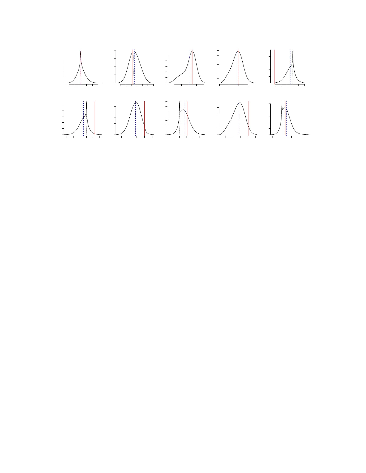
Loading high-quality paper...
Comments & Academic Discussion
Loading comments...
Leave a Comment