Random Walks, Electric Networks and The Transience Class problem of Sandpiles

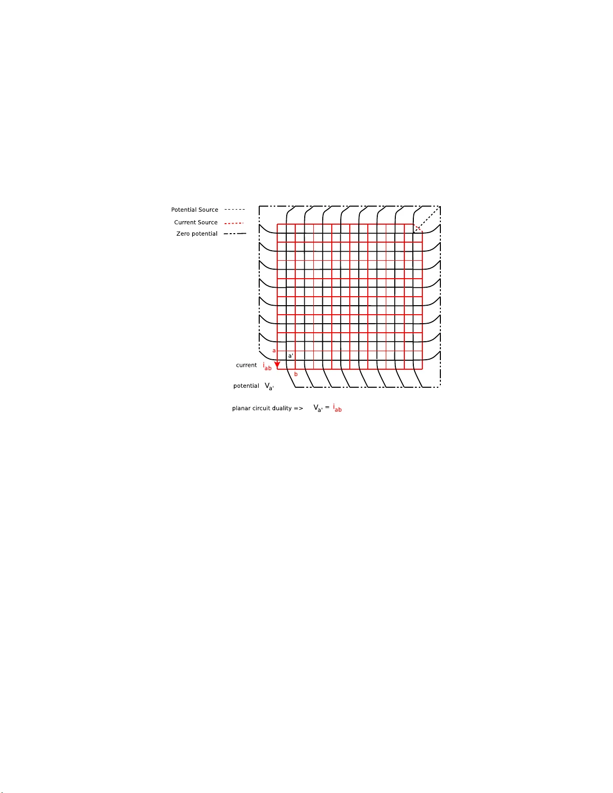
Random W alks, Electric Netw orks and The Transience Class pr oblem of Sandpile ∗ A yush Choure Sundar Vish w anathan Departmen t of Computer Science and Engineering Indian Institute of T ec hnology , Bom bay a yush, sundar@cse.iitb.ac.in Octob er 17, 2018 Abstract The Ab elian Sandpile Mod el is a discrete diﬀusion pro cess deﬁn ed on graphs (Dhar [15], Dhar et a l. [16]) whic h serv es as the standard model of self-or ganize d critic ality . The transience class o f a sandpile i s deﬁn ed as the maxim um num b er of particles t h at can b e added without making t he system recurrent ([4]). W e develo p the theory of discrete diﬀusions in contrast to contin uous harmonic functions on graphs and establish connections b etw een standard results in the study of random w alks on graphs and sandpiles on graphs. Using this connection and building other necessary machinery w e improv e the main result of Babai and Gorod ezky (SODA 2007,[ 2 ]) of the b ound on th e transience class of an n × n grid, from O ( n 30 ) to O ( n 7 ) . Pro ving that the transience class is small v alidates the general notion that for most natural phenomenon, the time during whic h the system is transient is small. F or degree b ounded gra ph s, w e demonstrate the ﬁrst constan t factor app ro ximation algorithm for th e transience class problem, b ased on harmonic functions. In addition, w e use the machinery developed to p ro ve a num b er of auxiliary results. W e give general u pper b ounds on the transience class as a function of the num b er of ed ges to the sink. W e exhibit an equiva lence b etw een tw o other tessellations of plane, the honeycomb and t riangular lattices. F u rther, for p lanar sandpiles we derive an explicit algebraic expression whic h prov a bly approximates th e transience class of G to within O ( | E ( G ) | ) . This expres- sion is based on the sp ectrum of the Laplacian of the dual of the graph G . W e also show a low er bound of Ω( n 3 ) on the transience class on the grid impro ving the obvio us b ound of Ω( n 2 ) . 1 In tro duction The ab elian sandpile mo del (ASM) is a t yp e o f diﬀusion proce s s deﬁned on graphs which is clos ely related to the chip ﬁring game inv estiga ted by Bjorner , Lov asz and Sho r [7] and T ardos [36]. Indeed s o me of the results in the mo del, proved by Bigg s [6], have an analog in the ASM of Dhar [15]. The mo del pro pose d by Dhar has b een studied in depth by the statistical physics communit y for inv estiga ting the pheno mena k nown as self-or ganize d critic ality in the dyna mics o f sa ndpile for mation. This for m ulation is known to b e closely related to other interesting a lbeit diverse pheno mena such a s stre s s distribution in earthquakes, size distr ibution in r aindrops, pa th length distributions in lo op-erased random w alks, for instance. F or a nice o verview, see the recent comprehensive survey article b y Dhar [14]. The ASM, thoug h easy to deﬁne, ha s a very pro found behavior and is far fro m b eing completely understo o d. Rese a rch in this area s tretc hes ∗ Extended draft appears i n [12] 1 across numerous disciplines suc h as probability theory , algor ithmics, theory of computing, combinatorics, non-linear dynamics, fractals, cellular automata, to name a few. These connections hav e b een b eautifully summarized by Kleb er in [26]. Dhar [14] also disc usses some generaliza tions o f the ASM like the Ab elian Distributed Pro cessor s (ADP) mo del which is used to mo del a grid o f a bstract state machines along with many theoretical and practical applications. In the standard sa ndpile mo del, “sand particles” are added at the vertices of a (multi) gr aph. A site (vertex) is stable as long as the num be r o f particles at the site remains less than its degree. A dding mor e pa rticles would render the site unstable and is accompanied b y the unstable site’s passing a particle alo ng each edge to its neig h b oring sites. This relaxation pro cess is referred to as t oppl ing . One of the sites known as the sink cannot topple. T o ensure that every relaxation pro cess even tually stabilizes, one needs the condition that the sink is rea c hable fro m every other site. A s the sys tem evolv es, the s andpile go es through a a sequence o f conﬁgura tio ns. Those which ca n b e r evisited in any toppling sequence are called r e curr ent , the remaining ones are termed tra nsient . T ypically , one starts with the empty conﬁg ur ation and as par ticles are added,o ne mov es through tran- sient co nﬁgurations till a recurrent conﬁgur ation is rea ched. Ther eafter the conﬁg urations stay recurr en t. The steady state b ehavior of a sandpile is characterized b y its set o f re- current s ta tes. It has bee n observed b y physicists that for most na tural phenomena, the time taken to reach a recurrent state is small. Hence any acceptable mo del must reﬂect this tendency to reach steady state rapidly and it b ecomes imp ortant to study the time taken to r each recur r ence in these mo dels. The essential parameter in our discussio n is the num ber o f par ticles which ensure recurrence. If particles a r e added randomly then a simple coup on collec to r type argument demonstrates p olynomial b ounds on the ex p e cte d time to r ecurrence (as already mentioned in [2 ]). The other scenario is to a dd particles adv er s ativ ely so as to avoid a r ecurrent state for as long as pos sible. This problem was highlighted b y Baba i and T o umpak ari [4] wher e they deﬁne the requisite n umber of particles as the tr ansienc e class of the sandpile. This later motiv ated the insightful work by Baba i and Goro dezky [2] on gr id based s andpile which a re the most studied ob jects as compared to any other gra ph class beca use of their outstanding signiﬁcance in statistical physics. In their path-breaking pap er, Babai and Goro dezky [2] sho w that for the standard n × n square g rid based sandpile, the maxim um n umber o f particles one can a dd befo r e hitting a recur ren t state is O ( n 30 ) . This is a remark able result in view of the fact that s ome clo sely related sandpile (for example line graph based) hav e transient state paths of length ex p onential in graph size. They use in trica te com binator ial arg umen ts based on particle conse rv ation and the s ymmetry g r oup of grid graphs to demonstrate the ab ov e men tioned b ounds. Howev er, s imulations suggest a b ound clo se to O ( n 4 ) for the grid sandpile. Also the questions raised requir e analys is of the problem in a more gener al setting. Our con tribution: W e be g in by showing a s trong connection b et ween the tra n- sience class problem of sa ndpile and ra ndom walks on the under ly ing gr aph. Using LP dualit y a nd basic r elaxation prop erties, w e derive bo unds on the tra ns ie nce class o f a sandpile in terms of harmonic functions over the underlying gra ph. Similarly , b ounds on sandpile imp edances acr oss any pair s of sites are o btained. These res ults fo rm the core of our ar g umen ts which contrast the discr e te mo del, sandpile, with the contin uous ver- sion; random walks. F o r degre e bo und sa ndpile, we use the indep endent set proper ties of no des with zero heights to demonstrate an alg orithm which approximates the transience class up to consta n t factors . The algorithm works by computing harmonic functions ov er graphs and signiﬁcantly tightens the connection b etw een sandpile and ra ndom walks o n the underlying gr aph. W e then prov e so me basic prop erties of sandpile a na logous to basic results in harmonic function theor y , for example o ccurrenc e of w or st case b ehavior at the bo undary , recipro cit y prop erties among any pair of sites, a nd so on. W e derive and use a triangle ine quality o f p otentials. This inequality provides suﬃcient ﬂexibility in a nalyzing the gr o wth r ates o f harmonic functions at the cost of lo osening the b ounds. W e use it 2 to o btain a b ound o n the cor ner to corner p oten tial res p onse on a grid net work. Using some symmetry prop erty of grids, we prove the main result of our pap er whic h improves the b ound on tra nsience cla s s from O ( n 30 ) (by Babai and Goro dezky [2 ]) to O ( n 7 ) . W e demonstrate a very gener al b ound on the tra nsience clas s in terms of sandpile size and the n umber o f co nnections to the sink. W e also show that in the case of planar sandpile, there exist explicit a lgebraic expressions which b ound the transience class v alues. These are based on the sp ectrum o f the Laplacian of planar dual of the given sa ndpile graph. W e derive the expres sion for grid sandpile and leav e it a s a (so mewhat technical) conjecture to establis h b ounds on its v a lue. W e believe that these would yield b o unds as low as O ( n 4 ) for this problem. In the last se c tion we discuss some impo rtant and interesting op en problems that would b e of interest to the theory comm unity . Our main contribut io n in this pap er is to bridge the ga p b et ween discrete diﬀusions on graphs and the theory of har mo nic functions on g raphs. Indeed, random walks, electric net works, gra ph spectra and LP duality have b een cent r al to ols in theo r etical computer science. W e ho p e that this pap er initiates a theory of discrete diﬀusions analo g ous to the celebra ted theory of mixing of Mar k ov chains. 1.1 Related W ork Random walks and Sandpile: W e beg in b y sketc hing a picture depicting an intui tive connection b etw een sandpile models and random w a lks on graphs . On a gr aph G ﬁx t wo vertices s and t . A simple random w a lk with a sp eciﬁed s tarting v ertex v involv es at each step, a choice of a neig h b oring vertex uniformly at rando m (See Bollobás [8] for a nice in tro duction). The p oten tial s π t ( v ) asso ciated with v , and s and t as p oles, is deﬁned as the probability of reaching t b efore s starting from v . Thes e π functions, discussed at length in the next section a re of par amount imp ortance in a nalytic po ten tial theor y (see, for instance [37]). With site s as the designa ted sink, add par ticles at site v and observe the r equisite num b er needed b efore a particle r eaches site t . F or a n y site which is ready to topple, if we lab el some par ticular par ticle among the set that are go ing to ﬂow out, then the pro babilit y that it lands up at a particular neighbor , is uniform among the neig hbo rs. If we add just enough particles at v , say N v , s o that exactly o ne par ticle reaches t , then the proba bilit y o f it being any pa rticular particle is uniform a nd the path it takes fro m v to t lo oks just like the ones co ns tituting s π t ( v ) . Infor mally s peaking , any particle in the starting pile a t v star ts a r andom walk at v which terminates at t or s , whichev er is encountered earlier . Intui tively , one expe cts that the pro babilit y s π t ( v ) would b e prop ortional to the recipro cal o f N v with the propo rtionality factor a ccoun ting for discreteness and storage at sites, features absen t in the usual netw ork theory axioms. Our main theorem for malizes this c o nnection and we der iv e as corollar ies some prop erties of sandpile whic h are discrete analogues of the corresp onding pr oper ties of r a ndom walks. Electric Netw orks: The class ical theory of electric netw orks alo ng with the well under - sto od connections with ra ndom w alks ([3 0], [17],[27]) has some very powerful and in tuitive results. These results hav e recently fo und applications in almost every impo r tan t area of theoretical computer science. Christia no, Kelner, Mądry and Spielman [11] hav e r ecen tly announced the fastest known algor ithm for computing approximate maxim um s − t ﬂows in capacita ted undirected g raphs. Using the electric cur rent ﬂows in this netw ork with s and t a s p oles, their algorithm constructs a pproximate ﬂows. Earlier Kelner and Mądry [22] used arguments ba sed on r a ndom walks to formulate the fastest known algo rithm for genera ting spanning trees from uniform distribution. Spielman a nd Sriv a sta v a [33] construct go o d sparsiﬁers of weigh ted graphs via a n e ﬃcient algorithm for computing a p- proximate eﬀective res istance b etw een any tw o vertices, a r esult which is quite insight ful on its own. The list of imp ortant results which use harmonic functions in a n essential manner go es on. The b eneﬁt of this co nﬂuence of resear ch in diﬀer en t clas sical a reas is indeed mutu a l. F or example, in their path br eaking pap er, Aror a, Ra o a nd V azira ni [1] give an O ( √ log n ) appr oximation algorithm for computing graph conductance. Our g oal 3 has b een to use the theory of harmonic functions in ana lyzing sa ndpile b ehavior (in the context of diﬀusion) in analog y with the theor y of r andom walks o n graphs. The results we rep ort in this pap er op en up the p ossibility o f analyzing thos e prop erties of ASM which may not hav e be e n p ossible using purely combinatorial ar gumen ts. Other Resul ts o n Sandpile: As already mentioned, resear c h problems on the ab elian sandpile model span acro ss numerous areas. Recent adv ances with a complexity theoretic ﬂav or include pro of of the one-dimensional sandpile predic tion problem in LOGDCFL b y Pet er Bro Milterson [28]. Also, Sch ulz [31] mentions a rela ted NP-complete problem. The g r oup structure of the s pace of recurrent co nﬁgurations, ﬁrst int r oduced by Dhar, Ruelle, Sen a nd V erma in [16], is also a fertile ar ea of analysis. Cori and Ros s in [13] show that sandpile gr oups of dual pla na r gr aphs are iso morphic. T oumpak ari [3 8] discusses some in teresting prop erties of sandpile groups o f r egular trees where ques tions related to group rank ar e studied and the pape r is concluded with an interesting conjecture on the rank of all Sylow subgr oups o f the sandpile group. Sp eciﬁc families of gr a phs like square cycles C 2 n , K 3 × C n , 3 × n t wisted bracelets, etc have been ana lyzed. W e r efer the reader to [21], [32], [2 0]. 2 Prelim inaries 2.1 In tro duction to the Ab elian Sandpile Mo del Our notation and termino logy follo ws B abai and Goro dezky [2]. Deﬁnition 1. A gr aph G is an ordered pair ( V ( G ) , E ( G )) where V ( G ) is called the set of vertices and E ( G ) is a s et of 2 − subsets of V , po ssibly with rep eated elemen ts, the set of edges. This is referred to as a m ulti-graph in literature but we will use graph for brev ity . The de gr e e of a vertex v ∈ V is deﬁned a s the num b er of edg es in E which contain v . T wo vertices v and u ar e ca lled adjac ent (or neighbor ing) if ( u, v ) ∈ E . A path b et ween tw o vertices u a nd v is an ordered sequence of edg es e 1 , e 2 , . . . , e k such that u ∈ e 1 , v ∈ e k and for a ll v alues of i , e i ∩ e i +1 6 = φ . The graph G is c onne ct e d if there exists a path betw een a n y pair o f vertices. T o mo del an Abelian Sandpile Mo del, we take a connected graph G with a sp ecial vertex called the sink , deno ted s ∈ V . No n- sink vertices in G are called or dinary v ertices and this subset will be denoted by V o = V − { s } . Deﬁnition 2. The c onﬁgur ation of a sandpile G is a map c : V o → N , whic h will be represented as a vector. The weight of c is | c | = P v ∈ V o c ( v ) . The c o nﬁguration c r ecords the num b er of s a nd particles contained in each of the ordinary sites. The empty conﬁgur ation is the zero vector. The c ap acity of a site is the maximum num b er o f pa rticles that it can hold and is one less then the degree of the no de. Deﬁnition 3. An ordinar y no de v is said to b e un stable in a conﬁgura tion c if c ( v ) ≥ degree(v). The co nﬁguration c is s a id to be unstable if a n y site under it is unstable, else it is referr ed to as stable. When a site is unstable it is sa id to topple , that is it pas ses on some of its par ticles to its neig h b ors. When a site v topples once, it loses degree (v) particles and each neighbor of v acquir es a particle for every edge commo n with v . The sink no de never topples. Starting with the empty conﬁgura tion, we keep adding pa rticles one by one on sites o f our choice a nd topple them when nec e s sary . The ASM evolv es in time thro ugh t wo mo des, par ticle a ddition at sites and relaxation of unstable sites v ia topplings. A toppling seq uence is an ordered set o f co nﬁgurations where every conﬁguration can be obtained from the previous o ne b y toppling some unsta- ble site in it. No te that the event of ma n y sites be c oming unstable simultaneously p o ses 4 no complication since the order in whic h they are subsequently rela xed do es not a ﬀect the ﬁnal stable conﬁgura tion that is obtained at the end of toppling sequence. Elementary pro ofs o f such co nﬂuence pr oper ties can be found in the pio ne ering pap er on ASMs by Dhar [15]. See also Babai and T oumpak ari [4]. Notation: W e write c 1 ≥ c 2 if ∀ v , c 1 ( v ) ≥ c 2 and c 1 ⊢ c 2 if there is a to ppling se q uence which tak es c 1 to c 2 . Finally we write, c 1 → c 2 if ∃ c 3 ≥ c 1 such tha t c 3 ⊢ c 2 . W e say that a c onﬁguration c 2 is r e achable from c 1 if c 1 → c 2 and u nr e achable other wise. In o ther words, one can add pa rticles to certain sites in c 1 so that there exists a toppling s e q uence leading to c 2 . Note that reachabilit y is transitive, i.e. c 1 → c 2 , c 2 → c 3 ⇒ c 1 → c 3 . Theorem 2.1 . ([15],[7]) Given any c onﬁgu ra tion c , ther e exists a unique st able c onﬁgu- r ation σ ( c ) such that c ⊢ σ ( c ) , indep endent of the chosen toppling se quenc e. Prop ert y 2.1. If c ⊢ σ ( c ) , then k c ⊢ kσ ( c ) Asso ciated with every toppling sequence is the count on the n umber of times each site has toppled, the vector o f toppling p otent ials , also r eferred to as the sc or e ve ctor in [2]. These toppling p otentials ar e very closely rela ted to the electr ic po ten tials tha t develop at v ario us no des when power s ource-sink a re appropr iately applied, a connection which we will discuss in detail in the coming sections . Deﬁnition 4. As s uming c 1 ⊢ c 2 , the toppling potential function z c 1 ,c 2 : V 0 → N is deﬁned as z c 1 ,c 2 ( v ) : the n umber of times v toppled in a toppling sequence from c 1 to c 2 . W e deno te z c,σ ( c ) b y z c . This function is well deﬁned a s the num b er of times a particula r site topples is inde- pendent of the toppling sequence chosen, already noted in [2]. The pro o f employs the fact that the principa l minor of a connected g raph’s com binator ial laplacian is of full rank. A co nﬁguration is called r e cu rre nt if it is reachable from any co nﬁguration. As a lready men tioned, we say that a c o nﬁguration c i is reachable fro m a conﬁguration c j if b y adding some particles to c j (po s sibly at multiple sites ) a nd subse q uen tly relaxing it, we ca n obtain c i . A co nﬁg uration is tr ansient if it is not r ecurrent. The set of recurre nt conﬁgurations is therefore, close d under reachabilit y . Prop ert y 2.2. If ∃ c ′ such that ther e is a toppling se qquenc e fr om c ′ to c in which every site has topple d at le ast onc e, then c is r e curr ent. The pro of fo llows fro m the fact that the existence of such a to ppling sequence precludes the existence o f forbidden sub-co nﬁgurations and hence makes the conﬁguration recurrent. F or a complete discussion on forbidden sub-conﬁgurations a nd recurr ence of co nﬁgurations the reader is refer red to [15] and [14]. W e analyze the pro cess of adding one gra in at a time to the sa ndpile a nd study its evolution. As in the standar d theory of Marko v chains, recurrence characterizes the long term (steady state) b ehavior of sandpiles. Our inv estiga tion is concer ned with the maximum n umber of particles that ca n b e added while staying transient. F ollowing Babai and Goro dezky [2], for a sandpile S we deﬁne, Deﬁnition 5. The tra nsienc e class of S deno ted b y tcl( S ), is deﬁned as the ma xim um n umber o f particles that can b e added to S b e fo re reaching a r ecurrent conﬁgura tion. In view o f prop erty 2.2, w e can bound the transience class from ab ov e by the maximum numb er of p articles that c an b e add e d b efor e al l the n o des have topple d at le ast onc e . Showing that this b ound is tight upto co nstan t factor s is also not very hard. W e defer a fuller disussion of q ues tions of this nature to our subsequent man uscr ipt. 5 2.2 Basics of Harmonic F unctions and P otential Theory F or a very nice introduction to harmonic functions on gr aphs, w e r efer the r e ader to the bea utifully written pa per by Benjamini a nd Lov as z [5] and to T elcs [37] for a thoroug h view. W e sta rt with so me imp ortant deﬁnitions and fundamen ta l prop erties. Given a connected graph G and a function π : V ( G ) → R , we say that π is harmonic over V h if, 1 deg r ee ( v ) X u ∼ v π ( u ) = π ( v ) v ∈ V h (1) The remaining vertices (lying in V − V h ) are ca lled the “po les” of π . The set V h is also ca lled the interior of π with vertices a djac e nt to the set of p oles referred to a s the b oun dary . W e se e that the v alue of π at any vertex in V h is the av er age of its v alue in the immediate neighborho o d. In cas e of multi gra phs, we tak e the appr opriate weigh ted means, where the weights are the num b er of co mmon e dg es. This lea ds us to the ﬁrs t basic prop erty , Prop ert y 2. 3. A ny non-c onstant harmonic fun ction c an assume its ex t r eme values only at the set of p oles. It follows that every non-co nstan t harmonic function has at least tw o p o les, its maxima and minima. Such functions ar e completely determined by their v alues on these vertices. F orma lly sp eaking, Prop ert y 2.4. Uniqueness: If t wo functions harmonic on V h agr e e on t he b oundary, they agr e e everywher e in t he int erior. More gener a lly , w e have the following prop erty , Prop ert y 2. 5. Given a set of p oles, a harmonic fun ct ion is uniquely determine d mo dulo sc aling and tr anslation by a c onstant. Prop erties 2.4 and 2.5 imp ortant as they allow one co nsiderable freedom in construct- ing ha rmonic co mpletions of functions deﬁned over the bo undary set. This pro blem is the discrete a nalogue of the classica l b oundary v alue pro blems in complex ana ly sis. W e will describ e tw o imp ortant exa mples in whic h these function ar ise na turally , R andom W alks on Gr aphs: Consider a gr a ph G and t wo sp ecial v er tices s and t . The po ten tial asso ciated with v , with s and t a s p oles, s π t ( v ) is deﬁned a s the proba bilit y of rea ching t befor e s starting from v . One ca n check that the function π so deﬁned is indeed harmonic o n the s e t V − { s, t } , with the maximum v a lue of 1 a t the no de t and the minimum v alue 0 at s . The g e neralization to the multi-pole s itua tio n is als o straightforw ar d. Ele ctric N etworks: Consider a resistive electric netw ork (i.e. a circuit made up entirely of r esistors). Let s π t ( v ) be the p oten tial that a pp ears at no de v when unit p otential is applied across t and s . Using the e q uation of charge conserv ation (Kirchoﬀ ’s no de law), one can show that these p oten tials a re harmonic on all no des e x cept s and t . The main implication here is that one can intuitiv ely think of the electric netw ork the- ory as an analysis of rando m walks o f electrons on the underlying graphs. Consequently , results from netw or k theory can b e used to pr o ve interesting fac ts in other r elated ar - eas. As a n exa mple, co nsider the problem of constructing the harmo nic completion of a function with given b oundary v alues. All one needs to do is to take the cor resp onding circuit and a pply po ten tials equal to the b oundary v alues o n the b oundary p oints. The po ten tials that will app ear on other nodes ca n b e computed using basic linear algebra (the only non-trivial step inv olves inv erting the combinatorial Laplacian o f G ) thus allowing construction of harmonic completions eﬃciently . W e outline b elow three very basic and fundamen tal r e s ults of netw ork analysis which will b e needed in the following sectio ns . 6 Theorem 2. 2. Sup erp osition Principle: The su p erp osition principle states t hat for al l line ar systems, the net re sp onse at a given plac e and time c ause d by two or mor e stimuli is the sum of the r esp onses which would have b e en c ause d by e ach stimulus individual ly. Theorem 2.3. Comp ensation The or em: If the imp e danc e Z of a br anch in a network in which a curr ent I ﬂ ows is change d by a ﬁnite amount d Z , then the change in t he curr ents in al l other br anches of the network may b e c alculate d by inserting a voltage sour c e of − I d Z into that br anch with al l other voltage sour c es r eplac e d by their internal imp e danc es. Theorem 2.4. R e cipr o city The or em: In its simplest form, the r e cipr o city the or em states that if an emf E in one br anch of a r e cipr o c al network pr o duc es a curr ent I in another, then if the emf E is m ove d fr om the ﬁ rst t o the se c ond br anch, it wil l c ause the same curr ent in the ﬁrst br anch, wher e the emf has b e en r eplac e d by a short cir cuit. Any network c omp ose d of line ar, bilater al elements (such as R, L and C) is re cipr o c al. The recipro cit y theorem can be restated in terms of just p otential sources and p oten- tial mea suremen ts using the notion of eﬀective resistances b et ween pairs of no des. The eﬀectiv e resistance b e tw een a pair of nodes u and v , R ef f ( u, v ) is deﬁned as the potential diﬀerence which dev elops b etw een u and v if a unit current source is applied across u and v . Lemma 2. 1 . Potential R e cipr o city L emma : If taking s and t as p oles with π ( s ) = 0 and π ( t ) = 1 induc es a p otential of s π t ( v ) at no de v and inter changing the r oles of v and t induc es s π v ( t ) at t then, R ef f ( s, t ) s π t ( v ) = R ef f ( s, v ) s π v ( t ) (2) Pro of : Consider the given netw or k G with the sp e cial no de s ∈ V ( G ) . W e refer to the cor respo nding mo diﬁed netw ork G ( ǫ ) obtained fro m G by a dding an edge with resistance 1 / ǫ be tw een every no de and s . In particular, G (0) ≡ G . F urthermore, w e refer to a n edge b etw een s and u by ˜ su . W e will b e using the c urrent source version of the recipro city theorem. If applying a unit cur ren t s ource across ˜ st results in a p otential o f v acr oss ˜ sv , then applying unit curr en t source acro s s ˜ sv results in a p otential of v units across ˜ st . The v alue of this po ten tial v c a n b e expres sed, using Ohm’s law, as the ra tio of current thro ugh the edge and the r esistance of the ǫ − edg e betw een the particular no de and sink. Since bo th po ten tials ar e equa l in magnitude, we can say that on G ( ǫ ) , R ef f ( s, t ) s π t ( v ) = R ef f ( s, v ) s π v ( t ) This follows from observing that applying a unit curr en t source across ˜ sv is equiv alent to applying a voltage source o f R ef f ( s, v ) acr oss ˜ sv . Because of linea rit y , it follows that a po ten tial of s π v ( t ) R ef f ( s, v ) . app ears at no de t . Similarly so for the other co nﬁguration. This equation holds fo r ar bitrarily small v a lues of ǫ . Consequently it holds for gr a ph G (0) .  In particular, when the eﬀective resistances acro s s s and t a re the s ame as s and v , we hav e s π t ( v ) = s π v ( t ) . In the following discussion, we will omit the left s ubscript ( s ) from s π t whenever it is cle a r from co n text. W e s a y that a walk P is an instanc e of s π t if it star ts at some vertex v , av oids s and ends a t t . The following lemma may alr eady be k no wn to exper ts. Since we co uld not ﬁnd it in litera tur e , w e present it with a simple pro of. Lemma 2 .2. A triangle ine quality for p otentials π i ( j ) .π j ( k ) ≤ π i ( k ) (3) 7 Pro of : Let P ( k , j ) b e the set of all w alks from k to j av oiding s . This set can be partitioned in to tw o comp onents, namely the walks passing throug h i and the ones av oiding it, denoted by P i ( k , j ) a nd P ¯ i ( k , j ) r espec tively . F or any walk P which is an instance of π i , let the pro babilit y of o ccurrence b e π i ( P ) . Then by deﬁnition, π j ( k ) = X P ∈P i ( k,j ) π j ( P ) + X P ∈P ¯ i ( k,j ) π j ( P ) Similarly , π i ( j ) = X P ∈P ( j,i ) π i ( P ) Using these tw o rela tions, we obtain π i ( j ) .π j ( k ) = X P ∈P ( j,i ) π i ( P ) . X P ∈P i ( k,j ) π j ( P ) + X P ∈P ( j,i ) π i ( P ) . X P ∈P ¯ i ( k,j ) π j ( P ) (4) Consider the ﬁrst term on rig h t side in equation (4). Being a probability measure, the v alue of P P ∈P ( j,i ) π i ( P ) is bo unded a bove by 1 . Every s -avoiding walk from k to j passing through i can be deco mposed into t wo comp onents, a walk from k to i av oiding j and a walk fro m i to j . This implies, P P ∈P i ( k,j ) π j ( P ) = P P ∈P ¯ j ( k,i ) π i ( P ) . P P ∈P ( i,j ) π j ( P ) ≤ P P ∈P ¯ j ( k,i ) π i ( P ) . The ﬁr st term therefore has the following b ounds, X P ∈P ( j,i ) π i ( P ) . X P ∈P i ( k,j ) π j ( P ) ≤ X P ∈P ¯ j ( k,i ) π i ( P ) (5) F or b ounding the seco nd term, obs e r v e that any s -avoiding walk fro m k to i which passes throug h j , can b e treated a s a juxtapo s ition of a walk from k to j , a voiding i , a nd a walk from j to i . Hence, X P ∈P ( j,i ) π i ( P ) . X P ∈P ¯ i ( k,j ) π j ( P ) = X P ∈P j ( k,i ) π i ( P ) (6) Using equatio ns 4, 5 and 6 we get π i ( j ) .π j ( k ) ≤ X P ∈P j ( k,i ) π i ( P ) + X P ∈P ¯ j ( k,i ) π i ( P ) = π i ( k )  R emark: The utilit y of this inequality b ecomes clear w hen interpreted in the co n text of electric netw o rks. Consider a netw ork such that the no de with gro und po ten tial is ﬁxed and w e are allowed to apply p ow er a t any other no de and obser v e the res ulting p otentials. The inequalit y implies that if applying a po tential V 1 at i pro duces unit potential at no de j and a pplying V 2 at no de j pro duces unit potential at no de k , then applying V 1 .V 2 units at i pro duces at le ast unit p otential a t no de k . 3 Reducing the transience class problem to estimating harmonic functions o v er graphs W e ﬁrst consider the single site particle addition strategies . W e will later show that the eﬀect of a llo wing par ticle addition a t multiple sites o n our tra nsience clas s estimates is inconsequential as far as our estimates are concerned. 8 Deﬁnition 6 . Co nsider a sandpile S with no des u and w . The sandpile imp e danc e of the o rdered pair ( v, w ) , R s ( v , w ) is deﬁned as the maximum num b er of particles that one can add at v b efore a toppling at w o ccurs. Note tha t unlike the imp edance of electr ic netw ork s , sandpile imp edance is not sym- metric in its arguments, i.e. in g eneral R s ( v , w ) 6 = R s ( w, v ) . T o estimate its v alue, we in tro duce the following LP rela xation. max x v 0 ≤ X v ′ ∼ v z ( v ′ ) − d ( v ) .z ( v ) + x v ≤ d ( v ) − 1 ∀ u 6 = v : 0 ≤ X u ′ ∼ u z ( u ′ ) − d ( u ) .z ( u ) ≤ d ( u ) − 1 z ( w ) ≤ 0 , z ≥ 0 , x ≥ 0 The v alues of x v (the n umber of particles added a t v ) and z (the vector of toppling counts) that are rea lized ab ov e are a feasible solution of this LP and hence the optimum of this LP yields an upp er bo und on the R s ( v , w ) . With the ﬁxed sink no de, s , we deﬁne π w ( v ) as the p otent ial a t no de v when a unit po ten tial is applied at no de w . In terms o f these po ten tial functions, the following bound holds. Lemma 3. 1 . The optimum value of the ab ove LP is b ounde d fr om ab ove by t he fol lowing value, 1 π w ( v ) X u ( d ( u ) − 1) .π w ( u ) (7) Pro of: W e consider the fo llowing relaxed version of the given L P . max x v X v ′ ∼ v z ( v ′ ) − d ( v ) .z ( v ) + x v ≤ d ( v ) − 1 ∀ u 6 = v : X u ′ ∼ u z ( u ′ ) − d ( u ) .z ( u ) ≤ d ( u ) − 1 z ( w ) ≤ 0 , z ≥ 0 , x ≥ 0 F rom the weak dualit y for LPs, it follows that to obtain an upp er b ound of α on the optim um v alue of the ab ov e system, it suﬃces to ﬁnd a feasible solution of the dual LP of v alue α . The dual is the following : min X u ( d ( u ) − 1) .Y ( u ) X u ′ ∼ w Y ( u ′ ) + Y ′ − d ( w ) .Y ( w ) ≥ 0 ∀ u 6 = w : X u ′ ∼ u Y ( u ′ ) − d ( u ) .Y ( u ) ≥ 0 Y ( v ) ≥ 1 , Y ≥ 0 , Y ′ ≥ 0 Consider the following set of equations X u ′ ∼ w Y ( u ′ ) + Y ′ − d ( w ) .Y ( w ) = 0 (8) ∀ u 6 = w : X u ′ ∼ u Y ( u ′ ) − d ( u ) .Y ( u ) = 0 (9) Y ( v ) = 1 9 A non-negative set of v alues satisfying the ab ov e set is fea s ible for the dual LP . W e ﬁnd these by considering the resistive circuit b S , obtained by replacing each edge in S by a unit resistance. W e a s sign g round po ten tial to the sink, and inject cur r en t at no de w such that it gets unit p otential. The p otential that develops on any no de u is s π w ( u ) . The po ten tial v alue at no de v , π w ( v ) , ca n be us ed to scale the input current a t w thereb y scaling all the po ten tials as well, such that p otential at no de v bec omes unit. It follows that the v alues Y ( u ) = π w ( u ) /π w ( v ) a nd Y ′ equaling the v a lue of the curr en t injected form a feasible solution of the dual LP . The ob jectiv e v alue at this p oint is, 1 π w ( v ) X u ( d ( u ) − 1) .π w ( u )  This yields an upper b ound on x v . T o obtain a low er bound, consider the co mplemen- tary problem of ﬁnding x ′ v , the minimum num b er o f particles that m ust be added at v to observe a toppling at w . The following LP’s ob jective v alue forms a low er bo und on x ′ v , min { x ′ v } 0 ≤ X v ′ ∼ v z ( v ′ ) − d ( v ) .z ( v ) + x ′ v ≤ d ( v ) − 1 ∀ u 6 = v : 0 ≤ X u ′ ∼ u z ( u ′ ) − d ( u ) .z ( u ) ≤ d ( u ) − 1 z ( w ) ≥ 1 , z ≥ 0 , x ≥ 0 The pro of of the following lemma is analog ous to the previous cas e. Lemma 3. 2 . The optimum value of the ab ove LP is b oun de d fr om b elow by the fol lowing value, 1 π w ( v ) (10) Pro of: Consider the relaxed version of the ab ov e LP , min { x ′ v } X v ′ ∼ v z ( v ′ ) − d ( v ) .z ( v ) + x ′ v ≥ 0 ∀ u 6 = v : X u ′ ∼ u z ( u ′ ) − d ( u ) .z ( u ) ≥ 0 z ( w ) ≥ 1 , z ≥ 0 , x ≥ 0 F rom the w eak dua lit y for LPs, it follo ws that to obtain a lower b ound on the optim um v alue of the ab ov e system, it suﬃces to ﬁnd a feasible solution of the dual LP . The dual is the following : max Y ( w ) X u ′ ∼ w Y ( u ′ ) + Y ′ − d ( w ) .Y ( w ) ≤ 0 ∀ u 6 = w : X u ′ ∼ u Y ( u ′ ) − d ( u ) .Y ( u ) ≤ 0 Y ( v ) ≤ 1 , Y ≥ 0 , Y ′ ≥ 0 10 Consider the following set of equations X u ′ ∼ w Y ( u ′ ) + Y ′ − d ( w ) .Y ( w ) = 0 (11) ∀ u 6 = w : X u ′ ∼ u Y ( u ′ ) − d ( u ) .Y ( u ) = 0 (12) Y ( v ) = 1 As b e fore, any non-neg ative set of v alues satisfying the ab ov e system is feasible for the dual LP , and therefore for ms a low er bo udn on the ob jective v a lue. W e ﬁnd these b y co nsidering the resistive circuit b S , o btained by r eplacing ea c h edge in S by a unit resistance. W e a ssign g round p otential to the sink, and inject current at no de w suc h that it gets unit po ten tial. The p otential that develops on any no de u is s π w ( u ) . The po ten tial v alue a t no de v , π w ( v ) , can b e used to s cale the input current a t w thereby scaling all the po ten tials as well, such that p otential at no de v bec omes unit. It follows that the v alues Y ( u ) = π w ( u ) /π w ( v ) a nd Y ′ equaling the v a lue of the curr en t injected form a feasible solution of the dual LP . The ob jectiv e v alue at this p oint is π w ( v ) − 1 .  Clearly the maximum n umber of particles that can be added at v b e fore toppling some w is just o ne less then the minim um num b er that need to be added a t v to topple w , that is x ′ v = x v + 1 . Using eq uations (7) and (10), the following tw o- sided b ounds are obtained. 1 π w ( v ) − 1 ≤ x v ≤ 1 π w ( v ) X u ( d ( u ) − 1) .π w ( u ) (13) F urther, deﬁne the p otential pr oﬁle o f the cir c uit when unit p otential is applied at no de w as Γ S ( w ) = X v ( d ( v ) − 1) .π w ( v ) Using this notation, R S ( v , w ) = x v satisﬁes the following genera l b ounds. Lemma 3 .3. R s ( v , w ) is O (Γ S ( w ) .π w ( v ) − 1 ) . Lemma 3 .4. R s ( v , w ) is Ω( π w ( v ) − 1 ) . T o ﬁnd the maximum num b er o f particles one can add at v b efore every other site topples, o ne simply needs to co nsider the maximum v alue of R S ( v , w ) over all v alues o f w ∈ V o . Consequently , o ne ca n ﬁnd the maximum num ber of particles that ca n b e a dded at a single site b efore every other site topples, b y considering the maximum of R S ( v , w ) ov er all pairs ( v , w ) . This v alue, max v, w { Γ S ( w ) π w ( v ) − 1 } , also for ms a b ound on tcl ( S ) as allowing particle addition a t multiple sites ab ov e gives the same estimates. This fact follows fro m essentially the same line of a rgument that was used for ﬁnding the upp er bo unds except that in this case instead of x v , the o b jective function to maximize is P u x u where x u is the num b er of pa rticles added at u . Theorem 3.1. tcl ( S ) is O (max v, w { Γ w ( S ) π w ( v ) − 1 } ) . As each of the π w ( v ) lies b et ween 0 and 1 , the v alue of Γ w ( S ) is there fore b ounded betw een 1 and | 2 E ( S ) | . Hence, we hav e the following relaxed upp er bo und on the v a lue of tcl ( S ) , Lemma 3 .5. tcl ( S ) is O ( | E ( S ) | . ma x v, w { π w ( v ) − 1 } ) . 11 These results q ua n tify the relationship betw een sandpiles and random walks o n graphs. How ever, the theory of p otent ial functions o n gr aphs b oas ts o f s ev er a l very intuitiv e and bea utiful r esults, e.g . the r ecipo city theorem. In a later section, w e show that the parallelism b et ween sandpiles a nd electric netw orks runs deep er by demons trating the sandpile versions of some w ell known basic r esults in netw o rk theory . W e star t by co nsidering some simple prop erties of p oten tial funtions. F o r exa mple, consider the pr oper t y 2.3 whic h says that the maximum and minimum o f p otential func- tions o ccur at p oles. An elementary pro of by c o n tradictio n is easily conceiv able. In the case of sa ndpiles, one can think of a similar no tio n of maxima/ minima in terms of ease o f per colation o f particles. When we add particles anywhere (may b e more than one site), then is it so that the last site to topple will b e adjacent to s i nk? Or co nsider the dual problem. W e a r e allow ed to a dd particles at one site only . F or any pa rticular site whos e toppling we wish to delay for as long as p ossible, is it true that the b est strategy is to add pa rticles at a site adjacent to s ink? T o r ephrase, is it true that for any site w , the v alue o f R S ( v , w ) is maximized for some v adjacent to the sink? Note that b oth these questio ns are t wo sides of the sa me coin in case o f random w alks bec a use o f the recipro city prop erties discussed ab ov e. The ﬁrs t ha s a dir ect analogy for sandpiles. Lemma 3 .6. The last site to topple is always adjac ent to sink. Pro of : Assume that the last site to to pple is not adjace nt to sink. S ince each of its neighbors has alr eady toppled, it ha s received at least as many particles as its degree and has b ecome unstable at least once co n tradicting the a ssumption that the par ticular site has never toppled.  W e now ﬁx the site under observ ation and ask the same question ab out the s ite where we add par ticles. Lemma 3. 7. F or a given w , the estimate of R s ( v , w ) is maximum when v is at b oundary. Pro of :F or a ﬁxed w , the v alue of Γ S ( w ) is ﬁx e d. One has to show that the v alue of π w ( v ) is minim um for some vertex v adjacent to sink, s . This clearly follows from the fact that for every internal no de u , π ( u ) is a c on vex combination, in particular the weight ed arithmetic mean, of the π ( . ) v a lues at its neighbor s. This means that π ( u ) is b ounded betw een the v alues s panned by the neighbors, so it ca nnot be an extreme p oin t.  Note: This lemma talks ab out the estimate and n ot the e x act v alue of R s ( v , w ) . The lemmas prove that while using the Theo rem 3.1, it is enough to consider b oth sites on the b oundary set (i.e. adjacent to sink). The following lemma is the s a ndpile analog ue of the classica l p otential r ecipro cit y lemma fro m net work theo ry . Lemma 3 .8. Sandpile R e cipr o city lemma : If adding p p articles at v c auses toppling at w then adding 2 | E ( S ) | R ef f ( v, s ) R ef f ( w, s ) .p p articles at w c auses a toppling at v . Pro of : Using theorem 3.3, the ratio of R S ( v , w ) to R S ( w, v ) can b e b ounded. R S ( w, v ) R S ( v , w ) ≤ max R S ( w, v ) min R S ( v , w ) = π v ( w ) − 1 . Γ( v ) π w ( v ) − 1 ≤ 2 | E ( S ) | . R ef f ( v , s ) R ef f ( w, s ) Where the last inequalit y follows fro m the p otential r ecipro cit y men tioned in Lemma 2.1. Given p = R S ( v , w ) , we get the required b ound on R S ( w, v ) in ter ms of p .  One can go even further by using the fact that the maximum v alue of R ef f is | V ( s ) | (attained for paths) and minimum v alue is at lea st 1 / | E ( S ) | (attained for just a pair of adjacent no des with many parallel edes b et wene them). B abai and Go ro dezky [2] conjectured the following. 12 Conjecture 1. ([2])Assume that for sandpile χ , the induc e d sub-gr aph on the set of or dinary vertic es is c onne cte d. Then t he tr ansienc e class of χ (the lar gest weight of any tr ansient c onﬁgur ation) is the height of the tal lest tr ansient stack of gr ains plac e d on a single site. The co njecture is equiv alent to sa ying that using s ing le site particle addition strategies one can attain the transience cla ss b ounds. How ever this is not so . A counter-example b y Sunic app ears in [4]. W e present a simpler co un terexample and an intui tive reason why this conjecture is false in general. Assume that in a sandpile χ with ﬁnite tr ansience class, one can attain the bounds b y adding particles a t the single s ite v a nd w topples last. After the last pa rticle is added, adding one more is supp osed to make the co nﬁguration recurrent. Whic h means this heaviest transient conﬁguration, when relax e d should have every site ﬁlled to its maximum capacity , ex cept for w which has not yet toppled and contains pa rticles less then the maximum capa cit y . If there exists some other site which is not ﬁlled up to maximum capacit y , o ne can add particles ther e and ﬁll it up (only till it stays s ta ble, of co ur se). Hence the v alidity of conjecture res ts on the ra ther unlikely premise that in the heaviest transient conﬁgura tion, every site but one is ﬁlled to its maximum stable capacity . A condition which one would think unlikely when ther e are no symmetries in χ (trivial automo rphism g roups). W e will present an exa mple with non-trivial s ymmetries to demonstrate that even in this case, o ne cannot exp ect such a strong prop erty . Consider the grid s andpile χ n with n = 4 . W e add par ticles at the top left corner. As exp ected, the last site to to pple is the b ottom right corner . Her e is the stable conﬁgura tion corresp onding to the heaviest transient conﬁgur ation with a s ta c k of particles placed on the top left. 3 3 3 0 3 0 3 2 3 3 2 3 0 2 3 2 All the sites which have fewer then 3 particles , can b e topp ed up without inducing a toppling a t the bo ttom r ight corner no de, and then adding a particle at top left corner induces r ecurrence. This demonstrates that single site par ticle addition do not work for this pair. W e discuss a related op en question in the section o f future w or k. 4 A constan t factor appro ximation for transience classes of degree b ounded graphs W e will now arg ue that in the case of degree b ound gr aphs, using some combinatorial prop erties o f indep enden t sets in sa ndpile g r aphs along with arg uments similar to the ones outlined in the previo us sec tio n for the lo wer bound der iv ed in Lemma 3.2, one can derive tight (up to consta n t factors) low er b ounds for the transience classes. In the sandpile S , let x ′ v be the minimum num b er of particles that ca n need to be added at no de v such that the no de w topples at least once. Clear ly x ′ v = x v + 1 . As in the pr evious section, the following LP relaxation forms a lower b ound on the v alue of x ′ v . min x ′ v 0 ≤ X v ′ ∼ v z ( v ′ ) − degree ( v ) .z ( v ) + x v ≤ degree ( v ) − 1 ∀ u 6 = v : 0 ≤ X u ′ ∼ u z ( u ′ ) − degree ( u ) .z ( u ) ≤ deg r ee ( u ) − 1 z ( w ) ≥ 1 , z ≥ 0 , x ′ v ≥ 0 13 Consider the scenar io in which we add x ′ v particles a t v and allow the conﬁguration to settle down to sta bility . F urthermore, let the nu mber of par ticles that a ppear at a n y no de u in the resulting stable conﬁgura tion be h u . The following lemma g iv es a low er bo und on the particle co un t x ′ v in terms of these height functions h u . Lemma 4.1. The value of the p article c ount x ′ v is b oun de d fr om b elow by the fol lowing value, 1 π w ( v ) X u h ( u ) .π w ( u ) (14) Pro of: Clearly 0 ≤ h u ≤ degree ( u ) . In the linear progr a m stated ab ov e, replacing each pa ir o f constra in ts o f the type 0 ≤ P v ′ ∼ v z ( v ′ ) − d ( v ) .z ( v ) + x v ≤ d ( v ) − 1 b y P v ′ ∼ v z ( v ′ ) − d ( v ) .z ( v ) + x v = h v , ma in tains the prop erty that the optimum v alue is at least a low er bo und to the exact so lution to the particle count x ′ v . The altered LP is the following, min x ′ v X v ′ ∼ v z ( v ′ ) − degree ( v ) .z ( v ) + x ′ v = h ( v ) ∀ u 6 = v : X u ′ ∼ u z ( u ′ ) − degree ( u ) .z ( u ) = h ( u ) z ( w ) ≥ 1 , z ≥ 0 , x ′ v ≥ 0 T o b ound the o ptimum v alue, w e will consider the dual of this minimiza tio n pro gram and ﬁnd a suitable feasible p oint . The v alue of the cost function at that p oin t will b e used as b ound. The dua l is the following maximization progra m. max Y ′ + X u h ( u ) .Y ( u ) X u ′ ∼ w Y ( u ′ ) + Y ′ − degr ee ( w ) .Y ( w ) ≤ 0 ∀ u 6 = w : X u ′ ∼ u Y ( u ′ ) − degree ( u ) .Y ( u ) ≤ 0 Y ( v ) ≤ 1 , Y ≥ 0 , Y ′ ≥ 0 As in the previous lemma, we consider the following s et of equations, whose fea sible region is inside the one corre sponding to the dua l we mentioned ab ove. X u ′ ∼ w Y ( u ′ ) + Y ′ − d ( w ) .Y ( w ) = 0 ∀ u 6 = w : X u ′ ∼ u Y ( u ′ ) − degree ( u ) .Y ( u ) = 0 Y ( v ) = 1 A non-negative set of v alues satisfying the ab ov e set is fea s ible for the dual LP . W e ﬁnd these by considering the resistive circuit b S co rresp onding to the gra ph S (with each edge having unit resistance). The sink no de is ass ig ned ground p o ten tial and just enough current is injected at no de w s o that it attains unit p otential. In terms of the sta nda rd po ten tial functions describ ed earlier, the potential that develops on any no de u is s π w ( u ) . The po ten tial v alue at no de v , π w ( v ) , ca n be us ed to scale the input current a t w thereb y scaling all the po ten tials as well, such that p otential at no de v bec omes unit. It follows 14 that the v alues Y ( u ) = π w ( u ) /π w ( v ) a nd Y ′ equaling the v a lue of the curr en t injected form a feasible solution of the dual LP . The ob jectiv e v alue at this p oint is, Y ′ + 1 π w ( v ) X u h ( u ) .π w ( u ) Since the curren t, Y ′ , is a p ositive quantit y , the ab ov e deriv ation implies the Lemma.  W e will now sho w that the low er bo und is at most a constant factor smaller then the upper b ound. W e start with deﬁning a n auxiliary set of v aria bles ˆ h v such that, ˆ h v = 1 ≡ h v ≥ 1 F rom the pos itivity of π ( . ) function and the domination r e lation ˆ h v ≤ h v , the follo wing inequality follows. b Γ = 1 π w ( v ) X u ˆ h u .π w ( u ) ≤ 1 π w ( v ) X u h u .π w ( u ) (15) W e will now b ound the v a lue b Γ from b elow. Lemma 4.2. (Dhar [14], Bab ai and Gor o dezky [2]) In any stable r e curr ent c onﬁgur ation, for every e dge, b oth the incident vertic es c annot have zer o p articles. This follows from the fact that in a ny stable recurr en t conﬁgura tio n, the last toppling of one of them would hav e taken place after the other a nd so the seco nd no de nece s sarily has at least one particle. F o r every edge u , v , at least one o f h u and h v is ≥ 1 . Corollary 4. 1. The set of no des I = { v : h v = 0 } form an indep endent set. Assume further that the gr aph satisﬁes ( ∆ ), i.e. the maximum degre e is ∆ . Using this we will obtain the required bo unds. Consider any vertex v ∈ V h along with its neighborho o d (see ﬁgure (1)). The function π ( . ) is harmonic ov er this neighbo rho o d, so we hav e degree ( v ) π ( v ) = X u ∼ v π ( u ) from which w e get the sum of π ( . ) ov er any neigh b orho o d in V h as, π ( N ( v )) = π ( v ) + X u ∼ v π ( u ) = ( degree ( v ) + 1) π ( v ) The contribution of any lo cal r egion in the restricted p otential trace b Γ dep ends o n just tw o p ossibilities regar ding h v . W e deal with them s eparately . - Case h v = 0 : v ∈ I , consequently none of its neig hbo rs are in I . In this case the contribution to b Γ is the s um P u ∼ v π ( u ) = degree ( v ) π ( v ) = degree ( v ) degree ( v )+1 π ( N ( v )) . - Case h v = 1 : v / ∈ I , and so me of its neighbo rs are in I . Assume the worst case scenario when a ll the neighbors are in I . The cont ribution to b Γ in such a situation is just π ( v ) = 1 degree ( v )+1 π ( N ( v )) . 15 Center node selected Center node’s neighbors selected Figure 1: Neighbor hoo d aro und vertex v ; tw o cases, v selected and not selected in I It follows that any neighborho o d N ( v ) contributes at le a st 1 degree ( v )+1 π ( N ( v )) to b Γ , regar dles s o f the sp eciﬁc v alues of h v . Since the degre e is b ounded by ∆ , this transla tes to a minimum contributi o n of 1 ∆+1 π ( N ( v )) . Therefore, the v alue of b Γ in equation (15), for any independent set I , is at least 1 (∆ + 1) π w ( v ) X u π w ( u ) (16) The upp er b ound yielded by Lemma 3.1 is b ounded from ab ov e b y , (∆ − 1) π w ( v ) X u π w ( u ) (17) Using equations (17) and (16), we o btain the following tw o sided bo unds for degree bo unded graphs, 1 (∆ + 1) π w ( v ) X u π w ( u ) ≤ x v ≤ (∆ − 1 ) π w ( v ) X u π w ( u ) (18) Theorem 4. 1. F or any sandpile with b ounde d vertex de gr e es, t he minimum numb er of p articles t hat ne e d to b e adde d at any vertex v to observe a t oppling at any vertex w is e qu al, up to c onstant factors, to the fol lowing expr ession, 1 π w ( v ) X u π w ( u ) (19) The co mputation o f tra nsience clas s tcl ( S ) req uir es ev aluating the ab ov e expr ession for all p ossible combinations of v , w ∈ V ( S ) . Computing the function π ( . ) ca n b e done in very eﬃciently following the recent pa th breaking work by [2 3], [24], [34] on solving symmetric, diag o nally-dominant linear systems. Co ns equen tly , ﬁnding the pair with w o rst estimates is a ls o ea sy to do. Corollary 4 . 2. Ther e exists a p olynomial time algorithm which c omputes t he tr ansienc e class of a de gr e e b oun d sandpile u p t o c onstant factors. 5 The case of Grid Sandpi le As noted in the introduction, the sa ndpile as s ocia ted with the n × n grid is of pa rticular impo r tance. W e deﬁne it formally b elow. Deﬁnition 7. Consider the n × n grid graph. At tach an extra sink no de to the boundary such that there is a single edge to each non- c o rner b o undary no de a nd double edges to the corner no des. W e denote b oth the sandpile and the co rresp onding circuit b y GRID n . 16 Notation: F or the pur poses of la b eling the no des, we assume the grid is embedded canonically in the ﬁr st quadrant of Z 2 with a cor ner c o inciding with (1 , 1) . Ev ery no de on the grid is labe le d with the co ordinates it oc cupies in the lattice. The lab els are ( i, j ) , 1 ≤ i, j ≤ n . The sink no de is la beled s . Babai a nd Goro dezky [2] have shown that tcl ( G RID n ) = O ( n 29 . 0095 ) . In this se c tio n we will improv e this b ound to O ( n 7 ) . The following is a broad outline of our pro of of Theorem 5.1. W e b ound the po ten tial proﬁle Γ( G RID n ) a nd min v, w π v ( w ) separ a tely and estimate the b ound on tcl ( GRI D n ) using Theo r em 3.1. The bo unds on Γ( GR ID n ) are obtained using ideas based on charge conserv a tion, along the lines of the classical Ampe re’s Law o f electro dynamics. F or b ounding the v alue of min v, w π v ( w ) , we show that v alues o f π v ( c ) and π w ( c ) (where c is the center) ca n b e used to o bta in estimates o n π v ( w ) . Using grid symmetries we prove monoto nicity prop erties which imply that the minimum v a lue of π v ( c ) is obtained when v is a co rner. Finally we bo und the v alue o f π v ( c ) by constructing a harmonic function with p ower a pplied at corner such that unit p otential appear s at the cent er . The construction of this distribution uses a certain potential domina tion pro p erty of the cent er o ver edges a nd the fact that the grid gr aph can b e expressed as the Car tesian pro duct of paths. The amenability of paths in constructing h a rmonic dis tr ibutions and the cla ssical sup erp osition theorem (Theorem 2.2) pla y k ey roles in the construction. W e beg in in the next subs e c tio n, with the p oten tial domination prop erty . 5.1 A p otential domination prop erty of the center W e will consider the case when po ten tial is applied at a corner and prov e a kind of p otent ial dominating pr oper t y of the center ov er the corner opp osite to the p ow er source. The pro ofs of these mono tonicit y prope r ties r equire concepts involv ed in proving c o n vergence prop erties of iterative algorithms which solve b oundary v alue pro blems. This pro cedure is known as the J ac obi Metho d 1 . One starts with assigning the g iv en v alues to boundar y po in ts and zero to every o ther no de. In every iteration, the v a lue of any internal no de is upda ted according to the v alues of neighbor ing no des just a fter the preceding iteration ended. When the linear system is irr educible w eakly diagonally dominated (a s in our case), it pro duces a se t of v alues conv erg ing to the ﬁnal s olution. F o r a pro of of conv ergence we refer the r eader to [3 5]. This techni que is folklore in basic ﬁnite element a nalysis and b elongs to the muc h more genera l class of algo rithmic con structions of so lutions to P oiss on’s equation. The sp eed at which the v alues conv er g e to the s o lution is intimately tied up to the rate of mixing on the underlying gra phs. W e will show that when potential is applied a t a corner , the v alues that appea r on the no des in any iteration obey a simple monotonicity prop erty , thereby implying that the s olution (which is the p oint of conv ergence of these p oints) obeys the same monotonicity pr op e r t y . Deﬁnition 8. Corner Monotonicity : Let f b e a function deﬁned on a ﬁnite n × n grid, f : Z n × Z n → N . W e say f is corner monotone with resp ect to (1 , 1) if f ( p ) ≤ f ( q ) fo r any pair of lattice po in ts p a nd q such that the seg men t q − p is either p erp endicular to the diagona l passing through (1 , 1) or along one of the edges passing thro ugh it and q is closer to the diagonal then p . Corner Mono tonicit y with resp ect to o ther corners is deﬁned likewise , see ﬁgur e (2). Let c 0 be the starting set of v alues with 1 a ssigned to (1 , 1 ) and 0 to every o ther node. Let c t be the set of v a lues resulting from iteration num b er t . c t +1 is obtained from c t using the following conditions of harmonicity o f functions. F or any node v , c t +1 ( v ) = P v ′ ∼ v c t ( v ′ ) deg ( v ) (20) Lemma 5 .1. If c 0 is c orner monotone, then c t is c orner monotone for al l values of t . 1 See the wikip edia en try for the Jacobi method 17 Figure 2: Corner Monotonicity with res pect to (1 , 1) Pro of: Without los s of g enerality , assume that q > p (the o ther p ossibilit y will be implied by symmetry). First co nsider the cas e when the se g men t p − q is p erp endicular to the diago nal thro ugh (1 , 1) . So if q is o f form ( x, y ) then p is ( x − 1 , y + 1) . W e will pro ceed by induction on the num b er of steps of the algo rithm. Before the ﬁrst itera tion, time t = 0 , c o rner monotonicity of c 0 is trivia l. Assume c t is cor ner monotone, we need to s ho w that c t +1 ( q ) ≤ c t +1 ( p ) . W e now use e q uation (20). Note that b y induction hypothesis, each ter m in the expre s sion of c t +1 ( q ) is dominated b y the resp ectiv e term of c t +1 ( p ) which implies c t +1 ( p ) ≤ c t +1 ( q ) . A sp ecial ca se aris e s when p lies on the diago na l itself. Here we make use of symmetry of the grid. When p lies on the diag onal, its northern neig h b or is mirr or image of easter n neighbor and likewise for southern and western neig h b ors. The e a stern a nd so uther n neighbor s are commo n with q . The remaining tw o o f q ’s neighbors a r e dominated by these tw o . Again, by induction h yp othesis, the inequalit y follows. The r emaining reasoning is same as the standard case. The other ca se of p − q b eing par allel to an edge throug h (1 , 1 ) edge is analogo us.  The limiting v alue o f c is the harmonic distribution that results when a unit p oten- tial is applied a t the no de (1 , 1) . It satisﬁes the sa me mono tonicit y pr oper ties that the distributions c ( t ) satisﬁed, for all v alues of t . T his gives us the following lemma. Lemma 5.2. When a p otential is applie d at a c orner, then the r esulting p otential distri- bution is c orner monotone with r esp e ct to that c orner. Using this, the following p otential domination prop ert y of the center can b e inferr ed. Lemma 5.3. When p otential is applie d at a c orner, the p otential at the c enter of the grid is higher than at any site on the opp osite b oundary. Pro of: Using corner monotonicit y , w e claim that when p ow er is applied at no de (1 , 1 ) and unit p oten tial is observed a t s o me no de { ( n, i ) } o n the opp osite edg e , then the center of the grid ( n 2 , n 2 ) , also has at lea st a unit po ten tial. T he r easoning behind this assertio n is as follows. Because of s y mmetry , the site ( i, n ) a lso has at lea st unit p otential. On the line connecting these tw o sites , say L , the p oten tials ﬁrst increase till one rea ches the in ters ection with the diag onal D 1 : x = y and then decr ease monotonically . This follows from the corner mo notonicit y lemma as the star ting co nﬁg uration is corner monotone. So 18 bo th (1 , 1 ) and L ∩ D 1 (and in case L ∩ D 1 is not a la ttice p oint, the t wo p oints closest to it) hav e at least unit p oten tial. Assume there exists a p oint on the line s e g men t jo ining (1 , 1) to L ∩ D 1 , say k who s e potential is le s s then unit y . Then every point to its r i g h t has po ten tial less then unity , following cor ner mono tonicit y . Similarly for every p oint r igh t ab ov e it. But this t wo sets partition the circuit in to disjoin t pieces, one of which con tains (1 , 1) a nd other co n tains L ∩ D 1 . An y random walk star ting fr om L ∩ D 1 and ending at (1 , 1) ha s to pa ss through this set. The p oten tial that a ppear s on L ∩ D 1 cannot exce e d the ma xim um v alue taken b y any p oin t in this set. This contradicts the assumption that po ten tial at L ∩ D 1 is greater then that at k . Hence suc h a k cannot exist implying that every site on the line joining (1 , 1) and L ∩ D 1 has at lea st unit po ten tial.  Note: Lemma 5.3 can b e rephra sed in the following manner. If a pplying a p otential of p ( n ) a t a co r ner pro duces unit p otential a n ywhere o n an o pposite b oundary no de, then applying p ( n ) at a ny cor ner is eno ugh to pro duce a t least a unit p otential at the center. W e will later see an example o f a harmo nic distribution with a single p ositive po le at a corner and unit potential at some point on the opp osite edge. The utilit y of this Lemma lies in the fact that in genera l co nstructing harmo nic functions w ith an arbitra ry pa ir of p oles and k no wn v alue at s ome arbitrar y p oint is not ea sy . In our ca s e, we need the po ten tial that app ears on a corner when potential is applied a t the o ppos ite corner . Our eﬀorts so far , to construct a distribution with a p ole at corner and known resp onse a t the opp osite corner , hav e b een fr uitless . How ever, using Lemma 5.3 in co njunction with the triangle inequality for po ten tials, we obtain fair ly go od estimates of the corner to corner po ten tial correla tions. W e b elieve that the es timates we o btain a r e clo se to the square of the true v alue. 5.2 The case of corner t o corner W e will now obtain a low er bo und on the minim um v alue of π v ( w ) for an y pa ir v and w . W e will show that minim um v alues o f π v ( w ) are o btained when both v a nd w a re p oints on the b o undary of grid. Let the center of the g rid b e deno ted by c . Then, using Lemma 2.2 (triangle inequality of po ten tials), w e o btain π w ( c ) π c ( v ) ≤ π v ( w ) . Using Lemma 2 .1, π w ( c ) = π c ( w ) . R ef f ( s, c ) R ef f ( s, w ) Clearly , β min v π c ( v ) 2 ≤ min v, w π v ( w ) , where β is the minimum, upto constant factors, v alue of R ef f ( s,c ) R ef f ( s,w ) ov er a ll possibilities of boundary no des w . The followin g lemma bounds the v a lue of β . Lemma 5 .4. The value of β deﬁne d ab ove is lower b ounde d by some c onstant. Pro of : The b ound is derived in tw o parts. W e ﬁrst derive a low er b ound on the n umera tor. Cons ider a n y node w . The eﬀectiv e resistance b et ween sink no de s , and w decrease s if we r educe a n y edg e’s resista nce. This follows s imply from the Reiligh’s monotonicity principle. W e re duce all the r esistances, except the ones incident on w , to zero. This eﬀectively leaves only no de w connected with s by 4 para llel edges . The net resistance o f this conﬁg uration is 1 / 4 . This is an absolute low er b ound o n the eﬀective resistance betw een any no de and sink (as the argument is indep enden t of the lo cation of no de). An upp er b o und on the v a lue of denominator follows from the fact that it is a parallel combination o f a unit resista nce with a netw ork. The net r esistance of parallel combina- tion of r 1 and 2 is at most min { r 1 , r 2 } . The ab ov e t wo facts give the required b ounds on the v alue o f β .  T o show that π c ( v ) is minimum w hen v is a co rner no de, we need another p otential monotonicity lemma, the sandpile analo gue of whic h app ears in Babai and Goro dezky [2]. 19 How ever, the use of monotonicity prop erties in our pro of is essentially diﬀerent. Ba ba i and Goro dezky [2] use monotonicity along with the pigeonhole principle base d co m binator ia l arguments to deriv e b ounds on tcl ( GRI D n ) . These arguments are ﬁrs t made on the inﬁnite grid. Using monotonicity , [2 ] bo und the region which particles touch when they are a dded to single sites a nd by ensuring that the sizes of the reg ions ar e s mall, one can assume that the b oundary is not touched and pretend to be on the inﬁnite grid itself. O ur use of monotonicity is muc h more stra ig h tforward in the s e nse that we w ant to ﬁnd the pair of vertices with the worst estimates and monotonicity pro perties lead us directly to them. Deﬁnition 9. Center Monotonicity : Let f b e a function deﬁned on a ﬁnite n × n gr id, f : Z n × Z n → N . W e say f is center monotone if f ( p ) ≤ f ( q ) for any pair of lattice p oints p and q such that the se g men t q − p is aligned p erpe ndicula r to some a x is of symmetry and q is closer to it then p . Lemma 5.5. When p otential is applie d at the c enter, then t he re sult ing p otential distri- bution is c enter monotone. The pr o of of ab ov e lemma is co mpletely ana logous to the pr evious case. The center monotonicity lemma implies that if we apply a p otential at t he c enter, then the c orner sites have t he lowest p otential (among a ll no n-sink no des). Rephrasing in terms of recipro cals of π ( . ) , w e get the following upper bo und on the maximum v alue of π v ( w ) − 1 ov er a ll pair s w and v . Lemma 5. 6. If appl ying the p otential p ( n ) on a c orner induc es unit p otential at the c ent er, applying K .p ( n ) 2 /β at any no de induc es unit p otent ial at every non-sink no de, wher e K is a c onstant. The only r emaining information is the v alue, p ( n ) , of the p otential that when applied at a corner, induces a unit p otent ial at the cent er . In the next s e ction we will see an example of a such a har monic distribution. Note: In the preceding discussion, we hav e conv eniently assumed t hat n is o dd, else no such center s ite would exist. It is how ever easy to extend the discuss io n to the ca se o f even n . 5.3 Constructing a harmonic distribution ov er GRID n : determin- ing the corner to cen ter resp onse Our cur ren t goal is to construct a ha r monic distribution with power applied a t a cor ner such that at leas t unit p otential a ppear s at the center, or in other words b ound the v alue π v corner ( c ) . In g eneral, constr ucting har monic dis tr ibutions with arbitra ry p oles and known v a lues at some no de in general is diﬃcult. Howev er, in our present problem, we will b ound this quantit y using the fact that the grid is the Cartesian pr o duct o f paths and that p otenti a l functions on paths a r e easy to construct. Consider the (path) line cir c uit which ha s n no des. The last no de is co nnected to ground po ten tial through a unit resistance. W e apply a p otential of n + 1 units thr ough a unit resistor at no de la beled n and obse r v e that unit p oten tial a ppear s at the cor ner vertex (lab eled 1 ). See ﬁgure (3). Figure 3: Line Circuit A harmonic distribution on GRID n : Now take the n × n grid with gr o und co nnectio n attached to each of its bo undary no des o n the le ft and bo ttom edges through unit resis - tances. P ow er sources a re applied at the top and right edges thro ugh unit resis tances. 20 W e apply a po ten tial of ( n + 1) .i at the b oundary no des ( n, i ) and ( i, n ) . A t the sp ecial corner no de (1 , 1 ) , w e apply n 2 + n . One can check that the po ten tial that app ears at any grid no de ( i, j ) is V ( i, j ) = i.j . In particula r , unit p otential app ears at no de (1 , 1) , i.e. V (1 , 1) = 1 . This construction is a particular case of constr ucting a ha rmonic distribution on the Cartesian pro duct o f tw o graphs given a ha rmonic distribution o n each of them. The generaliza tio n is discuss e d in the full version. Using the sup erpo sition principle (Theorem 2 .2), the p otent ial v a lue at (1 , 1) due to these 2 n − 1 p ow er sour c e s is the sum of p otent ial v alues that would ha ve app eared when these p ow er sourc e s w ould have b een used one at a time with all o ther s ources short circuited, a t their res pective p ositions. Also, among all the no des on the top a nd r igh t edges, there exists one with the maximum p oten tial res p onse at (1 , 1) , i.e. where when unit po ten tial is applied, the p oten tial at (1 , 1) is ma x im um. Again using sup erp osition principle, if all the p ow er so urces are applied at this site alo ne with all other sites con- nected to sink, at least unit p o ten tial app ears at (1 , 1 ) . The v alue of this new p ow er source is n 2 + n + P n − 1 i =1 2 . ( n + 1) .i = n 3 + n 2 = O ( n 3 ) . How ever, the site on which power source is a pplied has exactly one connection less with s ink compared to the cir c uit GRID n in which we apply p ow er through unit r esistances. T o remedy this, we add a n extra edge to the sink. One can c heck that this mo diﬁcation is non-es sen tial and o ne needs to change the p ow er applied a t this corner by the amount o f cur r ent ﬂowing this new edge, which amounts to an at most consta nt factor change in the power applied. The same po ten tials app ear at o ther no des. Using recipro city and (deg ree) re g ularity of o rdinary sites in GRID n one ca n int er c hange this power no de on an edge and the corner no de (1 , 1) to obtain the following lemma. Lemma 5.7. In GRI D n , applying O ( n 3 ) p otential at (1 , 1) induc es O (1 ) p otential at some p oint on the top e dge. Using Lemmas 5 .7 and 5.3, we get the following result: Lemma 5.8. In G RID n , applying O ( n 3 ) p otential at (1 , 1) induc es at le ast O (1) p otential at the c en t er. R emark (Impr oving the lower b ounds on tcl ( GRID n ) ) : Lemma 5 .7 obser v es a pair of a vertices, b oth at b oundary , such tha t applying O ( n 3 ) po ten tial a t one o f them induces at least unit p oten tial at the o ther. The parag raph preceding this Lemma outlines the pro of of this prop erty by shifting the p ow er s ources to the b est r esp onse p oint on the edge. If how ever one shifts these sources to the worst r esp onse point, the existence of a c omplemen tary vertex, with resp ect to the cor ner , can b e proved. This pair has the prop erty that a pplying O ( n 3 ) p otenti a l at o ne of them induces at most unit p otential at the other. Using the Lemma 3.4, we obtain that the num be r o f particles that can b e added at one of them without toppling the sec o nd one is lower b ounded by Ω( n 3 ) . This is an improvemen t over the obvious low er b ounds of Ω( n 2 ) . Corollary 5. 1. tcl ( GRID n ) = Ω( n 3 ) . 5.4 Bounding the p oten tial proﬁle of GRID n Using the discussion preceding Lemma 3.5 we can get a b ound of O ( n 2 ) for Γ( GRI D n ) , which yields an O ( n 9 log n ) b ound on tcl ( G RID n ) . Here we improve the b ound on Γ( GRID n ) to O ( n ) using cur r en t conse r v ation ar gumen ts a nd the regularity of normal no des of GRID n . Using prop erty (3.6), one knows that the las t site to topple is alwa ys a t the bo undary . Hence, when using theorem 3 .1 for estimating transience classe s , we know that the current s ource will alwa ys b e a dded to a b oundary no de (adjacent to the sink). Consider our netw ork, GRID n , w ith a current sourc e attac hed to some no de v adjacent to the sink, s uc h that the p otential of v is unit. Note that the to tal current ﬂo wing in, i , is bo unded ab o ve by the degree of v ( 4 in this case ). T o see this, consider the equation of 21 current conserv ation a t v . v is at unit p oten tial a nd each of the neighbors’ p otential is non-negative. Consequently , at most a unit o f curre nt ﬂows through each inciden t edg e . So the total outﬂow is b ounded fro m ab ov e by 4 units. Hence, the total inﬂow from the current source is also b ounded from ab ov e by 4 units. Thus, a pplying a curr en t so urce of O (1) units pro duces a unit p otential at the no de v . Using this fact, we can prov e the following b ound on Γ v ( GRID n ) . Lemma 5. 9. Co ns ider any vertex v on the b oun dary of grid in G RID n . The p otential pr oﬁle Γ v ( GRID n ) induc e d du e to O (1) curr ent sour c e at v is O ( n ) . Pro of : Denote the p otent ial a t no de v by π ( v ) . The total cur ren t go ing in to the sink no de is, say , i and is equal to i = X ( v, s ) ∈ E ( GRID n ) π ( v ) The curre nt going in to the sink is a sum ab o ve all the constituting curr en ts through each of the incident edges. Since the p otential of s is zer o , each of these cur ren ts is eq ual in magnitude to the p oten tial of the neig hbo ring nodes. If the set o f nodes on corners ar e denoted by C n , tho se on the in terio r of the bo undary edge s b y I n , a nd the union of these t wo by B n , we can rewrite the v alue of i in the following form. i = 2 . X v ∈ C n π ( v ) + X v ∈ I n π ( v ) (21) Since all p otentials are po sitiv e, the fo llowing inequality follo ws from equation (21). i ≥ X v ∈ B n π ( v ) (22) Now consider the sequence of smaller ( n − 2 k ) × ( n − 2 k ) concentric g rids nested in the larger n × n gr id. Deﬁne the s e ts C n − 2 k , I n − 2 k and B n − 2 k analogo usly for each of these. F or a n y element v ∈ I n − 2( k +1) , deno te by n ( v ) the unique neigh b or lying in I n − 2 k , and for a v ∈ C n − 2( k +1) , deno te the tw o neigh b ors b y n 1 ( v ) and n 2 ( v ) . Then, for ea c h of these smaller grids, the net current ent er ing through the set B n − 2 k is zero. In terms of po ten tial functions, the condition can b e stated as X v ∈ C n − 2( k +1) (2 .π ( v ) − π ( n 1 ( v )) − π ( n 2 ( v ))) + X v ∈ I n − 2( k +1) ( π ( v ) − π ( n ( v ))) = 0 Separating the vertices b elonging to b oundaries o f diﬀere n t g rids, we obtain 2 X v ∈ C n − 2( k +1) π ( v ) + X v ∈ I n − 2( k +1) π ( v ) = X v ∈ I n − 2 k π ( v ) (23) Again using the fact that all p otentials are po sitiv e, we get X v ∈ B n − 2( k +1) π ( v ) ≤ X v ∈ B n − 2 k π ( v ) (24) Ev er y vertex b elongs to the b o undary of exa ctly one concentric g rid. Using equation (22) and (24), we get 22 X v ∈ G RID n π ( v ) ≤ n 2 X v ∈ B n π ( v ) = ni 2 (25) Since the degree of nor ma l vertices is 4 , we hav e the following b o und on the p otential proﬁle of grid when p o wer is applied at so me v er tex of bo undary B n . Γ B n ( GRID n ) = 4 X v ∈ G RID n π ( v ) ≤ 2 ni (26)  5.5 T ransience Class of GRID n : a new b ound Using Lemmas 5.6, 5 .8 and 5.4, we obta in the following result which b ounds the v alue of max v, w ( π v ( w )) − 1 from ab ov e. Lemma 5 .10. In GRID n , applying O ( n 7 ) p otential at any site induc es at le ast O (1) p otent ial everywher e. Using Lemma 5.10, 5.9 and Theorem 3.1 we ha ve the following b ounds on tcl ( GRID n ) . Theorem 5.1. tcl ( GRID n ) = O ( n 7 ) . R emark: While the b ounds prov ed ab ov e mark a substantial improv ement ov er the current known O ( n 29 . 0095 ) , exp eriments suggest a bo und of somewhere O ( n 4 ) . The estimates on the v alue of p otential proﬁle ha s little sco pe of improving substantially . Constructing the harmonic distribution with more ca re seems to be a plausible appro ach. Another po ssibilit y lies in exploiting the planarity of the sandpile gr aph. W e will explore this av enue in further detail in the next section and o bta in c lo sed form express ions on bounds of tcl ( S ) , when S is pla nar, in terms of the spec tr um of the Laplacia n of the dual o f S . 6 The case of pla nar Sandpile After sho wing the in timate relationship b etw een the tra nsience c la ss o f a sandpile and the harmonic functions over the underlying g raphs, we will now s how that if the underlying graphs are planar, the b ounds on tra nsience cla s s ca n b e e x pressed in a m uch more e x plicit algebraic form. Co nsider the sandpile S and the corr espo nding circuit, b oth o f whic h will be assumed to b e plana r. In the circuit S , we apply a unit p oten tial acr oss some b oundary edge and o bserve the p otential at some boundar y no de (as has already been noted, b oundary nodes suﬃce for our worst case analysis). Now take the dual plana r c ir cuit of S , say e S (for a detailed discussion of dualising o p eratio ns in context o f ha r monic functions, see Benjamini and Lov a sz [5 ]). F o r ev ery edge in the original graph, there exists exactly one edge in the dual graph. Ca ll these edges dual o f ea ch other . There is a s pecial edge in the circuit, the p ower e dge , across which the p otential source is a ttac hed. Its dual edge b ecomes the unit current source in the dua l circuit. The potentials at no des in origina l circuit satisﬁed the Kirchoﬀ ’s current law (the condition of harmonicity of voltages). The po ten tial diﬀerence across each edge b ecomes the cur rent ﬂowing through the resp ective dual edge in the dual graph. And equa tio ns of Kirchoﬀ ’s current law b ecome those of lo op law in the dual. Since all the curr en ts satisfy the lo op law, the p otentials th us developed satisfy the current law as well. The estimation of p o ten tial diﬀerence a cross a n y edge in the ﬁrst circuit is equiv alent to estimating the current a cross the dual edge in the dual circuit. F or any b oundary vertex, its p otential diﬀerence with that of sink equals in magnitude 23 the current throug h the b oundary edg e incident on this no de. The same current ﬂows through the dual edge in the dua l circuit. So, estimating the po ten tial of a b oundar y no de in the orig inal g raph is equiv a len t to es timating some current in the dual gr aph. As a n exa mple of interest, cons ider the grid graph with sink attached to bo rder. W e take its dua l gra ph. See ﬁgure (4). The o riginal circuit is shown in black lines and the dual in r ed lines. The dotted e dg es on the top right corner are the p ower sources o f the t wo circuits. If for a unit p o ten tial applied at top right cor ner pro duces x at the b ottom left c orner (lab eled a ′ ), then unit curr en t so urce through the top rig ht edge pro duces a current x through the b ottom left res is tor (labeled ab ). Figure 4: Grid Circuit with its dual Note : The current sour ce is placed acr oss the dual e dge . Whic h means that if the dual edge is connecting the nodes u a nd v , such that source is attached to u and sink to v , then a unit current ﬂows fr om v t o u in the edge uv , to maintain ﬂow conserv ation equations. In net work theor y ter ms, the edge u v itself is the current so urce, and as such its internal ﬂows must not be tak en into account while writing the K irc ho ﬀ ’s equations. Consequently we delete the edge uv and simply attach a curr en t source at u a nd sink at no de v . T he graph obtained a fter deleting edg e uv , dual to edge e in S , is ca lled the r est ricte d dual of S a nd denoted by e S e . W e w ill use the sa me symbol to denote the underlying gra ph. The cur ren t sourc e is attached to vertex u and sink to vertex v . Let the combinatorial Laplacian of this graph be denoted by L , the p oten tials that appea r at each of the nodes bec a use of the current ﬂowing b y vector Z and let I b e the v ector co ntaining net curr ents ﬂowing in at any no de. The equatio ns of Kirchoﬀ ’s laws at each no de can b e succinctly written as, LZ = I The vector I has all entries 0 exc e pt for a 1 a t p osition cor respo nding to no de u a nd − 1 for no de v . Given the v a lues of L and I , w e need to estimate the p oten tial diﬀerence betw een no des p a nd q , or equiv alently , the current in the edg e pq . Because matrix L is singular, it is not p ossible to reso lv e the question by the usual metho ds of estimating certain ent rie s of the inv erse matrix. How ever, us ing the fact that L is symmetric one can indeed almost inv ert it enough to suﬃce for our purp ose. See, for instance the pap er b y W u [39] to compute tw o p oint resistances in netw orks. 24 Lemma 6.1. Conside r a r esistive network S with L aplaci an L whose eigenvalues ar e λ 0 = 0 < λ 1 ≤ . . . λ n − 2 ≤ λ n − 1 and Ψ is the u nitary m atrix c ont aining t he eigenve ctors. The i th c olumn , ψ i , is the eigenve ctor c orr esp onding to λ i . If unit curr ent is inje cte d at no de u and taken out fr om no de v then the magnitude of cu rre nt in e dge pq is given by i pq = | X 0 0 , L ( ǫ ) is inv ertible, unlik e L . Call its in verse G ( ǫ ) . Denote the row of G ( ǫ ) cor resp onding to no de a by G ( ǫ )( a ) . Z ( a ) = lim ǫ → 0 ( G ( ǫ )( a ) .I ) Knowing the v alue I explicitly , we can write Z ( a ) = lim ǫ → 0 ( G ( ǫ )( a, u ) − G ( ǫ )( a, v )) (28) where G ( ǫ )( x, y ) is the entry in the row of the no de x and column of no de y . The formula for G ( ǫ ) is, G ( ǫ ) = ΨΛ( ǫ ) − 1 Ψ † where Ψ is the unitary ma tr ix containing the eigenv ectors of L (and co nsequen tly of L ( ǫ ) a nd G ( ǫ ) ) a s its columns, Ψ † is its hermitian and Λ ( ǫ ) is the diago nal matrix containing the eigenv alues of L ( ǫ ) . Exactly one of these eigenv alues is ǫ (for connected graphs). The corres p onding eig e nvector has every ent r y 1 / n . Let the eigenv alues b e λ 0 = ǫ < λ 1 ≤ . . . λ n − 2 ≤ λ n − 1 . W e obtain the following expression for G ( ǫ )( x, y ) . G ( ǫ )( x, y ) = 1 n 2 ǫ + X 0 0 (where Z e is the r esistance o f e ), the eﬀect on current ﬂowing thro ugh any other bo undary edge can b e predicted using the comp ensation theorem. Previo usly current I e was ﬂowing in direction s to t and d Z e is p ositiv e. The p ow er source of − I e d Z e when inserted in e , induces a current in the directio n t to s (again using lemma 7.1). Hence, the eﬀect o f increasing the resistance of e is that current in every boundary edge decrease. Since po ten tial of an y boundary no de,say v , b et ween e and t is simply P Z e ′ I e ′ , where the sum is ov er all edges lying b e t ween t and e . Since the resistances are consta nt and curren ts a re decrea sing, the sum als o go es down. The case o f vertex v lying b et ween s and e is analogous. Except for the fact that the p otential of v in this case is 1 − P Z e ′ I e ′ . Increasing the resistance Z e decreases the summation (like in previo us case) and s o the net v a lue increases. This completes the pro of of lemma.  Contin uing our discussio n o f the circuit S m , we incre a se the res is tances connecting any tw o no des adjacent to sink to the known upper b ound of | E ( S ) | − k . Using the lemma 7.2, we know that eac h of these increments decreases the v a lue of π v i ( v j ) . Denote x = | E ( S ) | − k . Figure (7) shows the circuit w e hav e in the end. The v alue of π v i ( v j ) obtained in this c ir cuit will serve as a v alid low er b ound on the v alue we are seeking. Figure 7: The line circuit Lemma 7.3. Given the cir cuit S m as describ e d ab ove. F or any p air of no des v and w which ar e adjac ent to the sink, the fol lowing upp er b ounds on the value of π v ( w ) − 1 always hold. max v, w { π w ( v ) − 1 } = O (( | E ( S ) | − k + 2) k − 1 ) (31) Pro of : T o keep the no ta tion clea n, we r elabel the no des in our circuit as follows. The no de v i is u 1 and v j is u k . All the no des lying in b et ween are indexed in o rder of 28 o ccurrence on the path from v i to v j . W e a pply unit p otent ial at the site u 1 such that a p otential o f π ( u i ) a ppear s at no de u i , in pa rticular π ( u 1 ) = 1 . Next, we scale the po ten tial applied at u 1 so that unit p oten tial appea rs at no de u k . Denoting the p otential at no de u i b y V i , Kirchhoﬀ ’s equations of cur rent conserv ation at any node u i is, V i = V i − 1 + V i +1 x + 2 ∀ 1 < i < k V k = V k − 1 x + 1 which r earrange s to give the recursive for m ulation, V i = ( x + 2) V i +1 − V i +2 (32) with the b oundary co ndition V k = 1 V k − 1 = x + 1 Consider the sys tem, V ′ i = ( x + 2) V ′ i +1 , V ′ k = 1 . Then for each i , V ( i ) ′ ≥ V ( i ) . Then V ′ 1 = ( x + 2) k − 2 . ( x + 1) . Therefor e we ha ve, max v, w { π w ( v ) − 1 } = O (( | E ( S ) | − k + 2) k − 1 ) Note that the above solution is no t far fro m the solution of the original set o f equa tions.  V 1 V 2  =  x + 2 − 1 1 0  k − 2  x + 1 1  The asy mptotic eig en v alues of the matrix are x + 2 and 0 (for larg e x ) and so the v alue of V 1 would be a linear combination of ( x + 2) k − 2 . ( x + 1) and some cons tan t, which is asymptotically the same as our approximate solution.  W e have a lready seen that, tcl ( S ) = O ( | E ( S ) | . max v, w { π w ( v ) − 1 } ) So, for the case of a sandpile with k connections to the sink, we have the Theor em 7.1. R emark : W e observed earlier in the intro ductory section that the line sandpiles hav e exp onen tial transience classes. With slig h t amendment, the arg umen ts used in proving the b ounds stated above ca n b e used to deriv e exp onential low er b ounds o n the po ten tial resp onse in the line circuit. All one needs to do is replace the v alue of x by 2 and reduce the resistance of each connection to sink to half units. A completely combinatorial proo f of the exp onential na tur e of the tra nsience class of line sandpiles a ppear s in [3]. 8 Equiv al ence of T ri angular and Hexagonal Sandpile The deﬁnition of transience class describ es it as the exa ct num b er of particles which surely induce a toppling everywhere in sandpile. In analo gy with the question o f time (or space) complexit y of algorithms which asks for the maximum time taken by an algorithm, 29 classiﬁcations exists on co nnected sets in C n according to the ma x im um p ossible gr owt h rates of contin uous harmo nic functions (the classic a l harnack’s c onstant ) in terms of dimension and size of the set, up on graphs with resp ect to co nductances, up on the sp eed of rumour spr e a ding in graphs in terms of graph conductances [10], [9], up on gra phs with resp ect to the g rowth rates har mo nic functions itself (the har nack’s constant in discr ete setting), etc. Our g oal is to imp ose a s imilar cla ssiﬁcation on sandpile families. In this section we will show that p olynomia l b ounds o n the trans ience class o f one sandpile ca n be us e d to imply p olynomial bo unds on a re la ted sa ndpile by co nsidering the exa mple of sandpiles based on honey com b and tria ngular lattices. An indexed family of sandpiles { S n } is said to belong to the transience class T C L ( f ( n )) iﬀ for all v alues of n tcl ( S n ) = O ( f ( n )) The transience classes T C L ( e xp ( n )) and T C L ( pol y ( n )) are deﬁned in the usual man- ner. Our r esult on grid sandpiles establishes that tcl ( χ n ) b elongs to T C L ( n 7 ) . W e now in tro duce the notion of tr ansienc e class e quivalenc e . Deﬁnition 10. W e write { A n } ∼ tcl { B n } if for an y tra nsience class T C L ( f ( n )) , { A n } ∈ T C L ( f ( n )) ⇔ { B n } ∈ T C L ( f ( n )) . T wo sandpile families { A n } and { B n } are transience c la ss equiv alent if they b elong to the same tra nsience cla sses. This formalises our inten t to classify sandpiles into cla s ses, where the num b er o f particles needed for complete p ercolatio n is asymptotically equal, upto constant facto r s, for every sequence . This notion as sumes imp ortance in cases, when a sa ndpile-g raph can be replaced by another sandpile-graph, equiv alent in the above sense where transience class computations are easier to deal with. W e will now show that a family of ﬁnite sandpiles based on honeyco m b lattice, say { H n } belong s to T C L ( pol y ( n )) iﬀ the analogous family of ﬁnite sanpiles based o n triangular la ttice, s a y { T n } belong s to T C L ( poly ( n )) . Figure 8: Finite sectio ns of honeyco m b and triangula r lattices In the simpler ca se of inﬁnite (b oundary-less) la ttices, b ecaus e of un b ounded ex tension, it do es not mak e sense to talk ab out the transience class. How ever, the sandpile impedence betw een any t wo sites is still well deﬁned and is the rig h t pr op e rt y to discus s. F o r planar lattices bas e d o n regula r tessa letions of plane, these v alues can b e es timated using simple particles conser v ation based co m binatoria l a r gumen ts. Giv en any pla nar lattice It is not to o diﬃcult to show that for any pair of vertices at a dista nce n (shortest path length in the underlying graph), the v alue o f R S ( n ) is O ( n 2 ) . The only prop erty o ne needs is that the num b er of vertices in any region go up a s the square of the r adius of the region a nd 30 some symmetry prop erties which ar e integral to reg ular tess elations. W e now consider the case o f ﬁnite honeycomb and triangular lattices with b oundaries. Figure 8 depicts ﬁnite se c tio ns of these lattices. The b oundary edges, are connected to the sink node s in b oth cas es. Consider a sequence { H n } . W e will construct the analogo us sequence { T n } w ho se membership in T C L ( poly ( n )) will imply membership o f { H n } a s well. Let H i be an y member. Consider the resistive circuit ba sed on it, als o referred to as H i . This circuit will be transformed into a n e quivalent circuit T i . In the present context, equiv ala nce will ha ve a slightly mo r e general meaning then in electric netw ork theory . Deﬁnition 11. T wo sa ndpile cir cuits S 1 and S 2 with the same boundar y set B (= { v | v ∼ s } ) are sa id to be equiv a len t, if for any vertex v ∈ B , when unit p otential is applied across v and s , the potentials induced a t all o ther vertices is identical i n b oth cases . W e denote net work equiv alence by S 1 ∼ e S 2 . F ollowing fro m lemmas 3.6 and 3.7, one needs to consider only the vertices in the bo undary s e t fo r obtaining b ounds on tcl . Hence, when we say that the circuits H i is equiv alent to T i , the bounds on tcl are identical. Since both the particles addition and last toppling no des a r e on b oundary , Lemmas 3.4, 3 .3 and the bo unds o n Γ( . ) ensur e that if the tcl is poly nomial, the b ounds obtained using Theor em 3.1 are also p olynomial. So for sandpile sequences, the polyno mial transience class is closed under equiv alant reductions. Lemma 8.1. Given { A n } and { B n } , if A i ∼ e B i for al l values of i , then { A n } ∈ T C L ( poly ( n )) ⇔ { B n } ∈ T C L ( pol y ( n )) . Before we start the reducing H i , we will need the following r esult. Figure 9: The star-delta transforma tio n Prop ert y 8.1 . (Star-Delta T r ansformation, [8]) The c onﬁgur ations s hown in ﬁgur e 9 ar e e quivalent for A = ab + bc + ca a and likewise for the values of B and C . In the context o f sandpiles, as long as the cen tral no de in the sta r conﬁguration is not in the critica l s e t (the concerned dense subset of boundary s et), one can replace the conﬁg- uration with the equiv alent delta conﬁg uration without c hanging the po ten tials appea ring on a n y b oundary no de when unit p o ten tial is applied at any b oundary no de. Consider the ﬁgure 10 whic h demonstrates a honeyco m b la ttice and its equiv alent triangular lattice supe r impose d in dotted lines. The star co nﬁgurations b elong to the honeycomb lattice and ar e made up of unit resistance s. T he delta conﬁg urations (in do tted lines) constitute the delta conﬁgur ation and ea c h resistance ha s v a lue 2 units. No te that even if there exist b o udary edges that do not b elong to any complete star, they don’t p ose any essen- tial problem a s ev er y unit resistance can b e r eplaced with tw o 2 unit re sitors in parallel, as shown in the ﬁgure . The r e duced triangular la ttice we obta in is made up of 2 unit resistors. Halving ea ch r esistor’s v alue induces a constant facto r change in the v a lues of π ( . ) and Γ( . ) functions ov er this circuit. The sandpile corr esponding to this cir cuit is also denoted by T i . W e thus hav e a pair of sandpiles T i and H i such that membership of one in T C L ( pol y ( n )) is equiv alent to the mem b ership o f other. 31 Figure 10: A honeycomb based g rid and its equiv a len t triang ula r lattice grid The reductions we display ab ov e, prov e imp ortant in the c a ses when only one o f the mem b ers of an equiv a len t pair has the necessary sy mmetries to deduce polyno mial b ounds. 9 F utur e work and Op en problems The main op en questio n is that of tightening the bo unds on tcl ( GRID n ) . As noted in the remark at the e nd of subsection 5 .5, one can e xpect substantial improv ements only in the estimation of max v, w π w ( v ) − 1 . W e b elieve the appro ach using Lemma 6.1 is the most promising av enue. The gener a l for m of the eigenv a lues a nd eigenv ectors of a grid ar e well known. Using these and the results in Lemma 6.1, one can approximate (up to co ns tan t factors) the corner to corner p otential correlation using the fo llowing function. V = 1 n 2 X 0 ≤ a

Original Paper

Loading high-quality paper...

Related Papers

Loading...

Comments & Academic Discussion

Loading comments...

Leave a Comment

Twitter Facebook