Adaptive sequential Monte Carlo by means of mixture of experts

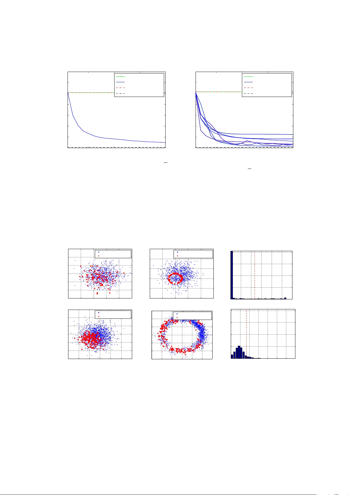
A daptiv e sequen tial Mon te Carlo b y means of mixture of exp erts Julien Cornebise ∗ E. Moulines † , J. Olsson ‡ Septem b er 13th th , 2012 Abstract: Appropriately designing the prop osal k ernel of particle ﬁlters is an issue of signiﬁcan t importance, since a bad choice ma y lead to deterioration of the particle sam- ple and, consequen tly , w aste of computational p o w er. In this pap er w e introduce a nov el algorithm adaptiv ely approximating the so- called optimal proposal k ernel by a mixture of in tegrated curved exponential distributions with logistic w eights. This family of distri- butions, referred to as mixtur es of exp erts , is broad enough to be used in the presence of m ulti-mo dalit y or strongly skew ed distribu- tions. The mixtures are ﬁtted, via online-EM metho ds, to the optimal kernel through min- imisation of the Kullback-Leibler divergence b et w een the auxiliary target and instrumen- tal distributions of the particle ﬁlter. A t eac h iteration of the particle ﬁlter, the algorithm is required to solv e only a single optimisation problem for the whole particle sample, yield- ing an algorithm with only linear complexity . In addition, w e illustrate in a simulation study ho w the metho d can b e successfully applied to optimal ﬁltering in nonlinear state-space mo d- els. Keyw ords: Optimal prop osal k ernel, A daptive algorithms, Kullback-Leibler diver- gence, Co eﬃcien t of v ariation, Expectation- maximisation, P article ﬁlter, Sequen tial Mon te Carlo, Shannon entrop y 1 In tro duction During the last decade, sequential Mon te Carlo (SMC) methods hav e dev elop ed from b eing a to ol for solving sp eciﬁc problems, such as the optimal ﬁltering problem in general state-space models or simulation of rare even ts (these topics are abundantly cov ered in Liu, 2001; Doucet et al., 2001; Ristic et al., 2004; Capp é et al., 2005; Del Moral et al., 2006, and the references therein). The high ﬂexi- bilit y of these methods mak es it p ossible to use them for eﬃciently executing key steps of comp osite algorithms tac kling very complex problems, e.g., as in particle Mark ov chain Mon te Carlo (MCMC) methods for join t in- ference on static and dynamic v ariables (se e Andrieu et al., 2010). Ho wev er, while there has been abundan t w ork on adaptation of MCMC metho ds, from the early algorithms of Haario et al. (2001) to the mathematical study of disminishing adap- tation established in Andrieu and Moulines (2006) and Rob erts and Rosenthal (2009), adaptiv e metho ds for SMC are still in their in- fancy . This article, which sets out from a theo- retical framework for adaptiv e SMC presen ted in Cornebise et al. (2008), is part of the eﬀort to ﬁll this gap—which is required to achiev e maxim um eﬃciency and user-friendliness. A mathematically less detailed pre-version of the presen t pap er appeared as part of the Ph. D. dissertation by Cornebise (2009). Suc h adaptiv e methods are esp ecially suited to cop e with the rising complexit y of state-sp ac e mo dels (SSMs) in recen t applica- tions. While simple unidimensional ﬁltering problems will rarely justify ev en a sligh t com- putational ov erhead of adaptiv e metho ds ov er plain SMC metho ds (such as the b o otstr ap p ar- ticle ﬁlter ; see Section 3.1), the situation is re- v ersed for man y state-of-the-art SSMs, where forw ard simulation may require costly ph ys- ical emulators or the ev aluation of computa- tionally exp ensiv e transition densities. This o ccurs, e.g., as so on as the mo del in volv es dif- feren tial equations and numeric solutions of ∗ julien@cornebise.com † Département T raitement du Signal et de l’Image, T elecom ParisT ech ‡ Centre for Mathematical Sciences, Lund Universit y 1 the same. Recen t examples range from health sciences (see e.g. Korotsil et al., 2012, for a study of the epidemiology of human papillo- ma virus infections) to environmen tal sciences (see e.g. Robins et al., 2009, who studied data assimilation for atmospheric disp ersion of hazardous airb orne biological material). In the SMC framew ork, the ob jectiv e is to approximate a se quenc e of target densities, deﬁned on a sequence of state spaces as fol- lo ws. Giv en a density µ on some state space Ξ , the next densit y ˜ µ in the sequence is de- ﬁned by ˜ µ ( ˜ x ) := R µ ( x ) l ( x , ˜ x ) d x R R µ ( x ) l ( x , ˜ x ) d x d ˜ x , ˜ x ∈ ˜ Ξ , (1.1) where ˜ Ξ is some other state space and l : Ξ × ˜ Ξ → R + is an un-normalised transition densit y . Here the dimensions of ˜ Ξ and Ξ t yp- ically diﬀer. This framework encompasses, in- ter alia, the classical problem of optimal ﬁl- tering in SSMs recalled in Section 6 (see in particular Equation (6.4)). SMC metho ds approximate online the den- sities generated by (1.1) by a recursiv ely up- dated set of random p articles { X i } N i =1 and as- so ciated imp ortanc e weights { ω i } N i =1 . A t each iteration of the algorithm, the weigh ted par- ticle sample { ( X i , ω i ) } N i =1 appro ximates the corresp onding target densit y µ in the sense that P N i =1 ω i f ( X i ) / Ω , with Ω := P N ` =1 ω ` , appro ximates E µ [ f ( X )] := R f ( x ) µ ( x ) d x (this will b e our generic notation for expecta- tions) for all b ounded measurable functions f on the corresponding state space Ξ . All SMC metho ds ha v e tw o main operations in com- mon: a mutation step and a sele ction step . In the former, the particles are randomly scat- tered in the state space by means of a pr o- p osal transition density r : Ξ × ˜ Ξ → R + ; more sp eciﬁcally , the m utation op eration gen- erates a set of new, ˜ Ξ -v alued particles b y mov- ing the particles according to the transition densit y r and assigning each mutated particle an up dated imp ortance weigh t prop ortional to l/r ; consequently , each w eight reﬂects the rel- ev ance of the corresp onding particle as mea- sured by the lik eliho o d ratio. In general, the m utated particles are conditionally indep en- den t given the ancestor particles. In the selec- tion step, the particles are duplicated or elimi- nated with probabilities depending on the im- p ortance w eights. This is t ypically done by m ultinomially resampling the particles with probabilities prop ortional to the corresp ond- ing weigh ts. In the auxiliary p article ﬁlter (prop osed b y Pitt and Shephard, 1999) the particles are resampled according to weigh ts that are mo diﬁed b y a factor determined by an adjustment multiplier function a : Ξ → R + . In tro ducing adjustmen t m ultipliers mak es it p ossible to, by using some conv enien t look a- head strategy , increase the w eight of those particles that will most likely contribute sig- niﬁcan tly to the approximation of the subse- quen t target distribution after having b een se- lected. In this wa y computational pow er is di- rected tow ard zones of the state space where the mass of the subsequent target density is lo cated. The choice of the adjustmen t w eight func- tion a and the prop osal densit y r aﬀects sig- niﬁcan tly the qualit y of the generated sam- ple, and in this pap er we focus on adap- tiv e design of the latter. Letting r ( x , ˜ x ) = l ( x , ˜ x ) / R l ( x , ˜ x ) d ˜ x is app ealing as the parti- cles in this case are propagated according to a dynamics that is closely related to that of the recursion (1.1). Indeed, by com bining this c hoice of prop osal kernel w ith the adjustment m ultiplier function a ( x ) = R l ( x , ˜ x ) d ˜ x yields p erfectly uniform imp ortance w eights. In this case the SMC algorithm is referred to as ful ly adapte d . How ever, this so-called optimal pro- p osal kernel and adjustment multiplier weigh t function can b e expressed on closed-form only in a few cases and one is in general referred to appro ximations of these quantities. There is a large literature dealing with the problem of approximating the optimal pro- p osal k ernel. When using SMC for optimal ﬁltering in SSMs, Doucet et al. (2000) sug- gest approximating each function l ( x , · ) by a Gaussian density whose mean and cov ariance are obtained using the extende d Kalman ﬁlter . A similar approac h based on the unsc ente d Kalman ﬁlter was prop osed by V an der Merwe et al. (2000) (see also V an der Merw e and W an, 2003). This tec hnique presupp oses that the mo del under consideration can b e w ell appro ximated b y a nonlinear Gaussian SSM with linear measuremen t equation; how ever, this far from alwa ys the case, and careless lin- earisation (e.g. in cases where the lo cal like- liho od is multimodal) ma y b oomerang and cause severe deterioration of the particle sam- ple. Cappé et al. (2005, Section 7.2.2.4) make a form of Laplace approximation of l ( x , · ) b y simply lo cating the mo de of the function in question and centering a Gaussian density or the density of a student’s t -distribution around the same. This technique, which go es bac k to Pitt and Shephard (1999), is appro- 2 priate when the function is log-concav e (or strongly unimo dal); nevertheless, as the mo de of eac h l ( x , · ) is a function of x , this approach in volv es solving one optimisation problem per particle. Thus, in spite of this in tense re- cen t activit y in the ﬁeld, the state-of-the-art algorithms ha ve met only mitigated success as they implicitly assume that the functions l ( x , · ) hav e a single mo de. A common practice (see e.g. Oh and Berger, 1993) for designing prop osal distri- butions in standard (non-sequen tial) imp or- tance sampling is to consider a parametric family of prop osal distributions and then iden- tify a parameter that minimizes some mea- sure of discrepancy b etw een the target and the prop osal distributions. Common c hoices are the widely used squared c o eﬃcient of varia- tion of the imp ortance weigh ts or the negated Shannon entr opy (see e.g. Capp é et al., 2005, p. 235, for deﬁnitions of these quantities) of the same. Both are maximal when the sample is completely degenerated, i.e. when one sin- gle particle carries all the weigh t, and minimal when all the importance weigh ts are equal. The co eﬃcien t of v ariation often appears in a transformed form as the eﬀe ctive sample size (w e refer again to Cappé et al., 2005, for a deﬁnition). The same quan tities ha ve b een widely used also within the framew ork of SMC, but un til recen tly only for trigger- ing selection and not as a tool for adaptive design of the instrumen tal distribution. The k ey result of Cornebise et al. (2008, Theorems 1 and 2) was to relate the Shannon en tropy to the Kul lb ack-L eibler diver genc e (KLD; see Equation (3.6)) b et ween the instrumen tal and prop osal distributions of the particle ﬁlter. More sp eciﬁcally , when selection is carried through using multinomial resampling, eac h particle cloud up date (selection follo wed b y resampling) can b e viewed as standard impor- tance sampling where a w eighted mixture of N stratas—the i th stratum being prop ortional to ω i l ( X i , · ) —appro ximating ˜ µ is targeted us- ing a mixture prop osal π comprising N stratas prop ortional to { ω i r ( X i , · ) } N i =1 . As the n um- b er of particles tends to inﬁnit y , one may pro ve that the KLD betw een these tw o mix- tures tends to the KLD b et ween tw o distribu- tions ha ving densities µ ∗ ( x , ˜ x ) ∝ l ( x , ˜ x ) µ ( x ) and π ∗ ( x , ˜ x ) ∝ a ( x ) r ( x , ˜ x ) µ ( x ) , which can b e view ed as “asymptotic” target and prop osal distributions on the product space Ξ × ˜ Ξ . In addition, one may pro ve that the Shan- non en tropy has the same limit. (Cornebise et al. (2008) established a similar relation be- t ween the co eﬃcient of v ariation of the parti- cle w eights and the chi-squar e diver genc e be- t ween the same distributions.) This gives a sound theoretical supp ort for using the Shan- non entrop y of the importance weigh ts for measuring the quality of the particle sample. In addition, it suggests that the KLD b et ween the target mixture and π could b e used in lieu of the Shannon entrop y for all purposes, es- p ecially adaptation. As a matter of fact, in the context of adaptive design of SMC meth- o ds, the KLD is (as p oin ted out by Cornebise et al., 2008, Section 2.3) highly practical since it decouples the adaptation of the adjustmen t w eight function a and that of the prop osal ker- nel r ; see the next section. Henceforth, in the present article we ex- tend and implement fully the metho dology indicated and sketc hed by Cornebise et al. (2008) and select the auxiliary prop osal dis- tribution π from a family { π θ ; θ ∈ Θ } of can- didate distributions b y picking θ ∗ suc h that the KLD b et ween the target mixture and π θ ∗ is minimal and letting π = π θ ∗ . On the one hand, the c hosen parametric family should b e ﬂexible enough to approximate complex transition k ernels; on the other hand, sam- pling from π θ should b e easy . Finally , the pa- rameterisation should b e done in such a wa y that the problem of estimating the param- eters is as simple as possible. In this arti- cle, w e suggest mo deling the prop osal π θ as a mixture of in tegrated curved exp onen tial dis- tributions. By letting the mixture weigh ts of the c hosen prop osal dep end on the an- cestor particles { X i } N i =1 , w e allow for parti- tioning of the input space into regions corre- sp onding to a sp ecialised kernel. Each com- p onen t of the mixture b elongs to a family of integrated curved exp onen tial distributions, whose tw o most known mem b ers are the m ul- tiv ariate Gaussian distribution and the Stu- den t’s t -distribution. Also the parameters of the mixture dep end on the ancestors { X i } N i =1 . This parameterisation of the prop osal distri- bution is closely related to the (hierarchical) mixtur e of exp erts app earing in the machine learning communit y and describ ed in (Jor- dan and Jacobs, 1994; Jordan and Xu, 1995). The ﬂexibility of our approach allows for ef- ﬁcien t approximation of the optimal kernel for a large class of intricate (nonlinear non- Gaussian) mo dels. Unlik e t ypical EM-t yp e parameter estimation procedures, whic h are in general run iterativ ely un til stabilisation, our adaptive SMC algorithm only requires a decrease of the KLD, not an exact minimum. 3 As illustrated in our examples in Section 6, suc h a gain typically o ccurs already at early iterations of the algorithm (a characteristic of EM-t yp e algorithms), impliying the need of only v ery few EM iterations and therefore a minimal computational ov erhead. The pap er is organized as follows. In the next section we in tro duce some matrix nota- tion and list the most common notation used throughout the pap er. Section 3 describ es, in a nutshell, auxiliary SMC methods as well as a KLD-based approach to adaptation of these methods that is used in the pap er. Sec- tion 4 recalls mixtures of exp erts and Section 5 treats optimisation of the mixture parameters b y means of stochastic approximation meth- o ds; the latter section is the core of the pap er and contains our main results. In Section 6 we illustrate the eﬃciency of the metho d on sev- eral simulation-based examples and Section A con tains some pro ofs. 2 Notation 2.1 Matrix notation All vectors and matrices are typeset in b old- face. V ectors are c olumn ve ctors unless pre- cised diﬀeren tly . The i th column vector of a matrix A is denoted b y A | i . W e denote by T r( A ) the trace of a matrix A and for an y matrices A and B of dimensions m × n and p × q , respectively , w e denote their dir e ct sum b y A  B :=  A 0 p × q 0 m × n B  , (2.1) whic h is such that ( A  B ) | = A |  B | and, for any tw o matrices C and D of compatible dimensions, ( A  B )( C  D ) | = ( A C | )  ( BD | ) , where | denotes the transp ose. 2.2 List of notation The following quantities are deﬁned in the corresp onding equations. Quan tity Equation a ∗ (3.3) α j (4.5) d KL (3.6) η (4.2) φ k (6.3) G (6.2) g (6.2) Quan tity Equation h (5.15) κ (5.23) l (5.8) l ∗ (3.2) ˜ µ (1.1) ¯ p (5.7) ˜ p (5.21) π θ (4.3) ¯ π θ ( ) (5.1) ¯ π θ ( | ) (5.5) r θ (4.1)  (2.1) Q (6.1) q (6.1) ρ (4.1) ¯ ρ ( ) (4.6) ¯ ρ ( | ) (5.2) ¯ s (5.6) ˜ s (5.20) ¯ t (5.27) ˜ t (5.28) θ (4.2) ¯ θ (5.9) ¯ v (5.27) ˜ v (5.28) w θ (4.4) 3 Preliminaries 3.1 Auxiliary SMC metho ds In order to precisely describe one iteration of the SMC algorithm, let µ be a target prob- abilit y densit y function o ver a space Ξ and supp ose that we hav e at hand a weigh ted sam- ple { ( X i , ω i ) } N i =1 suc h that P N i =1 ω i f ( X i ) / Ω , with Ω = P N i =1 ω i , estimates R f ( x ) µ ( x ) d x for any µ -in tegrable function f . As a nota- tional conv ention, we use capitals to denote random v ariables and low er case for function argumen ts. W e now wish to transform (by moving the particles and adjusting accordingly the imp or- tance weigh ts) the sample { ( X i , ω i ) } N i =1 in to a new w eighted particle sample approximat- ing the probability density ˜ µ deﬁned on ˜ Ξ through (1.1). Ha ving access to { ( X i , ω i ) } N i =1 , an approximation of ˜ µ is naturally obtained b y plugging the weigh ted empirical measure as- so ciated with this weigh ted sample in to (1.1), 4 yielding the mixture density ˜ µ ( ˜ x ) ≈ P N i =1 ω i l ( X i , ˜ x ) P N j =1 ω j R l ( X j , ˜ x ) d ˜ x = N X i =1 ω i a ∗ ( X i ) P N j =1 ω j a ∗ ( X j ) l ∗ ( X i , ˜ x ) ! , (3.1) where we hav e in tro duced the normalised transition density l ∗ ( x , ˜ x ) := l ( x , ˜ x ) R l ( x , ˜ x ) d ˜ x (3.2) and the partition function a ∗ ( x ) := Z l ( x , ˜ x ) d ˜ x (3.3) of l ( x , · ) , and ideally an up dated particle sam- ple would b e obtained by drawing new parti- cles { ˜ X i } N i =1 indep enden tly from (3.1). There are how ever tw o problems with this approach: ﬁrstly , in general, the integral R l ( · , ˜ x ) d ˜ x lacks closed-form expression, ruling out direct com- putation of the mixture w eights; secondly , ev en if the integral was known in closed form, the resulting algorithm would hav e an O ( N 2 ) computational complexity due to the normal- ization of the mixture w eights. T o cop e with these issues, w e will, as prop osed by Pitt and Shephard (1999), aim instead at sampling from an auxiliary tar get distribution having densit y ¯ µ ( i, ˜ x ) := ω i a ∗ ( X i ) P N j =1 ω j a ∗ ( X j ) l ∗ ( X i , ˜ x ) , (3.4) o ver the pro duct space { 1 , . . . , N } × ˜ Ξ of indices and particle p ositions. T o sam- ple ¯ µ w e take an imp ortance sampling ap- proac h consisting in drawing independent pairs { ( I i , ˜ X i ) } N i =1 of indices and p ositions from the prop osal distribution π ( i, ˜ x ) := ω i a ( X i ) P N j =1 ω j a ( X j ) r ( X i , ˜ x ) (3.5) o ver the same extended space and assign- ing each draw ( I i , ˜ X i ) the imp ortance weigh t ˜ ω i := w ( I i , ˜ X i ) , where w ( i, ˜ x ) := l ( X i , ˜ x ) a ( X i ) r ( X i , ˜ x ) ∝ ¯ µ ( i, ˜ x ) π ( i, ˜ x ) . Here r and a are the proposal transition den- sit y resp. adjustment m ultiplier weigh t func- tion men tioned in the in troduction. As for all importance sampling, it is crucial that the target distribution ¯ µ is absolutely con tinuous with respect to the proposal distribution π . W e th us require that the adjustment multi- plier weigh t function is p ositiv e and that the prop osal transition densit y is such that for all x ∈ Ξ , r ( x , ˜ x ) = 0 ⇒ l ( x , ˜ x ) = 0 , i.e. the supp ort of l ( x , ˜ x ) in included in that of r ( x , ˜ x ) . Finally , we discard the indices I i and k eep { ( ˜ X i , ˜ ω i ) } N i =1 as an approximation of ˜ µ . This sc heme, which is traditionally re- ferred to as the auxiliary particle ﬁlter (Pitt and Shephard, 1999), encompasses the sim- pler framework of the b ootstrap particle ﬁlter prop osed originally b y Gordon et al. (1993), whic h simply amounts to setting a = 1 Ξ (im- plying a gain of simplicit y at the price of ﬂex- ibilit y). Moreo ver, SMC sc hemes where re- sampling is p erformed only at random times can similarly b e cast in to the setting of the auxiliary particle ﬁlter b y comp osing the ker- nels in v olved in several consecutive steps of the of recursion (1.1) (see e.g. Cornebise, 2009, Chapter 4, for details). A theoretical analy- sis of b ootstrap-type SMC metho ds with ran- dom resampling sc hedule is also given by Del Moral et al. (2012). Therefore, any metho d- ology built for the auxiliary particle ﬁlter also applies to these simpler framew orks without mo diﬁcation. 3.2 A foundation of SMC adap- tation W e now describ e a foundation of SMC adapta- tion underpinning the coming dev elopments. Recall that the KLD betw een t wo distribu- tions µ and ν , deﬁned on the same state space Ξ , is deﬁned as d KL ( µ k ν ) := E µ  log dµ dν ( X )  , (3.6) pro vided that µ is absolutely con tinuous with resp ect to ν . Here E µ denotes the exp ectation under µ . Casting the KLD in to the frame- w ork of SMC metho ds and replacing µ and ν b y the auxiliary target distribution ¯ µ and the prop osal π , resp ectiv ely , yields d KL ( ¯ µ k π ) = E ¯ µ " log ¯ µ ( I , ˜ X ) π ( I , ˜ X ) # , (3.7) 5 whic h decouples as d KL ( ¯ µ k π ) = E ¯ µ " log l ∗ ( X I , ˜ X ) r ( X I , ˜ X ) # | {z } Dep ends only on r + E ¯ µ " log ω I a ∗ ( X I ) / P N j =1 ω j a ∗ ( X j ) ω I a ( X I ) / P N j =1 ω j a ( X j ) # | {z } Dep ends only on a . (3.8) As clear from the deﬁnition (3.4), the mea- sure ¯ µ is random as it dep ends on the ances- tor particles { X i } N i =1 ; the lo cations of the lat- ter should thus be viewed as ﬁxed within the brac kets of the exp ectations in (3.7) and (3.8). The ﬁrst term in (3.8) corresp onds to the dis- crepancy induced b y mutating the particles { ˜ X i } N i =1 using a suboptimal proposal k ernel, and the second term corresponds to the dis- crepancy induced by sampling the ancestor in- dices { I i } N i =1 according to sub optimal adjust- men t weigh ts. Moreov er, d KL ( ¯ µ k π ) = − E ¯ µ h log r ( X I , ˜ X ) i − E ¯ µ " log a ( X I ) P N j =1 ω j a ( X j ) # + c where the additiv e term c in volv es the opti- mal quantities a ∗ and l ∗ only and is irrelev an t for the optimisation problem. Equalit y up to a constant will in the follo wing b e denoted b y ≡ . R estricting ourselves to adaptation of the pr op osal kernel , we obtain the simple expres- sion d KL ( ¯ µ k π ) ≡ − E ¯ µ h log r ( X I , ˜ X ) i . (3.9) In the next section we presen t a method for minimising the KLD (3.9) ov er a fam- ily { π θ ; θ ∈ Θ } of instrumental distributions where the prop osal transition density of eac h mem b er belongs to parametrised family of mixtures of exp erts. F ormally , we will solv e θ ∗ := arg min θ ∈ Θ d KL ( ¯ µ k π θ ) (3.10) and take π = π θ ∗ . Although the right hand side of (3.9) is most often not directly com- putable, such a quantit y can b e appro ximated on-the-ﬂy using the weigh ted sample already generated; the resulting algorithms (Algo- rithms 1 and 2; see Section 5) closely resem- bles the cr oss-entr opy metho d (see Rubinstein and Kro ese, 2004) method. 4 Mixture of exp erts In this contribution, we consider Ξ = R p and ˜ Ξ = R ˜ p and let the prop osal k ernel hav e den- sit y (with resp ect to Leb esgue measure) r θ ( x , ˜ x ) := d X j =1 α j ( x ; β ) ρ ( x , ˜ x ; η j ) , (4.1) where { α j } d j =1 are nonnegativ e weighting functions summing in to unity and ρ is a Mark ov transition k ernel from Ξ to ˜ Ξ . The w eighting functions and the Mark ov transi- tion densit y are parametrised b y parameters β and η , resp ectiv ely , and the j th stratum of the mixture is characterised b y a certain c hoice η j of the latter. The integer d is ﬁxed. Denote η := { η 1 , . . . , η d } , θ :=  β , η  . (4.2) Putting (4.1) into the auxiliary particle ﬁlter framew ork in Section 3.1, the asso ciated pro- p osal distribution is giv en by π θ ( i, ˜ x ) = ω i a ( X i ) P N ` =1 ω ` a ( X ` ) d X j =1 α j ( X i , β ) ρ ( X i , ˜ x ; η j ) . (4.3) W e then assign the imp ortance w eight ˜ ω i = w θ ( I i , ˜ X i ) to eac h dra w ( I i , ˜ X i ) from π θ , where w θ ( i, ˜ x ) = l ( X i , ˜ x ) a ( X i ) P d j =1 α j ( X i , β ) ρ ( X i , ˜ x ; η j ) ∝ ¯ µ ( i, ˜ x ) π θ ( i, ˜ x ) . (4.4) The set { α j } d j =1 of weigh t functions typically partitions the input space Ξ in to sub-regions with smo oth transitions b y assigning a v ec- tor of mixture w eights to eac h point of the input space. In each sub-region, one pro- p osal kernel will ev entually dominate the mix- ture, sp ecialising the whole prop osal r θ on a p er-region basis. As in Jordan and Xu (1995), we consider lo gistic w eight functions, i.e. β = { β 1 , . . . , β d − 1 } and α j ( x , β ) :=        exp( β | j x ) 1 + P d − 1 ` =1 exp( β | ` x ) , j 6 = d, 1 1 + P d − 1 ` =1 exp( β | ` x ) , j = d, (4.5) 6 where x := ( x | 1) | and the β j ’s are vectors in R p +1 . It is sometimes of interest to resort to simpler mixtures whose weigh ts do not dep end on x b y letting, for a set β = ( β j ) d j =1 nonneg- ativ e scalars summing into unity , α j ( x , β ) := β j , 1 ≤ j ≤ d , indep enden tly of x and hence without partitioning the input space. This mo del for the transition kernel is the n simi- lar to the switching r e gr ession mo del (Quandt and Ramsey, 1972). The original mixture of exp erts prop osed b y Jordan and Jacobs (1994) was based on Gaussian strata ρ , which is indeed is the most straigh tforward choice. How ev er the same al- gorithm can, at no additional cost, b e ex- tended to the broader class of densities of in- te gr ate d curve d exp onential form , describ ed in Assumption 4.1 below, whic h still allo ws for the same trade-oﬀ betw een ﬂexibility , ease of sampling, and conv enien t estimation. Assumption 4.1 Ther e exist a state sp ac e Υ ⊆ R u and a Markov tr ansition kernel fr om Ξ to ˜ Ξ × Υ having a density of form ¯ ρ ( x , ( ˜ x , u ); η ) := γ ( u ) h ( x , ˜ x , u ) × exp ( − a ( η ) + T r( b ( η ) | s ( x , ˜ x , u ))) , (4.6) wher e the functions γ , h , a and s , b ar e r e al- value d r esp. R s × s 0 -value d, such that ρ ( x , ˜ x ; η ) = Z Υ ¯ ρ ( x , ( ˜ x , u ); η ) d u . (4.7) In other words, ρ ( x , ˜ x ; η ) is the densit y of the marginal of a curved exp onential distribution. In (4.6), s is a vector of suﬃcien t statistics. In the next section we presen t a method ﬁtting eﬃciently the prop osal π θ to the target ¯ µ b y solving (3.10). W e will illustrate the de- tails for the sp eciﬁc case of m ultidimensional Gaussian distributions and multidimensional studen t’s t -distributions. It should ho wev er b e kept in mind that the algorithm is v alid for an y member of the family of integrated curved exp onen tial distributions as long as Assump- tion 5.1 b elo w is fulﬁlled. 5 Main results and algo- rithms In the following we discuss how the intricate optimisation problem (3.10) can b e cast into the framework of latent data pr oblems . Pa- rameter estimation for mixtures of exp erts is most often carried through using the EM al- gorithm (see McLachlan and Krishnan, 2008, Section 8.4.6), and also in this paper a re- cursiv e EM-type algorithm will b e used for ﬁnding close to optimal mixture parameters. More precisely , we dev elop an algorithm that is closely related to the online EM algorithm for latent data mo dels prop osed b y Cappé and Moulines (2009). F rom a practical point of view, a k ey feature of the adaptive SMC ap- proac h describ ed in Section 3.2 is that it aims at decreasing the KLD rather than obtaining a fully conv erged parameter estimate: v ery few EM iterations are therefore needed for obtain- ing a signiﬁcant computational gain. This will b e illustrated further in the simulation study of Section 6. 5.1 Main assumptions and deﬁ- nitions In order to describ e clearly the algorithm, we limit ourselves initial ly to the c ase of c onstant mixtur e weights , i.e. we let α j ( x , β ) := β j , 1 ≤ j ≤ d , for a set β = { β j } d j =1 of nonneg- ativ e scalars summing into unity . The more general c hoice (4.5) will b e treated in Sec- tion 5.3. W e no w augmen t the pair ( I , ˜ X ) with the index J of the mixture comp onent as w ell as the auxiliary , Υ -v alued v ariable U of the curved exp onen tial family . More sp eciﬁ- cally , w e in tro duce an extended random v ari- able ( I , J, ˜ X , U ) having mixed-type distribu- tion with probability function ¯ π θ ( i, j, ˜ x , u ) := ω i a ( X i ) P N ` =1 ω ` a ( X ` ) α j ( X i , β ) ¯ ρ ( X i , ( ˜ x , u ); η j ) (5.1) on the pro duct space { 1 , . . . , N } × { 1 , . . . , d } × ˜ Ξ × Υ . It is easily c hec ked that π θ is the marginal of ¯ π θ in I and ˜ X . The following assumption is critical for con venien t estima- tion. Although surprising at ﬁrst glance, it simply requires that the state space extension used for handling integrated curved exponen- tial distributions can b e easily rev erted for the suﬃcien t statistics: the exp ectation of the suf- ﬁcien t statistics under the conditional distri- bution of U giv en X I = x and ˜ X = ˜ x , having densit y ¯ ρ ( u | x , ˜ x ; η ) := ¯ ρ ( x , ( ˜ x , u ); η ) ρ ( x , ˜ x ; η ) , (5.2) should b e a v ailable in closed form. Since the suﬃcien t statistics of exp onen tial families of- ten hav e a simple form, this assumption is 7 most often satisﬁed; e.g. it is satisﬁed for the Studen t’s t -distribution in Example 5.2. Assumption 5.1 F or al l η and ( x , ˜ x ) ∈ Ξ × ˜ Ξ , the exp e ctation Z s ( x , ˜ x , u ) ¯ ρ ( u | x , ˜ x ; η ) d u (5.3) is available in close d form. Under Assumption 5.1, let for j ∈ { 1 , . . . , d } , ¯ p j ( θ ) := E ¯ µ h ¯ π θ ( j | I , ˜ X ) i , ¯ s j ( θ ) := E ¯ µ  ¯ π θ ( j | I , ˜ X ) × Z s ( X I , ˜ X , u ) ¯ ρ ( u | X I , ˜ X ; η j ) d u  , (5.4) where we hav e deﬁned the r esp onsibilities ¯ π θ ( j | i, ˜ x ) := R ¯ π θ ( i, j, ˜ x , u ) d u P d ` =1 R ¯ π θ ( i, , ˜ x , u ) d u = β j ρ ( X i , ˜ x ; η j ) P d ` =1 β ` ρ ( X i , ˜ x ; η ` ) . (5.5) Note that the quan tities deﬁned in (5.4) de- p end implicitly on the ancestor sample. In addition, we collect these statistics in the ma- trix ¯ s ( θ ) := ¯ s 1 ( θ )  ¯ s 2 ( θ )  · · ·  ¯ s d ( θ ) (5.6) and the vector ¯ p ( θ ) := ( ¯ p 1 ( θ ) , ¯ p 2 ( θ ) , . . . , ¯ p d ( θ )) | . (5.7) W e imp ose the follo wing additional as- sumption. Assumption 5.2 Ther e ar e subsets Π ⊆ R d + and Σ ⊆ R s × s 0 such that for al l { s j } d j =1 ∈ Σ d and p ∈ Π , the mapping θ 7→ l ( s , p ; θ ) := − ( a ( η 1 ) , . . . , a ( η d )) p + (log β 1 , . . . , log β d ) p + d X j =1 T r( b ( η j ) | s j ) (5.8) has unique glob al maximum denote d by ¯ θ ( s , p ) . In p articular, ¯ θ ( s , p ) := arg max θ ∈ Θ l ( s , p ; θ ) . (5.9) Remark 5.1 (De c oupling, optimal str ata weights) It should b e note d that due to the additive form of l , the optimisation pr ob- lem (5.9) c an b e split into the two sep ar ate subpr oblems 1. ( arg max β (log β 1 , . . . , log β d ) p subje ct to P d j =1 β j = 1 2. arg max η   ( a ( η 1 ) , . . . , a ( η d )) p + d X j =1 T r  b ( η j ) | s j    , c orr esp onding to maximisation over mixtur e weights and str ata p ar ameters, r esp e ctively. In the fr amework c onsider e d so far, wher e the mixtur e weights ar e assume d to b e c onstant, the ﬁrst of these pr oblems (1) has, for al l p ∈ R d + the solution ¯ β j = p j P d ` =1 p ` for al l j . In the following t wo examples w e specify the solution to the second problem (2) in Re- mark 5.1 for the tw o—fundamental—special cases of multivariate Gaussian distributions and multivariate Student’s t -distributions ; it should how ever b e k ept in mind that the metho d is v alid for an y in tegrated curved exp onen tial distribution satisfying Assump- tion 5.1. Example 5.1 (Up dating formulas for Gaussian str ata) In a ﬁrst example we let e ach str atum b e the density of a line ar Gaus- sian r e gr ession p ar ameterise d by η = ( µ , Σ ) . The original hier ar chic al mixtur e of exp erts was b ase d on plain Gaussian distributions and a p ossibly de ep hier ar chy of exp erts, incurring a c omputational overhe ad p ossibly lar ger than aﬀor dable for an algorithm use d for adapti- ation. Dr opping the hier ar chic al appr o ach is a p ossible way to r e duc e this overhe ad at the pric e of r e duc e d ﬂexibility. Her e we c om- p ensate somewhat for this loss by using a line ar r e gr ession within e ach exp ert. Thus, given J = j , the new p article lo c ation ˜ X has p 0 -dimensional Gaussian distribution with me an µ j X I , wher e the regression matrix µ j is of size p 0 × ( p + 1) , and symmetric, p os- itive deﬁnite co v ariance matrix Σ j of size 8 p 0 × p 0 . In this c ase, the suﬃcient statistics ar e s ( x , ˜ x , u ) = ( ˜ x ˜ x | )  ( xx | )  ( ˜ x x | ) , le ad- ing to the exp e cte d r esp onsibilities ¯ p j ( θ ) := E ¯ µ h ¯ π θ ( j | I , ˜ X ) i and the exp e cte d suﬃcient statistics ¯ s j ( θ ) := ¯ s j, 1 ( θ )  ¯ s j, 2 ( θ )  ¯ s j, 3 ( θ ) with ¯ s j, 1 ( θ ) := E ¯ µ h ¯ π θ ( j | I , ˜ X ) ˜ X ˜ X | i , ¯ s j, 2 ( θ ) := E ¯ µ h ¯ π θ ( j | I , ˜ X ) X I X | I i , ¯ s j, 3 ( θ ) := E ¯ µ h ¯ π θ ( j | I , ˜ X ) ˜ X X | I i . In addition, the functions a and b in (4.6) ar e in this c ase given by a ( η ) = 1 2 log | Σ | , b ( η ) =  − 1 2 Σ − 1    − 1 2 µ Σ − 1 µ |    − Σ − 1 µ  . (5.10) Conse quently, the ar gument η j that maxi- mizes l ( s , p ; θ ) for a given suﬃcient statistics s j is given by ¯ µ j ( s j ) := s j, 3 s − 1 j, 2 , ¯ Σ j ( p j , s j ) := p − 1 j  s j, 1 − s j, 3 s − 1 j, 2 s | j, 3  . R emark 5.2 (Po oling the c ovarianc es) In pr actic e, a r obustiﬁe d version of the algo- rithm ab ove c an b e obtaine d by p ooli ng the c o- varianc es (se e e.g. R ayens and Gr e ene, 1991). This me ans that a c ommon c ovarianc e matrix is use d for al l the c omp onents of the mixtur e, i.e. Σ j = Σ for al l j . By doing this, the wel l- known pr oblem of mixtur e mo dels with str ata c omp onents de gener ating to Dir ac masses is avoide d. It is str aightforwar d to enfor c e such a r estriction in the optimisation pr o c e dur e ab ove, le ading to ¯ Σ j ( p j , s j ) := d − 1 d X ` =1  s `, 1 − s `, 3 s − 1 `, 2 s | `, 3  (5.11) for al l j . Example 5.2 (Up dating formulas for Student’s t -distribution-b ase d str ata) A c ommon grip in imp ortanc e sampling (se e, for instanc e, Oh and Ber ger, 1993) is to r eplac e, in or der to al low for mor e eﬃcient ex- plor ation of the state sp ac e, Gaussian distribu- tions by Student’s t -distributions. Ther efor e, as a mor e r obust alternative to the appr o ach taken in Example 5.1, one may use inste ad a p 0 -dimensional Student’s t -distribution with ν de gr e es of fr e e dom, i.e. ρ ( x , ˜ x ; η j ) = t p 0 ( ˜ x ; µ j x , Σ j , ν ) . (5.12) R emark 5.3 (Fixing the de gr e es of fr e e- dom) The numb er ν of de gr e es of fr e e dom of the Student’s t -distributions is ﬁxe d, typic al ly to ν ∈ { 3 , 4 } , b efor ehand and is c ommon to al l str ata. A similar choic e has b e en made by, among others, Pe el and McL achlan (2000, Se ction 7) and Capp é et al. (2008) as it al lows for close d form optimisation in the M -step. The choic e (5.12) c an b e c ast into the fr ame- work of Se ction 4, with Υ = R , thanks to the Gaussian - Gamma decomp osition of mul- tivariate Student’s t -distributions use d by Liu and Rubin (1995, Se ction 2) and Pe el and McL achlan (2000, Se ction 3): t ( ˜ x ; µ x , Σ , ν ) = Z ∞ 0 N  ˜ x ; µ x , Σ u − 1  γ  u ; ν 2 , ν 2  du, wher e γ ( u ; a, b ) := b a u a − 1 exp( − bu ) / Γ( a ) is the density of the Gamma distribution with shap e p ar ameter a and sc ale p ar am- eter b . Henc e, the multivariate Student’s t -distribution is an inte gr ate d curve d ex- p onential distribution (4.6) with γ ( u ) = γ ( u ; ν / 2 , ν / 2) , h ( x , ˜ x , u ) = (2 π ) − p/ 2 , suﬃ- cient statistics s ( x , ˜ x , u ) = ( u ˜ x ˜ x | )  ( u xx | )  ( u ˜ xx | ) , and the same a and b as in the Gaussian c ase (5.10) . Sinc e the Gamma dis- tribution is c onjugate prior with r esp e ct to pr e cision for the Gaussian distribution with known me an, the exp e ctation η of U under ¯ ρ ( u | x , ˜ x ; η ) c an in this c ase b e expr esse d as η ( ˜ x , µ x , Σ ) := Z ∞ 0 u ¯ ρ ( u | x , ˜ x ; η ) du = ν + p 0 ν + δ ( ˜ x , µ x , Σ ) , (5.13) wher e δ ( ˜ x , µ x , Σ ) = ( ˜ x − µ x ) | Σ − 1 ( ˜ x − µ x ) is the Mahalanobis distance with c ovarianc e matrix Σ . This le ads to the exp e cte d r esp onsi- bilities ¯ p j ( θ ) := E ¯ µ h ¯ π θ ( j | I , ˜ X ) i and the exp e cte d suﬃcient statistics ¯ s j ( θ ) = 9 ¯ s j, 1 ( θ )  ¯ s j, 2 ( θ )  ¯ s j, 3 ( θ ) with ¯ s j, 1 ( θ ) := E ¯ µ h ¯ π θ ( j | I , ˜ X ) η ( ˜ X , µ X , Σ ) ˜ X ˜ X | i , ¯ s j, 2 ( θ ) := E ¯ µ h ¯ π θ ( j | I , ˜ X ) η ( ˜ X , µ X , Σ ) X I X | I i , ¯ s j, 3 ( θ ) := E ¯ µ h ¯ π θ ( j | I , ˜ X ) η ( ˜ X , µ X , Σ ) ˜ XX | I i . (5.14) Sinc e the functions a and b ar e unchange d fr om the Gaussian c ase, the same e quations (5.11) c an b e applie d for up dating the p ar am- eter η b ase d on the exp e cte d suﬃcient statis- tics (5.14) . Mor e over, c ovarianc e p o oling c an b e achieve d in exactly same way as in R e- mark 5.2. 5.2 Main algorithm Under the assumptions abov e w e deﬁne the me an ﬁeld h ( s , p ) := ¯ s ( ¯ θ ( s , p ))  ¯ p ( ¯ θ ( s , p )) − s  p . (5.15) W e no w hav e the follo wing result (prov ed in Section A), which serv es as a basis for the metho d prop osed in the following. Prop osition 5.1 Under Assumptions 4.1– 5.2, the fol lowing holds true. If ( s ∗ , p ∗ ) is a r o ot of the me an ﬁeld h , deﬁne d in (5.15) , then ¯ θ ( s ∗ , p ∗ ) is a stationary p oint of θ 7→ ∇ θ d KL ( ¯ µ k π θ ) . Conversely, if θ ∗ is a station- ary p oint of the latter mapping, then ( s ∗ , p ∗ ) , with s ∗ = ¯ s ( θ ∗ ) , p ∗ = ¯ p ( θ ∗ ) , (5.16) is a r o ot of h . F rom Prop osition 5.1 it is clear that the optimal parameter θ ∗ solving the optimisa- tion problem (3.10) ov er the parameter space Θ can, under the assumptions stated ab o ve, b e obtained by solving the equation h ( s , p ) = 0 in the space Σ d × Π of suﬃcien t statis- tics. Nevertheless, solving the latter equa- tion obstructed by the fact that the exp ected suﬃcien t statistics (5.4), and consequently the mean ﬁeld itself, cannot b e expressed on closed form (as w e do not know the target distribution ¯ µ ). Thus, following the online EM approac h taken by Cappé and Moulines (2009), we aim at ﬁnding this root using sto c hastic appro ximation. More sp eciﬁcally , w e apply the classical R obbins-Monr o pr o c e- dur e ˆ s ` +1  ˆ p ` +1 = ˆ s `  ˆ p ` + λ ` +1 ˜ h ( ˆ s ` , ˆ p ` ) , (5.17) where { λ ` } ` ≥ 1 is a decreasing sequence of pos- itiv e step sizes such that ∞ X ` =1 λ ` = ∞ , ∞ X ` =1 λ 2 ` < ∞ (5.18) and ˜ h ( ˆ s ` , ˆ p ` ) is a noisy observ ation of h ( ˆ s ` , ˆ p ` ) . W e form these noisy observ ations b y means imp ortance sampling in the follow- ing wa y: at iteration  + 1 (i.e. when comput- ing ˆ s ` +1 and ˆ p ` +1 giv en ˆ s ` and ˆ p ` ) we estimate h ( ˆ s ` , ˆ p ` ) = ¯ s ( ¯ θ ( ˆ s ` , ˆ p ` ))  ¯ p ( ¯ θ ( ˆ s ` , ˆ p ` )) − ˆ s `  ˆ p ` b y , ﬁrst, setting θ ` := ¯ θ ( ˆ s ` , ˆ p ` ) , second, esti- mating ¯ s ( θ ` ) and ¯ p ( θ ` ) by drawing particles and indices { ( I ` i , ˜ X ` i ) } N ` i =1 from π θ ` (the cur- ren tly best ﬁtted prop osal distribution), com- puting the asso ciated w eights { ˜ ω ` i } N ` i =1 , and forming the imp ortance sampling estimates ˜ p j ( θ ` ) := N ` X i =1 ˜ ω ` i ¯ π θ ` ( j | I ` i , ˜ X ` i ) , ˜ s j ( θ ` ) := N ` X i =1 ˜ ω ` i ¯ π θ ` ( j | I ` i , ˜ X ` i ) × Z s ( X I ` i , ˜ X ` i , u ) ¯ ρ ( u | X I ` i , ˜ X ` i ; η ` j ) d u . (5.19) Note that we let the Monte Carlo sample size N ` , whic h can b e relatively small compared to the sample size N of the particle ﬁlter, in- crease with the iteration index  . As b efore, w e collect the statistics deﬁned in (5.19) in a matrix ˜ s ( θ ` ) := ( ˜ s 1 ( θ ` ) ˜ s 2 ( θ ` ) · · · ˜ s d ( θ ` )) (5.20) and a vector ˜ p ( θ ` ) := ( ˜ p 1 ( θ ` ) , ˜ p 2 ( θ ` ) , . . . , ˜ p d ( θ ` )) | . (5.21) Note that the imp ortance sampling estimates deﬁned in (5.19) lack normalisation P N ` i =1 ˜ ω ` i . The role of the latter is to estimate the nor- malising constan t R R µ ( x ) l ( x , ˜ x ) d x d ˜ x of the target distribution deﬁned in (1.1), as it holds that 1 N N X i =1 ˜ ω i P − → Z Z µ ( x ) l ( x , ˜ x ) d x d ˜ x as N → ∞ (see e.g. Douc et al., 2008). Here P − → denotes con vergence in probabilit y . Ho w- ev er, as N ` is supp osed to b e considerably smaller that N , which is necessary for obtain- ing a computationally eﬃcient algorithm, this 10 estimator suﬀers from large v ariance in our case. Thus, in order to robustify the estima- tor we combine the Robbins-Monro procedure (5.17) with a similar pro cedure ˆ c ` +1 = (1 − λ ` +1 )ˆ c ` + λ ` +1 N ` N ` X i =1 ˜ ω ` i (5.22) for the normalising constant. The recursion (5.22) is typically initialised with ˆ c 0 = 1 N 0 N 0 X i =1 ˜ ω 0 i . Ob viously , (5.22) do es not guaran tee that the normalised weigh ts { ˜ ω ` i / ˆ c ` +1 N ` } N ` i =1 sum to unit y , and our approach thus leads to approx- imation of a probability measure with a ﬁnite measure. How ever, this do es not imp ede the con vergence of the sto c hastic appro ximation algorithm. Needless to say , this do es not ef- fect the properties of the particle approxima- tion as the weigh ts of the ﬁnal particle sample obtained using the adapted kernel are renor- malised in the usual manner and thus sum to unit y . The ﬁnal weigh ted empirical measure asso ciated with the particle cloud is therefore still a probability distribution. So, the Robbins-Monro recursion (5.17) is executed for, say , L iterations b efor e every up- dating step of the SMC algorithm or only at time steps decided by the user, and the ﬁnal parameter ﬁt θ L deﬁnes the instrumental dis- tribution π θ ∗ used for propagating the parti- cles. Before form ulating the ﬁnal algorithm, w orking in practice, the following assumption is needed to form ulate a practically useful al- gorithm. Assumption 5.3 Ther e is a set Γ ⊆ R + such that for al l N ≥ 1 , { ˜ X i } N i =1 ∈ ˜ Ξ N , { I i } N i =1 ∈ { 1 , . . . N } N , θ ∈ Θ , c ∈ Γ , s ∈ Σ d , p ∈ Π , and λ ∈ (0 , 1) , it holds that (1 − λ ) c + λ N N X i =1 ˜ ω ` i ∈ Γ , (1 − λ ) s + λ cN ˜ s ( θ ) ∈ Σ d , (1 − λ ) p + λ cN ˜ p ( θ ) ∈ Π , wher e the quantities ˜ s ( θ ) and ˜ p ( θ ) ar e deﬁne d thr ough (5.20) and (5.21) , r esp e ctively. Under Assumption 5.3 our main algorithm, com bining the t wo pro cedures (5.17) and (5.22), is well deﬁned and go es as follows. Algorithm 1 Require: { ( X i , ω i ) } N i =1 , θ 0 , ˆ c 0 , ˆ s 0 , ˆ p 0 1: for  = 0 → L − 1 do 2: for i = 1 → N ` do 3: dra w ( I ` i , ˜ X ` i ) ∼ π θ ` 4: set ˜ ω ` i ← w θ ` ( I ` i , ˜ X ` i ) 5: end for 6: compute ˜ s ( θ ` ) and ˜ p ( θ ` ) as in (5.19) 7: set ˆ c ` +1 ← (1 − λ ` +1 )ˆ c ` + λ ` +1 N ` N ` X i =1 ˜ ω ` i 8: set ˆ s ` +1  ˆ p ` +1 ← (1 − λ ` +1 ) ˆ s `  ˆ p ` + λ ` +1 ˆ c ` +1 N ` ˜ s ( θ ` )  ˜ p ( θ ` ) 9: set θ ` +1 ← ¯ θ ( ˆ s ` +1 , ˆ p ` +1 ) 10: end for 5.3 Algorithm form ulation for logistic w eights W e now extend the case of constant mixture w eights to the considerably more complicated case of logistic weigh ts (4.5). In this case the gradien t ∇ θ d KL ( ¯ µ k π θ ) , the crucial quantit y in the pro of of Prop osition 5.1 (given in Sec- tion A), is given by ∇ θ d KL ( ¯ µ k π θ ) = E ¯ µ h ∇ θ log π θ ( I , ˜ X ) i = − ( ∇ θ a ( η 1 ) · · · ∇ θ a ( η d )) ¯ p ( θ ) + d X j =1 s 0 X m =1 ∇ θ b | m ( η j ) | ¯ s j | m ( θ ) + ∇ θ κ ( θ ) , where κ ( θ ) := E ¯ µ   d X j =1 log α j ( X I , β ) ¯ π θ ( j | I , ˜ X )   , (5.23) with resp onsibilities ¯ π θ ( j | i, ˜ x ) given by , in this case, ¯ π θ ( j | i, ˜ x ) := α j ( X i , β ) ρ ( X i , ˜ x ; η j ) P d ` =1 α ` ( X i , β ) ρ ( X i , ˜ x ; η ` ) and the vectors ¯ p ( θ ) and ¯ s ( θ ) b eing deﬁned as in (5.7). How ever, since w e are no longer within the framework of exp onen tial families, w e will not b e able to ﬁnd a closed-form zero 11 of ∇ θ κ ( θ ) (e.g. a closed-form global maxi- m um of κ ( θ ) ) when ¯ p ( θ ) and ¯ s ( θ ) are replaced b y stochastic appro ximation iterates ˆ p ` and ˆ s ` , resp ectiv ely . On the other hand, for all θ ` ∈ Θ , the mapping β 7→ ¯ κ ( β ; θ ` ) := E ¯ µ   d X j =1 log α j ( X I , β ) ¯ π θ ` ( j | I , ˜ X )   is c onc ave (this stems directly from the multi- nomial logistic regression by computing con- ditional exp ectations) and can thus b e ap- pro ximated w ell by a second degree p olyno- mial (in β ). More speciﬁcally , consider the gradien t ∇ β ¯ κ ( β ; θ ` ) , whose j th blo c k ( j ∈ { 1 , . . . , d − 1 } ) is given by ∇ β j ¯ κ ( β ; θ ` ) = E ¯ µ h ¯ π θ ` ( j | I , ˜ X ) − α j ( X I , β )  X I i , (5.24) and the Hessian ∇ β ∇ β ¯ κ ( β ; θ ` ) , having the matrix ∇ β j ∇ β j 0 ¯ κ ( β ; θ ` ) = E ¯ µ " α j ( X I , β ) α j 0 ( X I , β ) − 1 j = j 0 1 + P d − 1 m =1 exp( β | m X I ) ! X I X | I # (5.25) as block ( j, j 0 ) ∈ { 1 , . . . , d − 1 } 2 . Note that the Hessian ab o ve do es not dep end on θ ` . Using these deﬁnitions, the function ¯ κ ( β ; θ ` ) can b e approximated by means of a second order T aylor expansion around the pre- vious parameter estimate β ` according to ¯ κ ( β ; θ ` ) ≈ ¯ κ ( β ` ; θ ` )+( β − β ` ) ·∇ β ¯ κ ( β ; θ ` )   β = β ` + 1 2 ( β − β ` ) · [( β − β ` ) · ∇ β ∇ β ¯ κ ( β ; θ ` )   β = β ` ] . (5.26) In the light of (5.26), we approximate the gra- dien t and Hessian quantities (whic h again lack closed-form expressions due to the expecta- tion o ver ¯ µ ) using sto c hastic appro ximation. F or this purp ose, we set ¯ t j ( θ ) := ∇ β j ¯ κ ( β ; θ ) , ¯ v j,j 0 ( θ ) := ∇ β j ∇ β j 0 ¯ κ ( β ; θ ) , and deﬁne ¯ t ( θ ) := ( ¯ t 1 ( θ ) · · · ¯ t d − 1 ( θ )) , ¯ v ( θ ) :=    ¯ v 1 , 1 ( θ ) · · · ¯ v 1 ,d − 1 ( θ ) . . . . . . . . . ¯ v d − 1 , 1 ( θ ) · · · ¯ v d − 1 ,d − 1 ( θ )    , (5.27) and ﬁnd, using again the Robbins-Monro pro- cedure, a ro ot to the extended mean ﬁeld h ( s , p , v , t ) := ¯ s ( ¯ θ ( s , p , v , t ))  ¯ p ( ¯ θ ( s , p , v , t ))  ¯ t ( ¯ θ ( s , p , v , t ))  ¯ v ( ¯ θ ( s , p , v , t )) − s  p  v  t . In this case, the mapping ¯ θ up dates the strata parameters in analogy with the case of con- stan t mixture weigh ts (Section 5.1) while the β parameter gets up dated according to the Newton-Raphson-t yp e formula β ` +1 := β ` − v − 1 t . The full pro cedure is summarised below, where we hav e deﬁned ˜ p ( θ ` ) as in (5.21) and ˜ t j ( θ ` ) := N ` X i =1 ˜ ω ` i ¯ π θ ` ( j | I ` i , ˜ X ` i ) × Z ¯ t ( X I ` i , ˜ X ` i , u ) ¯ ρ ( u | X I ` i , ˜ X ` i ; η ` j ) d u , ˜ v j ( θ ` ) := N ` X i =1 ˜ ω ` i ¯ π θ ` ( j | I ` i , ˜ X ` i ) × Z ¯ v ( X I ` i , ˜ X ` i , u ) ¯ ρ ( u | X I ` i , ˜ X ` i ; η ` j ) d u . (5.28) Algorithm 2 Require: { ( X i , ω i ) } N i =1 , θ 0 , ˆ c 0 , ˆ s 0 , ˆ p 0 , ˆ t 0 , ˆ v 0 1: for  = 0 → L − 1 do 2: for i = 1 → N ` do 3: dra w ( I ` i , ˜ X ` i ) ∼ π θ ` 4: set ˜ ω ` i ← w θ ` ( I ` i , ˜ X ` i ) 5: end for 6: compute ˜ s ( θ ` ) and ˜ p ( θ ` ) through (5.19) 7: compute ˜ t ( θ ` ) and ˜ v ( θ ` ) through (5.28) 8: set ˆ c ` +1 ← (1 − λ ` +1 )ˆ c ` + λ ` +1 N ` N ` X i =1 ˜ ω ` i 9: set ˆ s ` +1  ˆ p ` +1  ˆ t ` +1  ˆ v ` +1 ← (1 − λ ` +1 ) ˆ s `  ˆ p `  ˆ t `  ˆ v ` + λ ` +1 ˆ c ` +1 N ` ˜ s ( θ ` )  ˜ p ( θ ` )  ˜ t ( θ ` )  ˜ v ( θ ` ) 12 10: set θ ` +1 ← ¯ θ ( ˆ s ` +1 , ˆ p ` +1 )  Here β is updated according to β ` +1 := β ` − ˆ v − 1 ` +1 ˆ t ` +1 . 11: end for 5.4 Some practical guidelines to c ho ose the algorithm’s pa- rameters The algorithm outlined ab ov e inv olves param- eters, such as the num b er d of mixture comp o- nen ts and Mon te Carlo sample sizes { N ` } L − 1 ` =0 , that need to be set. F ortunately , these pa- rameters are easy to tune. Moreov er, we ma y exp ect a signiﬁcan t improv ement of the SMC prop osal distribution also with a sub optimal c hoice of the same. Without constituting a deﬁnite answer on how to tune the algorithmic parameters, the follo wing guidelines emerge from the simulations in Section 6. • Concerning the num b er d of exp erts, a to o small num b er of strata av erts go o d approx- imation of strongly nonlinear k ernels while a to o large d leads to computational ov er- head. F or instance, in the sim ulations in Section 6 we use up to d = 8 strata to ap- pro ximate w ell a k ernel with a ring-shap ed, 2-dimensional supp ort. • The initial v alues of the mixture parame- ters could b e chosen based on prior knowl- edge of the model b y , e.g., ﬁtting, in the case of optimal ﬁltering with informative or non-informativ e observ ations, the lo cal like- liho od or the prior kernel, resp ectiv ely . In our simulations, we initialise the algorithm with uniform logistic weigh ts (i.e. with β b eing a null matrix), regressions being n ull except for the in tercept (implying indep en- dence of the ancestors), and cov ariances making the strata widely ov erspread on the supp ort of the target. • F or simplicit y , the imp ortance sampling sizes can b e tak en constant N 0 = N 1 = . . . = N L − 1 o ver all iterations. This is well in line with the theory of sto c hastic approx- imation (see e.g. Duﬂo, 1997; Benv eniste et al., 1990), whic h in general guaran tees, if the step size sequence is chosen correctly , con vergence of the algorithm as long as the v ariance of the observ ation noise is not in- creasing with the iteration index. More- o ver, the importance sampling size can b e c hosen relativ ely to the computational bud- get, by using, sa y , a prop ortion α = 20% or α = 50% of the total n umber N of parti- cles that would be used for a plain SMC algorithm for the adaptation step. More sp eciﬁcally , this is achiev ed by using N ` = αN /L samples p er iteration in the adapta- tion step, and propagating (1 − α ) N parti- cles through the SMC updating step (based on the adapted proposal). In order assure reasonably fast conv ergence, the prop ortion α should b e large enough to assure a decent sampling size N ` , typically not less than a h undred particles. It can b e helpful to let the sample size N 0 b e twice or three times larger than the size used at a typical itera- tion, to recov er from a p oten tially bad ini- tial c hoice. • The n umber L of iterations can t ypically b e v ery small compared to t ypical stochas- tic approximation EM runs: as mentioned at the b eginning of Section 5, the main gain in KLD t ypically occurs in the ﬁrst dozen iterations. • The least precise guideline concerns the step sizes { λ ` } L − 1 ` =0 . Since we not search an ex- act optim um but rather aim at fast con- v ergence tow ards the region of in terest, we use a slo wly decreasing step size. A rate matc hing this could be, say , letting λ ` =  − 0 . 6 (whic h w as used b y e.g. Capp é et al., 2005, Section 11.1.5, within the framework of sto c hastic approximation EM metho ds), whic h satisﬁes (5.18). Ho wev er, in our sim- ulations we use, for simplicit y , a constant step size. This is well motiv ated b y the fact that the adaptation algorithm is run for only a few iterations. 6 Applications to nonlin- ear SSMs As mentioned, SMC metho ds can b e success- fully applied to optimal ﬁltering in SSMs. An SSM is a biv ariate process { ( X k , Y k ) } k ≥ 0 , where X := { X k } k ≥ 0 is an unobserved Mark ov chain on some state space X ⊆ R x and { Y k } k ≥ 0 is an observ ation pro cess taking v alues in some space Y ⊆ R y . W e denote by Q and π 0 the transition densit y (in the fol- lo wing sometimes referred to as the prior ker- nel ) and initial distribution of X , respectively . Conditionally on X , the observ ations are as- sumed to b e conditionally indep enden t with the conditional distribution G of a particular Y k dep ending on the corresp onding X k only . W e will assume that Q and G hav e densities q 13 and g , resp ectiv ely , with resp ect to Leb esgue measure, i.e. P ( X k +1 ∈ A | X k ) = Q ( X k , A ) = Z A q ( X k , x ) d x (6.1) and P ( Y k ∈ B | X k ) = G ( X k , B ) = Z B g ( X k , y ) d y . (6.2) F or simplicit y , we assume that the Mark ov c hain X is time-homogeneous and that the distribution G do es not dep end on k ; how ever, all dev elopments that follow may b e extended straigh tforwardly to the time-inhomogeneous case. The optimal ﬁltering problem consists of computing, given a ﬁxed record Y 0: n := ( Y 0 , . . . , Y n ) of observ ations, the ﬁlter distri- butions φ k ( A ) := P ( X k ∈ A | Y 0: k ) (6.3) for k = 0 , 1 , . . . , n . As the sequence of ﬁlter distributions satisﬁes the nonlinear recursion φ k ( x k +1 ) = R g ( x k +1 , Y k +1 ) q ( x k , x k +1 ) φ k ( x k ) d x k R R g ( x k +1 , Y k +1 ) q ( x k , x k +1 ) φ k ( x k ) d x k d x k +1 , (6.4) the optimal ﬁltering problem can b e p erfectly cast into the sequential imp ortance sampling framew ork (1.1) with Ξ = ˜ Ξ ≡ X , µ ≡ φ k , ˜ µ ≡ φ k +1 , and l ( x , ˜ x ) ≡ g ( ˜ x , Y k +1 ) q ( x , ˜ x ) . Consequen tly , a particle sample { ( X i , ω i ) } N i =1 (here and in the following we hav e omitted, for brevit y , the time index from the particles and the asso ciated weigh ts) approximating φ k can b e transformed in to a sample { ( ˜ X i , ˜ ω i ) } N i =1 appro ximating the ﬁlter φ k +1 at the subse- quen t time step b y executing the follo wing steps. Algorithm 3 Require: { ( X i , ω i ) } N i =1 1: for i = 1 → N do 2: dra w I i ∼ { a ` ω ` } N ` =1 3: dra w ˜ X i ∼ r ( X I i , · ) 4: set ˜ ω i ← g ( ˜ X i , y k +1 ) q ( X I i , ˜ X i ) a I i r ( X I i , ˜ X i ) 5: end for 6: return { ( ˜ X i , ˜ ω i ) } N i =1 Here { a i } N i =1 is a set of nonnegativ e ad- justmen t m ultipliers and the prop osal r is a Mark ov transition density . In the follo w- ing examples w e illustrate how the prop osal r can b e designe d adaptively using Algorithm 2 describ ed in the previous section. In Sec- tions 6.1 and 6.2 we adapt mixtures of Gaus- sian strata (following Example 5.1) only , while Section 6.3 pro vides also a comparison with Studen t’s t -distributed strata. 6.1 Multiv ariate linear Gaussian mo del W e start b y considering a simple multiv ari- ate linear Gaussian mo del. In this to y exam- ple, the optimal kernel l ∗ and the optimal ad- justmen t weigh t function a ∗ (deﬁned in (3.2) and (3.3), resp ectively) are a v ailable in closed form; here we use the term “optimal”—which is standard in the literature—as a proposal distribution π based these quantities minimise the KLD (3.7) (which of course then v anishes as π = ¯ µ in that case). This makes it p ossible to compare our algorithm to an exact refer- ence. The optimal kernel do es not b elong to our family of mixture of exp erts. In the mo del under consideration: • Eac h Y k , taking v alues in Y = R 2 , is a noisy observ ation of the corresp onding hid- den state X k with lo cal likelihoo d g ( ˜ x , y ) = N 2 ( y ; ˜ x , Σ Y ) , where Σ Y = 0 . 1 × I 2 . • The prior kernel density is a mixture of m ul- tiv ariate Gaussian distributions q ( x , ˜ x ) = ( N 2 ( ˜ x ; Λ 1 x , Σ ) + N 2 ( ˜ x ; Λ 2 x , Σ )) / 2 with regression matrices Λ 1 =  1 0 1 0 1 1  , Λ 2 =  1 0 1 0 1 − 1  . • The ﬁlter φ k at time k is assumed to b e a bimo dal distribution X = R 2 with densit y ( N 2 ( x ; (0 , 1) | , Σ ) + N 2 ( x ; (0 , − 1) | , Σ )) / 2 , where Σ = 0 . 1 × I 2 . The tw o mo des are hence well separated. In this ﬁrst example, we consider one single up dating step of the p article ﬁlter , with ini- tial particles { X i } N i =1 sampled exactly from the ﬁlter φ k . F or this single step we study the p erformance of Algorithm 2. The obser- v ation Y k +1 is chosen to b e Y k +1 = (1 , 0) | = Λ 2 (0 , 1) | = Λ 1 (0 , − 1) | . The likelihoo d of X k giv en Y k +1 is thus symmetric around the x - axis, giving equal w eight to eac h of the tw o comp onen ts of φ k . Ev en though the optimal k ernel l ∗ do es not b elong to our family of ex- p erts, it is still a mixture whose weigh ts are highly dep enden t of lo cation of the ancestor, and we can expect our algorithm to adapt ac- cordingly . 14 The histogram in Figure 1a of the imp or- tance w eights of the particle swarm pro duced using the prior kernel shows that 50% of these w eights are nearly equal to zero, and the re- maining ones are spread o ver a large range of v alues. This is conﬁrmed by lo oking at the corresp onding curve of prop ortions in Fig- ure 1b, sho wing that 80% of the total mass is carried by only 25% of the particles and 99% of the total mass by 40% of the particles. 0 1 2 3 4 5 0 0.1 0.2 0.3 0.4 0.5 Weights renormalized Proportion of particles We i g h t s w i t h P r i o r We i g h t s w i t h ℓ = 1 9 I d e a l We i g h t (a) Histogram of the importance weigh ts obtained using the prior kernel and the ﬁnal adapted k er- nel in the linear Gaussian mo del. W eights are re- normalised and multiplied by the size of the sam- ple. In the fully adapted case, all w eights would b e equal to unity . 0 0.2 0.4 0.6 0.8 1 0 0.2 0.4 0.6 0.8 1 Proportion of particles Proportion of total mass Actual Ideal ℓ = 1 P r i o r ℓ = 1 9 ℓ = 1 0 (b) Curve of pr op ortions : proportion of particles, sorted b y decreasing order of imp ortance w eight, against prop ortion of the total mass, for the prior k ernel and for diﬀerent num b ers of iterations of the adaptation algorithm. Figure 1: Ev olution of the distribution of the imp ortance w eights b efore and after adapta- tion. One single iteration of the adaptation sc heme describ ed in Section 5.3 is suﬃcient to impro ve those prop ortions to 80% of the mass for 40% of the particles and 99% of the mass for 55% of the particles; see the correspond- ing curve of proportions in Figure 1b. After 10 suc h iterations, the corresp onding curve of prop ortions (again in Figure 1b) sho ws that close to maxim um improv ement has b een reac hed: the ﬁrst few steps of the optimisation are enough to bring signiﬁcan t improv ement. The histogram in Figure 1a of the weigh ts ob- tained at the ﬁnal iteration sho ws how the w eights are concen trated around unity , the v alue that corresp onds to sampling with the optimal kernel. W e displa y in Figure 2a the KLD (3.8) b et ween the ﬁt and the target (esti- mated by means of a Monte Carlo approxima- tion with a large sample size), and the same KLD for the prop osal based on the prior ker- nel as well as the prop osal based on the opti- mal kernel with uniform adjustmen t weigh ts— i.e. all ancestor particles hav e practically the same optimal adjustment weigh t: choosing a ≡ 1 X mak es the second term in (3.8) negligi- ble. As men tioned earlier, the KLD decreases v ery fast, and most of the improv ement is ob- tained after only a few iterations. Figure 2b compares the evolution of the KLD for several step sizes cov ering four orders of magnitude. As the step size is increased, the algorithm con verges faster, although less smo othly: this has no impact from a practical p oin t of view as we are only lo oking for a go o d prop osal k er- nel in an importance sampling setting, not for the exact optimal one. 6.2 Bessel pro cess observed in noise As a more challenging example w e consider optimal ﬁltering of the Brownian motion un- derlying a Bessel process observed in noise, also kno wn as r ange-only ﬁltering of a Gaus- sian random w alk. W e let the state process ev olve in the plane for visualisation purp oses. More sp eciﬁcally , the SSM is given by X k +1 = X k + V k , Y k = k X k k 2 + W k , where { V k } k ≥ 0 and { W k } k ≥ 0 are sequences of m utually indep enden t N 2 ( 0 , Σ X ) -distributed and N 2 (0 , σ 2 Y ) -distributed, resp ectiv ely , noise v ariables and k X k 2 is the Euclidean L 2 norm on the state space X := R 2 . Note that the observ ations { Y k } k ≥ 0 are real-v alued in this case. With the notation in (6.1) and (6.2), it holds that q ( x , ˜ x ) := N 2 ( ˜ x ; x , Σ X ) the den- sit y of the prior k ernel and b y g ( ˜ x , y ) := N ( y , k ˜ x k 2 , σ 2 Y ) the lo cal lik eliho o d. W e en- sure a diﬀuse prior kernel and informative ob- serv ations by setting Σ X = I 2 and σ 2 Y = 0 . 01 . 15 5 10 15 20 0 0.2 0.4 0.6 0.8 1 1.2 1.4 Estimated KLD Iteration Initial mixture Adapted proposal Prior kernel Optimal kernel (a) Evolution of the KLD for the step size 0 . 1 / √ L . 5 10 15 20 0 0.2 0.4 0.6 0.8 1 1.2 1.4 Estimated KLD Iteration Initial mixture Adapted proposal Prior kernel Optimal kernel (b) Comparison of evolution of KLDs for step sizes { 0 . 001 , 0 . 01 , 0 . 1 , 1 , 10 , 15 } / √ L . Figure 2: Evolution of the KLD o ver L = 20 iterations of adaptation for the linear Gaussian mo del. Ancestors P articles Imp ortance weigh ts Prior kernel −2 −1 0 1 2 3 −2 −1 0 1 2 3 4 x 1 x 2 Ancestors ... of highest weights −4 −2 0 2 4 6 −4 −2 0 2 4 6 x 1 x 2 Particles ... with highest weights 0 0.002 0.004 0.006 0.008 0.01 0.012 0 0.2 0.4 0.6 0.8 Weights renormalized Proportion of particles A dapted k ernel −2 −1 0 1 2 3 4 −2 −1 0 1 2 3 4 x 1 x 2 Ancestors ... of highest weights −1.5 −1 −0.5 0 0.5 1 1.5 −1.5 −1 −0.5 0 0.5 1 1.5 x 1 x 2 Particles ... with highest weights 0 1 2 3 4 5 6 7 x 10 −3 0 0.2 0.4 0.6 0.8 Weights renormalized Proportion of particles Figure 3: Comparison of 1 , 000 and 200 particles from the prior and ﬁnal adapted kernels, re- sp ectiv ely , with the 10% largest w eights plotted in red, along with the corresp onding ancestors and the distribution of the corresp o ding imp ortance weigh ts. F or the prior kernel, the supp ort of the prop osal distribution is o ver-spread and as muc h as 80% of particles hav e null weigh t. On the other hand, the adaptation algorithm concentrates the particles on the supp ort of the target distribution, th us narro wing the span of the imp ortance weigh ts and balancing the contributions of all particles. 16 Ancestor ( − 0 . 7 , − 0 . 7) Ancestor (0 , 0) Ancestor (1 . 4 , 1 . 4) Prior kernel Lo cal Likelihoo d Optimal kernel Initial ﬁt Iteration 1 Iteration 30 Figure 4: Ev olution of the optimal and adapted k ernels for the Bessel model for 3 distinct ancestors in diﬀeren t regions and for the observ ation Y k +1 = 1 . 0 . The last three rows sho w the ev olution of the adapted prop osal k ernel after the initial ﬁt, one iteration, and 30 itera- tions, respectively . The adaptation algorithm used a constan t sample size N ` = 200 for all  ∈ { 0 , 2 , . . . , 30 } . After 30 iterations (the last row), the adapted k ernel is visually v ery close to the optimal kernel. 17 As the hidden state is observed range-only , the state equation pro vides most of the infor- mation concerning the b earing while the lo cal lik eliho o d is inv ariant under rotation of the state around th e origin. This induces a v ari- et y of nonlinear shap es of the optimal kernel dep ending on the location of the ancestor— see the three top rows of Figure 4. T o start with, w e consider again a single step of the particle ﬁlter, up dating a weigh ted particle sample { ( X i , ω i ) } N i =1 appro ximating the ﬁlter φ k at some time index k to a w eighted sample { ( ˜ X i , ˜ ω i ) } N i =1 appro ximating the ﬁlter φ k +1 at the next time step. W e as- sume that φ k = N 2 ((0 . 7 , 0 . 7) | , 0 . 5 × I 2 ) . In our experiment, the original weigh ted sam- ple { ( X i , ω i ) } N i =1 consists of a sample of N = 20 , 000 i.i.d. particles drawn exactly from the ﬁlter distribution φ k (hence, the particles hav e uniform weigh ts). The observ ation at time k + 1 is Y k +1 = 1 . 0 . W e initialise the al- gorithm with a sample { ( ˜ X i , ˜ ω i ) } N 0 i =1 of size N 0 = 1 , 000 using the prior k ernel. The result- ing cloud, along with the 100 particles with largest w eights and the corresp onding ances- tors, is plotted in Figure 3 (top row). The supp ort of the proposal distribution is ov er- spread: most of the particles ha ve negligible w eights, and only a few particles ha ve compar- ativ ely large weigh ts; indeed, 80% of particles ha ve n ull w eight. This is conﬁrmed by the curv e of proportions in Figure 5 (left): only 20% of the prop osed particles carry the total mass. Adaptation of the proposal k ernel is th us highly relev ant. Here again, adaptation of the adjustment weigh ts is not required, as the ancestors of the particles with highest im- p ortance weigh ts are not lo cated in any sp e- ciﬁc region of the state space. Based on these 1 , 000 particles, the ﬁrst it- eration of the adaptation is carried through using conditional probabilities from the ini- tial ﬁt display ed in Figure 4 (fourth row), whose comp onen ts are chosen to be indep en- den t of the ancestor, i.e. only the constant term is non-zero. The resulting k ernel is plot- ted in Figure 4 (ﬁfth ro w). W e use it to pro- p ose 200 new particles, serving as an imp or- tance sampling approximation of ¯ µ at the sec- ond interation. After 30 such iterations, the adapted kernel visible in Figure 4 (last ro w) is visually v ery close to the optimal kernel. Note the impact of the location of the an- cestor on the un-normalised transition k ernel, whose mass shifts on a circle, and ho w the adapted k ernel shifts accordingly . Figure 3 (b ottom ro w) shows that the adaptation algo- rithm concen trates the particles on the sup- p ort of the target distribution, thus narrow- ing the span of the importance w eights and balancing the contributions of all particles. 0 0.2 0.4 0.6 0.8 1 0 0.2 0.4 0.6 0.8 1 Proportion of particles Proportion of total mass Actual Ideal Pri o r ℓ = 15 ℓ = 1 ℓ = 30 5 10 15 20 25 30 0 0.5 1 1.5 2 Estimated KLD Iteration Initial mixture Adapted proposal Prior kernel Figure 5: Improv ement of the proposal via adaptation o ver 30 iterations. The plot of prop ortions (left) and the KLD (right) im- pro ve dramatically o ver the v ery ﬁrst itera- tions. While the prior kernel puts 90% of the mass on 15% of the particles, adaptation in- creases it to 70% of the particles in one step and stabilises to 80% after a very few itera- tions. Most imp ortantly , a very small n um- b er of iterations suﬃces to achiev e signiﬁ- can tly more uniformly distributed imp ortance w eights, i.e. to signiﬁcan tly lo wer the KLD: Figure 5 (righ t) shows ho w the KLD drops after the ﬁrst 2 iterations and then stabilises near n ull, while the curv e of prop ortions in Figure 5 (left) shows that the distribution of the weigh ts is essentially unchanged past the ﬁrst few iterations. As a ﬁnal look at conv ergence, Figure 6 displa ys the ev olution of all the estimated pa- rameters ov er the 30 iterations, conﬁrming that the ﬁt stabilises after a few steps: the result of the very ﬁrst couple of iterations 18 could serve as a more eﬃcient proposal than the prior k ernel. The parameters of the logis- tic weigh ts β ` are the slow est to stabilise due to the sto c hastic gradient used to palliate for the l ac k of closed-form up date as men tioned in Section 5.3. W e now turn fo cus a wa y from a single time step and run the adaptiv e particle ﬁl- ter in parallel with a plain b o otstrap ﬁlter for 50 times steps with a sim ulated observ a- tion record Y 0:50 as input. A t each iteration w e let the adaptive ﬁlter optimise the pro- p osal kernel us ing Algorithm 2. The forget- ting of the initial distribution of the random w alk en tails that the ﬁlter distribution ﬂo w con verges to a distribution symmetric under rotation and supp orted on a ring centered at 0 . T o connect with widespread measures of eﬃciency discussed in Cornebise et al. (2008), w e compare in Figure 7 the negated Shannon en tropy (lo wer is b etter) of the imp ortance w eights and relativ e eﬀectiv e sample size (in p ercen tage of the total sample; higher is b et- ter) of the tw o ﬁlters. The negated Shannon en tropy shows improv ement by our adaptiv e ﬁlter, which is not surprising in the ligh t of the con vergence results of Cornebise et al. (2008, Theorems 1–2): it is a consistent estimate of the same KLD when the num b er of particles tends to inﬁnity . In this example also the rel- ativ e eﬀective sample size also exhibits an im- pro vemen t, even though it is a consisten t esti- mate of the chi-square divergence b et ween the same distributions rather than the KLD (see again Cornebise et al., 2008, Theorem 1–2, for an exact form ulation of this result). Ev en though this makes sense to some extent, one should not expect this to hold systematically . 6.3 Multiv ariate tobit mo del W e now brieﬂy illustrate how far adaptation of the prop osal kernel leads—and where it stops. Consider a partially observed multiv ariate dy- namic tobit model X k +1 = AX k + U k +1 , Y k = max ( B | X k + V k , 0) , where X = R 2 , A = 0 . 8 × I 2 , and B = (1 , 1) | ∈ R 2 , so that Y k tak es v alues in R . Here { U k } k ≥ 1 and { V k } k ≥ 0 are indep enden t sequences of mutually indep enden t and identi- cally distributed Gaussian v ariables with v ari- ances Σ U = 2 × I 2 and σ 2 v = 0 . 1 , resp ec- tiv ely . The observ ation pro cess consists of noisy observ ations of the sum of its comp o- nen ts of the hidden states. In addition, the observ ations are left-censored. W e consider again a single up date of the particle sw arm for a given time step k , where w e ha ve N = 20 , 000 ancestor particles distributed accord- ing to N 2 ((1 , 1) | , 10 × I 2 ) and set Y k +1 = 0 . The lo cal lik eliho od is hence n ull abov e the line ∆ = { x ∈ R 2 : B | x = 0 } and con- stan t below with a narrow transition region, as display ed in Figure 8 (second ro w). The prior kernel display ed in Figure 8 (ﬁrst ro w) can ha ve most of its mass out of the high- lik eliho o d regions, dep ending on the ances- tor. Figure 8 (third row) illustrates the un- normalised optimal transition kernel for three reference ancestors, sho wing ho w the match b et w een the supp orts of the prior kernel and the local lik eliho od v aries depending on the p osition of the ancestor particle relatively to the line A − 1 ∆ . Hence, half of the original par- ticles ha ve very small adjustmen t m ultiplier w eights. A dapting the prop osal k ernel will hence re- quire at least tw o comp onen ts, and will not lead to p erfect adaptation, as can b e seen on the ﬁt after 10 iterations display ed in Figure 8 (last row). The ancestor (1 , 1) | is the center of the ancestor sample, and the un-normalised optimal k ernel is the prior kernel truncated in its middle; ( − 3 , − 1) | is the b ottom left of the ancestor sample, and the un-normalised opti- mal k ernel almost matches the prior, sav e for a truncation in the upp er righ t tail; (9 , 5) | is the top right of the ancestor sample, and the un- normalised optimal kernel diﬀers widely from the prior kernel, as only the v ery far tails of the latter match non-null local likelihoo d. Finally , without getting into details, we mak e our p oin t through Figure 9 showing again how the KLD drops in the ﬁrst iter- ation for families of b oth Gaussian distribu- tions and Studen t’s t -distributions. W e nev- ertheless purp osefully keep the algorithm run- ning for a large n umber of iterations, to il- lustrate the diﬀerence betw een the Gaussian and the Student’s t parametrisations. The Gaussian parametrisation stabilises close to the minim um ac hieved by the optimal k er- nel with uniform adjustmen t weigh ts, whic h is not negligible. In addition, the Studen t’s t -distribution allo ws for hea vier tails at the price of a higher attainable low er b ound on the KLD. 19 5 10 15 20 25 30 −1 −0.5 0 0.5 1 Iteration Weight parameters (a) Components of the logistic w eight parameters β ` . 5 10 15 20 25 30 −1.5 −1 −0.5 0 0.5 1 1.5 Iteration Intercept components (b) Components of the intercept matrices µ ` . 5 10 15 20 25 30 −0.5 0 0.5 1 1.5 Iteration Variances component (c) Comp onen ts of the cov ari- ance matrices Σ ` . Figure 6: Parameters θ ` of the adapted kernel ov er 30 iterations of the algorithm: practically , con vergence is ac hieved after a few steps only . 10 20 30 40 50 0 0.5 1 1.5 2 2.5 3 3.5 Timestep Negated Shannon Entropy Adaptive Filter Bootstrap Filter (a) Negated Shannon entrop y 10 20 30 40 50 0 0.2 0.4 0.6 0.8 1 Timestep Effective sample size (percentage) Adaptive Filter Bootstrap Filter (b) Relative eﬀective sample size Figure 7: Evolution of the eﬀectiv e sample size and the en tropy b et ween target and proposal for the bo otstrap ﬁlter and the adaptiv e ﬁlter. As intended, the adaptive ﬁlter leads to higher eﬀectiv e sample size and lo wer negated Shannon entrop y . 20 Ancestor ( − 3 , 1) Ancestor (1 , 1) Ancestor (9 , 5) Prior kernel Lo cal Likelihoo d Optimal kernel Iteration 10 Figure 8: Evolution of the adapted kernel, for three ancestors in diﬀerent regions for the tobit mo del. In this example the observ ation brings, thanks to the censorship, a lot of information concerning the lo cation of the ancestor. Thus, adapting only the prop osal kernel will not lead to p erfect adaptation, as can b e seen on the ﬁt after 10 iterations. In this case it is th us highly relev ant to consider adaptation also of the adjustment multiplier w eights. 21 500 1000 1500 2000 2500 3000 3500 4000 4500 5000 0.55 0.6 0.65 0.7 0.75 0.8 0.85 0.9 0.95 1 Iteration Estimated KLD Prior kernel Fitted Gaussians Fitted t−Students Optimal kernel Figure 9: Comparison of the evolution of the KLD for the Gaussian experts and the Stu- den t’s t -distributed exp ert ov er L = 5 , 000 it- erations of the algorithm. Finally , Figure 9 illustrates a limit case for kernel-only adaptation: replacing the prior k ernel by the optimal one reduces only the the KLD, whic h is still far from zero, by half. In this example, chosen for that purp ose, the ob- serv ation brings, thanks to the censorship, a lot of information concerning the location of the ancestor. In this case it is th us highly relev ant to consider adaptation als o of the ad- justmen t m ultiplier w eights. Naturally , this could, as a logical next step in dev elopmen t of adaptiv e SMC algorithms, be done by de- signing a minimisation algorithm for the sec- ond term of (3.8), whic h w e lea ve as an open problem. 7 F uture w ork and Conclu- sion Relying on the results of Cornebise et al. (2008), w e hav e built new algorithms appro x- imating the so-called optimal prop osal kernel at a giv en time step of an auxiliary particle ﬁlter by means of minimisation of the KLD b et w een the auxiliary target and instrumen- tal distributions of the particle ﬁlter. More sp eciﬁcally , the algorithm ﬁts a weigh ted mix- ture of in tegrated curv ed exp onential distri- butions with logistic weigh ts to the auxiliary target distribution by minimising the KLD b e- t ween the tw o using a Mon te Carlo v ersion of the online EM metho d prop osed b y Cappé and Moulines (2009). In addition, w e hav e applied successfully this relatively simple algorithm to optimal ﬁl- tering in SSMs; indeed, running the sto c has- tic approximation-based adaptation proce- dure for only a few iterations at every time step as the particles evolv e leveled oﬀ signif- ican tly the distribution of the total weigh t mass among the particles also for mo dels exhibiting very strong nonlinearit y . Th us, adding the adaptation step to an existing par- ticle ﬁlter implemen tation implies only limited computational demands. A pro of of conv ergence, combining the the- ory developed in Section 5 with existing the- ory of sto c hastic approximation with Mark o- vian p ertubations (treated by , e.g., Duﬂo, 1997; Benv eniste et al., 1990) of the algorithm is currently in progress. In addition, we inv es- tigate at presen t the p ossibilit y of extending the approac h to comprise adaptation also of the adjustment multipliers. A c kno wledgement W e thank the anonymous referees for insight- ful comments that signiﬁcan tly improv ed the presen tation of the pap er. A Pro of of Prop osition 5.1 The pro of follo ws the lines the pro of of Cappé and Moulines (2009, Proposition 1). F or v ector-v alued diﬀeren tiable functions h = ( h 1 , . . . , h m ) | from Θ to R m w e denote b y ∇ θ h | the | Θ | × m matrix ha ving the gradi- en t ∇ θ h j as j th column, this is, the inv erse of the Jacobian of the same mapping. Let ( s ∗ , p ∗ ) b e a zero of h and set θ ∗ := ¯ θ ( s ∗ , p ∗ ) . Since for all η and s ∈ R s × s 0 , ∇ θ T r( b ( η ) | s ) = s 0 X ` =1 ∇ θ b | ` ( η ) | s | ` , (A.1) it holds, by deﬁnition, ∇ θ l ( s ∗ , p ∗ ; θ )   θ = θ ∗ = − ( ∇ θ a ( η 1 ) · · · ∇ θ a ( η d ))   η = η ∗ p ∗ + ( ∇ θ log β 1 · · · ∇ θ log β d )   β = β ∗ p ∗ + d X j =1 s 0 X ` =1 ∇ θ b | ` ( η j ) |   η = η ∗ s ∗ j | ` = 0 . (A.2) 22 On the other hand, by Fisher’s identit y , ∇ θ log π θ ( i, ˜ x ) = E ¯ π θ h ∇ θ log ¯ π θ ( I , J, ˜ X , U )    ˜ X = ˜ x , I = i i = − d X j =1 ¯ π θ ( j | i, ˜ x ) ∇ θ a ( η j ) + d X j =1 ¯ π θ ( j | i, ˜ x ) ∇ θ log β j + d X j =1 ¯ π θ ( j | i, ˜ x ) Z ∇ θ T r( b ( η j ) | s ( X i , ˜ x , u )) × ¯ ρ ( u | X i , ˜ x ; η j ) d u , and, by (A.1), ∇ θ log π θ ( i, ˜ x ) = − d X j =1 ¯ π θ ( j | i, ˜ x ) ∇ θ a ( η j ) + d X j =1 ¯ π θ ( j | i, ˜ x ) ∇ θ log β j + d X j =1 s 0 X ` =1 ¯ π θ ( j | i, ˜ x ) ∇ θ b | ` ( η j ) | × Z s | ` ( X i , ˜ x , u ) ¯ ρ ( u | X i , ˜ x ; η j ) d u . Consequen tly , ∇ θ d KL ( ¯ µ k π θ ) = E ¯ µ h ∇ θ log π θ ( I , ˜ X ) i = − ( ∇ θ a ( η 1 ) · · · ∇ θ a ( η d )) ¯ p ( θ ) + ( ∇ θ log β 1 · · · ∇ θ log β d ) ¯ p ( θ ) + d X j =1 s 0 X ` =1 ∇ θ b | ` ( η j ) | ¯ s j | ` ( θ ) . (A.3) Th us, as h ( s ∗ , p ∗ ) = 0 ⇒ ¯ s ( ¯ θ ( s ∗ , p ∗ ))  ¯ p ( ¯ θ ( s ∗ , p ∗ )) = s ∗  p , w e obtain ∇ θ d KL ( ¯ µ k π θ )   θ = θ ∗ = 0 . (A.4) Con versely , let θ ∗ b e a stationary point of θ 7→ d KL ( ¯ µ k π θ ) (i.e. (A.4) holds) and let ( s ∗ , p ) be given by (5.16). Then w e conclude, via (A.2) and (A.3), that θ ∗ is a stationary p oin t of θ 7→ l ( s ∗ , p ∗ ; θ ) as w ell. Ho wev er, b y Assumption 5.2, this point is unique and equal to ¯ θ ( s ∗ , p ∗ ) ; th us, s ∗  p ∗ = ¯ s ( ¯ θ ( s ∗ , p ∗ ))  ¯ p ( ¯ θ ( s ∗ , p ∗ )) ⇒ h ( s ∗ , p ∗ ) = 0 , whic h completes the pro of. References C. Andrieu and É. Moulines. On the ergodic- it y prop erties of some adaptive MCMC al- gorithms. The Annals of Applie d Pr ob abil- ity , 16:1462–1505, 2006. C. Andrieu, A. Doucet, and R. Holenstein. P article Marko v chain Monte Carlo meth- o ds. Journal of the R oyal Statistic al So ci- ety: Series B (Statistic al Metho dolo gy) , 72 (3):269–342, 2010. A. Benv eniste, M. Métivier, and P . Priouret. A daptive A lgorithms and Sto chastic Ap- pr oximations , volume 22. Springer, Berlin, 1990. T ranslated from the F rench b y Stephen S. S. Wilson. O. Cappé and É. Moulines. On-line exp ectation–maximization algorithm for la- ten t data mo dels. J. R oy. Statist. So c. Ser. B , 71(3):593–613, 2009. O. Capp é, E. Moulines, and T. Rydén. Infer- enc e in Hidden Markov Mo dels . Springer, 2005. O. Capp é, R. Douc, A. Guillin, J. M. Marin, and C. P . Rob ert. A daptive imp ortance sampling in general mixture classes. Statis- tics and Computing , 18(4):447–459, 2008. J. Cornebise. A daptive Se quential Monte Carlo Metho ds . PhD thesis, Université Pierre et Marie Curie – Paris 6, June 2009. J. Cornebise, E. Moulines, and J. Olsson. A daptive metho ds for sequential imp or- tance sampling with application to state space mo dels. Statistics and Computing , 18 (4):461–480, 2008. P . Del Moral, Arnaud Doucet, and Aja y Jasra. Sequen tial Mon te Carlo samplers. J. R oy. Statist. So c. Ser. B , 68(3):411, 2006. P . Del Moral, Arnaud Doucet, and Aja y Jasra. On adaptive resampling strategies for se- quen tial Mon te Carlo metho ds. Bernoul li , 18(1):252–278, 2012. 23 R. Douc, É. Moulines, and J. Olsson. Opti- malit y of the auxiliary particle ﬁlter. Pr ob- ability and Mathematic al Statistics , 29(1): 1–28, 2008. A. Doucet, S. Godsill, and C. Andrieu. On sequen tial Monte Carlo sampling metho ds for Bay esian ﬁltering. Statistics and Com- puting , 10(3):197–208, 2000. A. Doucet, N. De F reitas, and N. Gordon, ed- itors. Se quential Monte Carlo Metho ds in Pr actic e . Springer, New Y ork, 2001. M. Duﬂo. R andom Iter ative Mo dels , v ol- ume 34. Springer, Berlin, 1997. T ranslated from the 1990 F rench original by S. S. Wil- son and revised by the author. N. Gordon, D. Salmond, and A. F. Smith. No vel approach to nonlinear/non-Gaussian Ba yesian state estimation. IEE Pr o c. F, R adar Signal Pr o c ess. , 140:107–113, 1993. H. Haario, E. Saksman, and J. T amminen. An adaptiv e Metrop olis algorithm. Bernoul li , 7 (2):223–242, 2001. M. Jordan and R. Jacobs. Hierarchical mix- tures of exp erts and the EM algorithm. Neur al c omputation , 6:181–214, 1994. M. Jordan and L. Xu. Con vergence results for the EM approach to mixtures of exp erts arc hitectures. Neur al Networks , 8(9):1409– 1431, 1995. ISSN 0893-6080. I. K orotsil, G.W. Peters, J. Cornebise, and D. Regan. A daptive Mark ov c hain Mon te Carlo forward simulation for statistical analysis in epidemic mo deling of human pa- pilloma virus. T o app e ar in Statistics in Me dicine. , 2012. C. Liu and D.B. Rubin. ML estimation of the t distribution using EM and its extensions, ECM and ECME. Statistic a Sinic a , 5(1): 19–39, 1995. J.S. Liu. Monte Carlo Str ate gies in Scientiﬁc Computing . Springer, New Y ork, 2001. G.J. McLachlan and T. Krishnan. The EM al- gorithm and extensions, se c ond e dition . Wi- ley New Y ork, 2008. M.-S. Oh and J. O. Berger. Integration of mul- timo dal functions b y Mon te Carlo impor- tance sampling. J. Amer. Statist. Asso c. , 88(422):450–456, 1993. ISSN 0162-1459. D. Peel and G.J. McLac hlan. Robust mixture mo delling using the t distribution. Statis- tics and Computing , 10(4):339–348, 2000. M. K. Pitt and N. Shephard. Filtering via sim- ulation: Auxiliary particle ﬁlters. J. A m. Statist. Asso c. , 94(446):590–599, 1999. R.E. Quandt and J.B. Ramsey . A new ap- proac h to estimating switching regressions. J. A m. Statist. Asso c. , 67:306–310, 1972. W Ray ens and T. Greene. Cov ariance p o oling and stabilization for classiﬁcation. Compu- tational Statistics & Data A nalysis , 11(1): 17–42, 1991. B. Ristic, M. Arulampalam, and A. Gordon. Beyond Kalman Filters: Particle Filters for T ar get T r acking . Artech House, 2004. G. O. Roberts and J. S. Rosenthal. Exam- ples of adaptive MCMC. Journal of Com- putational and Gr aphic al Statistics , 18(2): 349–367, 2009. P . Robins, V. E. Rapley , and N. Green. Real- time sequential inference of static parame- ters with exp ensiv e likelihoo d calculations. J. R oy. Statist. So c. Ser. B , 58:641–662, 2009. R. Y. Rubinstein and D. P . Kroese. The Cr oss-Entr opy Metho d . Springer, 2004. R. V an der Merw e and E. W an. Sigma-p oin t Kalman ﬁlters for probabilistic inference in dynamic state-space mo dels. In Pr o c e e dings of the W orkshop on A dvanc es in Machine L e arning , Montreal, Canada, June 2003. R. V an der Merwe, A. Doucet, N. De F reitas, and E. W an. The unscented particle ﬁl- ter. In T. K. Leen, T. G. Dietterich, and V. T resp, editors, A dv. Neur al Inf. Pr o c ess. Syst. , v olume 13. MIT Press, 2000. 24

Adaptive sequential Monte Carlo by means of mixture of experts

Original Paper

Comments & Academic Discussion

Leave a Comment

Original Paper

Related Papers

Comments & Academic Discussion

Leave a Comment