What Can We Learn Privately?

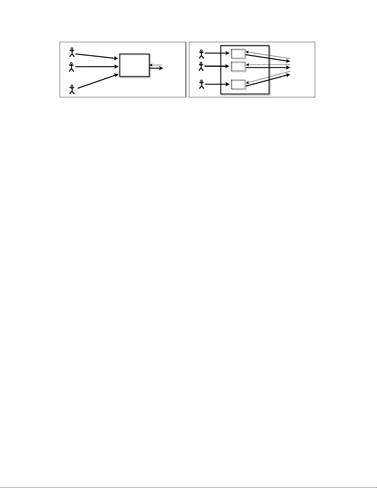
What Can W e Learn Pri v ately? ∗ Shi va Prasad Kasi viswanathan † Homin K. Lee ‡ K obbi Nissim § Sofya Raskhodniko va ¶ Adam Smith ¶ February 13, 2013 Abstract Learning problems form an important category of computational tasks that generalizes many of the computations researchers apply to large real-life data sets. W e ask: what concept classes can be learned priv ately , namely , by an algorithm whose output does not depend too heavily on an y one input or specific training example? More precisely , we in vestigate learning algorithms that satisfy differ ential privacy , a notion that provides strong confidentiality guarantees in contexts where aggreg ate information is released about a database containing sensitiv e information about individuals. Our goal is a broad understanding of the resources required for priv ate learning in terms of samples, computation time, and interaction. W e demonstrate that, ignoring computational constraints, it is pos- sible to priv ately agnostically learn any concept class using a sample size approximately logarithmic in the cardinality of the concept class. Therefore, almost anything learnable is learnable pri vately: specif- ically , if a concept class is learnable by a (non-priv ate) algorithm with polynomial sample comple xity and output size, then it can be learned pri vately using a polynomial number of samples. W e also present a computationally efficient pri vate P A C learner for the class of parity functions. This result dispels the similarity between learning with noise and private learning (both must be rob ust to small changes in inputs), since parity is thought to be very hard to learn gi ven random classification noise. Local (or randomized response ) algorithms are a practical class of pri vate algorithms that have re- ceiv ed extensi ve in vestigation. W e provide a precise characterization of local pri v ate learning algorithms. W e show that a concept class is learnable by a local algorithm if and only if it is learnable in the statis- tical query (SQ) model. Therefore, for local pri vate learning algorithms, the similarity to learning with noise is stronger: local learning is equiv alent to SQ learning, and SQ algorithms include most kno wn noise-tolerant learning algorithms. Finally , we present a separation between the power of interactive and noninteractive local learning algorithms. Because of the equiv alence to SQ learning, this result also separates adaptive and nonadaptive SQ learning. 1 Intr oduction The data pri vac y problem in modern databases is similar to that faced by statistical agencies and medical researchers: to learn and publish global analyses of a population while maintaining the confidentiality of the ∗ A preliminary version of this paper appeared in 49th Annual IEEE Symposium on F oundations of Computer Science [37]. † CCS-3, Los Alamos National Laboratory . Part of this w ork done while a student at Pennsylv ania State Uni versity and supported by NSF award CCF-072891. ‡ Department of Computer Science, Columbia Univ ersity , hkl7@columbia.edu § Department of Computer Science, Ben-Gurion University , kobbi@cs.bgu.ac.il. Supported in part by the Israel Science Foun- dation (grant 860/06), and by the Frankel Center for Computer Science. ¶ Department of Computer Science and Engineering, Pennsylv ania State Uni versity , { sofya,asmith } @cse.psu.edu. S.R. and A.S. are supported in part by NSF award CCF-0729171. 1 participants in a surv ey . There is a v ast body of work on this problem in statistics and computer science. Ho wev er , until recently , most schemes proposed in the literature lacked rigorous analysis of priv acy and utility . A recent line of work [29, 26, 11, 24, 22, 21, 47, 25, 44, 7, 48, 14, 27] , initiated by Dinur and Nissim [20] and called private data analysis , seeks to place data priv acy on firmer theoretical foundations and has been successful at formulating a strong, yet attainable priv acy definition. The notion of differ ential privacy [24] that emer ged from this line of w ork provides rigorous guarantees e ven in the presence of a malicious adv er- sary with access to arbitrary auxiliary information. It requires that whether an individual supplies her actual or fake information has almost no ef fect on the outcome of the analysis. Gi ven this definition, it is natural to ask: what computational tasks can be performed while maintaining pri vac y? Research on data pri v acy , to the extent that it formalizes precise goals, has mostly focused on function evaluation (“what is the value of f (z) ?”), namely , ho w much pri vac y is possible if one wishes to release (an approximation to) a particular function f , ev aluated on the database z . (A notable exception is the recent work of McSherry and T alwar , using differential priv acy in the design of auction mechanisms [44]). Our goal is to expand the utility of priv ate protocols by examining which other computational tasks can be performed in a pri vac y-preserving manner . Private Learning. Learning problems form an important category of computational tasks that generalizes many of the computations researchers apply to large real-life data sets. In this work, we ask what can be learned privately , namely , by an algorithm whose output does not depend too hea vily on any one input or specific training example. Our goal is a broad understanding of the resources required for pri v ate learning in terms of samples, computation time, and interaction. W e examine two basic notions from computational learning theory: V aliant’ s probabilistically approximately correct (P AC) learning [51] model and Kearns’ statistical query (SQ) model [39]. Informally , a concept is a function from e xamples to labels, and a class of concepts is learnable if for an y distribution D on examples, one can, gi ven limited access to examples sampled from D labeled according to some tar get concept c , find a small circuit (hypothesis) which predicts c ’ s labels with high probability ov er future examples taken from the same distribution. In the P A C model, a learning algorithm can access a polynomial number of labeled examples. In the SQ model, instead of accessing examples directly , the learner can specify some properties (i.e., predicates) on the examples, for which he is gi ven an estimate, up to an additiv e polynomially small error , of the probability that a random e xample chosen from D satisfies the property . P A C learning is strictly stronger than the SQ learning [39]. W e model a statistical database as a vector z = ( z 1 , · · · , z n ) , where each entry has been contributed by an individual. When analyzing how well a priv ate algorithm learns a concept class, we assume that entries z i of the database are random examples generated i.i.d. from the underlying distribution D and labeled by a tar get concept c . This is exactly ho w (not necessarily pri vate) learners are analyzed. F or instance, an example might consist of an individual’ s gender , age, and blood pressure history , and the label, whether this indi vidual has had a heart attack. The algorithm has to learn to predict whether an indi vidual has had a heart attack, based on gender , age, and blood pressure history , generated according to D . W e require a priv ate algorithm to keep entire examples (not only the labels) confidential. In the scenario abov e, it translates to not rev ealing each participant’ s gender , age, blood pressure history , and heart attack incidence. More precisely , the output of a priv ate learner should not be significantly affected if a partic- ular example z i is replaced with arbitrary z 0 i , for all z i and z 0 i . In contrast to correctness or utility , which is analyzed with respect to distrib ution D , differential priv acy is a worst-case notion. Hence, when we analyze the pri v acy of our learners we do not make an y assumptions on the underlying distribution. Such as- 2 sumptions are fragile and, in particular , would fall apart in the presence of auxiliary knowledge (also called background kno wledge or side information) that the adversary might hav e: conditioned on the adversary’ s auxiliary kno wledge, the distribution ov er examples might look v ery different from D . 1.1 Our Contributions W e introduce and formulate priv ate learning problems, as discussed abov e, and develop novel algorithmic tools and bounds on the sample size required by priv ate learning algorithms. Our results paint a picture of the classes of learning problems that are solv able subject to priv acy constraints. Specifically , we pro vide: (1) A Pri vate V ersion of Occam’ s Razor . W e present a generic pri v ate learning algorithm. For any concept class C , we giv e a distribution-free differentially-pri vate agnostic P A C learner for C that uses a number of samples proportional to log |C | . This is a priv ate analogue of the “cardinality version” of Occam’ s razor , a basic sample comple xity bound from (non-priv ate) learning theory . The sample complexity of our version is similar to that of the original, although the priv ate algorithm is very dif ferent. As in Occam’ s razor, the learning algorithm is not necessarily computationally ef ficient. (2) An Efficient Pri vate Lear ner f or Parity . W e give a computationally ef ficient, distribution-free dif- ferentially priv ate P A C learner for the class of parity functions 1 ov er { 0 , 1 } d . The sample and time complexity are comparable to that of the best non-pri v ate learner . (3) Equivalence of Local (“Randomized Response”) and SQ Learning . W e precisely characterize the po wer of local , or r andomized r esponse , pri v ate learning algorithms. Local algorithms are a special (practical) class of priv ate algorithms and are popular in the data mining and statistics literature [53, 2, 1, 3, 52, 29, 45, 36]. They add randomness to each indi vidual’ s data independently before processing the input. W e show that a concept class is learnable by a local differentially pri vate algorithm if and only if it is learnable in the statistical query (SQ) model. This equiv alence relates notions that were conceiv ed in very dif ferent contexts. (4) Separation of Interactive and Noninteractive Local Learning. Local algorithms can be noninterac- tive , that is, using one round of interaction with indi viduals holding the data, or interactive , that is, using more than one round (and in each recei ving randomized responses from indi viduals). W e construct a concept class, called masked-parity , that is ef ficiently learnable by inter active local algorithms under the uniform distribution on examples, but requires an exponential (in the dimension) number of samples to be learned by a noninter active local algorithm. The equiv alence (3) of local and SQ learning shows that interaction in local algorithms corresponds to adaptivity in SQ algorithms. The masked-parity class thus also separates adapti ve and nonadapti ve SQ learning. 1.1.1 Implications “Anything” learnable is privately learnable using few samples. The generic agnostic learner (1) has an important consequence: if some concept class C is learnable by an y algorithm, not necessarily a priv ate one, whose output length in bits is polynomially bounded, then C is learnable priv ately using a polynomial num- ber of samples (possibly in exponential time). This result establishes the basic feasibility of pri vate learning: it was not clear a priori ho w sev erely priv acy af fects sample complexity , ev en ignoring computation time. 1 While the generic learning result (1) extends easily to “agnostic” learning (defined belo w), the learner for parity does not. The limitation is not surprising, since ev en non-priv ate agnostic learning of parity is at least as hard as learning parity with random noise. 3 User x 1 x n . . . R x 1 x n . . . A x 2 R R User x 2 (a) (b) A F igur e 1: T wo basic models for database priv acy: (a) the centralized model, in which data is collected by a trusted agency that publishes aggregate statistics or answers users’ queries; (b) the local model, in which users retain their data and run a randomization procedure locally to produce output which is safe for publication. The dotted arrows from users to data holders indicate that protocols may be completely noninteractiv e: in this case there is a single publication, without feedback from users. Learning with noise is different from private learning . There is an intuitively appealing similarity be- tween learning from noisy examples and pri vate learning: algorithms for both problems must be robust to small v ariations in the data. This apparent similarity is strengthened by a result of Blum, Dwork, McSherry and Nissim [11] showing that any algorithm in Kearns’ statistical query (SQ) model [39] can be imple- mented in a dif ferentially priv ate manner . SQ was introduced to capture a class of noise-resistant learning algorithms. These algorithms access their input only through a sequence of approximate averaging queries. One can privately approximate the average of a function with values in [0 , 1] ov er the data set of n individu- als to within additiv e error O (1 /n ) (Dwork and Nissim [26]). Thus, one can simulate the behavior of an SQ algorithm pri vately , query by query . Our efficient pri vate learner for parity (2) dispels the similarity between learning with noise and priv ate learning. First, SQ algorithms pro vably require e xponentially man y (in the dimension) queries to learn parity [39]. More compellingly , learning parity with noise is thought to be computationally hard, and has been used as the basis of se veral cryptographic primiti ves ( e.g ., [13, 35, 4, 49]). Limitations of local (“randomized response”) algorithms. Local algorithms (also referred to as ran- domized r esponse , input perturbation , P ost Randomization Method ( PRAM ) , and F rame work for High- Accuracy Strict-Privacy Pr eserving Mining ( FRAPP ) ) have been studied extensi vely in the context of priv acy- preserving data mining, both in statistics and computer science ( e.g., [53, 2, 1, 3, 52, 29, 45, 36]). Roughly , a local algorithm accesses each individual’ s data via independent randomization operators. See Figure 1, p. 4. Local algorithms were introduced to encourage truthfulness in surve ys: respondents who know that their data will be randomized are more likely to answer honestly . For example, W arner [53] famously considered a surve y technique in which respondents are asked to gi ve the correct answer to a sensitiv e (true/false) question with probability 2 / 3 and the incorrect answer with probability 1 / 3 , in the hopes that the added uncertainty would encourage them to answer honestly . The proportion of “true” answers in the population is then estimated using a standard, non-priv ate decon v olution. The accepted pri vac y requirement for local algorithms is equiv alent to imposing differential priv acy on each randomization operator [29]. Local algorithms are popular because they are easy to understand and implement. In the extreme case, users can retain their data and apply the randomization operator themselves, using a physical device [53, 46] or a cryptographic protocol [5]. The equi valence between local and SQ algorithms (3) is a powerful tool that allows us to apply results 4 from learning theory . In particular , since parity is not learnable with a small number of SQ queries [39] but is P AC learnable pri vately (2) , we get that local algorithms require exponentially more data for some learning tasks than do general priv ate algorithms. Our results also imply that local algorithms are strictly less po werful than (non-priv ate) algorithms for learning with classification noise because subexponential (non-pri vate) algorithms can learn parity with noise [13]. Adaptivity in SQ algorithms is important. Just as local algorithms can be interacti ve, SQ algorithms can be adaptive , that is, the averaging queries they make may depend on answers to previous queries. The equi valence of SQ and local algorithms (3) preserv es interaction/adaptivity: a concept class is nonadapti v ely SQ learnable if and only if it is noninteractiv ely locally learnable. The masked parity class (4) sho ws that interaction (resp., adapti vity) adds considerable power to local (resp., SQ) algorithms. Most of the reasons that local algorithms are so attractive in practice, and have receiv ed such attention, apply only to noninteracti ve algorithms (interaction can be costly , complicated, or ev en impossible—for instance, when statistical information is collected by an intervie wer , or at a polling booth). This suggests that further in vestigating the power of nonadaptive SQ learners is an important problem. For e xample, the SQ algorithm for learning conjunctions [42] is nonadapti ve, but SQ formulations of the perceptron and k -means algorithms [11] seem to rely hea vily on adaptivity . Understanding the “price” of privacy f or lear ning pr oblems. The SQ result of Blum et al. [11] and our learner for parity (2) provide efficient (i.e., polynomial time) priv ate learners for essentially all the concept classes known (by us) to have ef ficient non-pri vate distribution-free learners. Finding a concept class that can be learned ef ficiently , but not priv ately and ef ficiently , remains an interesting and important question. Our results also lead to questions of optimal sample complexity for learning problems of practical im- portance. The priv ate simulation of SQ algorithms due to Blum et al. [11] uses a factor of approximately √ t/ more data points than the na ¨ ıve non-pri v ate implementation, where t is the number of SQ queries and  is the parameter of differential priv acy (typically a small constant). In contrast, the generic agnostic learner (1) uses a factor of at most 1 / more samples than the corresponding non-pri vate learner . For parity , our pri vate learner uses a factor of roughly 1 / more samples than, and about the same computation time as, the non-pri vate learner . What, then, is the additional cost of priv acy when learning practical concept classes (half-planes, lo w-dimensional curves, etc)? Can the theoretical sample bounds of (1) be matched by (more) ef ficient learners? 1.1.2 T echniques Our generic priv ate learner (1) adapts the exponential sampling technique of McSherry and T alwar [44], de veloped in the conte xt of auction design. Our use of the exponential mechanism inspired an elegant subsequent result of Blum, Liggett, and Roth [14] (BLR) on simultaneously approximating many different functions. The efficient pri vate learner for parity (2) uses a very different technique, based on sampling, running a non-pri vate learner , and occasionally refusing to answer based on delicately calibrated probabilities. Run- ning a non-pri vate learner on a random subset of examples is a very intuitiv e approach to b uilding pri vate algorithms, but it is not priv ate in general. The priv ate learner for parity illustrates both why this technique can leak pri vate information and ho w it can sometimes be repaired based on special (in this case, algebraic) structure. 5 The interesting direction of the equiv alence between SQ and local learners (3) is proved via a simulation of any local algorithm by a corresponding SQ algorithm. W e found this simulation surprising since local protocols can, in general, hav e very complex structure (see, e.g ., [29]). The SQ algorithm proceeds by a direct simulation of the output of the randomization operators. F or a giv en input distribution D and an y operator R , one can sample from the corresponding output distrib ution R ( D ) via rejection sampling. W e sho w that if R is dif ferentially priv ate, the rejection probabilities can be approximated via low-accuracy SQ queries to D . Finally , the separation between adaptiv e and nonadaptiv e SQ (4) uses a Fourier analytic argument in- spired by K earns’ SQ lower bound for parity [39]. 1.1.3 Classes of Private Learning Algorithms LNI ∗ = NASQ ∗ LI ∗ = SQ ∗ PP A C ∗ = P AC ∗ P ARITY MASKED-P ARITY F igur e 2: Relationships among learning classes taking into account sample complexity , but not computational ef ficiency . W e can summarize our results via a complexity-theoretic picture of learnable and pri vately learnable concept classes (more precisely , the members of the classes are pairs of concept classes and example dis- tributions). In order to make asymptotic statements, we measure complexity in terms of the length d of the binary description of examples. W e first consider learners that use a polynomial (in d ) number of samples and output a hypothesis that is described using a polynomial number of bits, but have unlimited computation time. Let P A C ∗ denote the set of concept classes that are learnable by such algorithms ignoring priv acy , and let PP A C ∗ denote the subset of P A C ∗ learnable by dif ferentially priv ate 2 algorithms. Since we restrict the learner’ s output to a polynomial number of bits, the hypothesis classes of the algorithms are de facto limited to have size at most exp( pol y ( d )) . Thus, the generic priv ate learner (point (1) in the introduction) will use a polynomial number of samples, and P A C ∗ = PP A C ∗ . W e can similarly interpret the other results above. W ithin P A C ∗ , we can consider subsets of concepts learnable by SQ algorithms ( SQ ∗ ), nonadapti ve SQ algorithms ( NASQ ∗ ), local interacti ve algorithms ( LI ∗ ) and local noninteracti ve algorithms ( LNI ∗ ). W e obtain the following picture (see page 6): LNI ∗ = NASQ ∗ ( LI ∗ = SQ ∗ ( PP A C ∗ = P A C ∗ . The equality of LI ∗ and SQ ∗ , and of LNI ∗ and NASQ ∗ , follow from the SQ simulation of local algorithms (Theorem 5.14). The parity and masked-parity concept classes separate PP A C ∗ from SQ ∗ and SQ ∗ from NASQ ∗ , respecti vely (Corollaries 5.15 and 5.17). ( Note: The separation of PP A C ∗ from SQ ∗ holds ev en for distrib ution-free learning; in contrast, the separation of SQ ∗ from NASQ ∗ holds for learnability under a 2 Differential priv acy is quantified by a real parameter  > 0 . T o make qualitativ e statements, we look at algorithms where  → 0 as d → ∞ . T aking  = 1 /d c for any constant c > 0 would yield the same class. 6 specific distribution on examples, since the adaptive SQ learner for MASKED-P ARITY requires a uniform distribution on e xamples.) When we take computational ef ficiency into account, the picture changes. The relation between local and SQ classes remain the same modulo a technical restriction on the randomization operators (Defini- tion 5.13). SQ remains distinct from PP A C since parity is ef ficiently learnable pri v ately . Ho we ver , it is an open question whether concept classes which can be ef ficiently learned can also be ef ficiently learned pri vately . 1.2 Related W ork Prior to this work, the literature on differential priv acy studied function approximation tasks (e.g. [20, 26, 11, 24, 47, 7]), with the e xception of the work of McSherry and T alwar on mechanism design [44]. Ne vertheless, sev eral of these prior results hav e direct implications to machine learning-related problems. Blum et al. [11] considered a particular class of learning algorithms (SQ), and showed that algorithms in the class could be simulated using noisy function ev aluations. In an independent, unpublished work, Chaudhuri, Dwork, and T alwar considered a version of pri vate learning in which pri vac y is afforded only to input labels, but not to examples. Other works considered specific machine learning problems such as mining frequent itemsets [29], k -means clustering [11, 47], learning decision trees [11], and learning mixtures of Gaussians [47]. As mentioned abov e, a subsequent result of Blum, Ligett and Roth [14] on approximating classes of lo w-VC-dimension functions was inspired by our generic agnostic learner . W e discuss their result further in Section 3.1. Since the original v ersion of our work, there hav e also been sev eral results connecting dif ferential priv acy to more “statistical” notions of utility , such as consistency of point estimation and density estimation [50, 23, 54, 56]. Our separation of interacti ve and noninteractiv e protocols in the local model (3) also has a precedent: Dwork et al. [24] separated interactive and noninteractiv e priv ate protocols in the centralized model, where the user accesses the data via a server that runs differentially priv ate algorithms on the database and sends back the answers. That separation has a very different flavor from the one in this work: any example of a computation that cannot be performed noninteractiv ely in the centralized model must rely on the fact that the computational task is not defined until after the first answer from the serv er is receiv ed. (Otherwise, the user can send an algorithm for that task to the server holding the data, thus obviating the need for interaction.) In contrast, we present a computational task that is hard for noninteractiv e local algorithms – learning masked parity – yet is defined in adv ance. In the machine learning literature, several notions similar to dif ferential priv acy hav e been explored under the rubric of “algorithmic stability” [19, 40, 16, 43, 28, 9]. The most closely related notion is change- one err or stability , which measures how much the generalization error changes when an input is changed (see the surv ey [43]). In contrast, differential priv acy measures ho w the distrib ution o ver the entire output changes—a more complex measure of stability (in particular, differential priv acy implies change-one error stability). A dif ferent notion, stability under resampling of the data from a gi ven distrib ution [10, 9], is con- nected to the sample-and-aggregate method of [47] but is not directly rele vant to the techniques considered here. Finally , in a different vein, Freund, Mansour and Schapire [31] used a weighted averaging technique with the same weights as the sampler in our generic learner to reduce generalization error (see Section 3.1). 7 2 Pr eliminaries W e use [ n ] to denote the set { 1 , 2 , . . . , n } . Logarithms base 2 and base e are denoted by log and ln , respec- ti vely . Pr[ · ] and E [ · ] denote probability and expectation, respecti vely . A ( x ) is the probability distrib ution ov er outputs of a randomized algorithm A on input x . The statistical dif fer ence between distrib utions P and Q on a discrete space D is defined as max S ⊂ D | P ( S ) − Q ( S ) | . 2.1 Differential Pri vacy A statistical database is a vector z = ( z 1 , . . . , z n ) ov er a domain D , where each entry z i ∈ D represents information contributed by one individual. Databases z and z 0 are neighbors if z i 6 = z 0 i for exactly one i ∈ [ n ] (i.e., the Hamming distance between z and z 0 is 1). All our algorithms are symmetric, that is, the y do not depend on the order of entries in the database z . Thus, we could define a database as a multi-set in D , and use symmetric difference instead of the Hamming metric to measure distance. W e adhere to the vector formulation for consistency with the pre vious works. A (randomized) algorithm (in our context, this will usually be a learning algorithm) is priv ate if neigh- boring databases induce nearby distributions on its outcomes: Definition 2.1 (  -dif ferential pri vac y [24]) . A randomized algorithm A is  -differ entially private if for all neighboring databases z , z 0 , and for all sets S of outputs, Pr[ A (z) ∈ S ] ≤ exp(  ) · Pr[ A (z 0 ) ∈ S ] . The pr obability is taken o ver the random coins of A . In [24], the notion above was called “indistinguishability”. The name “differential priv acy” was sug- gested by Mike Schroeder , and first appeared in Dwork [21]. Dif ferential priv acy composes well (see, e .g., [22, 47, 44, 38]): Claim 2.2 (Composition and Post-processing) . If a randomized algorithm A runs k algorithms A 1 , ..., A k , wher e each A i is  i -differ entially private, and outputs a function of the results (that is, A (z) = g ( A 1 (z) , A 2 (z) , ..., A k (z)) for some pr obabilistic algorithm g ), then A is ( P k i =1  i ) -differ entially private. One method for obtaining ef ficient dif ferentially priv ate algorithms for approximating real-valued func- tions is based on adding Laplacian noise to the true answer . Let Lap( λ ) denote the Laplace probability distribution with mean 0 , standard de viation √ 2 λ , and p.d.f. f ( x ) = 1 2 λ e −| x | /λ . Theorem 2.3 (Dwork et al. [24]) . F or a function f : D n → R , define its global sensitivity GS f = max z , z 0 | f (z) − f (z 0 ) | where the maximum is over all neighboring databases z , z 0 . Then, an algorithm that on input z returns f (z) + η wher e η ∼ Lap( GS f / ) is  -differ entially private. 2.2 Preliminaries fr om Learning Theory A concept is a function that labels examples taken from the domain X by the elements of the range Y . A concept class C is a set of concepts. It comes implicitly with a way to represent concepts; size ( c ) is the size of the (smallest) representation of c under the giv en representation scheme. The domain and the range of the concepts in C are understood to be ensembles X = { X d } d ∈ N and Y = { Y d } d ∈ N , where the representation of elements in X d , Y d is of size at most d . W e focus on binary classification problems, in which the label space Y d is { 0 , 1 } or { +1 , − 1 } ; the parameter d thus measures the size of the e xamples 8 in X d . (W e use the parameter d to formulate asymptotic complexity notions.) The concept classes are ensembles C = {C d } d ∈ N where C d is the class of concepts from X d to Y d . When the size parameter is clear from the context or not important, we omit the subscript in X d , Y d , C d . Let D be a distribution ov er labeled examples in X d × Y d . A learning algorithm is gi ven access to D (the method for accessing D depends on the type of learning algorithm). It outputs a hypothesis h : X d → Y d from a hypothesis class H = {H d } d ∈ N . The goal is to minimize the misclassification err or of h on D , defined as err ( h ) = Pr ( x,y ) ∼D [ h ( x ) 6 = y ] . The success of a learning algorithm is quantified by parameters α and β , where α is the desired error and β bounds the probability of failure to output a hypothesis with this error . Error measures other than misclassification are considered in supervised learning ( e.g ., L 2 2 ). W e study only misclassification error here, since for binary labels it is equi valent to the other common error measures. A learning algorithm is usually giv en access to an oracle that produces i.i.d. samples from D . Equiv- alently , one can vie w the learning algorithm’ s input as a list of n labeled examples, i.e., z ∈ D n where D = X d × Y d . P A C learning and agnostic learning are described in Definitions 2.4 and 2.5. Another common method of access to D is via “statistical queries”, which return the approximate av erage of a func- tion over the distribution. Algorithms that work in this model can be simulated gi ven i.i.d. examples. See Section 5. P A C learning algorithms are frequently designed assuming a promise that the examples are labeled consistently with some tar get concept c from a class C : namely , c ∈ C d and y = c ( x ) for all ( x, y ) in the support of D . In that case, we can think of D as a distribution only ov er examples X d . T o avoid ambiguity , we use X to denote a distrib ution over X d . In the P A C setting, err ( h ) = Pr x ∼X [ h ( x ) 6 = c ( x )] . Definition 2.4 (P AC Learning) . A concept class C over X is P A C learnable using hypothesis class H if ther e exist an algorithm A and a polynomial poly ( · , · , · ) such that for all d ∈ N , all concepts c ∈ C d , all distributions X on X d , and all α, β ∈ (0 , 1 / 2) , given inputs α, β and z = ( z 1 , · · · , z n ) , where n = poly ( d, 1 /α, log(1 /β )) , z i = ( x i , c ( x i )) and x i ar e drawn i.i.d. fr om X for i ∈ [ n ] , algorithm A outputs a hypothesis h ∈ H satisfying Pr[ err ( h ) ≤ α ] ≥ 1 − β . (1) The pr obability is taken o ver the random choice of the e xamples z and the coin tosses of A . Class C is (inefficiently) P A C learnable if there exists some hypothesis class H and a P A C learner A such that A P AC learns C using H . Class C is efficiently P A C learnable if A runs it time polynomial in d, 1 /α , and log(1 /β ) . Remark: Our definition deviates slightly from the standard one (see, e.g ., [42]) in that we do not take into consideration the size of the concept c . This choice allo ws us to treat P A C learners and agnostic learners identically . One can change Definition 2.4 so that the number of samples depends polynomially also on the size of c without affecting any of our results significantly . Agnostic learning [32, 41] is an extension of P A C learning that remov es assumptions about the target concept. Roughly speaking, the goal of an agnostic learner for a concept class C is to output a hypothesis h ∈ H whose error with respect to the distribution is close to the optimal possible by a function from C . In the agnostic setting, err ( h ) = Pr ( x,y ) ∼D [ h ( x ) 6 = y ] . 9 Definition 2.5 (Agnostic Learning) . (Ef ficiently) agnostically learnable is defined identically to (ef ficiently) P A C learnable with two e xceptions: (i) the data ar e dr awn fr om an arbitrary distribution D on X d × Y d ; (ii) instead of Equation 1, the output of A has to satisfy: Pr[ err ( h ) ≤ O P T + α ] ≥ 1 − β , wher e O P T = min f ∈C d { err ( f ) } . As before , the pr obability is taken over the random choice of z , and the coin tosses of A . Definitions 2.4 and 2.5 capture distribution-fr ee learning, in that they do not assume a particular form for the distributions X or D . In Section 5.3, we also consider learning algorithms that assume a specific distribution D on examples (but make no assumption on which concept in C labels the examples). When we discuss such algorithms, we specify D explicitly; without qualification, “learning” refers to distribution-free learning. Efficiency Measures. The definitions above are suf ficiently detailed to allo w for exact complexity state- ments ( e.g., “ A learns C using n ( α, β ) e xamples and time O ( t ) ”), and the upper and lo wer bounds in this paper are all stated in this language. Howe ver , we also focus on two broader measures to allow for qualitati ve statements: (a) polynomial sample complexity is the default notion in our definitions. W ith the novel restric- tion of priv acy , it is not a priori clear which concept classes can be learned using few examples even if we ignore computation time. (b) W e use the term efficient priv ate learning to impose the additional restriction of polynomial computation time (which implies polynomial sample complexity). 3 Priv ate P A C and Agnostic Learning W e define priv ate P A C learners as algorithms that satisfy definitions of both differential priv acy and P A C learning. W e emphasize that these are qualitativ ely different requirements. Learning must succeed on av erage over a set of examples drawn i.i.d. from D (often under the additional promise that D is consistent with a concept from a target class). Differential priv acy , in contrast, must hold in the worst case, with no assumptions on consistency . Definition 3.1 (Pri vate P A C Learning) . Let d, α, β be as in Definition 2.4 and  > 0 . Concept class C is (inefficiently) priv ately P A C learnable using hypothesis class H if ther e exists an algorithm A that takes inputs , α, β , z , where n , the number of labeled examples in z , is polynomial in 1 /, d, 1 /α, log(1 /β ) , and satisfies a. [ Privacy ] F or all  > 0 , algorithm A ( , · , · , · ) is  -dif fer entially private (Definition 2.1); b . [ Utility ] Algorithm A P AC learns C using H (Definition 2.4). C is ef ficiently privately P AC learnable if A runs in time polynomial in d, 1 /, 1 /α , and log (1 /β ) . Definition 3.2 (Pri vate Agnostic Learning) . (Efficient) priv ate agnostic learning is defined analogously to (efficient) private P AC learning with Definition 2.5 r eplacing Definition 2.4 in the utility condition. Ev aluating the quality of a particular hypothesis is easy: one can pri vately compute the fraction of the data it classifies correctly (enabling cross-validation) using the sum query framework of [11]. The dif ficulty of constructing priv ate learners lies in finding a good hypothesis in what is typically an exponentially large space. 10 3.1 A Generic Private Agnostic Lear ner In this section, we present a priv ate analogue of a basic consistent learning result, often called the cardinality version of Occam’ s razor 3 . This classical result shows that a P A C learner can weed out all bad hypotheses gi ven a number of labeled examples that is logarithmic in the size of the hypothesis class (see [42, p. 35]). Our generic pri vate learner is based on the e xponential mechanism of McSherry and T alwar [44]. Let q : D n × H d → R take a database z and a candidate hypothesis h , and assign it a score q (z , h ) = −|{ i : x i is misclassified by h, i.e., y i 6 = h ( x i ) }| . That is, the score is minus the number of points in z misclassified by h . The classic Occam’ s razor argument assumes a learner that selects a hypothesis with maximum score (that is, minimum empirical error). Instead, our pri vate learner A  q is defined to sample a random hypothesis with probability dependent on its score: A  q (z) : Output hypothesis h ∈ H d with probability proportional to exp  q (z ,h ) 2  . Since the score ranges from − n to 0, hypotheses with low empirical error are exponentially more likely to be selected than ones with high error . Algorithm A  q fits the framework of McSherry and T alwar , and so is  -differentially priv ate. This follows from the fact that changing one entry z i in the database z can change the score by at most 1. Lemma 3.3 (follo wing [44]) . The algorithm A  q is  -differ entially private. A similar exponential weighting algorithm was considered by Freund, Mansour and Schapire [31] for constructing binary classifiers with good generalization error bounds. W e are not aware of any direct connec- tion between the two results. Also note that, except for the case where |H d | is polynomial, the exponential mechanism A  q (z) does not necessarily yield a polynomial time algorithm. Theorem 3.4 (Generic Priv ate Learner) . F or all d ∈ N , any concept class C d whose car dinality is at most exp(p oly( d )) is privately agnostically learnable using H d = C d . Mor e pr ecisely , the learner uses n = O ((ln |H d | + ln 1 β ) · max { 1 α , 1 α 2 } ) labeled examples fr om D , wher e , α , and β are parameters of the private learner . (The learner might not be efficient.) Pr oof. Let A  q be as defined abov e. The pri vac y condition in Definition 3.1 is satisfied by Lemma 3.3. W e now sho w that the utility condition is also satisfied. Consider the ev ent E = {A  q (z) = h with err ( h ) > α + O P T } . W e want to prov e that Pr[ E ] ≤ β . Define the training error of h as err T ( h ) =   { i ∈ [ n ] | h ( x i ) 6 = y i }   /n = − q (z , h ) /n . By Chernof f-Hoeffding bounds (see Theorem A.2 in Appendix A), Pr  | err ( h ) − err T ( h ) | ≥ ρ  ≤ 2 exp( − 2 nρ 2 ) for all hypotheses h ∈ H d . Hence, Pr  | err ( h ) − err T ( h ) | ≥ ρ for some h ∈ H d  ≤ 2 |H d | exp( − 2 nρ 2 ) . 3 W e discuss the relationship to the “compression version” of Occam’ s razor at the end of this section. 11 W e now analyze A  q (z) conditioned on the event that for all h ∈ H d , | err ( h ) − err T ( h ) | < ρ . For e very h ∈ H d , the probability that A  q (z) = h is exp( −  2 · n · err T ( h )) P h 0 ∈H d exp( −  2 · n · err T ( h 0 )) ≤ exp  −  2 · n · err T ( h )  max h 0 ∈H d exp( −  2 · n · err T ( h 0 )) = exp  −  2 · n · ( err T ( h ) − min h 0 ∈H d err T ( h 0 ))  ≤ exp  −  2 · n · ( err T ( h ) − ( O P T + ρ ))  . Hence, the probability that A  q (z) outputs a hypothesis h ∈ H d such that err T ( h ) ≥ O P T + 2 ρ is at most |H d | exp( − nρ/ 2) . No w set ρ = α/ 3 . If err ( h ) ≥ O P T + α then | err ( h ) − err T ( h ) | ≥ α/ 3 or err T ( h ) ≥ O P T + 2 α/ 3 . Thus Pr[ E ] ≤ |H d | (2 exp( − 2 nα 2 / 9) + exp( − nα/ 6)) ≤ β where the last inequality holds for n ≥ 6  (ln |H d | + ln 1 β ) · max { 1 α , 1 α 2 }  . Remark: In the non-priv ate agnostic case, the standard Occam’ s razor bound guarantees that O ((log |C d | + log(1 /β )) /α 2 ) labeled examples suf fice to agnostically learn a concept class C d . The bound of Theorem 3.4 dif fers by a factor of O ( α  ) if α >  , and does not differ at all otherwise. F or (non-agnostic) P A C learning, the dependence on α in the sample size for both the pri vate and non-priv ate v ersions impro ves to 1 /α . In that case the upper bounds for priv ate and non-priv ate learners dif fer by a factor of O (1 / ) . Finally , the theorem can be extended to settings where H d 6 = C d , but in this case using the same sample complexity the learner outputs a hypothesis whose error is close to the best error attainable by a function in H d . Implications of the Private Agnostic Lear ner The priv ate agnostic learner has the follo wing important consequence: If some concept class C d is learnable by any algorithm A , not necessarily a priv ate one, and A ’ s output length in bits is polynomially bounded, then there is a (possibly exponential time) priv ate algorithm that learns C d using a polynomial number of samples. Since A ’ s output is polynomially long, A ’ s hypothesis class H d must hav e size at most 2 poly ( d ) . Since A learns C d using H d , class H d must contain a good hypothesis. Thus, our pri v ate learner will learn C d using H d with sample comple xity linear in log |H d | . The “compr ession version” of Occam’ s razor It is most natural to state our result as an analogue of the cardinality version of Occam’ s razor , which bounds generalization error in terms of the size of the hypothesis class. Howe ver , our result can be e xtended to the compression version, which captures the general relationship between compression and learning (we borro w the “cardinality version” terminology from [42]). This latter v ersion states that an y algorithm which “compresses” the data set, in the sense that it finds a consistent hypothesis which has a short description relative to the number of samples seen so far , is a good learner (see [15] and [42, p. 34]). Compression by itself does not imply priv acy , because the compression algorithm’ s output might encode a fe w examples in the clear (for e xample, the hyperplane output by a support vector machine is defined via a small number of actual data points). Ho wev er , Theorem 3.4 can be extended to provide a priv ate analogue of the compression version of Occam’ s razor . If there exists an algorithm that compresses, in the sense above, then there also exists a priv ate P A C learner which does not have fixed sample complexity , but uses an expected number of samples similar to that of the compression algorithm. The priv ate learner proceeds in rounds: at each round it requests twice as many examples as in the previous round, and uses a 12 restricted hypothesis class consisting of sufficiently concise hypotheses from the original class H . W e omit the straightforward details. 3.2 Private Lear ning with VC dimension Sample Bounds In the non-priv ate case one can also bound the sample size of a P AC learner in terms of the V apnik- Chervonenkis (VC) dimension of the concept class. Definition 3.5 (VC dimension) . A set S ⊆ X d is shattered by a concept class C d if C d r estricted to S contains all 2 | S | possible functions fr om S to { 0 , 1 } . The VC dimension of C d , denoted V C D I M ( C d ) , is the car dinality of a lar gest set S shattered by C d . W e can extend Theorem 3.4 to classes with finite VC dimension, but the resulting sample complexity also depends logarithmically on the size of the domain from which examples are drawn. Recent results of Beimel et al. [8] show that for “proper” learning, the dependency is in fact necessary; that is, the VC dimension alone is not sufficient to bound the sample complexity of proper priv ate learning. It is unclear if the dependency is necessary in general. Corollary 3.6. Every concept class C d is privately agnostically learnable using hypothesis class H d = C d with n = O (( V C DI M ( C d ) · ln | X d | + ln 1 β ) · max { 1 α , 1 α 2 } ) labeled examples fr om D . Her e, , α , and β ar e parameters of the private agnostic learner , and V C D I M ( C d ) is the VC dimension of C d . (The learner is not necessarily efficient.) Pr oof. Sauer’ s lemma (see, e.g . , [42]) implies that there are O ( | X d | V C D I M ( C d ) ) different labelings of X d by functions in C d . W e can thus run the generic learner of the pre vious section with a hypothesis class of size |H d | = O ( | X d | V C D I M ( C d ) ) . The statement follo ws directly . Our original proof of the corollary used a result of Blum, Ligget and Roth [14] (which was inspired, in turn, by our generic learning algorithm) on generating synthetic data. The simpler proof above was pointed out to us by an anonymous re vie wer . Remark: Computability Issues with Generic Learners In their full generality , the generic learning results of the pre vious sections (Theorems 3.4 and 3.6) produce well-defined randomized maps, b ut not nec- essarily “algorithms” in the sense of “functions uniformly computable by T uring machines”. This is because the concept class and example domain may themselves not be computable (nor ev en recognizable) uniformly (imagine, for example, a concept class indexed by elements of the halting problem). It is commonly assumed in the learning literature that elements of the concept class and domain can be computed/recognized by a T uring machine and some bound on the length of their binary representations is kno wn. In this case, the generic learners can be implemented by randomized T uring machines with finite expected running time. 4 An Efficient Priv ate Learner f or P ARITY Let P ARITY be the class of parity functions c r : { 0 , 1 } d → { 0 , 1 } indexed by r ∈ { 0 , 1 } d , where c r ( x ) = r  x denotes the inner product modulo 2 . In this section, we present an ef ficient pri vate P A C learning algorithm for P ARITY . The main result is stated in Theorem 4.4. The standard (non-priv ate) P AC learner for P ARITY [33, 30] looks for the hidden vector r by solving a system of linear equations imposed by examples ( x i , c r ( x i )) that the algorithm sees. It outputs an arbitrary 13 vector consistent with the examples, i.e., in the solution space of the system of linear equations. W e want to design a pri vate algorithm that emulates this behavior . A major difficulty is that the priv ate learner’ s behavior must be specified on all databases z , ev en those which are not consistent with an y single parity function. The standard P A C learner would simply fail in such a situation (we denote failure by the output ⊥ ). In contrast, the probability that a pri vate algorithm f ails must be similar for all neighbors z and z 0 . W e first present a pri v ate algorithm A for learning P ARITY that succeeds only with constant probability . Later we amplify its success probability and get a pri vate P A C learner A ∗ for P ARITY . Intuitiv ely , the reason P ARITY can be learned priv ately is that when a ne w example (corresponding to a new linear constraint) is added, the space of consistent hypotheses shrinks by at most a factor of 2. This holds unless the new constraint is inconsistent with previous constraints. In the latter case, the size of the space of consistent hypotheses goes to 0. Thus, the solution space changes drastically on neighboring inputs only when the algorithm fails (outputs ⊥ ). The fact that algorithm outputs ⊥ on a database z and a valid (non ⊥ ) hypothesis on a neighboring database z 0 might lead to priv acy violations. T o avoid this, our algorithm always outputs ⊥ with probability at least 1 / 2 on an y input (Step 1). A P R I V AT E L E A R N E R F O R P ARITY , A (z ,  ) 1. W ith probability 1 / 2 , output ⊥ and terminate. 2. Construct a set S by picking each element of [ n ] independently with probability p = / 4 . 3. Use Gaussian elimination to solve the system of equations imposed by e xamples, indexed by S : namely , { x i  r = c r ( x i ) : i ∈ S } . Let V S denote the resulting af fine subspace. 4. Pick r ∗ ∈ V S uniformly at random and output c r ∗ ; if V S = ∅ , output ⊥ . The proof of A ’ s utility follows by considering all the possible situations in which the algorithm fails to satisfy the error bound, and by bounding the probabilities with which these situations occur . Lemma 4.1 (Utility of A ) . Let X be a distribution over X = { 0 , 1 } d . Let z = ( z 1 , . . . , z n ) , wher e for all i ∈ [ n ] , the entry z i = ( x i , c ( x i )) with x i drawn i.i.d. fr om X and c ∈ P ARITY . If n ≥ 8 α ( d ln 2 + ln 4) then Pr[ A (z ,  ) = h with err or ( h ) ≤ α ] ≥ 1 4 . Pr oof. By standard ar guments in learning theory [42], | S | ≥ 1 α  d ln 2 + ln 1 β  labeled examples are suf ficient for learning P ARITY with error α and failure probability β . Since A adds each element of [ n ] to S independently with probability p = / 4 , the expected size of S is pn = n/ 4 . By the Chernof f bound (Theorem A.1), | S | ≥ n/ 8 with probability at least 1 − e − n/ 16 . W e set β = 1 4 and pick n such that n/ 8 ≥ 1 α ( d ln 2 + ln 4) . W e no w bound the ov erall success probability . A (z ,  ) = h with err ( h ) ≤ α unless one of the following bad e vents happens: (i) A terminates in Step 1, (ii) A proceeds to Step 2, b ut does not get enough examples: | S | < 1 α ( d ln 2 + ln 4)) , (iii) A gets enough examples, but outputs a hypothesis with error greater than α . The first bad ev ent occurs with probability 1/2. If the lower bound on the database size n is satisfied then the second bad ev ent occurs with probability at most e − n/ 16 / 2 ≤ 1 / 8 . The last inequality follo ws from the bound on n and the fact that α ≤ 1 / 2 . Finally , by our choice of parameters, the last bad ev ent occurs with probability at most β / 2 = 1 / 8 . The claimed bound on the success probability follows. 14 Lemma 4.2 (Pri vac y of A ) . Algorithm A is  -differ entially private. As mentioned above, the key observ ation in the following proof is that including of any single point in the sample set S increases the probability of a hypothesis being output by at most 2. Pr oof. T o sho w that A is  -differentially priv ate, it suf fices to prove that any output of A , either a v alid hypothesis or ⊥ , appears with roughly the same probability on neighboring databases z and z 0 . In the remainder of the proof we fix  , and write A (z) as shorthand for A (z ,  ) . W e have to sho w that Pr[ A (z) = h ] ≤ e  · Pr[ A (z 0 ) = h ] for all neighbors z , z 0 ∈ D n and all hypotheses h ∈ P ARITY ; (2) Pr[ A (z) = ⊥ ] ≤ e  · Pr[ A (z 0 ) = ⊥ ] for all neighbors z , z 0 ∈ D n . (3) W e prov e the correctness of Eqn. (2) first. Let z and z 0 be neighboring databases, and let i denote the entry on which they dif fer . Recall that A adds i to S with probability p . Since z and z 0 dif fer only in the i th entry , Pr[ A (z) = h | i / ∈ S ] = Pr[ A (z 0 ) = h | i / ∈ S ] . Note that if Pr[ A (z 0 ) = h | i / ∈ S ] = 0 , then also Pr[ A (z) = h | i / ∈ S ] = 0 , and hence Pr[ A (z) = h ] = 0 because adding a constraint does not add new vectors to the space of solutions. Otherwise, Pr[ A (z 0 ) = h | i / ∈ S ] > 0 . In this case, we rewrite the probability on z as follo ws: Pr[ A (z) = h ] = p · Pr[ A (z) = h | i ∈ S ] + (1 − p ) · Pr[ A (z) = h | i / ∈ S ] , and apply the same transformation to the probability on z 0 . Then Pr[ A (z) = h ] Pr[ A (z 0 ) = h ] = p · Pr[ A (z) = h | i ∈ S ] + (1 − p ) · Pr[ A (z) = h | i / ∈ S ] p · Pr[ A (z 0 ) = h | i ∈ S ] + (1 − p ) · Pr[ A (z 0 ) = h | i / ∈ S ] ≤ p · Pr[ A (z) = h | i ∈ S ] + (1 − p ) · Pr[ A (z) = h | i / ∈ S ] p · 0 + (1 − p ) · Pr[ A (z 0 ) = h | i / ∈ S ] = p 1 − p · Pr[ A (z) = h | i ∈ S ] Pr[ A (z) = h | i / ∈ S ] + 1 (4) W e need the following claim: Claim 4.3. Pr[ A (z) = h | i ∈ S ] Pr[ A (z) = h | i / ∈ S ] ≤ 2 , for all z ∈ D n and all hypotheses h ∈ P ARITY . This claim is prov ed below . For no w , we can plug it into Eqn. (4) to get Pr[ A (z) = h ] Pr[ A (z 0 ) = h ] ≤ 2 p 1 − p + 1 ≤  + 1 ≤ e  . The first inequality holds since p = / 4 and  ≤ 1 / 2 . This establishes Eqn. (2). The proof of Eqn. (3) is similar: Pr[ A (z) = ⊥ ] Pr[ A (z 0 ) = ⊥ ] = p · Pr[ A (z) = ⊥ | i ∈ S ] + (1 − p ) · Pr[ A (z) = ⊥ | i / ∈ S ] p · Pr[ A (z 0 ) = ⊥ | i ∈ S ] + (1 − p ) · Pr[ A (z 0 ) = ⊥ | i / ∈ S ] ≤ p · 1 + (1 − p ) · Pr[ A (z) = ⊥ | i / ∈ S ] p · 0 + (1 − p ) · Pr[ A (z 0 ) = ⊥ | i / ∈ S ] = p (1 − p ) · Pr[ A (z 0 ) = ⊥ | i / ∈ S ] + 1 ≤ 2 p 1 − p + 1 ≤  + 1 ≤ e  . In the last line, the first inequality follows from the fact that on any input, A outputs ⊥ with probability at least 1 / 2 . This completes the proof of the lemma. 15 W e now pro ve Claim 4.3. Pr oof of Claim 4.3. The left hand side Pr[ A (z) = h | i ∈ S ] Pr[ A (z) = h | i / ∈ S ] = P T ⊆ [ n ] \{ i } Pr[ A (z) = h | S = T ∪ { i } ] · Pr[ A selects T from [ n ] \ { i } ] P T ⊆ [ n ] \{ i } Pr[ A (z) = h | S = T ] · Pr[ A selects T from [ n ] \ { i } ] . T o pro ve the claim, it is enough to sho w that Pr[ A (z) = h | S = T ∪ { i } ] Pr[ A (z) = h | S = T ] ≤ 2 for each T ⊆ [ n ] \ { i } . Recall that V S is the space of solutions to the system of linear equations {h x i , r i = c r ( x i ) : i ∈ S } . Recall also that A picks r ∗ ∈ V S uniformly at random and outputs h = c r ∗ . Therefore, Pr[ A (z) = c r ∗ | S ] =  1 / | V S | if r ∗ ∈ V S , 0 otherwise. If Pr[ A (z) = h | S = T ] = 0 then Pr[ A (z) = h | S = T ∪ { i } ] = 0 because a ne w constraint does not add ne w vectors to the space of solutions. If Pr[ A (z) = h | S = T ∪ { i } ] = 0 , the required inequality holds. If neither of the two probabilities is 0, Pr[ A (z) = h | S = T ∪ { i } ] Pr[ A (z) = h | S = T ] = 1 / | V T ∪{ i } | 1 / | V T | = | V T | | V T ∪{ i } | ≤ 2 . The last inequality holds because in Z 2 (the finite field with 2 elements where arithmetic is performed modulo 2), adding a consistent linear constraint either reduces the space of solutions by a factor of 2 (if the constraint is linearly independent from V T ) or does not change the solutions space (if it is linearly dependent on the previous constraints). The constraint inde xed by i has to be consistent with constraints inde xed by T , since both probabilities are not 0 . It remains to amplify the success probability of A . T o do so, we construct a pri vate v ersion of the standard (non-priv ate) algorithm for amplifying a learner’ s success probability . The standard amplification algorithm generates a set of hypotheses by in v oking A multiple times on independent e xamples, and then outputs a hypothesis from the set with the least training error as e valuated on a fresh test set (see [42] for details). Our pri vate amplification algorithm dif fers from the standard algorithm only in the last step: it adds Laplacian noise to the training error to obtain a priv ate v ersion of the error , and then uses the perturbed training error instead of the true training error to select the best hypothesis from the set. 4 Recall that Lap( λ ) denotes the Laplace probability distribution with mean 0 , standard deviation √ 2 λ , and p.d.f. f ( x ) = 1 2 λ e −| x | /λ . 4 Alternativ ely , we could use the generic learner from Theorem 3.4 to select among the candidate hypotheses; the resulting algorithm has the same asymptotic behavior as the algorithm we discuss here. W e chose the algorithm that we felt was simplest. 16 A M P L I FI E D P R I V A T E P A C L E A R N E R F O R P ARITY , A ∗ (z , , α, β ) 1. β 0 ← β 2 ; α 0 ← α 5 ; k ← l log 3 4  1 β 0 m ; n 0 ← cd α 0 ; s ← c 0 k α 0  log  k β 0  (where c, c 0 are constants). 2. If n ≤ k n 0 + s , stop and return “insufficient samples”. 3. Divide z = ( z 1 , . . . , z n ) into two parts, training set ¯ z = ( z 1 , . . . , z kn 0 ) and test set ˆ z = ( z kn 0 +1 , . . . , z kn 0 + s ) . 4. Divide ¯ z into k equal parts each of size n 0 , let ¯ z j = ( z ( j − 1) n 0 +1 , . . . , z j n 0 ) for j ∈ [ k ] . 5. For j ← 1 to k h j ← A (¯ z j ,  ) ; set perturbed training error of h j to c err T ( h j ) =   { z i ∈ ˆ z : h j ( x i ) 6 = c ( x i ) }   s + Lap  k s  . 6. Output h ∗ = h j ∗ where j ∗ = argmin j ∈ [ k ] { c err T ( h j ) } . Theorem 4.4. Algorithm A ∗ efficiently and privately P AC learns P ARITY (accor ding to Definition 3.1) with O  d log(1 /β ) α  samples. The theorem follo ws from Lemmas 4.5 and 4.6 that, respectiv ely , prove pri vac y and utility of A ∗ . Lemma 4.5 (Pri vac y of A ∗ ) . Algorithm A ∗ is  -differ entially private. Pr oof. W e prov e that even if A ∗ released all hypotheses h j , computed in Step 5, together with the corre- sponding perturbed error estimates c err T ( h j ) , it would still be  -dif ferentially priv ate. Since the output of A ∗ can be computed solely from this information, Claim 2.2 implies that A ∗ is  -dif ferentially priv ate. By Lemma 4.2, algorithm A is  -differentially pri vate. Since A is in voked on disjoint parts of z to compute hypotheses h j , releasing all these hypotheses would also be  -dif ferentially pri vate. Define the training error of hypothesis h j on ˆ z as err T ( h j ) = |{ z i ∈ ˆ z : h j ( x i ) 6 = c ( x i ) }| /s . The global sensitivity of the err T function is 1 /s because | err T (z) − err T (z 0 ) | ≤ 1 /s for every pair of neighboring databases z , z 0 . Therefore, by Theorem 2.3, releasing c err T ( h j ) for one j , would be /k -differentially priv ate, and by Claim 2.2, releasing all k of them would be  -differentially priv ate. Since hypotheses h j and their perturbed errors c err T ( h j ) are computed on disjoint parts of the database z , releasing all that information would still be  -dif ferentially priv ate. Lemma 4.6 (Utility of A ∗ ) . A ∗ ( · , , · , · ) P AC learns P ARITY with sample complexity n = O ( d log(1 /β ) α ) . Pr oof. Let X be a distribution over X = { 0 , 1 } d . Recall that z = ( z 1 , . . . , z n ) , where for all i ∈ [ n ] , the entry z i = ( x i , c ( x i )) with x i drawn i.i.d. from X and c ∈ P ARITY . Assume that β < 1 / 4 , and n ≥ C d log(1 /β ) α for a constant C to be determined. W e wish to prove that Pr[ err ( h ∗ ) ≤ α ] ≥ 1 − β , where h ∗ is the hypothesis output by A ∗ . Consider the set of candidate hypotheses { h 1 , ..., h k } output by the in vocations of A inside of A ∗ . W e call a hypothesis h good if err ( h ) ≤ α 5 = α 0 . W e call a hypothesis h bad if err ( h ) ≥ α = 5 α 0 . Note that good and bad refer to a hypothesis’ true error rate on the underlying distrib ution. W e will show: 1. W ith probability at least 1 − β 0 , one of the in vocations of A outputs a good hypothesis. 17 2. Conditioned on any particular outcome { h 1 , ..., h k } of the inv ocations of A , with probability at least 1 − β 0 , both: (a) Every good hypothesis h j in { h 1 , ..., h k } has training error err T ( h j ) ≤ 2 α 0 . (b) Every bad hypothesis h j in { h 1 , ..., h k } has training error err T ( h j ) ≥ 4 α 0 . 3. Conditioned on any particular hypotheses { h 1 , ..., h k } and training errors err T ( h 1 ) , ..., err T ( h k ) , with probability at least 1 − β 0 , for all j simultaneously , | c err T ( h j ) − err T ( h j ) | < α 0 . Suppose the e vents described in the three claims above all occur . Then some good hypothesis has perturbed training error less than 3 α 0 , yet all bad hypotheses have perturbed training error greater than 3 α 0 . Thus, the hypothesis h j ∗ with minimal perturbed error c err T ( h j ∗ ) is not bad , that is, has true error at most α . By the claims above, the probability that all three ev ents occur is at least 1 − 3 β 0 = 1 − β , and so the lemma holds. W e now pro ve the claims. First, by the utility guarantee of A , each inv ocation of A inside A ∗ outputs a good hypothesis with probability at least 1 4 as long as the constant c > 8(ln 2 + ln 4) (since in that case n 0 , the size of each ¯ z j , is lar ge enough to apply Lemma 4.1). The k in vocations of the algorithm A are on independent samples, so the probability that none of h 1 , . . . , h k is good is at most  3 4  k . Setting k ≥ log 3 4 1 β 0 ensures that with probability at least 1 − β 0 , at least one of h 1 , . . . , h k has error at most α 0 . Second, fix a particular sequence of candidate hypotheses h 1 , ..., h k . For each j , the training error err T ( h j ) is the a verage of s Bernouilli trials, each with success probability err ( h j ) . (Crucially , the training set ˆ z is independent of the data ¯ z used to find the candidate hypotheses). T o bound the training error , we apply the multiplicati ve Chernoff bound (Theorem A.1) with n = s and p = err ( h j ) . Here, p ≤ α 0 if h j is good , and p ≥ 5 α 0 if h j is bad . By the multiplicati ve Chernof f bound (Theorem A.1) if s ≥ c 1 α 0 ln k β 0 (for appropriate constant c 1 ), then Pr  err T ( h j ) ≥ 2 α 0   h j is good  ≤ Pr[ Binomial ( s, α 0 ) ≥ 2 α 0 s ] ≤ β 0 k , and Pr  err T ( h j ) ≤ 4 α 0   h j is bad  ≤ Pr[ Binomial ( s, 5 α 0 ) ≤ 4 α 0 s ] ≤ β 0 k . By a union bound, all the training errors are (simultaneously) approximately correct, with probability at least 1 − k · β 0 k = 1 − β 0 . Finally , we prove the third claim. Consider a particular candidate hypothesis h j . If s ≥ c 2 k α 0  ln k β 0 (for appropriate constant c 2 ), then (by using the c.d.f. 5 of the Laplacian distribution) Pr  | err T ( h j ) − c err T ( h j ) | < α 0  = Pr  Lap  k s  ≥ α 0  ≤ β 0 k . By a union bound, all k perturbed estimates are within α 0 of their correct v alue with probability at least 1 − k · β 0 k = 1 − β 0 . This probability is taken ov er the choice of Laplacian noise, and so the bound holds independently of the particular hypotheses or their training error estimates. Remark: In the non-priv ate case O (( d + ln(1 /β )) /α ) labels are sufficient for learning P ARITY . Theorem 4.4 sho ws that the upper bounds on the sample size of pri vate and non-priv ate learners dif fer only by a f actor of O (ln(1 /β ) / ) . 5 The cumulati ve distrib ution function of the Laplacian distribution Lap( λ ) is F ( x ) = 1 2 exp  x λ  if x < 0 and 1 − 1 2 exp  − x λ  if x ≥ 0 . 18 5 Local Pr otocols and SQ learning In this section, we relate pri vate learning in the local model to the SQ model of K earns [39]. W e first define the two models precisely . W e then prove their equiv alence (Section 5.1), and discuss the implications for learning (Section 5.2). Finally , we define the concept class MASKED-P ARITY and prov e that it separates interacti ve from noninteracti ve local learning (Section 5.3). Local Model. W e start by describing priv ate computation in the local model. Informally , each indi vidual holds her priv ate information locally , and hands it to the learner after randomizing it. This is modeled by letting the local algorithm access each entry z i in the input database z = ( z 1 , . . . , z n ) ∈ D n only via local randomizer s . Definition 5.1 (Local Randomizer) . An  -local randomizer R : D → W is an  -differ entially private algorithm that takes a database of size n = 1 . That is, Pr[ R ( u ) = w ] ≤ e  Pr[ R ( u 0 ) = w ] for all u, u 0 ∈ D and all w ∈ W . The pr obability is taken over the coins of R (but not o ver the choice of the input). Note that since a local randomizer works on a data set of size 1 , u and u 0 are neighbors for all u, u 0 ∈ D . Thus, this definition is consistent with our pre vious definition of differential pri vac y . Definition 5.2 (LR Oracle) . Let z = ( z 1 , . . . , z n ) ∈ D n be a database . An LR oracle LR z ( · , · ) gets an index i ∈ [ n ] and an  -local r andomizer R , and outputs a random value w ∈ W chosen accor ding to the distribution R ( z i ) . The distrib ution R ( z i ) depends only on the entry z i in z . Definition 5.3 (Local algorithm) . An algorithm is  -local if it accesses the database z via the or acle LR z with the following r estriction: for all i ∈ [ n ] , if LR z ( i, R 1 ) , . . . , LR z ( i, R k ) ar e the algorithm’s in vocations of LR z on index i , wher e each R j is an  j -local randomizer , then  1 + · · · +  k ≤  . Local algorithms that prepar e all their queries to LR z befor e r eceiving any answers are called nonin- teracti ve ; otherwise, the y ar e interacti ve . By Claim 2.2,  -local algorithms are  -dif ferentially priv ate. SQ Model. In the statistical query (SQ) model, algorithms access statistical properties of a distrib ution rather than indi vidual examples. Definition 5.4 (SQ Oracle) . Let D be a distribution over a domain D . An SQ oracle S Q D takes as input a function g : D → { +1 , − 1 } and a tolerance parameter τ ∈ (0 , 1) ; it outputs v such that: | v − E u ∼D [ g ( u )] | ≤ τ . The query function g does not ha ve to be Boolean. Bshouty and Feldman [17] showed that gi ven access to an SQ oracle which accepts only boolean query functions, one can simulate an oracle that accepts real- v alued functions g : D → [ − b, b ] , and outputs E u ∼D [ g ( u )] ± τ using O (log( b/τ )) nonadapti ve queries to the SQ oracle and similar processing time. Definition 5.5 (SQ algorithm) . An SQ algorithm accesses the distribution D via the SQ oracle S Q D . SQ algorithms that pr epar e all their queries to S Q D befor e receiving any answers are called nonadapti ve ; otherwise, the y ar e called adapti ve . Note that we do not restrict g () to be efficiently computable. W e will distinguish later those algorithms that only make queries to ef ficiently computable functions g () . 19 5.1 Equivalence of Local and SQ Models Both the SQ and local models restrict algorithms to access inputs in a particular manner . There is a signifi- cant difference though: an SQ oracle sees a distribution D , whereas a local algorithm takes as input a fixed (arbitrary) database z . Nev ertheless, we sho w that if the entries of z are chosen i.i.d. according to D , then the models are equi valent. Specifically , an algorithm in one model can simulate an algorithm in the other model. Moreover , the expected query complexity is preserved up to polynomial factors. W e first present the simulation of SQ algorithms by local algorithms (Section 5.1.1). The simulation in the other direction is more delicate and is presented in Section 5.1.2. 5.1.1 Simulation of SQ Algorithms by Local Algorithms Blum et al. [11] used the f act that sum queries can be answered priv ately with little noise to show that any ef ficient SQ algorithm can be simulated priv ately and efficiently . W e show that it can be si mulated efficiently e ven by a local algorithm, albeit with slightly worse parameters. Let g : D → [ − b, b ] be the SQ query we want to simulate. By Theorem 2.3, since the global sensitivity of g is 2 b , the algorithm R g ( u ) = g ( u ) + η where η ∼ Lap(2 b/ ) is an  -local randomizer . W e construct a local algorithm A g that, given n and  , and access to a database z via oracle LR z , inv okes LR z for every i ∈ [ n ] with the randomizer R g and outputs the av erage of the responses: A L O C A L A L G O R I T H M A g ( n, , LR z ) T H A T S I M U L A T E S A N S Q Q U E RY g : D → [ − b, b ] 1. Output 1 n P n i =1 LR z ( i, R g ) where R g ( u ) = g ( u ) + η and η ∼ Lap  2 b   . Note that A g outputs  1 n P n i =1 g ( z i )  +  1 n P n i =1 η i  , where the η i are i.i.d. from Lap  2 b   . This algo- rithm is  -local (since it applies a single  -local randomized to each entry of z ), and therefore  -differentially pri vate. The following lemma shows that when the input database z is large enough, A g simulates the desired SQ query g with small error probability . Lemma 5.6. If, for sufficiently lar ge constant c , database z has n ≥ c · log(1 /β ) b 2  2 τ 2 entries sampled i.i.d. fr om a distribution D on D then algorithm A g appr oximates E u ∼D [ g ( u )] within additive err or ± τ with pr obability at least 1 − β . Pr oof. Let v = E u ∼D [ g ( u )] denote the true mean. By the Chernoff-Hoef fding bound for real-valued vari- ables (Theorem A.2), Pr    1 n P n i =1 g ( u i ) − v   ≥ τ 2  ≤ 2 exp  − τ 2 n 8 b 2  . Therefore, in the absence of additiv e Laplacian random noise, O  ln(1 /β ) b 2 τ 2  examples are enough to ap- proximate E u ∼D [ g ( u )] within additi ve error ± τ 2 with probability at least 1 − β 2 . (Note that the number of examples is smaller than the lo wer bound on n in the lemma by a factor of O (  − 2 ) ). The effect of the Laplace noise can also be bounded via a standard tail inequality: setting λ = 2 b  in Lemma A.3, we get that O  ln(1 /β ) b 2  2 τ 2  samples are sufficient to ensure that the av erage of η i ’ s lies outside [ − τ 2 , τ 2 ] with probability at most β 2 . It follows that A g estimates E u ∼D [ g ( u )] within additiv e error ± τ with probability at least 1 − β . 20 Simulation. Lemma 5.6 suggests a simple simulation of a nonadaptive (resp. adapti ve) SQ algorithm by a noninteracti ve (resp. interacti ve) local algorithm as follows. Assume the SQ algorithm makes at most t queries to an SQ oracle S Q D . The local algorithm simulates each query ( g , τ ) by running A g ( n 0 , , LR z ) with parameters β 0 = β t and n 0 = c · log(1 /β 0 ) b 2  2 τ 2 on a pre viously unused portion of the database z containing n 0 entries. Theorem 5.7 (Local simulation of SQ) . Let A SQ be an SQ algorithm that mak es at most t queries to an SQ oracle S Q D , each with toler ance at least τ . The simulation above is  -dif fer entially private. If, for sufficiently lar ge constant c , database z has n ≥ c · t log( t/β ) b 2  2 τ 2 entries sampled i.i.d. fr om the distribution D then the simulation above gives the same output as A SQ with pr obability at least 1 − β . Furthermor e, the simulation is noninteractive if the original SQ algorithm A SQ is nonadaptive . The simulation is efficient if A SQ is efficient. Pr oof. Each query is simulated with a fresh portion of z , and hence priv acy is preserved as each entry is subjected to a single application of the  -local randomizer R . By the union bound, the probability of any of the queries not being approximated within additiv e error τ is bounded by β . If A SQ is nonadaptiv e, all queries to LR z can be prepared in adv ance. 5.1.2 Simulation of Local Algorithms by SQ Algorithms Let z be a database containing n entries drawn i.i.d. from D . Consider a local algorithm making t queries to LR z . W e show how to simulate any local randomizer in voked by this algorithm by using statistical queries to S Q D . Consider one such randomizer R : D → W applied to database entry z i . T o simulate R we need to sample w ∈ W with probability p ( w ) = Pr z i ∼D [ R ( z i ) = w ] taken over choice of z i ∼ D and random coins of R . (For interactiv e algorithms, it is more complicated, as the outputs of different randomizers applied to the same entry z i hav e to be correlated.) A brief outline. The idea behind the simulation is to sample from a distribution e p ( · ) that is within small statistical distance of p ( · ) . W e start by applying R to an arbitrary input (say , 0 ) in the domain D and obtaining a sample w ∼ R ( 0 ) . Let q ( w ) = Pr[ R ( 0 ) = w ] (where the probability is taken only ov er randomness in R ). Since R is  -differentially priv ate, q ( w ) approximates p ( w ) within a multiplicativ e factor of e  . T o sample w from p ( · ) we use the following rejection sampling algorithm: (i) sample w according to q ( · ) ; (ii) with probability p ( w ) q ( w ) e  , output w ; (iii) with the remaining probability , repeat from (i). T o carry out this strategy , we must be able to estimate p ( w ) , which depends on the (unknown) distri- bution D , using only SQ queries. The rough idea is to express p ( w ) as the expectation, taken over z ∼ D , of the function h ( z ) = Pr[ R ( z ) = w ] (where the probability is taken only over the coins of R ). W e can use h as the basis of an SQ query . In fact, to get a suf ficiently accurate approximation, we must rescale the function h somewhat, and keep careful track of the error introduced by the SQ oracle. W e present the details in the proof of the follo wing lemma: Lemma 5.8. Let z be a database with entries drawn i.i.d. fr om a distrib ution D . F or every noninter - active (r esp. interactive) local algorithm A making t queries to LR z , there exists a nonadaptive (r esp. adaptive) statistical query algorithm B that in expectation makes O ( t · e  ) queries to S Q D with accuracy τ = Θ( β / ( e 2  t )) , such that the statistical dif fer ence between B ’ s and A ’ s output distributions is at most β . Pr oof. W e split the simulation over Claims 5.9 and 5.10. In the first claim we simulate noninteractive local algorithms using nonadapti ve SQ algorithms. In the second claim we simulate interactiv e local algorithms using adapti ve SQ algorithms. 21 Claim 5.9. F or every noninteractive local algorithm A making t nonadaptive queries to LR z , ther e exists a nonadaptive statistical query algorithm B that in expectation makes t · e  queries to S Q D with accuracy τ = Θ( β / ( e 2  t )) , such that the statistical dif fer ence between B ’ s and A ’ s output distributions is at most β . Pr oof. W e show ho w to simulate an  -local randomizer R using statistical queries to S Q D . Because the local algorithm is non-interacti ve, we can assume without loss of generality that it accesses each entry z i only once. (Otherwise, one can combine different operators, used to access z i , by combining their answers into a vector). Giv en R : D → W , we want to sample w ∈ W with probability: p ( w ) = Pr z i ∼D [ R ( z i ) = w ] . T wo notes regarding our notation: (i) As z i is drawn i.i.d. from D we could omit the index i . W e leav e the inde x i in our notation to emphasize that we actually simulate the application of a local randomizer R to entry i . (ii) The semantics of Pr changes depending on whether it appears with the subscript z i ∼ D or not. Pr z i ∼D denotes probability that is taken ov er the choice of z i ∼ D and the randomness in R , whereas when the subscript is dropped z i is fixed and the probability is taken only over the randomness in R . Using this notation, Pr z i ∼D [ R ( z i ) = w ] = E z i ∼D Pr[ R ( z i ) = w ] . W e construct an algorithm B R, that giv en t , β , and access to the SQ oracle, outputs w ∈ W , such that the statistical difference between the output probability distributions of B R, and the simulated randomizer R is at most β /t . Because the local algorithm makes t queries, the overall statistical distance between the output distribution of the local algorithm and the distribution resulting from the simulation is at most β , as desired. A N S Q A L G O R I T H M B R, ( t, β , S Q D ) T H A T S I M U L A T E S A N  - L O C A L R A N D O M I Z E R R : D → W . 1. Sample w ∼ R ( 0 ) . Let q ( w ) = Pr[ R ( 0 ) = w ] . 2. Define g : D → [ − 1 , 1] by g ( z i ) = Pr[ R ( z i ) = w ] − q ( w ) q ( w )( e  − e −  ) , and let τ = β 3 e 2  t . 3. Query the SQ oracle v = S Q D ( g , τ ) , and let e p ( w ) = v q ( w )( e  − e −  ) + q ( w ) . 4. W ith probability e p ( w ) q ( w )(1+ β 3 t ) e  , output w . W ith the remaining probability , repeat from Step 1. W e now show that the statistical distance between the output of B R, ( t, β , S Q D ) and the distribution p ( · ) is at most β /t . As mentioned abov e, our initial approximation e p ( · ) of p ( · ) in Step 1 is obtained by applying R to some arbitrary input (namely , 0 ) in the domain D and sampling w ∼ R ( 0 ) . Since R is  -differentially pri vate, q ( w ) = Pr[ R ( 0 ) = w ] approximates p ( w ) within a multiplicati ve factor of e  . Ho wev er , to carry out the rejection sampling strate gy , we need to get a much better estimate of p ( w ) . Steps 2 and 3 compute such an estimate, e p ( w ) , satisfying (with probability 1) e p ( w ) ∈ (1 ± φ ) p ( w ) where φ = β 3 t . (5) W e establish the inclusion (5) below . For now , assume it holds on ev ery iteration. Step 4 is a rejection sampling step which ensures that the output will follow a distrib ution close to e p ( · ) . Inclusion (5) guarantees that e p ( w ) q ( w )(1+ β 3 t ) e  is at most 1, so the probability in Step 4 is well defined. The difficulty is that the quantity 22 e p ( w ) is not a well-defined function of w : it depends on the SQ oracle and may v ary , for the same w , from iteration to iteration. Ne vertheless, e p is fixed for any gi ven iteration of the algorithm. In the giv en iteration, any particular element w gets output with probability q ( w ) × e p ( w ) q ( w )(1+ φ ) e  = e p ( w ) (1+ φ ) e  . The probability that the giv en iteration terminates (i.e., outputs some w ) is then p terminate = P w e p ( w ) (1+ φ ) e  . By (5), this probability is in 1 ± φ (1+ φ ) e  . Thus, conditioned on the iteration terminating , element w is output with probability e p ( w ) (1+ φ ) · e  · p teminate ∈ 1 ± φ 1 ± φ · p ( w ) . Since φ ≤ 1 / 3 , we can simplify this to get Pr  w output in a given iteration   iteration produces output  ∈ (1 ± 3 φ ) p ( w ) . This implies that no matter which iteration produces output, the statistical difference between the distribution of w and p ( · ) will be at most 3 φ = β t , as desired. Moreov er , since each iteration terminates with probability at least 1 − φ 1+ φ · e −  , the expected number of iterations is at most 1+ φ 1 − φ · e  ≤ 2 e  . Thus, the total expected SQ query complexity of the simulation is O ( t · e  ) . It remains to pro ve the correctness of (5). T o estimate p ( w ) given w , we set up the statistical query g ( z i ) . This is a valid query since Pr[ R ( z i ) = w ] is a function of z i , and furthermore g ( z i ) ∈ [ − 1 , 1] for all z i as Pr[ R ( z i ) = w ] / Pr[ R ( 0 ) = w ] ∈ e ±  . The SQ query result v lies within E z i ∼D [ g ( z i )] ± τ , where τ is the tolerance parameter for the statistical query , and so E z i ∼D [ g ( z i )] = E z i ∼D Pr[ R ( z i ) = w ] − q ( w ) q ( w )( e  − e −  ) = p ( w ) − q ( w ) q ( w )( e  − e −  ) . Plugging in the bounds for v and q ( w ) we get that e p ( w ) ∈ (1 ± τ 0 ) p ( w ) where τ 0 = e 2  τ = β 3 t . This establishes (5) and concludes the proof. Claim 5.10. F or every inter active local algorithm A making t queries to LR z , ther e exists an adaptive sta- tistical query algorithm B that in expectation makes O ( t · e  ) queries S Q D with accuracy τ = Θ( β / ( e 2  t )) , such that the statistical dif fer ence between B ’ s and A ’ s output distributions is at most β . Pr oof. As in the pre vious claim, we show how to simulate the output of the local randomizers during the run of the local algorithm. A difference, ho wev er , is that because an entry z i may be accessed multiple times, we hav e to condition our sampling on the outcomes of pre vious (simulated) applications of local randomizers to z i . More concretely , let R 1 , R 2 , ... be the sequence of randomizers that access the entry z i . T o simulate R k ( z i ) , we must take into account the answers a 1 , . . . , a k − 1 gi ven by the simulations of R 1 ( z i ) , . . . , R k − 1 ( z i ) . W e show ho w to do this using adaptive statistical queries to S Q D . The notation is the same as in Claim 5.9. W e want to output w ∈ W with probability p ( w ) = Pr z i ∼D [ R k ( z i ) = w | R k − 1 ( z i ) = a k − 1 , R k − 2 ( z i ) = a k − 2 , . . . , R 1 ( z i ) = a 1 ] , where R j ( 1 ≤ j ≤ k − 1 ) denotes the j th randomizer applied to z i . As before, we start by sampling w ∼ R ( 0 ) . Let q ( w ) = Pr[ R k ( 0 ) = w ] . Note that q ( w ) approxi- mates p ( w ) within a multiplicati ve factor of e  because R 1 , . . . , R k are respectiv ely  1 -, . . . ,  k -dif ferentially 23 pri vate, and  1 + . . . +  k ≤  . Hence, we can use the rejection sampling algorithm as in Claim 5.9. Re write p ( w ) : p ( w ) = Pr z i ∼D [ R k ( z i ) = w ∧ R k − 1 ( z i ) = a k − 1 ∧ · · · ∧ R 1 ( z i ) = a 1 ] Pr z i ∼D [ R k − 1 ( z i ) = a k − 1 ∧ · · · ∧ R 1 ( z i ) = a 1 ] = E z i ∼D [Pr[ R k ( z i ) = w ∧ R k − 1 ( z i ) = a k − 1 ∧ · · · ∧ R 1 ( z i ) = a 1 ]] E z i ∼D [Pr[ R k − 1 ( z i ) = a k − 1 ∧ · · · ∧ R 1 ( z i ) = a 1 ]] Conditioned on a particular v alue of z i , the probabilities in the last expression depend only the coins of the randomizers. The outputs of the randomizers are independent conditioned on z i , and therefore we can simplify the expression abo ve: p ( w ) = E z i ∼D h Pr[ R k ( z i ) = w ] · Q k − 1 j =1 Pr[ R j ( z i ) = a j ] i E z i ∼D h Q k − 1 j =1 Pr[ R j ( z i ) = a j ] i Let p 1 and p 2 denote the numerator and denominator , respecti vely , in the right hand side of the equation abov e. Let r 1 ( z i ) and r 2 ( z i ) denote the values inside the e xpectations that define p 1 and p 2 , respectiv ely . Namely , r 1 ( z i ) = Pr[ R k ( z i ) = w ] · k − 1 Y j =1 Pr[ R j ( z i ) = a j ] and r 2 ( z i ) = k − 1 Y j =1 Pr[ R j ( z i ) = a j ] . For estimating p 1 = E z i ∼D [ r 1 ( z i )] we use the statistical query g 1 ( z i ) , and for estimating p 2 = E z i ∼D [ r 2 ( z i )] we use the statistical query g 2 ( z i ) defined as follows: g 1 ( z i ) = r 1 ( z i ) − r 1 ( 0 ) r 1 ( 0 )( e  − e −  ) and g 2 ( z i ) = r 2 ( z i ) − r 2 ( 0 ) r 2 ( 0 )( e  − e −  ) . As in Claim 5.9, one can estimate p 1 and p 2 to within a multiplicati ve factor of (1 ± τ 0 ) where τ 0 = e 2  τ and τ is the accuracy of the statistical queries. The ratio of the estimates for p 1 and p 2 gi ves an estimate ˜ p ( w ) for p ( w ) to within a multiplicativ e factor (1 ± 3 τ 0 ) , for τ 0 ≤ 1 3 . The estimate ˜ p ( w ) can then be used with rejection sampling to sample an output of the randomizer . Let t be the number of queries made by A . Setting τ 0 ≤ β 3 t guarantees that the statistical difference between distributions p and e p is at most β t , and hence the statistical difference between B ’ s and A ’ s output distributions is at most β . As in Claim 5.9, the expected number of SQ queries for rejection sampling is O ( t · e  ) . Claims 5.9 and 5.10 imply Lemma 5.8. Note that the efficienc y of the constructions in Lemma 5.8 depends on the ef ficiency of computing the functions submitted to the SQ oracle, e .g., the ef ficiency of computing the probability Pr[ R ( z i ) = w ] . W e discuss this issue in the next section. 5.2 Implications f or Local Learning In this section, we define learning in the local and SQ models. The equiv alence of the two models follows from the simulations described in the previous sections. An immediate but important corollary is that local learners are strictly less po werful than general priv ate learners. 24 Definition 5.11 (Local Learning) . Locally learnable is defined identically to privately P A C learnable (Def- inition 3.1), except for the additional r equir ement that for all  > 0 , algorithm A ( , · , · , · ) is  -local and in vokes LR z at most pol y ( d, size ( c ) , 1 /, 1 /α, log(1 /β )) times. Class C is efficiently locally learnable if both: (i) the running time of A and (ii) the time to evaluate each query that A makes are bounded by some polynomial in d, size ( c ) , 1 /, 1 /α , and log (1 /β ) . Let X be a distribution o ver an input domain X . Let S Q c, X denote the statistical query oracle that takes as input a function g : X × { +1 , − 1 } → { +1 , − 1 } and a tolerance parameter τ ∈ (0 , 1) and outputs v such that: | v − E x ∼X [ g ( x, c ( x ))] | ≤ τ . Definition 5.12 (SQ Learning 6 ) . SQ learnable is defined identically to P AC learnable (Definition 2.4), except that instead of having access to examples z , an SQ learner A can make poly ( d, size ( c ) , 1 /α, log(1 /β )) queries to oracle S Q c, X with tolerance τ ≥ 1 /poly ( d, size ( c ) , 1 /α, log (1 /β )) . Class C is efficiently S Q learnable if both: (i) the running time of A and (ii) the time to evaluate each query that A makes are bounded by some polynomial in d, 1 /α , and log(1 /β ) . In order to state the equiv alence between SQ and local learning, we require the following efficienc y condition for a local randomizer . Definition 5.13 (T ransparent Local Randomizer) . Let R : D → W be an  -local randomizer . The r andom- izer is transparent if both: (i) for all inputs u ∈ D , the time needed to evaluate R ; and (ii) for all inputs u ∈ D and outputs w ∈ W the time tak en to compute the pr obability Pr[ R ( u ) = w ] , ar e polynomially bounded in the size of the input and 1 / . As stated, this definition requires e xact computation of probabilities. This may not make sense on a finite-precision machine, since for many natural randomizers the transition probabilities are irrational. One can relax the requirement to insist that relev ant probabilities are computable with additi ve error at most φ in time polynomial in log( 1 φ ) . All local protocols that ha ve appeared in the literature [29, 3, 2, 1, 29, 45, 36] are transparent, at least in this relaxed sense. In the equiv alences of the previous sections, transpar ency of local randomizers corresponds directly to efficient computability of the function g in an SQ query . T o see why , consider first the simulation of SQ algorithms by local algorithms: if the original SQ algorithm is efficient (that is, query g can be e valuated in polynomial time) then the local randomizer R ( u ) = g ( u ) + η can also be e valuated in polynomial time for all u ∈ D . Furthermore, it is simple to estimate for all inputs u ∈ D and outputs w ∈ W the probability Pr[ R ( u ) = w ] since R ( u ) is a Laplacian random v ariable with kno wn parameters. Second, in the SQ simulation of a local algorithm, the functions g ( z i ) = Pr[ R ( z i )= w ] − q ( w ) q ( w )( e  − e −  ) that are constructed can be e valuated ef ficiently precisely when the local randomizers are transparent. W e can now state the main result of this section, which follows from Lemmas 5.6 and 5.8, along with the correspondence between transparent randomizers and ef ficient SQ queries. Theorem 5.14. Let C be a concept class over X . Let X be a distribution over X . Let z = ( z 1 , . . . , z n ) denote a database wher e every z i = ( x i , c ( x i )) with x i drawn i.i.d. fr om X and c ∈ C . Concept class C is 6 The standard definition of SQ learning does not allo w for any probability of error in the learning algorithm (that is, β = 0 ). Our definition allows for a small failure probability β . This enables cleaner equiv alence statements and clean modeling of randomized SQ algorithms. One can show that differentially private algorithms must hav e some non-zero probability of error, so a relaxation along these lines is necessary for our results. 25 locally learnable using H by an interactive local learner with inputs α, β , and with access to LR z if and only if C is SQ learnable using H by an adaptive SQ learner with inputs α, β , and access to S Q c, X . Furthermor e, the simulations guarantee the following additional pr operties: (i) an ef ficient SQ learner is simulatable by an efficient local learner that uses only transparent randomizer s; (ii) an efficient local learner that uses only transparent randomizers is simulatable by an efficient SQ learner; (iii) a nonadaptiv e SQ (r esp. noninteractive local) learner is simulatable by a noninteracti ve local (r esp. nonadaptive SQ) learner . No w we can use lo wer bounds for SQ learners for P ARITY (see, e.g ., [39, 12, 55]) to demonstrate limitations of local learners. The lo wer bound of [12] rules out SQ learners for P ARITY that use at most 2 d/ 3 queries of tolerance at least 2 − d/ 3 , even (a) allo wing for unlimited computing time, (b) under the restriction that e xamples be drawn from the uniform distribution and (c) allo wing a small probability of error (see F ootnote 6). Since P ARITY is (efficiently) priv ately learnable (Theorem 4.4), and since local learning is equi valent to SQ learning, we obtain: Corollary 5.15. Concept classes learnable by local learner s are a strict subset of concept classes P AC learnable privately . This holds both with and without computational r estrictions. 5.3 The Po wer of Interaction in Local Protocols T o complete the picture of locally learnable concept classes, we consider ho w interaction changes the power of local learners (and, equiv alently , how adaptivity changes SQ learning). As mentioned in the introduction, interaction is very costly in typical applications of local algorithms. W e show that this cost is sometimes nec- essary , by giving a concept class that an interacti ve algorithm can learn efficiently with a polynomial number of examples drawn from the uniform distribution, but for which any noninteracti ve algorithm requires an exponential number of e xamples under the same distribution. Let MASKED-P ARITY be the class of functions c r,a : { 0 , 1 } d × { 0 , 1 } log d × { 0 , 1 } → { +1 , − 1 } index ed by r ∈ { 0 , 1 } d and a ∈ { 0 , 1 } : c r,a ( x, i, b ) = ( ( − 1) r  x + a if b = 0 , ( − 1) r i if b = 1 , where r  x denotes the inner product of r and x modulo 2 , and r i is the i th bit of r . This concept class di vides the domain into two parts (according to the last bit, b ). When b = 0 , the concept c r,a behav es either like the P ARITY concept indexed by r , or like its negation, according to the bit a (the “mask”). When b = 1 , the concept essentially ignores the input example and outputs some bit of the parity v ector r . Belo w , we consider the learnability of MASKED-P ARITY = { c r,a } when the examples are drawn from the uniform distrib ution over the domain { 0 , 1 } d +log d +1 . In Section 5.3.1, we give a adaptive SQ learner for MASKED-P ARITY under the uniform distribution. The adaptive learner uses tw o rounds of communication with the SQ oracle: the first, to learn r from the b = 1 half of the input, and the second, to retrieve the bit a from the b = 0 half of the input via queries that depend on r . In Section 5.3.2, we show that no nonadaptive SQ learner which uses 2 o ( d ) examples can consistently produce a hypothesis that labels significantly more than 3 / 4 of the domain correctly . The intuition is that as the queries are prepared nonadapti vely , any information about r gained from the b = 1 half of the inputs cannot be used to prepare queries to the b = 0 half. Since information about a is contained only in the b = 0 half, in order to e xtract a , the SQ algorithm is forced to learn P ARITY , which it cannot do with 26 fe w examples. Our separation in the SQ model directly translates to a separation in the local model (using Theorem 5.14). The follo wing theorem summarizes our results. Theorem 5.16. 1. Ther e exists an ef ficient adaptive SQ learner for MASKED-P ARITY over the uniform distribution. 2. No nonadaptive SQ learner can learn MASKED-P ARITY (with a polynomial number of queries) even under the uniform distribution on examples. Specifically , there is an SQ oracle O such that any nonadaptive SQ learner that makes t queries to O over the uniform distribution, all with toler ance at least 2 − d/ 3 , satisfies the following: if the concept c ¯ r, ¯ a is drawn uniformly at random fr om the set of MASKED-P ARITY concepts, then, with pr obability at least 1 2 − t 2 d/ 3+2 over c ¯ r, ¯ a , the output hypothesis h of the learner has err ( c ¯ r, ¯ a , h ) ≥ 1 4 . Corollary 5.17. The concept classes learnable by nonadaptive SQ learners (r esp. noninteractive local learners) under the uniform distribution ar e a strict subset of the concept classes learnable by adaptive SQ learners (r esp. interactive local learners) under the uniform distrib ution. This holds both with and without computational r estrictions. W eak vs. Strong Learning. The learning theory literature distinguishes between str ong learning, in which the learning algorithm is required to produce hypotheses with arbitrarily low error (as in Definition 2.4, where the parameter α can be arbitrarily small), and weak learning, in which the learner is only required to produce a hypothesis with error bounded below 1 / 2 by a polynomially small margin. The separation prov ed in this section (Theorem 5.16) applies only to str ong learning: although no nonadaptiv e SQ learner can produce a hypothesis with error much better than 1 / 4 , it is simple to design a nonadapti ve weak SQ learner for MASKED-P ARITY under the uniform distribution with error e xactly 1/4. In fact, it is impossible to obtain an analogue of our separation for weak learning. The characterization of SQ learnable classes in terms of “SQ dimension” by Blum et al. [12] implies that adaptiv e and nonadaptive SQ algorithms are equiv alent for weak learning. This is not explicit in [12], but follows from the f act that the weak learner constructed for classes with lo w SQ dimension is non-adapti ve. (Roughly , the learner w orks by checking if the concept at hand is approximately equal to one of a polynomial number of alternativ es; these alternati ves depend on the input distribution and the concept class, b ut not on the particular concept at hand.) Distribution-fr ee vs Distrib ution-specific Lear ning The results of this section concern the learnabil- ity of MASKED-P ARITY under the uniform distribution. The class MASKED-P ARITY does not sepa- rate adaptiv e from nonadaptiv e distribution-fr ee learners, since MASKED-P ARITY cannot be learned by any SQ learner under the distrib ution which is uniform over examples with b = 0 (in that case, learning MASKED-P ARITY is equiv alent to learning P ARITY under the uniform distribution). Separating adaptiv e from nonadapti ve distribution-fr ee SQ learning remains an open problem. 5.3.1 An Adaptive Strong SQ Lear ner for MASKED-P ARITY over the Unif orm Distribution Our adaptiv e learner for MASKED-P ARITY uses two rounds of communication with the SQ oracle: first, to learn r from the b = 1 half of the input, and second, to retrieve the bit a from the b = 0 half of the input via queries that depend on r . Theorem 5.16, part (1), follows from the proposition belo w . 27 A D A P T I V E S Q L E A R N E R A MP F O R MASKED-P ARITY OV E R T H E U N I F O R M D I S T R I B U T I O N 1. For j = 1 , . . . , d (in parallel) (a) Define g j : D → { 0 , 1 } by g j ( x, i, b, y ) = ( i = j ) ∧ ( b = 1) ∧ ( y = − 1) , where x ∈ { 0 , 1 } d , i ∈ { 0 , 1 } log d , b ∈ { 0 , 1 } , and y = c r,a ( x, i, b ) ∈ { +1 , − 1 } . (b) answ er j ← S Q D ( g j , τ ) , where τ = 1 4 d +1 , and ˆ r j ← ( 1 if answ er j > 1 4 d ; 0 otherwise. 2. (a) ˆ r ← ˆ r 1 . . . ˆ r d ∈ { 0 , 1 } d (b) Define g d +1 : D → { 0 , 1 } by g d +1 ( x, i, b, y ) = ( b = 0) ∧ ( y 6 = ( − 1) ˆ r  x ) . where x ∈ { 0 , 1 } d , i ∈ { 0 , 1 } log d , b ∈ { 0 , 1 } , and y = c r,a ( x, i, b ) ∈ { +1 , − 1 } . (c) answ er d +1 ← S Q D ( g d +1 , 1 5 ) . , and ˆ a ← ( 1 if answ er d +1 > 1 4 ; 0 otherwise. (d) Output c ˆ r, ˆ a . Proposition 5.18 (Theorem 5.16, part (1), in detail) . The algorithm A MP ef ficiently learns MASKED-P ARITY (with probability 1) in 2 r ounds using d + 1 SQ queries computed over the uniform distribution with minimum tolerance 1 4 d +1 . Pr oof. Consider the d queries in the first round. If r j = 1 , then E ( x,i,b,y ) ←D [ g j ( x, i, b, y )] = Pr i ∈ u { 0 , 1 } log d ,b ∈ u { 0 , 1 } [( i = j ) ∧ ( b = 1)] = 1 2 d . If r j = 0 , then E [ g j ( x, i, b, y )] = 0 . Since the tolerance τ is less than 1 4 d , each query g j re veals the j th bit of r exactly . Thus, the estimate ˆ r j is exactly r j , and ˆ r = r . Gi ven that ˆ r is correct, the second round query g d +1 is always 0 if a = 0 . If a = 1 , then g d +1 is 1 e xactly when b = 0 . Thus E [ g d +1 ( x, i, b, y )] = a 2 (where a ∈ { 0 , 1 } ). Since the tolerance is less than 1 4 , querying g d +1 re veals a : that is, ˆ a = a , and so the algorithm outputs the target concept. Note that the functions g 1 , . . . , g d +1 are all computable in time O ( d ) , and the computations performed by A MP can be done in time O ( d ) , so the SQ learner is ef ficient. 5.3.2 Impossibility of non-adaptive SQ learning f or MASKED-P ARITY The impossibility result (Theorem 5.16, part (2)) for nonadaptiv e learners uses ideas from statistical query lo wer bounds (see, e.g., [39, 12, 55]). Pr oof of Theor em 5.16, part (2). Recall that the distribution D is uniform ov er D = { 0 , 1 } d +log( d )+1 . For functions f , h : { 0 , 1 } d +log d +1 → { +1 , − 1 } , recall that err ( f , h ) = Pr x ∼D [ f ( x ) 6 = h ( x )] . Define the inner 28 product of f and h as: h f , h i = 1 | D | X x ∈ D f ( x ) h ( x ) = E x ∼D [ f ( x ) h ( x )] . The quantity h f , h i = Pr x ∼D [ f ( x ) = h ( x )] − Pr x ∼D [ f ( x ) 6 = h ( x )] = 1 − 2 · err ( f , h ) measures the correlation between f and h when x is drawn from the uniform distrib ution D . Let the target function c ¯ r, ¯ a be chosen uniformly at random from the set { c r,a } . Consider a nonadapti ve SQ algorithm that makes t queries g 1 , . . . , g t . The queries g 1 , . . . , g t must be independent of ¯ r and ¯ a since the learner is nonadaptive . The only information about ¯ a is in the outputs associated with the b = 0 half of the inputs (recall that c ¯ r, ¯ a ( x, i, b ) = ( − 1) r i when b = 1 ). The main technical part of the proof follows the lo wer bound on SQ learning of P ARITY . Using Fourier analysis, we split the true answer to a query into three components: a component that depends on the query g but not the pair ( ¯ r , ¯ a ) , a component that depends on g and ¯ r (but not ¯ a ), and a component that depends on g , ¯ r , and ¯ a (see Equation (7) below). W e show that for most target concepts c ¯ r, ¯ a the last component can be ignored by the SQ oracle. That is, a very close approximation to the correct output to the SQ queries made by the learner can be computed solely based on g and ¯ r . Consequently , for most target concepts c ¯ r, ¯ a , the SQ oracle can return answers that are independent of ¯ a , and hence ¯ a cannot be learned. Consider a statistical query g : { 0 , 1 } d × { 0 , 1 } log d × { 0 , 1 } × { +1 , − 1 } → { +1 , − 1 } . For some ( x, i, b ) ∈ D , the v alue of g ( x, i, b, · ) depends on the label (i.e., ( g ( x, i, b, +1) 6 = g ( x, i, b, − 1)) ) and otherwise g ( x, i, b, · ) is insensiti ve to the label (i.e., ( g ( x, i, b, +1) = g ( x, i, b, − 1)) ). Every statistical query g ( · , · , · , · ) can be decomposed into a label-independent and label-dependent part. This fact w as first implicitly noted by Blum et al. [12] and made explicit by Bshouty and Feldman [17] (Lemma 30). W e adapt the proof presented in [17] for our purpose. Let f g ( x, i, b ) = g ( x, i, b, 1) − g ( x, i, b, − 1) 2 and C g = 1 2 E [ g ( x, i, b, 1) + g ( x, i, b, − 1)] . W e can rewrite the e xpectation of g on any concept c ¯ r, ¯ a in terms of these quantities: E [ g ( x, i, b, c ¯ r, ¯ a ( x, i, b ))] = C g + h f g , c ¯ r, ¯ a i . Note that C g depends on the statistical query g , but not on the target function. W e no w wish to analyze the second term, h f g , c ¯ r, ¯ a i , more precisely . T o this end, we define the following functions parameterized by s ∈ { 0 , 1 } : c s ¯ r, ¯ a ( x, i, b ) =  0 if b 6 = s , c ¯ r, ¯ a ( x, i, b ) if b = s, and f s g ( x, i, b ) =  0 if b 6 = s , f g ( x, i, b ) if b = s. (6) Recall that h f g , c ¯ r, ¯ a i is a sum over tuples ( x, i, b ) . W e can separate the sum into two pieces: one with tuples where b = 0 and the other with tuples where b = 1 . Using the functions c s ¯ r, ¯ a , f s g just defined, we can write h f g , c ¯ r, ¯ a i = h f 0 g , c 0 ¯ r, ¯ a i + h f 1 g , c 1 ¯ r, ¯ a i . Hence, E [ g ( x, i, b, c ¯ r, ¯ a ( x, i, b ))] = C g + h f 0 g , c 0 ¯ r, ¯ a i + h f 1 g , c 1 ¯ r, ¯ a i . (7) The inner product h f 1 g , c 1 ¯ r, ¯ a i depends on the statistical query g and on ¯ r , b ut not on ¯ a . Thus only the middle term on the righthand side of (7) depends on ¯ a . 29 Consider an SQ oracle O = O c ¯ r, ¯ a , D that responds to ev ery query ( g , τ ) as follows (recall that D is the uniform distribution): O c ¯ r, ¯ a , D ( g , τ ) =  C g + h f 1 g , c 1 ¯ r, ¯ a i if |h f 0 g , c 0 ¯ r, ¯ a i| < τ , E [ g ( x, i, b, c ¯ r, ¯ a ( x, i, b ))] otherwise . If the condition |h f 0 g , c 0 ¯ r, ¯ a i| < τ is met for all the queries ( g , τ ) made by the learner , then the SQ oracle O ne ver replies with a quantity that depends on ¯ a . W e now sho w that this is typically the case. Extend the definition of c s ¯ r, ¯ a (Equation 6) to any ( r , a ) ∈ { 0 , 1 } d × { 0 , 1 } by defining c 0 r,a ( x, i, b ) =  0 if b = 1 , c r,a ( x, i, b )  = ( − 1) h r,x i + a  if b = 0 . Note that for r , r 0 ∈ { 0 , 1 } d and a ∈ { 0 , 1 } , h c 0 r,a , c 0 r 0 ,a i =  1 / 2 if r = r 0 , 0 if r 6 = r 0 . W e get that { c 0 r, 0 } r ∈{ 0 , 1 } d is an orthogonal set of functions, and similarly with { c 0 r, 1 } r ∈{ 0 , 1 } d . The ` 2 norm of c 0 r, 0 is k c 0 r, 0 k = q h c 0 r, 0 , c 0 r, 0 i = 1 / √ 2 , so the set { √ 2 · c 0 r, 0 } r ∈{ 0 , 1 } d is orthonormal. A similar argument holds for { √ 2 · c 0 r, 1 } r ∈{ 0 , 1 } d . Expanding the function f 0 g in the orthonormal set { √ 2 · c 0 r, 0 } r ∈{ 0 , 1 } d , we get: X r ∈{ 0 , 1 } d h f 0 g , √ 2 · c 0 r, 0 i 2 ≤ k f 0 g k 2 = h f 0 g , f 0 g i ≤ 1 / 2 . (The first inequality is loose in general because the set { √ 2 · c 0 r, 0 } r ∈{ 0 , 1 } d spans a subset of dimension 2 d whereas f 0 g is taken from a space of dimension 2 d +log d +1 ). Similarly , X r ∈{ 0 , 1 } d h f 0 g , √ 2 · c 0 r, 1 i 2 ≤ k f 0 g k 2 = h f 0 g , f 0 g i ≤ 1 / 2 . Summing the two pre vious equations, we get X ( r,a ) ∈{ 0 , 1 } d ×{ 0 , 1 } 2 · h f 0 g , c 0 r,a i 2 ≤ 1 . Hence, at most 2 2 d/ 3 − 1 functions c r,a can have |h f 0 g , c 0 r,a i| ≥ 1 / 2 d/ 3 . Since ¯ r , ¯ a was chosen uniformly at random we can restate this: for any particular query g , the probability that c 0 ¯ r, ¯ a has inner product more than 1 / 2 d/ 3 with f 0 g is at most 2 2 d/ 3 − 1 / 2 d +1 = 2 − d/ 3 . This is true regardless of a : since c 0 r, 0 = − c 0 r, 0 , we hav e |h f 0 g , c 0 r, 0 i| = |h f 0 g , c 0 r, 1 i| , so the event that |h f 0 g , c 0 ¯ r, ¯ a i| ≥ 1 / 2 d/ 3 happens with probability at most 2 − d/ 3 ov er ¯ r , for ¯ a = 0 , 1 . Recall that the learner makes t queries, g 1 , . . . , g t . Let Good be the ev ent that |h f 0 g i , c ¯ r, ¯ a i| ≤ 1 / 2 d/ 3 for all i ∈ [ t ] (i.e., the oracle can answer each of the queries independently of ¯ a ). T aking a union bound ov er queries, we hav e Pr[ Good ] ≥ 1 − t/ 2 d/ 3+2 (where the probability is taken only o ver ¯ r ). W e argued above that there is a valid SQ oracle which, conditioned on Good , can be simulated us- ing ¯ r but without knowledge of ¯ a , as long as all queries are made with tolerance τ ≥ 1 / 2 d/ 3 (as in 30 the theorem statement). T o conclude the proof, we now argue that no nonadaptive str ong learner ex- ists for MASKED-P ARITY ov er the uniform distribution. For that we concentrate on the b = 0 half of the inputs, where the outcome of c ¯ r, ¯ a ( · ) depends on a . Let h be the output hypothesis of the learner . For any input ( x, i, 0) we hav e c ¯ r, 0 ( x, i, 0) = − c ¯ r, 1 ( x, i, 0) . Thus either c ¯ r, 0 ( x, i, 0) 6 = h ( x, i, 0) or c ¯ r, 1 ( x, i, 0) 6 = h ( x, i, 0) , and so some choice of ¯ a causes the error of h to be at least 1 / 4 . Let A be the event that err ( h, c ¯ r, ¯ a ) ≥ 1 / 4 . Because Good depends only on ¯ r , we can think of ¯ a as being selected after the learner’ s hypothesis h whene ver Good occurs. Thus, Pr[ A | Good ] ≥ 1 / 2 . Using Good to denote the complement of the e vent Good , we get Pr[ A ] = Pr[ A ∧ Good ] + Pr[ A ∧ Good ] ≥ Pr[ A | Good ] Pr[ Good ] + 0 ≥ 1 2 (1 − t/ 2 d/ 3+2 ) . Therefore, Pr[ err ( h, c ¯ r, ¯ a ) ≥ 1 / 4] ≥ 1 2 (1 − t/ 2 d/ 3+2 ) , as desired. Acknowledgments W e thank Enav W einreb for many discussions related to the local model, A vrim Blum and Rocco Servedio for discussions about related work in learning theory , and Katrina Ligett and Aaron Roth for discussions about [14]. W e also thank an anonymous revie wer for useful comments on the paper and, in particular , for the simple proof of Theorem 3.6. Refer ences [1] A G R AW A L , D . , A N D A G G A RW A L , C . C . On the design and quantification of pri vac y preserving data mining algorithms. In PODS (2001), A CM, pp. 247–255. [2] A G R AW A L , R . , A N D S R I K A N T , R . Pri vac y-preserving data mining. In SIGMOD (2000), vol. 29(2), A CM, pp. 439–450. [3] A G R AW A L , S . , A N D H A R I T S A , J . R . A framew ork for high-accuracy pri vac y-preserving mining. In ICDE (2005), IEEE Computer Society , pp. 193–204. [4] A L E K H N OV I C H , M . More on av erage case vs approximation complexity . In FOCS (2003), IEEE, pp. 298–307. [5] A M B A I N I S , A . , J A KO B S S O N , M . , A N D L I P M A A , H . Cryptographic randomized response techniques. In PKC (2004), vol. 2947 of LNCS , Springer , pp. 425–438. [6] A N G L U I N , D . , A N D V A L I A N T , L . G . F ast probabilistic algorithms for hamiltonian circuits and match- ings. J . Comput. Syst. Sci. 18 , 2 (1979), 155–193. [7] B A R A K , B . , C H AU D H U R I , K . , D W O R K , C . , K A L E , S . , M C S H E R RY , F. , A N D T A LW A R , K . Priv acy , accuracy , and consistency too: a holistic solution to contingency table release. In PODS (2007), A CM, pp. 273–282. [8] B E I M E L , A . , K A S I V I S W A NAT H A N , S . P . , A N D N I S S I M , K . Bounds on the sample complexity for pri- v ate learning and priv ate data release. In Theory of Cryptography Confer ence (TCC) (2010), D. Mic- ciancio, Ed., LNCS, Springer . 31 [9] B E N - D A V I D , S . , P ´ A L , D . , A N D S I M O N , H . - U . Stability of k -means clustering. In COL T (2007), LNCS, pp. 20–34. [10] B E N - D A V I D , S . , V O N L U X B U R G , U . , A N D P ´ A L , D . A sober look at clustering stability . In COL T (2006), LNCS, Springer , pp. 5–19. [11] B L U M , A . , D W O R K , C . , M C S H E R RY , F . , A N D N I S S I M , K . Practical pri v acy: The SuLQ frame work. In PODS (2005), A CM, pp. 128–138. [12] B L U M , A . , F U R S T , M . L . , J AC K S O N , J . , K E A R N S , M . J . , M A N S O U R , Y . , A N D R U D I C H , S . W eakly learning DNF and characterizing statistical query learning using Fourier analysis. In STOC (1994), A CM, pp. 253–262. [13] B L U M , A . , K A L A I , A . , A N D W A S S E R M A N , H . Noise-tolerant learning, the parity problem, and the statistical query model. J . ACM 50 , 4 (2003), 506–519. [14] B L U M , A . , L I G E T T , K . , A N D R O T H , A . A learning theory approach to non-interactiv e database pri vac y . In STOC (2008), ACM, pp. 609–618. [15] B L U M E R , A . , E H R E N F E U C H T , A . , H A U S S L E R , D . , A N D W A R M U T H , M . K . Occam’ s razor . Inf . Pr ocess. Lett. 24 , 6 (1987), 377–380. [16] B O U S Q U E T , O . , A N D E L I S S E E FF , A . Stability and generalization. Journal of Machine Learning Resear ch 2 (2002), 499 – 526. [17] B S H O U T Y , N . H . , A N D F E L D M A N , V . On using e xtended statistical queries to avoid membership queries. J ournal of Machine Learning Resear ch 2 (2002), 359–395. [18] C H E R N O FF , H . A measure of asymptotic efficiency for tests of a hypothesis based on the sum of observ ations. Ann. Math. Statist. 23 (1952), 493–507. [19] D E V RO Y E , L . , A N D W AG N E R , T. Distribution-free performance bounds for potential function rules. IEEE T ransactions on Information Theory 25 , 5 (1979), 601–604. [20] D I N U R , I . , A N D N I S S I M , K . Revealing information while preserving priv acy . In PODS (2003), A CM, pp. 202–210. [21] D W O R K , C . Dif ferential priv acy . In ICALP (2006), LNCS, pp. 1–12. [22] D W O R K , C . , K E N T H A PA D I , K . , M C S H E R RY , F . , M I R O N OV , I . , A N D N AO R , M . Our data, ourselves: Pri vac y via distributed noise generation. In EUR OCR YPT (2006), LNCS, Springer, pp. 486–503. [23] D W O R K , C . , A N D L E I , J . Differential priv acy and robust statistics. In Symposium on the Theory of Computing (STOC) (2009). [24] D W O R K , C . , M C S H E R RY , F . , N I S S I M , K . , A N D S M I T H , A . Calibrating noise to sensiti vity in pri v ate data analysis. In TCC (2006), LNCS, Springer, pp. 265–284. [25] D W O R K , C . , M C S H E R RY , F . , A N D T A LW A R , K . The price of priv acy and the limits of lp decoding. In STOC (2007), A CM, pp. 85–94. 32 [26] D W O R K , C . , A N D N I S S I M , K . Priv acy-preserving datamining on vertically partitioned databases. In CRYPT O (2004), LNCS, Springer , pp. 528–544. [27] D W O R K , C . , A N D Y E K A H N I N , S . On lo wer bounds for noise in priv ate analysis of statistical databases. Presentation at BSF/DIMA CS/DyDan W orkshop on Data Priv acy , February 2008. [28] E L I S S E E FF , A . , E V G E N I O U , T . , A N D P O N T I L , M . Stability of randomized learning algorithms. J ournal of Machine Learning Resear ch 6 (2005), 55–79. [29] E V FI M I E V S K I , A . , G E H R K E , J . , A N D S R I K A N T , R . Limiting priv acy breaches in priv acy preserving data mining. In PODS (2003), A CM, pp. 211–222. [30] F I S C H E R , P . , A N D S I M O N , H . - U . On learning ring-sum-expansions. SIAM Journal on Computing 21 , 1 (1992), 181–192. [31] F R E U N D , Y . , M A N S O U R , Y . , A N D S C H A P I R E , R . E . Generalization bounds for av eraged classifiers. Annals of Statistics 32 , 4 (2004), 1698–1722. [32] H AU S S L E R , D . Decision theoretic generalizations of the P AC model for neural net and other learning applications. Information and Computation 100 , 1 (1992), 78–150. [33] H E L M B O L D , D . , S L O A N , R . , A N D W A R M U T H , M . K . Learning integer lattices. SIAM J ournal on Computing 21 , 2 (Apr . 1992), 240–266. [34] H O E FF D I N G , W . Probability inequalities for sums of bounded random variables. J ournal of the American Statistical Association 58 , 301 (1963), 13–30. [35] H O P P E R , N . J . , A N D B L U M , M . Secure human identification protocols. In ASIACR YPT (2001), vol. 2248 of LNCS , Springer , pp. 52–66. [36] J A N K , W . , A N D S H M U E L I , G . Statistical Methods in eCommer ce Resear ch . Wile y & Sons, 2008. [37] K A S I V I S W A N A T H A N , S . P . , L E E , H . K . , N I S S I M , K . , R A S K H O D N I K OV A , S . , A N D S M I T H , A . What can we learn pri vately? In FOCS (2008), pp. 559–569. [38] K A S I V I S W A N A T H A N , S . P . , A N D S M I T H , A . A note on differential pri vac y: Defining resistance to arbitrary side information. CoRR arXiv:0803.39461 [cs.CR] (2008). [39] K E A R N S , M . Ef ficient noise-tolerant learning from statistical queries. Journal of the ACM 45 , 6 (1998), 983–1006. Preliminary version in pr oceedings of STOC’93 . [40] K E A R N S , M . , A N D R O N , D . Algorithmic stability and sanity-check bounds for leav e-one-out cross- v alidation. Neural Computation 11 , 6 (1999), 1427 – 1453. [41] K E A R N S , M . J . , S C H A P I R E , R . E . , A N D S E L L I E , L . M . T ow ard ef ficient agnostic learning. Machine Learning 17 , 2-3 (1994), 115–141. [42] K E A R N S , M . J . , A N D V A Z I R A N I , U . V . An Intr oduction to Computational Learning Theory . MIT press, Cambridge, Massachusetts, 1994. [43] K U T I N , S . , A N D N I Y O G I , P . Almost-ev erywhere algorithmic stability and generalization error . In U AI (2002), pp. 275–282. 33 [44] M C S H E R RY , F . , A N D T A LW A R , K . Mechanism design via differential priv acy . In FOCS (2007), IEEE, pp. 94–103. [45] M I S H R A , N . , A N D S A N D L E R , M . Priv acy via pseudorandom sketches. In PODS (2006), A CM, pp. 143–152. [46] M O R A N , T. , A N D N AO R , M . Polling with physical en velopes: A rigorous analysis of a human-centric protocol. In EUR OCRYPT (2006), LNCS, Springer , pp. 88–108. [47] N I S S I M , K . , R A S K H O D N I K OV A , S . , A N D S M I T H , A . Smooth sensiti vity and sampling in pri vate data analysis. In STOC (2007), A CM, pp. 75–84. [48] R A S T O G I , V . , H O N G , S . , A N D S U C I U , D . The boundary between priv acy and utility in data publish- ing. In VLDB (2007), pp. 531–542. [49] R E G E V , O . On lattices, learning with errors, random linear codes, and cryptography . In STOC (2005), pp. 84–93. [50] S M I T H , A . Ef ficient, dif ferentially priv ate point estimators. CoRR abs/0809.4794 (2008). [51] V A L I A N T , L . G . A theory of the learnable. Communications of the A CM 27 (1984), 1134–1142. [52] V A N D E N H O U T , A . , A N D V A N D E R H E I J D E N , P . Randomized response, statistical disclosure control and misclassification: A re view . International Statistical Review 70 (2002), 269–288. [53] W A R N E R , S . L . Randomized response: A survey technique for eliminating ev asiv e answer bias. J ournal of the American Statistical Association 60 , 309 (1965), 63–69. [54] W A S S E R M A N , L . , A N D Z H O U , S . A statistical framework for differential priv acy . ArXiv .or g , arXi v:0811.2501v1 [math.ST] (2008). [55] Y A N G , K . Ne w lo wer bounds for statistical query learning. Journal of Computer and System Sciences 70 , 4 (2005), 485–509. [56] Z H O U , S . , L I G E T T , K . , A N D W A S S E R M A N , L . Dif ferential pri v acy with compression. ArXiv .or g , arXi v:0901.1365v1 [stat.ML] (2009). A Concentration Bounds W e need sev eral standard tail bounds in this paper . Theorem A.1 (Multiplicativ e Chernoff Bounds (e.g. [18, 6])) . Let X 1 , . . . , X n be i.i.d. Bernoulli random variables with Pr[ X i = 1] = µ . Then for e very φ ∈ (0 , 1] , Pr  P i X i n ≥ (1 + φ ) µ  ≤ exp  − φ 2 µn 3  and P r  P i X i n ≤ (1 − φ ) µ  ≤ exp  − φ 2 µn 2  . 34 Theorem A.2 (Real-valued Additiv e Chernoff-Hoef fding Bound [34]) . Let X 1 , . . . , X n be i.i.d. random variables with E [ X i ] = µ and a ≤ X i ≤ b for all i . Then for every δ > 0 , Pr      P i X i n − µ     ≥ δ  ≤ 2 exp  − 2 δ 2 n ( b − a ) 2  . Lemma A.3 (Sums of Laplace Random V ariables) . Let X 1 , ..., X n be i.i.d. random variables drawn fr om Lap( λ ) (i.e., with pr obability density h ( x ) = 1 2 λ exp  − | x | λ  ). Then for e very δ > 0 , Pr      P n i =1 X i n     ≥ δ  = exp  − δ 2 n 4 λ 2  . The proof of this lemma is standard; we include it here since we were unable to find an appropriate reference. Pr oof. Let S = P n i =1 X i . By the Marko v inequality , for all t > 0 , Pr[ S > δ n ] = Pr[ e tS > e tδ n ] ≤ E [ e tS ] e tδ n = m S ( t ) e tδ n , where m S ( t ) = E [ e tS ] is the moment generating function of S . T o compute m S ( t ) , note that the moment generating function of X ∼ Lap( λ ) is m X ( t ) = E [ e tX ] = 1 1 − ( λt ) 2 , defined for 0 < t < 1 λ . Hence m S ( t ) = ( m X ( t )) n = (1 − ( λt ) 2 ) − n < exp( n ( λt ) 2 ) , where the last inequality holds for ( λt ) 2 < 1 2 . W e get that Pr[ S > δ n ] ≤ exp( n (( λt ) 2 − tδ )) . T o complete the proof, set t = δ 2 λ 2 (note that if δ < 1 and λ > 1 then ( λt ) 2 = ( δ 2 λ ) 2 < 1 2 ). W e get that Pr[ S > δ n ] ≤ exp  n   δ 2 λ  2 − δ 2 2 λ  = exp  − n δ 2 4 λ 2  , as desired. 35