Algorithm 916: computing the Faddeyeva and Voigt functions

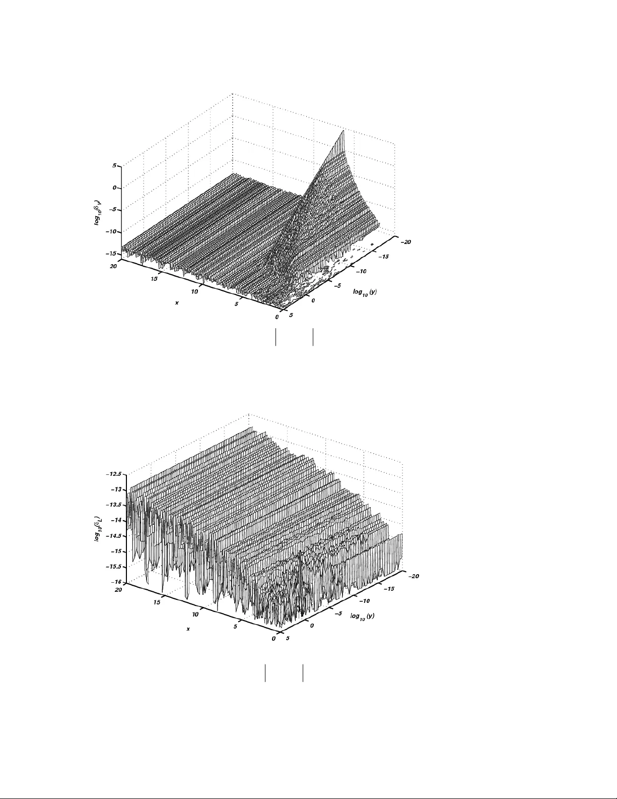
1 Algorithm 916: computing the Faddeyeva and Voigt functions MOFREH R. ZAGHLOUL, United Arab Emirates University 1 AHMED N. ALI, United Arab Emirates University We present a MATLAB function for the numeric al evaluatio n of the Faddeyeva function w ( z ). The function is based on a newly develo ped accurate algorithm . In addition to its higher accuracy, the software provides a flexible accuracy vs efficiency trade-off through a controlling parameter that m ay be used to reduce accuracy and computational time and vice versa. Verification of the flexibility, reliability and superi or accuracy of the algorithm is provided through comparison with standard algorithm s available in other libraries and software packages. Categories and Subject Descriptors: G.1.0 [ Numerical Analysis ] : General-Computer Arithmetic; Numerical Algorithm s; Multiple precision arithm etic; G.1.2 [ Numerical Analysis ] : Approximation-Special Func tions Approximations; G.4 [ Mathematical Software ]: Algorithm design and analysis; efficiency General Terms: Algorithms Additional Key Words and Phrases: Functi on evaluation, accuracy, Matlab, Faddeyeva function Author’s addresses: M. Zaghloul and A. Ali, Department of Physics, College of Sciences, United Arab Emirates University, Al-Ain, 17551, UAE. 2 1. INTRODUCTION The value and significance of the scaled complem entary error function for complex variables, also known as the Faddeyeva function or the pl asma dispersion function, is well recognized in the literat ure for its applications in several fields of physics [Armstrong 1967; Gautschi 1967; 1970; Hui et al. 1978; Humlí č ek 1982; Dominguez et al. 1987; Poppe et al. 1990; Le ther et al. 1991; Schreier 1992; Shippony et al. 1993; Weideman 1994; Wells 1999; Luqu e et al. 2005; Letchworth et al. 2007; Abrarov et al. 2010] . Plasma spectroscopy, nuclear physics, ra diative heat tran sfer, and nuclear magnetic resonance are a few examples of th e fields for which efficient and accurate evaluation of this function is required. Some of these appli cations require a sm all number of evaluations of the function where accuracy is m ore important than the computational time while other applications require enorm ous numbers of function evaluations, which imposes tight restr ictions on the com putational time. Accordingly, computational accuracy and computational tim e ar e issues of interest that should be critically add ressed and investigated in developing any successf ul algorithm for the computation of this function. Motivated by its practical importance and a lack of closed form expressions for the calculation of the Faddeyeva f unction, numerical evaluation of the function has been the focus of research over many decades [Armstrong 1967; Gautschi 1967; 1970; Hui et al. 1978; Humlí č ek 1982; Dominguez et al. 1987; Poppe et al. 1990; Lether et al. 1991; Schreier 1992; Shippony et al. 1993; Weidem an 1994; Wells 1999; Luque et al. 2005; Letchworth et al. 2007; Abra rov et al. 2010; Zaghloul 2007] . As a result, a wide variety of algorithms for the calculation of this func tion have been developed and presented in the literature. However, as it is shown in this study, mo st of these algorithms lose accuracy in some regions of the computational domain. We introduce a n ew algorithm for the calculation of th e Faddeyeva function which provides flexibility, reliability and supe rior accu racy. In section 2 we present the definition of the function and briefly summari ze some relevant fundamental m athematical relations. Then, in section 3, we establish the analytical basis of the algorithm while numerical analysis and computational deta ils are discussed in section 4. A short description of the Matla b function is given in section 5. Verification of the algorithm and comparisons with other com petitive codes in the lite rature are provided in section 6. 2. DEFINITION AND FUNDAMEN TAL MATHEMATI CAL RELATION S For a complex variable z=x+iy , the Faddeyeva (plasma dispersion) function, w ( z ), the real Voigt function, V ( x,y ) , the imaginary Voigt function, L ( x,y ), the complex error function, erf( z ), the imaginary error function, erfi( z ) and the Dawson’s integral F ( z ) are all closely related to each other. One can summarize these relations as () 0 y for y x, L i y x, V z F π i 2 e z i e iz e iz e iz e z 2 2 2 2 2 z z z z z > + = + = + = + = − = − − = − − − − − ) ( ) ( )) erfi( (1 )) erf( (1 ) erfc( )) erf( (1 ) ( w (1) 3 In the above relations, 1 i − = , erfc( z ) is the complementary error function, erfi( z ) is the imaginary error function which is related to th e erro r function by erfi( z ) = - i erf( iz ). As can be seen from the last line in (1), the real and im aginary Voigt functions are just the real and imaginary parts of the Faddeyeva function for y>0 , respectively. The evaluation of all of these functions can, therefore, be performed th rough the error function. The error function of a complex variable z can be regarded a s a line integral in the complex plane given by ∫ − = z t dt e z 0 2 2 ) ( erf π (2) Different paths can be taken to perform this line integral in the complex plane. For example, one may choose a linear path betwee n the initial point (origin) and the final point z which gives an expression for the complex error function of the form ∫ − = 1 0 2 2 2 ) ( erf dt e z z t z π (3) An alternative path can be followed through the line segments [0, 0 → iy ] and [0 → x, iy ] which gives, for the complex error function the expression,         − + = ∫ ∫ ∫ − − x t y y t x t y dt yt e e dt e i dt yt e e z 0 0 0 ) 2 sin( 2 2 ) 2 cos( 2 ) ( erf 2 2 2 2 2 π π π (4) In addition to the above paths, another simple and useful path from th e initial to the final points can be taken thro ugh the line segments [0 → x, iy =0] and [ x , 0 → iy ] which results in ∫ ∫ ∫ − − − + + = y t x y t x x t dt xt e e i dt xt e e dt e z 0 0 0 ) 2 cos( 2 ) 2 sin( 2 2 ) ( erf 2 2 2 2 2 π π π (5) The first term on the right hand side of (5) is the definition of the error function of the real variable x . Equation (5) is the basis of the present algorithm for the calculation of the Faddeyeva function as shown below. For some limiting value s of the parameters x and y , analy tical formulae do exist for the real and imaginary pa rts of the Faddeyeva function () [] () [] 2 ) 0 , ( ) ( ) 1 ( ) ( ) ( ) 1 ( ) ( 0 ) , 0 ( ) ( erfcx ) , 0 ( 2 2 2 2 2 2 2 2 x e y x V y x x y x L y x y y x V y x L y y x V − → → ± + → ∞ → + + → ∞ → + → → → → π π (6) where ) ( erfc ) ( erfcx 2 y e y y = is the scaled complementary erro r function of the real argument y . When y → 0 , the imaginary p art of the Faddeyeva function cannot be expressed as simply, however, it can be e xpressed in terms of Dawson’s integral of x (the real part of z ) where ) ( 2 ) 0 , ( x F y x L π → → ± (7) 4 and F ( x ) has well reporte d asymptotic expressions f or limiting values of x [Armstrong 1967] . Following Salzer 1951 [Salzer 1951] , we can write 1 ) ) 2 ( cosh 2 1 ( 2 2 2 2 1 ≤ ± + ≅ ∑ ∞ = − a e E ant e a e t n n a t π (8) where the relative error ∑ ∞ = − = 1 / ) / 2 cos( 2 2 2 2 n a n a t n e E π π is of the order of 2 2 / 2 ~ a e E π − . Table 1 presents some representati ve values of the relative erro r E corresponding to some values of the parameter a . Table 1: Relative error, E , of the representation of 2 t e given by Eq. (8) as a function of the parameter a . a 1.0 0.9 0. 8 0.7 0.6 0.5 0.4 0.36 E 1.03 × 10 -4 1.02 × 10 -5 4.01 × 10 -7 3.58 × 10 -9 2.48 × 10 -12 1.43 × 10 -17 3.25 × 10 -27 1.69 × 10 -33 3- ANALYTICAL BASI S OF THE ALGORITHM Replacing 2 t e in (5) by its representation given in (8), we get, for the real and imaginary parts of erf( z ), the following expressions [] ) 2 ( sin ) 2 ( sinh ) 2 ( cos ) 2 ( cosh 4 4 8 )) 2 ( cos 1 ( ) erf( )] [erf( Re 1 2 2 2 2 2 2 2 y x y n a n a y x y n a x x x n a e e π a xy e x π a x z n n a x x + − + × + − + = ∑ ∞ = − − − (9) [] ) 2 ( cos ) 2 ( sinh ) 2 ( sin ) 2 ( cosh 4 4 8 ) 2 ( sin ) 4 ( 4 )] [erf( Im 1 2 2 2 1 2 2 2 2 y x y n a n a y x y n a x x n a e e π a y x x e π a z n n a x x + + × + = ∑ ∞ = − − − − (10) The error in the expressions in (9) and (10) for the real and imaginary parts of the complex error function is controllable through the parameter a as indicated in Table 1. Both expressions, however, reduce to the formulae given by Salzer [Salzer 1951] and Abramowitz and Stegun [Abramowitz et al. 1972] with a rela tive error less than the floating point relative accuracy, ε , on a 16 digit computati onal platform, by setting a equal to 1/2 . An expression for the Faddeyeva function, ) ( erfc )] ( Im[ )] ( Re[ ) ( 2 iz e z i z z z − = + = − w w w , can be obtained by substituting (9) and (10) into (1). The resulting expression s for the real and imaginary parts of the Faddeyeva function are then given by 5 )] 2 ( cos ) 2 ( cosh [ 4 4 8 ] ) ( ) ( sin [ ) ( sin 2 ) 2 ( cos ) ( erfcx )] ( [ Re 1 2 2 2 2 2 2 2 2 y x x n a y n a e e π y a xy xy e π xy x a xy y e z n n a x x x − + + + = ∑ ∞ = − − − − w (11) )] 2 ( sinh ) 2 ( sin [ 4 4 8 ] ) 2 ( ) 2 ( sin [ 2 ) 2 ( sin ) ( erfcx )] ( [ Im 1 2 2 2 2 2 2 2 2 x n a n a xy y y n a e e π a xy xy e π x a xy y e z n n a x x x + + + + − = ∑ ∞ = − − − − w (12) Some comments on the above expressions may be useful at this stage 1- The series in (11) and (12) have an infinite number of terms and need to be truncated for practical use. The effect of such a truncation on the accuracy of the computations is predictable and can be controlled for a c onverging series, 2- While the exponential factors in the se ries are decaying with the index, n , they are multiplied by growing hyperbolic functi ons and one cannot directly determ ine where to truncate the infinite sum s for practical use, 3- There is a limitation on the evaluation of th e hyperbolic functions (related to the largest positive floa ting point number, R max , available on the computational platform). Since the argument of these hyperbolic functions is (2anx) , this will impose a strict restriction on the number of ter ms to be included in the sums for a given value of x with possible catastrophic consequences on both accuracy and reliability, 4- In writing the above expressions, the s caled complem entary error function of a real variable is used to reduce rounding error associat ed with the term (1-erf( y )), however, special care is needed for the evaluation of the erfcx( y ) function to avoid overflow problems illustrated in [Zaghloul 2007] . At present, m any software packages have well-behaved algorithms for computing the scaled complementary error function of a real variable, erfcx, and algorithms for accurate an d efficient computation of this function are available in the literature, 5- The evaluation of the quantity exp( -x 2 ) common to all of the above terms, can suffer underflow problems for large values of x . These problems can be avoided by combining this quantity with other large quantities wherever possible. To overcome the above-stated concerns and rest rictions, the expressions in (11) and (12) are rewritten in the form s       + + − + + = − − 3 2 1 2 2 ) 2 cos( 2 ] ) ( ) sin( [ ) sin( 2 ) 2 cos( ) ( erfcx )] ( [ Re 2 2 Σ Σ Σ π π y y xy y a xy xy e xy x a xy y e z x x w (13) and 6       + − + + − = − − 5 4 1 2 1 2 1 ) 2 sin( 2 )] 2 /( ) 2 [sin( 2 ) 2 sin( ) ( erfcx )] ( [ Im 2 2 Σ Σ Σ π π xy y a xy xy e x a xy y e z x x w (14) where ) ( 1 2 2 2 1 2 2 2 1 x n a n e y n a + − ∞ = ∑         + = Σ (15) 2 ) ( 1 2 2 2 2 1 x n a n e y n a + − ∞ = ∑         + = Σ (16) 2 ) ( 1 2 2 2 3 1 x n a n e y n a − − ∞ = ∑         + = Σ (17) 2 ) ( 1 2 2 2 4 x n a n e y n a an + − ∞ = ∑         + = Σ (18) 2 ) ( 1 2 2 2 5 x n a n e y n a n a − − ∞ = ∑         + = Σ (19) The convergence of the series (15)-(19) can be verifi ed by applying the simple ratio-test [Boas 2006] . In addition, in all of the above ex pressions (15)-(19), th e pre-exponential factors (fractions in bracke ts) of the argum ents of the summ ations assume values less than 1 for n> 1/ a . For a= 1/2 (which is suffi cient to express 2 t e by the expression given in (8) to machine accuracy on a 16-digit comput ational platform, see Table 1) the pre- exponential factors will alwa ys assume values less th an or equal to one for n ≥ 2 . For values of n ≥ 2, the terms in the series Σ 1 , Σ 2 and Σ 4 decrease monotonically with n while for relatively large va lues of x the term s Σ 3 and Σ 5 increase with n from one to a certain limit when they st art decaying monotonically with n . The fact that all exponential factors in the above summati ons eventually decay with increasing n provide s us with the possibility of obtaining a truncated series of practical use and computational efficiency as shown in the next section. It is understood, ho wever, that all of the above summations are to be performed using a sing le loop for computati onal efficiency. The loop specifications can be dete rmined once a cutoff scheme for the series in (15)-(19) is established. Moreover the comput ation of the exponentials in these series can be reduced to the computation of a single exponential and products using a single computational loop. This reduces the dependence on using the intrinsic function to calculate these exponentials within the loop and can save a significant amount of computational time. As the real part of the Fa ddeyeva function is even in x and its imaginary part is odd in x , we need only consider the right half of the complex plane ( x ≥ 0) since the even/odd properties of the real and imaginary pa rts of the function can be used to find the corresponding values in the le ft half of the plane. In addition, the values of ) ( z w in the lower half of the com plex plan e can be obtained from values in the upper half using the relationship ) ( 2 ) ( 2 z e z z w w − = − − (20) 7 which is equivalent to the sym metry relations ) , ( ) 2 sin( 2 ) , ( ) , ( ) 2 cos( 2 ) , ( 2 2 2 2 y x L xy e y x L y x V xy e y x V y x y x − − − − = − − − = + − + − (20’) Thus we do not lose generali ty by considering the evaluation of the function in just the first quadrant, however, we note that (20) re quires the subtraction of two values which leads to a loss of accuracy in the lower half. The practical usefulness of the calculation of the partial derivatives of the real and imaginary parts of the Faddeyeva functi on has been pointed out by many authors [10,13,15]. Once the Faddeyeva function has be en calculated accurately one can calculate these partial derivatives with relati ve sim plicity using the expression s )] , ( ) , ( [ 2 )] ( [ Re 2 ) , ( y x V x y x L y z z x y x V − = − = ∂ ∂ w (21) π π 2 )] , ( ) , ( [ 2 2 )] ( [ Im 2 ) , ( − + = − = ∂ ∂ y x V y y x L x z z y y x V w (22) in conjunction with the relations y y x V x y x L x y x V y y x L ∂ ∂ − = ∂ ∂ ∂ ∂ = ∂ ∂ ) , ( ) , ( & ) , ( ) , ( (23) Schreier [Schreier 1992] reports numerical problems that can arise when subtracting two numbers of approximately equal m agnitudes (when 0 ~ x V ∂ ∂ ). Letchworth and Benner [Letchworth et al. 2007] use a special algorithm to calcul ate these partial derivative (to accuracy <0.5%) but this increases th e com putational time by about 70%. 4- NUMERICAL ANALYSIS AND MACHINE LIMI TATIONS 4.1. High Accuracy Computations Due to the finite number of decimal digits available to store a real number in floating-point arithmetic, there are machine lim itations on the evaluation of the above summations. The floating-poi nt relative accuracy, ε , and the smallest positive floating- point number, R min , in the used computational platform impose restrictions on the accuracy and cause practical machine-truncatio n of the sums. At any stage durin g the computation of the sums, the new accu mulated sum after adding the term α n+1 of the series can be written as () ) ( 1 1 1 n n n n n ∆ Σ α Σ Σ + × = + = + + , (24) where n n n Σ α ∆ 1 ) ( + = . (24) implies that the sum of n+ 1 terms will not differ from the sum of n terms (i.e. the series will be effectively m achine-truncated) if the term n n n Σ α ∆ 1 ) ( + = becomes less than the floating-point relative accuracy, ε , or if α n+1 < R min . For computational efficiency (shorter computational time) we n eed to spe cify these in ternally truncated terms and exclude them fro m the computational loop. Starting with the sum Σ 1 and considering the possibili ty of machine-tru ncation of the sum due to the underflow of the terms α n+1 , a simple safe estim ation for the last value 8 of the index n to be included in the evaluation of the sum, 1 Σ cut n , can be derived based on the underflow of the exponential factors only (since the pre-exponential factor is already less than unity) 2 ) ln( 1 1 min , x R a n min R cut − − ≈ Σ (25) It is implicitly understood that (25) imp lies rounding to the nearest integer towards infinity. Sim ilarly, the terms of the sum s, Σ 2 and Σ 4 , have the same exponential dependence, while both of the pr e-exponential factors will have values less than or equal to unity for a / 1 n ≥ . In such a case, the term α n+1 in both sums will reach values < R min if the exponential factor becomes ≤ R min which gives [] x R a n min R cut − − ≈ ) ln( 1 4 2 min , , Σ Σ (26) Both (25) and (26) indicate that, for ) ln( min R x − ≥ , no terms from the arguments of the sums Σ 1 , Σ 2 and Σ 4 will be effective in the com putations and that the values of these sums will be effectively trunca ted. We note, however, that machine- truncation of these sums due to the R min limitation would also imply m achine-truncation due to machine accuracy (i.e, ∆ ( n ) ≤ε ) as seen in (24). For computational efficiency, this later condition may be used to break the computational loop as additional cycles of the computations or additional terms of the series will not chang e the values of the sum s. Furthermore, we can also m ake the computations of the sums Σ 3 and Σ 5 very efficient. As pointed out above, the values of the terms of these two series grow initially with n up to a certain value (peak) a nd then decay continuously as n increases. Simple investigation of these two sums shows that this peak is in the vicinity of n=x/a . Accordingly, if one starts cal culating these sums from around n=x/a and proceeds in both directions, the values of the terms will de crease until they get machine-trun cated. For each value of the index n used in the calculation of the term s of the sums Σ 1 , Σ 2 and Σ 4 we can add to each of the sum s Σ 3 and Σ 5 two terms by marching one step in each direction. The sums are truncated when the sum of the newly added two term s relative to the value of the previously accumulated sum becomes less than the machine accuracy . Handling the computation of the sums, Σ 3 and Σ 5 this way leads to a significant saving in execution time by dramatically reducing the number of terms requiring evaluation which, in turn, leads to a smaller number of loop cy cles. The asymptotic expression in the first line of (6) is used for values of x ½, the expansion in (8) becomes less accurate an d its accuracy will be governed by the corresponding value of the relative error, E, as shown in Table 1. It is not necessary, therefore, to keep the s trict condition for truncating the sum s, i.e., ∆ ( n ) < ε since the accuracy of the computations will be gove rned principally by the relative erro r E . Recalling that the relation between a and E can be written as E ~2 e − π 2 / a 2 it seems more appropriate to choose E (named tiny in the code) instead of ε to test for the convergence of the sums. That way we can reduce the number of terms included in the sum s by excluding terms that will not effectivel y enhance the accuracy and thus achieve 9 reasonable acceleration of the computations and reduce the com putational time. Noting that, changing the value of a changes E ( tiny ) and vice versa, we could choose either a or tiny as the free parameter for controlling the accuracy and efficiency of the computations. This free parameter will be used as an argum ent of the function. W e have chosen to use tiny and we calculate a internally from th e above relation as tin y gives a better indication of the accuracy of the computations. This allows flexibility for accuracy vs e fficiency trade-offs while maintaining the ability to run the code for high accu racy. 4.3. Calculation of the Exponentials and Other Numerical Considerations The central part of the present algorith m depends on the evaluation of the sum s (15)-(19) which all have exponential terms. The evaluation of intrinsi c functions like the exponential function is known to be slower th an other simple mathematical operations such as multiplication and/or division. A na ïve computation of thes e sum s would require three exponential evaluations per computati onal loop. This would be computationally expensive. However, we may reduce this to just one exponential evaluation in each cycle of the loop. For the case of ) ln( min R x − < we have some flexibility in evaluating the term 2 x e − either separately or by com bining it with other term s. In such a case one can write all of the exponentials in (1 5)-(19) in terms of the exponential 2 2 n a e − where 2 2 2 2 2 2 ) ( x n a x n a e e e − − + − × = (27) ∏ − − − + − × × = n ax x n a x n a e e e e 1 2 ) ( 2 2 2 2 (28) ∏ × × = − − − − n ax x n a x n a e e e e 1 2 ) ( 2 2 2 2 (29) In the above expressions 2 x e − , ax e 2 − and ax e 2 are calculated once outsi de the loop, for each value of x, and the products are simply perfor m ed using multiplies inside the computational loop. For ) ln( min R x − ≥ only Σ 3 and Σ 5 (which have the same exponential factor) contribute to the calculation of the real and im aginary parts of the Faddeyeva function. However, due to the natu re of the com putation of these terms, the exponential factor needs to be computed twice; once for the step to the right of n 0 = ceil( x/a ) and once on the left wing where “ceil” i ndicates rounding to th e nearest integer towards infinity. The indices for the se two factors are related to the loo p index, n , by n 3- plus = n 0 + ( n- 1) and n 3-minus = n 0 - n if n 3-minus ≥ 1, respectively. When n 3-minus <1, only the term on the right wing is included. The exponential factors for the terms on the left and right wings are related by ∏ − − − + − − − − × × = − − n a ax n a n a ax a x n a x n a e e e e plus 3 minus 1 ) 2 4 4 ( ) 2 2 ( ) ( ) ( 2 0 2 0 2 2 2 2 3 (30) Clearly the second exponential factor on the right hand side of (30) and the argument of the product may be calculated once out side the loop, for each value of x , thus reducing the number of exponential function evaluations to only one per cycle. The product can be evaluated using just multiplies inside the loop, thus reduc ing the computational time. 10 A few more important comput ational points are related to the calculatio n of the imaginary part of the Faddeyeva functi on using (14). Firstly, for values of x<<1 , the two sums Σ 4 and Σ 5 become very close to each other a nd the subtraction of these two sums could significantly affect the accuracy in regions of the computational dom ain where these two terms are the dominant term s in calculating the imaginary part of the Faddeyeva function. However, this problem can be simply overcom e by expressing the sum of these two terms (for x<< 1) in its original form as in (12), i.e. in term s of sinh(2 anx ). The first three terms in the series expansion of sinh( x ) will be sufficient to express sinh( x ) to the machine accuracy for x ≤ 10 -2 and since 2 an is usually <20 in the present computations then this is satisfactorily f or x ≤ 5×10 -4 . The second important point in the calculation of the imaginary part of the Faddeyeva function using (14) is related to the calculation of the sum of the first three terms on the right hand side of the equation, for ) ln( min R x − < , which can be written safely in the f orm                   + + + − ∑ ∞ = − − 1 2 2 2 1 2 1 ) ( ) ( sin 2 2 2 n n a x y n a e y a y 2xy e π erfcx (31) The terms in the curly brackets are only dependent on y and for y ≥ 5 we have found that this sum is zero to machine accuracy. Using this prevents rounding errors affecting the accuracy of computations. Note that for very sm all values of x the result of the whole expression (31) is O( yx) while the total of - Σ 4 + Σ 5 is O( x), the significance of rounding errors is thus clear fo r small values of x and relatively large values of y . 5. THE MATLAB FUNCTI ON FADDEYEVA.M The function Faddeyeva( z ,tiny ) returns, in general, an array of complex values for the Faddeyeva function of th e same size as the input a rray for the complex variable z . The input z is usually an array (with one or two dimens ions) but can be a sin gle scalar as well. When z contains only imaginary values z= i y, the function returns the real values calculated from the MATLAB built-in function “erfcx( y )”. The function is set for the calculation for the whole complex dom ain . However, for negative values of y and exp( y 2 - x 2 ) greater than the largest floating point number in the computational platform, Faddeyeva cannot calculate the Faddeyeva function due to inescapable overflow problems. The function checks for acceptable va lues and issues an error message for any points outside this domain. The value of the scalar free parameter “ tiny” can be chosen by the user within the range tiny min ≤ tiny ≤ 10 -4 to control the accuracy and comp utational tim e. The value of tiny min is a value close to but less than the floating-point relativ e accuracy, ε . For example, for a 16 digit computational platform, tiny min can be taken roughly to be ~1.43×10 -17 (the value of E corresponding to a =1/2 in Table 1) while for a 32-digit computational platform tiny min can be taken to be roughly 10 -33 . Th e maxi mum va lue o f tiny =10 -4 corresponds to a =1 (the maximum value for a for which the expansion in (8) can be used). Increasing the value of tiny within its above mentioned range will d ecrease the computational time at the exp ense of the computational accuracy and vice versa. Choosing a value of tiny < tiny min will just increase th e run time without any improvement in the accu racy of computations which will then be governed solely by the 11 machine characteristics. Values of tiny < tiny min or tiny>10 -4 result in tiny being reset to tiny min or 10 -4 respectively; a warning m essage is returned in both cases. It is to be noted that tiny< ε is used only for the calculation of the corresponding value of the parameter a and not for the truncation of the sums since the calculations cannot be claimed to be performed for relati ve accuracy less than the machine accuracy epsilon, ε , in any case. Accordingly, for the tr uncation of the sums, the maximum of tiny and ε is used. 6. ALGORITHM VERIFICAT ION AND EFFICIENCY 6.1. High Accuracy Com putations Three different independent computational techniques are used to investigate the accuracy of the present algorithm 1- Mathematica  [Wolfram Research, Inc. 2008] provides the im aginary error function erfi( z ) as a special function which can be ev aluated and then used in conjunction with the relation given in (1) ; that is ) ) ( erfi 1 ( ) ( 2 z i e z z + = − w , to calculate the Faddeyeva function [Zaghloul 2008] . The arbitrary-precision arithmetic used in Mathematica  allows us to obtain highly accurate valu es for the function erfi(z) although these calculations are very expensiv e computationally. This is only generally suitable for applications where the speed of arithmetic is n ot a restrictive factor, or where precise results for a small number of evaluations ar e required. W e can, however, generate highly accurate values of the function erfi( z ) using Mathematica  by using large num bers of digits of precision, 2- the simple proper integral given in reference [Zaghloul 2007] can be used to calculate the real Voigt f unction (real part of the Faddeyeva function), and 3- the Algorithm 680 [Poppe et al. 1990] , which is widely used in the literature and is implemented in m any software packages and libraries, calculates the Faddeyeva function to a claimed accuracy of 14 significant digits. The relatively long comput ational time associated w ith the first two methods makes them inefficient for use in applic ations requiring a large number of function evaluations. For this reason, Algorithm 680 is regarded as the com petitive highly accurate algorithm due to its computationa l speed and claim ed accuracy. Table 2 presents sample results calculat ed using these thre e methods with the results from the present algorithm. The values of the complex variable z used in the computations in this tab le have been selected to allow som e conclusions to be drawn in addition to establishing confidence and reliability in th e present code. The value of the relative error in the ca lculation of the Faddeye va function proposed here is given in Table 3 and compared with the other a pproaches, taking the values of w calculated using the function erfi( z ) from Mathematica  with high num ber of digits of accuracy as reference values. Looking closer into the values given in these two tables we conclude that; a) com pared to calculating the Fa ddeyeva function using erfi( z ) from Mathematica  , the pres ent algorithm is m ore reliable since we failed to calculate erfi( z ) using Mathematica  for values of x >3.9 × 10 4 and y >2.8 × 10 4 while the 12 present algorithm does not suffer such a lim itation. Note that for this dom ain Mathematica  cannot be used as reference, and therefore, no com parison was performed for this range in Table 3. b) for the whole domain of computations, th e present algorithm shows very high accuracy as shown in Table 3, while the Algorithm 680 suffers a catastrophic loss of accuracy in the vicinity of x =6.3 as well as for small values of y sig nified by bold-face numbers in Tables 2 and 3. The relative error for the real part of the Faddeyeva function from Algor ithm 680 in this region of the first quadrant goes up to 100%. It has to be noted that x =6.3 is one of the built -in values in Algorithm 680. To investigate the effectiveness of the pr esent algorithm compared to Algorithm 680, we calculated the Faddeyeva function using both algorithms for 2,840,710 points of the complex variable z distributed over the upper half of the complex plane using the grid y=logspace ( -20, 4, 71 ) and x=linspace ( -200, 200, 40001 ) where y=logspace ( -20, 4, 71 ) generates a row vector of 71 logarithm i cally equally spaced po ints between 10 - 20 and 10 4 and x=linspace ( -200, 200, 40001 ) generates a row vector of 40001 linearly equally spaced points between -200 and 200. Using Matlab 7.9.0.529 (R2009b) , the computational time taken by the present al gorithm was found to be <8.0% of that taken by Algorithm 680, which represen ts a significant time saving. Figures (1-a) and (1-b) show su rface pl ots of the ab solute relative error ref ref V V V V δ / − = and ref ref L L L L δ / − = in the results obtained fr om the present algo rithm using results from Algorithm 680, which is ava ilable in Matlab, as reference values. As can be clearly seen from these figures, the resu lts from the present algorithm show high agreement (around 13 significant d igits) ov er the chosen computational dom ain except for the region in the vici nity of x =6.3 and small values of y where Algorithm 680 badly loses its accuracy as indicated above. The above findings provide the necessary verification and confirm the high accuracy as well as the reliability of the present algorithm. 13 Figure 1-a Absolute relative error ref ref V V V V δ / − = in the calculations of the real part of the Faddeyeva function from the pres ent algorithm using the re sults from Algorithm 680 as reference values. Figure 1-b Absolute relative error ref ref L L L L δ / − = in the calculations of th e imaginary part of the Faddeyeva function from the pres ent algorithm using the re sults from Algorithm 680 as reference values. 14 6.2. Efficient Computations with Lower Accuracies Table 4 below shows values of the free variable tiny used in the calling argument of our Matlab function and the corresponding relative accuracy ref ref V V V V δ / ) ( − = and ref ref L L L L δ / ) ( − = in the calculations, usin g values ca lculated with the highest accuracy obtainable from the present algorithm as re ference values. The need to quantify the efficiency improvements obtainable when usin g the accuracy vs efficiency trade-off capability of the present algorithm is th e reason of using the highest accuracy computations from the present algorithm as reference values. The run times required to calculate the function for 2,840,710 points generated using the grid y=logspace ( -20, 4, 71 ) and x=linspace ( -200, 200, 40001 ) relative to the run tim e required to perform the same comp utations using the highest accuracy com putations from the present algorithm are also included in the table. As can be seen from the table, run ning the present algorithm at lower accuracy im proves the effici ency of the computations and decreases the computational time by up to 45 %. Comp ared to other efficient and low-accu racy algorithms in the literature [Hui et al. 1978; Hum lí č ek 1982; Poppe et al. 1990; Lether et al. 1991; Shippony et al . 1993; Weideman 1994] , the present algorithm seems to be mo re reliable even at low-accuracy . In addition, other algorithms fail in some regions of the computational domain, particularly near the real axis (very sm all values of y ); for example, the Poppe and W ijers algorithm [Poppe et al. 1990] , known for its accuracy , fails in this region, returning resu lts for the real part of the Fadde yeva function that are several orders of magnitude aw ay from the correct values. Figure 2 shows a comparison betw een the ca lculations of the partial derivative x y x, V ∂ ∂ ) ( using the present algorithm (run at th e lowest accuracy) an d calculations from Algorithm 680, for y =10 -20 , in the region x =[6.1-6.5] . Here we see that the resu lts from the present algorithm (e ven when run at the lowest accuracy ) seem to be more accurate and more reliable than computations from Poppe and Wijers algorithm in this region, where the latter loses its accuracy and fails to produce the correct behavior of x y x, V ∂ ∂ ) ( . 15 Figure 2 ∂ V(x,y)/ ∂ x as calc ulated, f rom the pres ent algorith m ( tiny =10 -4 ) and from Poppe and Wijers algorithm, using ( 21), for y =10 -20 . Figure 3 shows a surface plot of the relative error ref ref V V V V δ )/ ( − = for the results obtained from Hui’s algorithm [Hui et al. 1978] using results from the present algorithm as reference v alues. We note that th e Matlab version of Hui’s algorithm (cerf.m [Hui et al. 1978] ) employed in this comparison, uses the p =5 rational approximation where p is the degree of nominator polynomial. As is clear from the plot, the relative errors in the results of Hui’s a lgorithm are very large f or small values of y and reach 14 order of magnitude for medium values of x when y =10 -20 . In addition to the large errors for medium values of x and small values of y , Hui’s algorithm produces negative values for the Vo igt function (real part of the Faddeyeva function) for example, for y =10 -5 and x =4. The Voigt function is positive over the whole first quadrant. 16 Figure 3 Absolute relative error, ref ref V V V V δ )/ ( − = , in the calculatio ns of the real part of the Faddeyeva fu nction from Hui’s al gorithm using results fro m the present algorithm ( tiny = tiny min ) as reference values. Figure 4 shows a comparison betw een the ca lculations of the partial derivative x y x, V ∂ ∂ ) ( using the present algorithm (run at th e lowest accuracy) an d calculations from Hui’s algorithm, using (21), for y =10 -20 , in the region x =[7,15] . As we see from the figure, calculations from the present algo rithm seem to be more accurate and m ore reliable than Hui’s algorithm which fails to produce the co rrect behavior (negative x y x, V ∂ ∂ ) ( ) or the correct order of magnitude of x y x, V ∂ ∂ ) ( in this region of the computational domain. We note that the error contours given in [Hui et al. 1978] were p resented either for the modulus of the complex erro r function or for the absolute value of the Voigt function V ( x,y ). That was, probably, the reason w hy such failures were not clear from their paper. Although Hui’s algorithm takes about 10% of the computational tim e taken by the present algorithm (for tiny =10 -4 ) and about 5% of the computational time taken by the present algorithm for the highest-accuracy com putations, th e fact that it fails to produce the correct values or correct signs of the function or even its correct behavior, in this region of the computational dom ain, poses important questio ns about its reliability. 17 Figure 4 ∂ V(x,y)/ ∂ x as calculated, from the present algorithm ( tiny =10 -4 ) and from Hui’s al gorithm, using (21), fo r y =10 -20 . Humlí č ek [Humlí č ek 1982] reported that any rational approximation suffers inevitable failure ne ar the r eal axis and he attempted to overcom e this failure in his algorithm, w4. However, invest igating the results of H umlí č ek’s algorithm we found that it also suffers com plete failure ne ar the real axis in the v icinity of x =5.5. The results for y =10 -20 s h o w t h a t H u m l í č ek’s algorithm underestimates the real part of the Faddeyeva function by 8 orders of magnitude and by 3 orders of magnitude for y =10 -15 . Figure 5 shows a surface plot of the relati ve error in th e calculation of V ( x , y ) using Humlí č ek’s algorithm taking the results f rom the present algorithm as reference. Table 5 shows that the com putational time using the Hum lí č ek’s original code is almost three times that us ed by the pr esent algorithm (for the highest-accuracy computations). Even using a mo re efficient version of Humlí č ek’s code, m odified by the present authors, we note that th e computational time taken by Hum lí č ek’s algorithm is still longer than that taken by the pres ent algorithm (for the highest-accuracy computations). Figure 6, on the other hand, shows a co mparison between th e calculations of the partial derivative x y x, V ∂ ∂ ) ( using (21) from the present algorithm (run at the low est accuracy) and those calculations from Humlí č ek’s algo rithm, for y =10 -20 , in the region x =[5.4,6.4] . This shows that Hum lí č ek’s algorithm does not produ ce the correct behavior of x y x, V ∂ ∂ ) ( in this dom ain. 18 Figure 5 Absolute relative error, ref ref V V V V δ / ) ( − = , in the calculations of the real part of the Faddeyeva functi on from Huml í č ek’s algorithm using results from the present algorithm ( tiny = tiny min ) as reference values. Figure 6 ∂ V(x,y)/ ∂ x as calculated, from th e present algorithm ( tiny =10 -4 ) and from Humlí č ek’s algorithm, using ( 21), for y =10 -20 . 19 As with Hui’s a lgorithm, Weidem an’s algorithm [Weideman 1994] also produces negative values for the real part of the Faddeyeva functi on near the real axis. The negative values for the Voigt function calcu la ted from W eideman’s algorithm appear fo r all values of the param eter N (number of term s in the rational serie s) for y =10 -20 . A surface plot of the relative er ror in the calculati ons of the real part of the Faddeyeva function using Weideman’s al gorithm with N=256 taking th e results of the present algorithm as a reference is show n in Figure 7. The figure show s that the errors resulting from Weidem an’s algorithm are catastrophic for sm all values of y and that the com puted magnitude of V ( x , y ) is overestim ated by up to 6 orders of magnitude for y =10 -20 . The situation becom es even worse for sm aller values of N. Table 5 shows th at the run tim e of the present algorithm at highest accuracy is sho rter than the run time of Weidem an’s algorithm with N=256. Figure 7 Absolute relative error, ref ref V V V V δ / ) ( − = , in the calculations of the real part of the Faddeyeva fu nction from Weideman’s al gorithm, N= 256, using resul ts from the present algorithm ( tiny = tiny min ) as reference values. Figures (8-a) and (8-b) show com parisons between the calcu lations of the partial derivative x y x, V ∂ ∂ ) ( using the present algorithm (r un at the lowest accuracy) and Weideman’s algorithm with N=128 and N=32, respectively. The calculations show n in the figure are for the region x =[6,15] and y =10 -20 in Figure (8-a) and y =10 -10 in Figure (8- b) . From these figures, we see that Weidem an’s algorithm does not reproduce the correct behavior for x y x, V ∂ ∂ ) ( in the regions shown. 20 Figure 8-a ∂ V(x,y )/ ∂ x as calculated, from the present algorithm ( tiny =10 -4 ) and from Weideman’s algorithm with N=128, using (21), for y =10 -20 . Figure 8-b ∂ V(x,y )/ ∂ x as calculated, from the present algorithm ( tiny =10 -4 ) and from Weideman’s algorithm with N=32, using (21), for y =10 -20 . 21 Other competitive algorithm s in the literat ure also show loss of accuracy in some regions of the computational domain. For example, the algorithm by Shippony and Read [Shippony et al. 1993] exhibits the same failure in ca lculating the real part of the Faddeyeva function near the real axis. In part icular we detected the same loss of accuracy suffered by Poppe and Wijers algorithm for very small values of y near x =6.3. In addition, the Shippony and Read algor ithm produces negative values for V ( x,y ) and/or L ( x,y ) in several regions of the computational dom ain. Just for example we refer to the points at x =1.5 and y =1.5, 2.0, 2.5, 3.0, 3.5, 4.0, 5.0 etc. It has to be noted that these failures have been obtained even with the use of the correction provided by Shippony and Read in [Shippony et al. 2003] . The situation is no better with the Letchworth and Benner’s algorithm [Letchworth et al. 2007] where similar failures and loss of accuracy are obtained for very sm all values of y and values of x greater than but close to x =5.76. For x =5.76 and y =10 -20 Letchwoth and Benner’s algorithm returns, for the real part of Faddeyeva function the value V =1.783900323491466×10 -22 while the value returned from the pres ent algorithm is V =3.900779639194698×10 -15 and that returned from using the function erfi( z ) from Mathematica TM is 3.900779639194697×10 -15 . The algorithm in [Zaghloul 2007] returns 3.900779639194698×10 -15 . Figure 9 shows a similar comparison between the calculations of the partial derivative x y x, V ∂ ∂ ) ( using the present algorithm (with tiny =10 -4 ) and calculations from Letchworth and Benner algorithm, in (21), for y =10 -20 . The failure of Letchworth and Be nner’s algorithm for values of x greater than but close to x =5.76 can be easily recogni zed from the figure. It has to be emphasized here that these "com petitive codes" were (prob ably) not designed for such extreme values of y and the tests presented here are m ore a demonstration of the "superior accu racy" of our software even for extreme values. Figure 9 ∂ V(x,y)/ ∂ x as calc ulated, f rom the pres ent algorith m ( tiny =10 -4 ) and from L etchworth & Benner’s algorithm, using (21), for y =10 -20 . 22 7. CONCLUSIONS An algorithm accom panied by a computer code, in the form of a MATLAB TM function, for the numerical evaluation of the Faddeyeva function w (z) is presen ted. The algorithm is more accurate and avoids failures discovered in other com petitive published algorithms. In addition to its superior ac cur acy, the present algorithm and com puter code allow a flexible accuracy vs efficiency trade-off through controlling a free parameter tiny . By adjusting the value of this par ameter th e function can b e run with a lower accuracy and shorter computational time or high accur acy and longer computational time. Even when run at its lowest accur acy, the present algorithm avoi ds m ajor problems suffered by other competitive codes. For all lev els of accuracy the present code is safer and more reliable since it does not retu rn negative valu es for real and/or imaginary parts of the Faddeyeva function nor does it suffer from the loss of accuracy exhibited by som e of the other competitive codes. The present algo ri thm can, therefore, be safely used and implemented in personal and commercial libraries. 23 Table 2: Results from algorithms in the literature in com parison with resu lts from the present al gorithm for some sele cted valu es of z z Mathematica TM Algorithm 680 [Z aghloul 2007] Present algorithm x y V L V L V V L 6.3e-002 1.0e -020 9.96 0388660702 479e-001 7.09000872 6353683e-00 2 9.9603886607 02479e-001 7.0900 0872635368 5e-002 9.96038866 0702479e-00 1 9.96038866 0702479e-00 1 7.0900087263 53669e-00 2 6.3e-002 1.0e -014 9.96 0388660702 367e-001 7.09000872 6353558e-00 2 9.9603886607 02367e-001 7.0900 0872635356 0e-002 9.96038866 0702366e-00 1 9.96038866 0702366e-00 1 7.0900087263 53543e-00 2 6.3e-002 1.0e -012 9.96 0388660691 284e-001 7.09000872 6341133e-00 2 9.9603886606 91284e-001 7.0900 0872634113 5e-002 9.96038866 0691284e-00 1 9.96038866 0691284e-00 1 7.0900087263 41118e-00 2 6.3e-002 1.0e -010 9.96 0388659583 033e-001 7.09000872 5098674e-00 2 9.9603886595 83034e-001 7.0900 0872509867 6e-002 9.96038865 9583034e-00 1 9.96038865 9583033e-00 1 7.0900087250 98659e-00 2 6.3e-002 1.0e -006 9.96 0377466254 799e-001 7.08999617 6278113e-00 2 9.9603774662 54800e-001 7.0899 9617627811 3e-002 9.96037746 6254802e-00 1 9.96037746 6254801e-00 1 7.0899961762 78086e-00 2 6.3e-002 1.0e -002 9.84 9424862549 036e-001 6.96590965 7459020e-00 2 9.8494248625 49037e-001 6.9659 0965745902 1e-002 9.84942486 2549038e-00 1 9.84942486 2549039e-00 1 6.9659096574 59005e-00 2 6.3e-002 1.0e +001 5. 6138818328 23887e-002 3.502232 333332985e -004 5.61388183 2823888e-00 2 3.5022323333 32986e-004 5.613881 832823887e -002 5.613881 832823886e -002 3.502232 333332973e -004 6.3e-002 1.2e +001 4. 6852951492 11636e-002 2.442987 772965768e -004 4.68529514 9211637e-00 2 2.4429877729 65769e-004 4.685295 149211637e -002 4.685295 149211637e -002 2.442987 772965766e -004 6.3e-002 1.5e +001 3. 7528951614 91573e-002 1.569287 266610685e -004 3.75289516 1491574e-00 2 1.5692872666 10686e-004 3.752895 161491573e -002 3.752895 161491574e -002 1.569287 266610681e -004 6.3e-002 2.0e +002 2. 8209123773 24508e-003 8.885651 855627418e -007 2.82091237 7324509e-00 3 8.8856518556 27419e-007 2.820912 377324511e -003 2.820912 377324508e -003 8.885651 855627396e -007 6.3e-002 1.0e +005 Fails to evaluate erfi 5.64189583 5193230e-00 6 3.5543943758 16296e-012 5.6418 9583547532 4e-006 5.6418 9583519322 8e-006 3.554394375816285e -012 6.3e+000 1.0e -020 5.79246077 8844102e-01 8 9.07276596 8412736e-00 2 1.47893449 2449188e-02 2 9.07276596 8412733e-00 2 5.79231288 5394871e-01 8 $ 5.79246077 8844116e-01 8 9.07276596 8412679e-00 2 6.3e+000 1.0e -014 1.53685762 1303171e-01 6 9.07276596 8412736e-00 2 1.47893449 2449189e-01 6 9.07276596 8412733e-00 2 1.53685762 1303171e-01 6 1.53685762 1303163e-01 6 9.07276596 8412679e-00 2 6.3e+000 1.0e -012 1.47951372 3737762e-01 4 9.07276596 8412736e-00 2 1.47893449 2449189e-01 4 9.07276596 8412733e-00 2 1.47951372 3737762e-01 4 1.47951372 3737753e-01 4 9.07276596 8412679e-00 2 6.3e+000 1.0e -010 1.47894028 4762108e-01 2 9.07276596 8412736e-00 2 1.47893449 2449189e-01 2 9.07276596 8412733e-00 2 1.47894028 4762108e-01 2 1.47894028 4762099e-01 2 9.07276596 8412679e-00 2 6.3e+000 1.0e -006 1.47893449 3028413e-00 8 9.07276596 8412492e-00 2 1.47893449 2449148e-00 8 9.07276596 8412488e-00 2 1.47893449 3028413e-00 8 1.47893449 3028404e-00 8 9.07276596 8412433e-00 2 6.3e+000 1.0e -002 1.4789 3038913394 2e-004 9.0727415163 49275e-002 1.4789 30389133 851e-004 9.072741 516349273e -002 1.4789303891 33943e-004 1. 4789303891 33934e-004 9.072741516349 218e-002 6.3e+000 1.0e +001 4.04 0671157393 860e-002 2.52757727 7549421e-00 2 4.040671157393 860e-002 2.5275 7727754942 2e-002 4.04067115 7393859e-00 2 4.04067115 7393835e-00 2 2.5275772775 49405e-002 6.3e+000 1.2e +001 3.68 4277239564 821e-002 1.92380885 7910893e-00 2 3.684277239564 821e-002 1.9238 0885791089 2e-002 3.68427723 9564818e-00 2 3.68427723 9564798e-00 2 1.9238088579 10881e-002 6.3e+000 1.5e +001 3.19 4834330452 624e-002 1.33679711 4261604e-00 2 3.194834330452 625e-002 1.336797 11426160 5e-002 3.1948343304 52623e-002 3. 1948343304 52605e-002 1.3367971142 61596e-002 6.3e+000 2.0e +002 2.81 8116555672 224e-003 8.87684545 7496914e-00 5 2.818116555672 223e-003 8.876845 45749691 1e-005 2.8181162256 91620e-003 2. 8181165556 72206e-003 8.8768454574 96856e-005 6.3e+000 1.0e +005 Fails to evaluate erfi 5.64189581 2802784e-00 6 3.5543943617 10315e-010 5.6418 9581308487 9e-006 5.6418 9581280274 6e-006 3.554394361710292e -010 6.3e+002 1.0e -020 1.4214 9588258239 4e-026 8.9554 0149675710 4e-004 1.42 1495882582 395e-026 8.9554 0149675710 4e-004 1.42149051 0324405e-02 6 1.42149588 2582395e-02 6 8.95540149 6757105e-00 4 6.3e+002 1.0e -014 1.4214 9588258239 4e-020 8.9554 0149675710 4e-004 1.42 1495882582 395e-020 8.95540149 6757104e-00 4 1.42149051 0324405e-02 0 1.42149588 2582395e -020 8.95540149 6757105e-00 4 6.3e+002 1.0e -012 1.4214 9588258239 4e-018 8.9554 0149675710 4e-004 1.42 1495882582 395e-018 8.9554 0149675710 4e-004 1.42149051 0324405e-01 8 1.42149588 2582395e-01 8 8.9554014967 57105e-004 6.3e+002 1.0e -010 1.4214 9588258239 4e-016 8.9554 0149675710 4e-004 1.42149588258239 5e-016 8.95 5401496757 104e-004 1.421490 510324405e -016 1.421495 882582395e -016 8.95540149 6757105e -004 6.3e+002 1.0e -006 1.4214 9588258239 4e-012 8.9554 0149675710 4e-004 1.42149588258239 4e-012 8.955401 496757104e -004 1.421490 510324405e -012 1.421495 882582395e -012 8.95540149 6757105e -004 6.3e+002 1.0e -002 1.4214 9588222424 1e-008 8.9554 0149450075 3e-004 1.42 1495882224 242e-008 8.95540149 4500753e-00 4 1.42149050 9966257e-00 8 1.42149588 2224242e -008 8.95540149 4500755e-00 4 6.3e+002 1.0e +001 1.42 1137820009 847e-005 8.95 3145713915 760e-004 1. 4211378200 09848e-00 5 8.953145713915 762e-004 1.421132 452261351e -005 1.421137 820009847e -005 8.95314571 3915762e -004 6.3e+002 1.2e +001 1.70 5176395541 706e-005 8.95 2153529445 874e-004 1. 7051763955 41707e-00 5 8.952153529445876e -004 1.705169 95662271 1e-005 1.705176 39554170 7e-005 8.952153529445874e -004 6.3e+002 1.5e +001 2.13 1035743074 597e-005 8.95 0327582962 093e-004 2. 1310357430 74598e-00 5 8.950327582962 093e-004 2.131027 699897097e -005 2.131035 743074598e -005 8.95032758 2962094e -004 6.3e+002 2.0e +002 2.58 2702147491 469e-004 8.13549314 3556982e-00 4 2.5827021474 91469e-004 8.1354 93143556 982e-004 2.58269436 2772975e-00 4 2.58270214 7491469e-00 4 8.13549314 3556982e-00 4 6.3e+002 1.0e +005 Fails to evaluate erfi 5.64167191 7237129e-00 6 3.55425330750397 9e-008 5.64167191 7519157e-00 6 5.64167191 7237128e-00 6 3. 5542533075 03980e-008 1.0e+000 1.0e -020 3.6787 9441171442 3e-001 6.0715770584 13937e-001 3.6787 94411714 423e-001 6.071577 058413937e -001 3.6787944117 14423e-001 3. 6787944117 14423e-001 6.071577058413 938e-001 5.5e+000 1.0e -014 7.3073 8672952877 3e-014 1.0436743643 67812e-001 7.3082 45082486 227e-014 1.043674 364367812e -001 7.30738672 9528773e-01 4 ∗ 7.30738672 9528773e-01 4 1.043674364367 812e-001 3.9e+004 1.0e +000 Fails to evaluate erfi 3.70933322 6385424e-01 0 1.4466399573 39204e-005 3.7093 3322272730 4e-010 3.7093 3322638542 3e-010 1.446639957339204e -005 1.0e+000 2.8e +004 Fails to evaluate erfi 2.01496279 4529686e-00 5 7.1962956855 69928e-010 2.0149 6279581473 9e-005 2.0149 6279452968 6e-005 7.196295685569929e -010 * This is the correct value as calculated using (4) in [Zaghloul 2007] . The value given in Table 4 in the sa me reference is calculated us ing the asymptotic expression for y → 0 $ Calculated using the as ymptotic expression for y → 0 24 Table 3: Values of the relative errors ref ref V V V V δ / ) ( − = & ref ref L L L L δ )/ ( − = in calculating the Faddeyeva function by differe nt codes using values of the function calculated using erfi (z) from Mathematica  as reference v alues. z Algorithm 680 Zaghloul [2007] Present algorithm x y V L V V L Maxim um no. of series terms 6.3e-002 1. 0e-020 0 2.0e-016 0 0 2.0e-1 5 12 6.3e-002 1. 0e-014 0 2.0e-016 1.1e-016 1. 1e-016 2.1e-15 12 6.3e-002 1. 0e-012 0 2.0e-016 0 0 2.1e-1 5 12 6.3e-002 1. 0e-010 1.1e-016 2.0e-016 1.1e-0 16 0 2.1e-15 12 6.3e-002 1. 0e-006 0 0 2.2e-016 1.1e-0 16 3.7e-15 12 6.3e-002 1. 0e-002 1.1e-016 2.0e-016 2.3e-0 16 3.4e-016 2.2e-15 12 6.3e-002 1.0e+0 01 2.5e-016 1.6e-016 0 1.2e-016 3.6e-1 5 13 6.3e-002 1.2e+0 01 3.0e-016 2.2e-016 3.0e-016 3. 0e-016 8.9e-16 13 6.3e-002 1.5e+0 01 3.7e-016 6.9e-016 0 5.5e-016 2.6e-1 5 13 6.3e-002 2.0e+0 02 3.1e-016 1.2e-016 1.1e-015 0 2.4e-15 13 6.3e+000 1.0e- 020 1.0e-000 3.1e-016 2.6e-005 2. 4e-015 1.2e-016 13 6.3e+000 1.0e- 014 3.8e-002 3.1e-016 0 5.3e-015 1.2e-016 13 6.3e+000 1.0e- 012 3.9e-004 3.1e-016 0 6.2e-015 1.2e-016 13 6.3e+000 1.0e- 010 3.9e-006 1.5e-016 0 6.1e-015 1.2e-016 13 6.3e+000 1.0e- 006 3.9e-010 4.6e-016 0 6.0e-015 1.2e-016 13 6.3e+000 1.0e- 002 6.2e- 014 3.1e-016 7.3e-016 5.3e-0 15 2.4e-016 13 6.3e+000 1.0e+00 1 0 4.1e-016 3.4e- 016 6.2e-015 2.4e-016 13 6.3e+000 1.2e+00 1 0 5.4e-016 9.4e- 016 6.2e-015 0 13 6.3e+000 1.5e+00 1 2.2e-016 7.8e-016 4.3e-016 6.1e-015 1.2e-016 13 6.3e+000 2.0e+00 2 3.1e-016 3.1e-016 1.2e-007 6.3e-015 0 13 6.3e+002 1.0e- 020 6.1e- 016 0 3.8e-006 6. 1e-016 1.2e-016 13 6.3e+002 1.0e- 014 8.5e- 016 0 3.8e-006 8. 5e-016 1.2e-016 13 6.3e+002 1.0e- 012 6.8e- 016 0 3.8e-006 6. 8e-016 1.2e-016 13 6.3e+002 1.0e- 010 6.9e- 016 0 3.8e-006 6. 9e-016 1.2e-016 13 6.3e+002 1.0e- 006 0 0 3.8e- 006 5.7e-016 1.2e-016 13 6.3e+002 1.0e- 002 7.0e- 016 0 3.8e-006 7. 0e-016 2.4e-016 13 6.3e+002 1.0e+00 1 7.2e-016 2. 422e-01 6 3.8e-006 0 2.4e-016 13 6.3e+002 1.2e+00 1 6.0e-016 2. 422e-01 6 3.8e-006 6. 0e-016 0 13 6.3e+002 1.5e+00 1 4.8e-016 0 3.8e-006 4.8e- 016 1.2e-016 13 6.3e+002 2.0e+00 2 0 0 3.0e-0 06 0 0 13 1.0e+000 1.0e- 020 0 0 0 0 1.8e- 016 13 5.5e+000 1.0e- 014 1.2e-004 0 0 0 0 13 25 Table 4: Accuracy vs efficiency trade-off of the present algor ithm (computations are perform ed on an array of 2,840,710 point s generated using the grid y=logspace ( -20, 4, 71 ) and x=linspace ( - 200, 200, 40001 ) using Matlab 7.9.0.529 (R2009b) ). tiny min min / tiny tiny tiny max V, V V V − = δ min min / tiny tiny tiny max L, L L L − = δ Run time (s) 0.06447× ε 1.0e-15 1.0e-14 1.0e-12 1.0e-10 1.0e-09 1.0e-08 1.0e-07 1.0e-06 1.0e-05 1.0e-04 0 4.6e-013 4.6e-013 2.8e-012 2.7e-010 2.6e-009 2.5e-008 2.4e-007 2.3e-006 2.2e-005 2.1e-004 0 4.6e-013 1.2e-013 8.9e-011 6.8e-009 5.8e-008 4.9e-007 4.2e-006 3.5e-005 3.1e-004 3.1e-003 8.42 8.01 7.74 7.10 6.53 6.27 5.83 5.56 5.46 5.06 4.66 Table 5: Running times of the present algorit hm (for three values of the parameter tiny ) compared with other com petitive algorithm s (c omputations are perf ormed on an array of 2,840,710 points generated using the grid y=logspace ( -20, 4, 71 ) and x=linspace ( -200, 200, 40001 ) using Matlab 7.9.0.529 (R2009b) ) * Algorithm Run time (s) Comments Faddeyeva, tiny =0.06447× ε Faddeyeva, tiny =1e-8 Faddeyeva, tiny =1e-4 8.42 6.27 4.66 Poppe & Wijers [1990] 107.43  Large error in the vicinity of x =6.3 & very small values of y Humlí č ek [1982] (original) Humlí č ek [1982] (modified) 23.21 9.87  Large error and loss of a ccuracy in the vicinity of x =5.6 and very small values of y Weidemann [1994] , N=16 Weidemann [1994] , N=32 Weidemann [1994] , N=64 Weidemann [1994] , N=128 Weidemann [1994 ], N=256 1.78 2.57 6.88 7.09 12.7  Negative values for V ( x,y ) near x -axis  Incorrect behavior and order of magnitude of ∑ V ( x,y )/ ∑ x for very small values of y . Hui et al [1978] 0.42  Large error for sm all values of y  Negative values for V ( x,y ) (e.g. at y =10 -5 & x =4)  Incorrect behavior and order of magnitude of ∑ V ( x,y )/ ∑ x for very small values of y . * Timing results depend on both hardware and the ve rsion of the software used and can change significantly . 26 ACKNOWLEDGMENTS The authors would like to acknowledge valuable comments and suggestions received from the reviewers. In particular the comments and su ggestions received from the associate editor, algorithm editor and th e fourth an onymous referee were extrem ely helpful and insightful. We would like also to thank Prof. C. Benner from College of William and Mary, William sburg, VA, USA, for sending us a copy of Letchw orth & Benner’s computer code. REFERENCES ABRAMOWITZ M. AND STEGUN, I. A. 1972. Handbook of mathematical functions , Dover Publications, Inc., New York. ABRAROV S.M., QUINE B.M. AND JAGPAL R.K. 2010. Rapidly convergent series for high- accuracy calculation of the Voigt function. J. Quant. Spectrosc. & Radiat. Transfer , Vol. 111, 372-375. ABRAROV S.M., QUINE B.M. AND JAGPAL R.K. 2010. High-accuracy approximation of the complex probability functions by Fourie r exp ansion of exponential multiplier. Computer Physics Communicatio ns , Vol. 181, 876-882 ARMSTRONG, B.H. 1967. Spectrum Li ne Profiles: The Voigt Function. J. Quant. Spectrosc. & Radiat. Transfer , Vol. 7, 61-88 BOAS M.L. 2006. Mathematical Methods in the Physical Sciences, Third Edition. John Wiely & Sons, Inc . NJ, USA. DOMINGUEZ, H.J., LLAMAS, H.F. PRIETO, A. C. AND ORTEGA, A.B. 1987. A Si mple Relationship betw een the Voigt Integral and the Plasm a Dispersion Function. Addition al Methods to Estimate the Voigt Integral. Nuclear Instruments and Methods in Physics Research A. Vol. 278 , 625-626. GAUTSCHI, W. 1967. Algorithm 363-Complex error function,” Commun. ACM 12, 635. GAUTSCHI, W. 1970. Efficient Computati on of the Complex Error Function. SIAM J. Numer. Anal ., Vol. 7, 187-198 HUI, A.K., ARMSTRONG, B.H. AND WRAY, A.A. 1978. Rapid Co mputation of the Voigt and Complex Error Functions. J. Quant. Spectrosc. & Radiat. Transfer , Vol. 19, 509-516. http://www.hmet.net/s oftware/matlab/astrolib/math/cerf.m HUMLÍ Č EK J. 1982. Optimized Computation of the Voigt and Complex Probability Functions. J. Quant. Spectrosc. & Radiat. Transfer , Vol. 27, No. 4, 437-444. LETCHWORTH K.L. AND BENNER D.C 2007. Rapid and accurate calculation of the Voigt function. J. Quant. Spectrosc. & Radiat. Transfer , Vol. 107, 173-192. LETHER F.G. AND WENSTON P.R. 1991. The numer ical computation of the Voigt function by a corrected midpoint quadrature rule for (- ∞ , ∞ ). Journal of Computational & Applied Mathematics Vol. 34, 75-92 LUQUE, J. M. CALZADA, M. D. AND SAEZ, M. 2005. A new procedure for obtaining the Voigt function dependent upon th e complex error function. J. Quant. Spectrosc. & Radiat. Transfer , Vol. 94, 151-161. POPPE, G.P.M. AND C. WIJERS, M. J. 1990. More Efficient Computation of the Complex Error Function. ACM Transactions on Mathematical Software , Vol. 16, No. 1, 38-46. POPPE G.P.M. AND WIJERS, C.M.J. 1990. Algor ithm 680, Evaluation of the Complex Error Function. ACM Transactions on Mathematical Software , Vol. 16, No. 1, 47. 27 SALZER, H.E. 1951. Formulas for calculating the error function of a complex variable. Math. Tables and Other Aids to Computation 5, 67-70. SCHREIER, F. 1992. The Voigt and Complex E rror Function: A Comparison of Computational Methods. J. Quant. Spectrosc. & Radiat. Transfer , Vol. 48, No. 5/6, 743-762. SHIPPONY Z. AND READ W.G. 1993. A highly accurate Voigt function algorithm. J. Quant. Spectrosc. & Radiat. Transfer , Vol. 50, 635-646. SHIPPONY Z. AND RE AD W.G. 2003. A correction to a highly accurate Voigt function algorithm. J. Quant. Spectrosc. & Radiat. Transfer , Vol. 78, 2, 255. WEIDEMAN, J.A.C. 1994. Computati on of the Com plex Error Function. SIAM J. Numer. Anal. Vol. 31, No. 5, 1497-1518. WELLS, R.J. 1999. Rapid Approxima tion to the Voigt/Faddeeva F unction and its Derivatives. J. Quant. Spectrosc. & Radiat. Transfer , Vol. 62, 29-48. WOLFRAM RESEARCH, INC., 2008. Mathematica , Version 7.0, Champaign, IL. ZAGHLOUL , M. R. 2007. On the calculation of the Voigt L ine-Profile: A single pro per integral with a damped sine integrand . Mon. Not. R. Astron. Soc ., Vol. 375, No. 3, 1043-1048. ZAGHLOUL , M. R. 2008. Comment on: A fast method of mode ling spectral lines. J. Quant. Spectrosc. & Radiat. Trans fer, Vol. 109 , 2895-2897 .