Zero Variance Markov Chain Monte Carlo for Bayesian Estimators

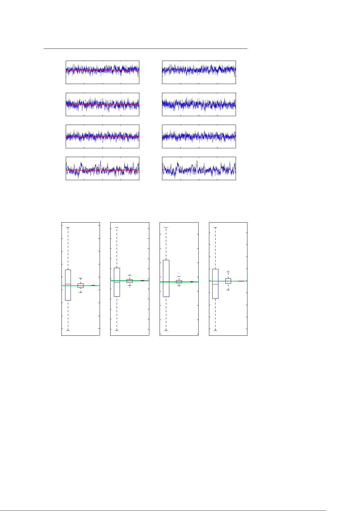
Noname man uscript No. (will b e inserted b y the editor) Zero V ariance Mark o v Chain Mon te Carlo for Ba yesian Estimators An tonietta Mira · Reza Solgi · Daniele Imparato Abstract Interest is in ev aluating, by Mark ov c hain Monte Carlo (MCMC) sim ulation, the expected v alue of a function with resp ect to a, p ossibly unnor- malized, probabilit y distribution. A general purp ose v ariance reduction tec h- nique for the MCMC estimator, based on the zero-v ariance principle intro- duced in the physics literature, is proposed. Conditions for asymptotic unbi- asedness of the zero-v ariance estimator are deriv ed. A central limit theorem is also pro ved under regularit y conditions. The p oten tial of the idea is illustrated with real applications to probit, logit and GARCH Ba yesian models. F or all these models, a cen tral limit theorem and un biasedness for the zero-v ariance estimator are pro ved (see the supplementary material a v ailable on-line). Keyw ords Control v ariates · GAR CH models · Logistic regression; · Metrop olis-Hastings algorithm · V ariance reduction 1 General idea The exp ected v alue of a function f with resp ect to a, p ossibly unnormalized, probabilit y distribution π , µ f = R f ( x ) π ( x ) d x / R π ( x ) d x is to b e ev aluated. Mark o v c hain Monte Carlo (MCMC) metho ds estimate in tegrals using a large but finite set of p oints, x i , i = 1 , · · · , N , collected along the sample path of an ergo dic Mark ov chain A. Mira Swiss Finance Institute, Univ ersity of Lugano, via Buffi 13, CH-6904 Lugano, Switzerland. E-mail: antonietta.mira@usi.c h R. Solgi Swiss Finance Institute, Universit y of Lugano, via Buffi 13, CH-6904 Lugano, Switzerland. E-mail: reza.solgi@usi.ch D. Imparato Department of Economics, Universit y of Insubria, via Mon te Generoso 71, 21100 V arese, Italy . E-mail: daniele.imparato@uninsubria.it 2 Antonietta Mira et al. ha ving π (normalized) as its unique stationary and limiting distribution ˆ µ f = P N i =1 f ( x i ) / N . In this pap er a general metho d is suggested to reduce the MCMC error by replacing f with a differen t function, ˜ f , obtained by prop erly re-normalizing f . The function ˜ f is constructed so that its exp ectation, under π , equals µ f , but its v ariance with resp ect to π is muc h smaller. T o this aim, a standard v ariance reduction tec hnique in tro duced for Mon te Carlo (MC) sim ulation, kno wn as control v ariates [39], is exploited. In the rest of this section we briefly explain the zero-v ariance (ZV) principle in tro duced in [4, 5]: an almost automatic metho d to construct control v ariates for MC sim ulation, in which an operator, H , acting as a map from functions to functions, and a trial function, ψ , are introduced. In quantum mec hanics, a commonly used op erator H is the so-called Hamil- tonian, whic h represents the total energy of the system, that is, the sum of the kynetic energy and the p otential energy , where the kinetic energy is typically defined as a second-order differen tial op erator. Suc h operator is Hermitian (that is, self-adjoint) if it acts on the restricted class of infinitely differentiable functions with compact support. If the trial function ψ b elongs to this class, and if H √ π = 0 (1) the re-normalized function defined as ˜ f ( x ) = f ( x ) + H ψ p π ( x ) (2) satisfies µ f = µ ˜ f : thus b oth f and ˜ f can be used to estimate the desired quan tity via Mon te Carlo or MCMC simulation. Ho wev er, for general ψ the condition µ f = µ ˜ f ma y not hold anymore and ad-hoc assumptions on the target π are necessary: this issue will b e further discussed in Section 5. Inspired by this physical setting, as a general framew ork H is supp osed to b e a Hermitian op erator (self-adjoint and real in all practical applications) satisfying (1), and the re-normalized function is defined as in (2): depending on the sp ecific choices of H and ψ , the condition µ f = µ ˜ f has to b e carefully v erified. Only a few op erators will b e considered in the pap er, the key one b eing the Hamiltonian differen tial op erator. An other important example discussed b elo w is the Marko v operator H acting as H ψ ( x ) = R K ( x , y ) ψ ( y ) d y , where K ( x , y ) needs to be symmetric. The re-normalized function, in this case, b e- comes ˜ f ( x ) = f ( x ) + R K ( x , y ) ψ ( y ) d y p π ( x ) . (3) and the condition µ f = µ ˜ f holds as a simple consequence of (1). Regardless of the sp ecific c hoice of the op erator and of the trial function, the optimal pair ( H , ψ ) , i.e. the one that leads to zero v ariance, can b e ob- tained by imp osing that ˜ f is constant and equal to its av erage, ˜ f = µ f , which Zero V ariance Marko v Chain Monte Carlo for Bay esian Estimators 3 is equiv alent to require that σ 2 ( ˜ f ) = 0, where σ 2 ( · ) denotes the v ariance op- erator with resp ect to the target π . The latter, together with (2), leads to the fundamen tal equation: H ψ = − p π ( x )[ f ( x ) − µ f ] . (4) In most practical applications equation (4) cannot be solved exactly , still, we prop ose to find an appro ximate solution in the follo wing wa y . First c ho ose a Hermitian operator H verifying (1). Second, parametrize ψ and derive the optimal parameters by minimizing σ 2 ( ˜ f ). The optimal parameters are then estimated using a first short MCMC simulation. Finally , a muc h longer MCMC sim ulation is p erformed using ˆ µ ˜ f instead of ˆ µ f as the estimator. This final estimator will b e called Zero V ariance (ZV) estimator through the pap er. Other research lines aim at reducing the asymptotic v ariance of MCMC estimators b y mo difying the transition k ernel of the Mark ov chain. These mod- ifications hav e b een achiev ed in many different wa ys, for example by trying to induce negativ e correlation along the chain path ([6, 21, 13, 41, 12]); b y trying to av oid random walk b ehavior via successive ov er-relaxation ([1, 36, 7]); by h ybrid Monte Carlo ([16, 35, 10, 18, 27]); by exploiting non reversible Marko v c hains ([15, 32]), by delaying rejection in Metrop olis-Hastings type algorithms ([45, 22]), by data augmentation ([46, 22]) and auxiliary v ariables ([43, 26, 33, 34]). Up to our knowledge, the only other research line that uses control v ari- ates in MCMC estimation follows the PhD thesis by [24] and has its most recen t developement in [14]. In [25] it is observed that, for any real-v alued function g defined on the state space of a Marko v chain { X n } , the one-step conditional exp ectation U ( x ) := g ( x ) − E [ g ( X n +1 ) | X n = x ] has zero mean with resp ect to the stationary distribution of the chain and can th us b e used as control v ariate. The Authors also note that the best c hoice for the function g is the solution of the associated P oisson equation whic h can rarely b e obtained analytically but can b e approximated in sp ecific settings. In [14], the use of this type of con trol v ariates is further explored in the setting of reversible Mark ov c hains were a closed form expression for U is often av ailable. In [4, 5] un biasedness and existence of a cen tral limit theorem (CL T) for the ZV estimator are not discussed, neither in [28], where this estimator is applied to a to y example. The main contributions of this pap er are, on the one hand, to deriv e the rigorous conditions for unbiasedness and CL T for the ZV estimators in MCMC simulation. On the other hand, we apply the ZV principle to some widely used mo dels (probit, logit, and GARCH) and demonstrate that, under v ery mild restrictions, the necessary conditions for unbiasedness and CL T are v erified. 2 Choice of H In this section guidelines to c ho ose the operator H , b oth for discrete and con tinuous settings, are giv en. In a discrete state space, denote with P ( x , y ) a transition matrix rev ersible with resp ect to π (a Mark ov chain will b e iden tified 4 Antonietta Mira et al. with the corresp onding transition matrix or kernel). W e restrict our attention in this section to op erators H acting as H f := P y K ( x , y ) f ( y ). The following c hoice K ( x , y ) = s π ( x ) π ( y ) [ P ( x , y ) − δ ( x − y )] (5) satisfies condition (1), where δ ( x − y ) is the Dirac delta function: δ ( x − y ) = 1 if x = y and zero otherwise. It should b e noted that the reversibilit y condition imp osed on the Mark o v chain is essen tial in order to hav e a symmetric op erator K ( x , y ), as required. With this c hoice of H , letting ˜ ψ = ψ / √ π , equation (3) b ecomes: ˜ f ( x ) = f ( x ) − X y P ( x , y )[ ˜ ψ ( x ) − ˜ ψ ( y )] . The same H can also be applied in contin uous settings. In this case, P is the k ernel of the Marko v chain and equation (5) can be trivially extended. This c hoice of H is exploited in [14], where the follo wing fundamen tal equation is found for the optimal ˜ ψ : E [ ˜ ψ ( x 1 ) | x 0 = x ] − ˜ ψ ( x ) = µ f − f ( x ). It is easy to pro ve that this equation coincides with our fundamental equation (4), with the c hoice of H given in (5). The Authors observe that the optimal trial function is giv en by ˜ ψ ( x ) = ∞ X n =0 [ E [ f ( x n ) | x 0 = x ] − µ f ] , (6) that is, ˜ ψ is the solution to the P oisson equation for f ( x ). Ho w ever, an explicit solution cannot b e obtained in general. Another op erator is prop osed in [4]: if x ∈ R d consider the Schr¨ odinger- t yp e Hamiltonian op erator: H f = − 1 2 d X i =1 ∂ 2 ∂ x 2 i f + V ( x ) f , (7) where V ( x ) is constructed to fulfill equation (1): V = 1 2 √ π ∆ √ π and ∆ denotes the Laplacian operator of second order deriv atives. In this setting, w e obtain the general expression for ˜ f rep orted in (2), where now H is the Schr¨ odinger- t yp e Hamiltonian. These are the op erator and the re-normalized function that will b e considered throughout this paper. Although it can only b e applied to con tinuous state spaces, this Sc hr¨ odinger-t yp e operator sho ws sev eral adv an- tages with resp ect to the op erator (5). First of all, in order to use (5) the conditional exp ectation app earing in (6) has to b e av ailable in closed form. Secondly , definition (7) do es not require rev ersibility of the Mark ov c hain. Moreo ver, this definition is indep endent of the kernel P ( x , y ) and, therefore, also of the type of MCMC algorithm that is used in the simulation. Note that, for calculating ˜ f b oth with the op erator (7) and (5), the normalizing constant of π is not needed. Zero V ariance Marko v Chain Monte Carlo for Bay esian Estimators 5 3 Choice of ψ The optimal choice of ψ is the exact solution of the fundamental equation (4). In real applications, typically , only approximate solutions, obtained b y min- imizing σ 2 ( ˜ f ), are av ailable. In other words, we select a functional form for ψ , parameterized by some co efficients of a class of p olynomials, and optimize those coefficients by minimizing the fluctuations of the resulting ˜ f . The par- ticular form of ψ is very dep endent on the problem at hand, that is on π , and on f . In the sequel it will b e assumed that ψ = P √ π , where P is a polynomial. As one would expect, the higher is the degree of the p olynomial, the higher is the num b er of control v ariates in tro duced and the higher is the v ariance reduction achiev ed. It can b e easily shown that in a d dimensional space, us- ing p olynomials of order p , provides  d + p d  − 1 control v ariates. How ever, some restrictions on the co efficients may o ccur in order to get an unbiased MCMC estimator. See Example 1 of Section 5 at this regard. 4 Control V ariates and optimal co efficients In this section, general expressions for the control v ariates in the ZV metho d are derived. Using the Schr¨ odinger-t yp e Hamiltonian H as given in (7) and trial function ψ ( x ) = P ( x ) p π ( x ), the re-normalized function is: ˜ f ( x ) = f ( x ) − 1 2 ∆P ( x ) + ∇ P ( x ) · z , (8) where z = − 1 2 ∇ ln π ( x ), ∇ =  ∂ ∂ x 1 , ..., ∂ ∂ x d  denotes the gradient and ∆ = P d i =1 ∂ 2 ∂ x 2 i . Lik e any other control v ariate (i.e. zero mean random v ariables under the distribution of in terest), the v ariable z can b e monitored to test con vergence along the lines suggested by [11] and [38], where the same control v ariate z = ∇ log π is used. Hereafter the function P is assumed to b e a p olynomial. As a first case, for P ( x ) = P d j =1 a j x j (1st degree p olynomial), one gets: ˜ f ( x ) = f ( x ) + H ψ ( x ) p π ( x ) = f ( x ) + a T z . The optimal c hoice of a , that minimizes the v ariance of ˜ f ( x ), is: a = − Σ − 1 zz σ ( z , f ) , where Σ zz = E ( z z T ) , σ ( z , f ) = E ( z f ) . F or a more general approach to the c hoice of coefficients using control v ariates, reference should b e made to [37] and [30]. W e an ticipate that conditions under whic h the ZV-MCMC estimator ob eys a CL T (Section 5) guaran tee that the optimal a is w ell defined. In ZV-MCMC, the optimal a is estimated in a first 6 Antonietta Mira et al. stage, through a short MCMC simulation 1 . When higher-degree p olynomials are considered, a similar formula for the co efficients asso ciated to the control v ariates is obtained once an explicit formula for the control v ariate v ector z has b een found. As an example, for quadratic p olynomials P ( x ) = a T x + 1 2 x T B x , the re-normalized ˜ f is : ˜ f ( x ) = f ( x ) − 1 2 tr( B ) + ( a + B x ) T z . Using second order p olynomials yields a vector of con trol v ariates of dimension 1 2 d ( d + 3). Therefore, finding the optimal coefficients requires w orking with Σ z z whic h is a matrix of dimension of order d 2 . This makes the use of second order p olynomials computationally exp ensive when dealing with high-dimensional sampling spaces, sa y of the order of decades. 5 Unbiasedness and cen tral limit theorem As remarked in Section 1, condition (1) ma y not b e sufficient to ensure unbi- asedness of the estimator when the Sc hr¨ odinger op erator (7) is used. In this section general conditionys on the target π are pro vided that guarantee that the ZV-MCMC estimator is (asymptotically) unbiased for the class of trial functions discussed. Details can b e found in the on-line supplemen tary mate- rial, App endix D. Prop osition 1 L et π b e a d -dimensional density on a b ounde d op en set Ω with r e gular b oundary ∂ Ω , whose first and se c ond derivatives ar e c ontinuous. Then, if ψ = P √ π , a sufficient c ondition for unbiase dness of the ZV-MCMC estimator is π ( x ) ∂ P ( x ) ∂ x j = 0 , for al l x ∈ ∂ Ω , j = 1 , . . . , d . The previous prop osition is a consequence of multidimensional integration by parts, from whic h one gets the equality E π  H ψ √ π  = 1 2 Z ∂ Ω [ ψ ∇ √ π − √ π ∇ ψ ] · n dσ, (9) where n denotes the versor orthogonal to ∂ Ω . When π has un b ounded supp ort, in tegration by parts cannot be used di- rectly . In this case, we can formulate the following result. Prop osition 2 L et π b e a d -dimensional density with unb ounde d supp ort Ω , whose first and se c ond derivatives ar e c ontinuous, and let ( B r ) r b e a se quenc e of b ounde d subsets, so that B r % Ω . Then, a sufficient c ondition for unbiase d- ness of the ZV-MCMC estimator is lim r → + ∞ Z ∂ B r π ∇ P · n dσ = 0 . 1 F rom a practical point of view there is no need to run t wo separate c hains, one to get the control v ariates and one to get the final ZV estimator: everything can b e done on a single Marko v chain which is run once to estimate the optimal coefficients of the control v ariates and then p ost-processed to get the ZV estimator. Zero V ariance Marko v Chain Monte Carlo for Bay esian Estimators 7 In the univ ariate case, if Ω is some interv al of the real line, that is, Ω = ( l , u ), where u, l ∈ R ∪ ±∞ , it is sufficient that dP ( x ) dx     x = l π ( l ) = dP ( x ) dx     x = u π ( u ) , (10) whic h is true, for example, if dP dx π annihilates at the b order of the supp ort. In the seminal pap er b y [4] unbiasedness conditions are not clearly explored since, t ypically , the target distribution the physicists are in terested in, anni- hilate at the b order of the domain with an exp onential rate. The following example shows how crucial the choice of trial functions is, in order to hav e an un biased estimator, even in trivial mo dels. Example 1 Let f ( x ) = x and π b e exp onen tial: π ( x ) = λe − λx I { x> 0 } . If P ( x ) is a first order p olynomial, (10) do es not hold and this choice do es not allow for a ZV-MCMC estimator, since the control v ariate z = − 1 2 d dx ln π ( x ) is constant and σ ( x, z ) = 0. How ever, to satisfy equation (10) it is sufficient to consider second order p olynomials. Indeed, if P ( x ) = a 0 + a 1 x + a 2 x 2 equation (10) is satisfied pro vided that a 1 = 0 and the minimization of the v ariance of ˜ f can b e carried out within this sp ecial class. The optimal c hoice a 2 := 1 2 λ yields zero v ariance: σ 2 ( ˜ f ) ≡ 0. 5.1 Cen tral limit theorem Conditions for existence of a CL T for ˆ µ f are w ell kno wn in the literature ([44]). Using these classical results, from (8) we hav e that the ZV-MCMC estimator ob eys a CL T provided f , ∆P and ∇ P · z b elong to L 2+ δ ( π ) when the Marko v c hain run for the simulation is geometrically ergodic. In the next corollary , the case of linear and quadratic polynomials P (used in the examples in Section 6) is considered. Corollary 1 L et ψ ( x ) = P ( x ) √ π , wher e P ( x ) is a first or se c ond de gr e e p olynomial. Then, the ZV-MCMC estimator ˆ µ ˜ f is a c onsistent estimator of µ f which satisfies the CL T, pr ovide d one of the fol lowing c onditions holds: C1 : The Markov chain is ge ometric al ly er go dic and f , x k i z j ∈ L 2+ δ ( π ) , ∀ i, j , for al l k ∈ { 0 , deg P − 1 } and some δ > 0 . C2 : The Markov chain is uniformly er go dic and f , x k i z j ∈ L 2 ( π ) , ∀ i, j and for al l k ∈ { 0 , deg P − 1 } . In the case of linear P , using the definition of control v ariate, the statemen t of the previous corollary can b e reformulated in this simple wa y: if f ∈ L 2 ( π ) and the chain is uniformly ergo dic, then a sufficient condition to get a CL T is m j = E π "  ∂ ∂ x j ln( π ( x ))  2 # < ∞ , ∀ j. 8 Antonietta Mira et al. The quan tity m j is kno wn in the literature as Linnik functional (if considered as a function of the target distribution, I ( π )) since it was introduced by [29]. The quan tity m j is also interpretable as the Fisher information of a lo cation family in a frequen tist setting. 5.2 Exp onen tial family Let π b elong to a d -dimensional exp onen tial family: π ( x ) ∝ exp( β · T ( x ) − K p ( β )) p ( x ), where β ∈ R d is the v ector of natural parameters. The follo wing theorem pro vides a sufficient condition for a CL T for ZV-MCMC estimators when the target b elongs to the exp onential family and a uniformly ergo dic Mark ov Chain is considered. Similar results can b e achiev ed when the Marko v Chain is geometrically ergo dic, by considering the 2 + δ momen t. This state- men t can b e easily verified by a direct computation. Theorem 1 L et π b elong to an exp onential family, with p such that ∂ log p ∂ x j ∈ L 2 ( π ) , ∀ i, k . Then, the Linnik functional of π is finite if and only if ∂ T k ∂ x j ∈ L 2 ( π ) , ∀ i, k . Example 2 The Gamma densit y Γ ( α, θ ) can be written as an exp onential fam- ily on (0 , + ∞ ), where p ( x ) ≡ 1, so that h yp otheses of Theorem 1 are satisfied. A direct computation shows that the Gamma density Γ ( α, θ ) has finite Linnik functional for any θ and for any α ∈ { 1 } ∪ (2 , + ∞ ). Under these conditions, a CL T holds for the ZV-MCMC estimator. 6 Examples In the sequel standard statistical models are considered. F or these mo dels, the ZV-MCMC estimators are derived in a Bay esian con text; from no w on, the target π = π ( β | x ) is the Bay esian p osterior distribution: therefore, the argumen t asso ciated with the state of the Marko v c hain is denoted by β instead of x , which represen ts, now, the vector of data. The op erator H considered is the Schr¨ odinger-type Hamiltonian defined in (7), and ψ = P √ π , where P is a p olynomial. Numerical simulations are provided, that confirm the effectiveness of v ari- ance reduction ac hieved, b y minimizing the v ariance of ˜ f within the class of trial functions considered. Moreo ver, conditions for b oth un biasedness and CL T for ˜ f are v erified for all the examples. F or the mathematical deriv ation of the zero-v ariance estimator and the proofs of un biasedness and CL T for the mo dels considered, w e refer the reader to the appendices of the on-line supplemen tary material (App endices A, B and C). Zero V ariance Marko v Chain Monte Carlo for Bay esian Estimators 9 6.1 Probit Mo del T o demonstrate the effectiveness of ZV for probit mo dels, a simple example is presented. The bank dataset from [17] contains the measurements of four v ariables on 200 Swiss banknotes (100 genuine and 100 counterfeit). The four measured v ariables x i ( i = 1 , 2 , 3 , 4), are the length of the bill, the width of the left and the right edge, and the b ottom margin width. These v ariables are used in a probit mo del as the regressors, and the type of the banknote y i , is the resp onse v ariable (0 for genuine and 1 for coun terfeit). Using flat priors, the Bay esian estimator of each parameter, β k , under squared error loss function, is the expected v alue of f k ( β ) = β k under π ( k = 1 , 2 , · · · , d ). The Ba yesian analysis of this problem is discussed in [31]. In order to find the op- timal v ector of parameters a k of the trial functions, a short Gibbs sampler, follo wing ([2]), (of length 2000, after 1000 burn in steps) is run, and the op- timal co efficients are estimated: ˆ a k = − ˆ Σ − 1 zz ˆ σ ( z , β k ). Finally another MCMC sim ulation of length 2000 is run (and using the estimated optimal v alues ob- tained in the previous step), along which e f k ( β ), for k = 1 , . . . , 4 is a veraged. W e ha ve rep eated this exp eriment 100 times. The MCMC traces of the ordi- nary MCMC and the ZV-MCMC in one of these MOnte Carlo exp erimen ts ha ve b een depicted in the left plot of Fig. 1. The blue curves are the traces of f k (ordinary MCMC), and the red ones are the traces of e f k (ZV-MCMC). It is clear from the figure that the v ariances of the estimator hav e substan tially decreased. Indeed for the linear trial functions, the ratios of the Monte Carlo estimates of the asymptotic v ariances of the tw o estimators (ordinary MCMC and ZV-MCMC) are b etw een 25 and 100. Even b etter p erformance can b e ac hieved using second degree polynomials to define the trial function. In the righ t column of Fig. 1 the traces of ZV-MCMC with second order P ( x ) are rep orted along with the traces of the ordinary MCMC. As it can b e seen from the figure, the v ariances of the ZV estimators are negligible: the ratio of the Mon te Carlo estimates of the asymptotic v ariances of the t w o estimators are b et ween 18 , 000 and 90 , 000. In this example (with the sim ulation length and burn-in rep orted ab ov e) the CPU time of ZV-MCMC is almost 3 times larger than the one of ordinary MCMC. In order to study the unbiasedness of the ZV-estimators empirically , w e ha ve run a very long MCMC (of length 10 8 ) and obtained a very narrow 95% confidence region for each parameter. In Fig. 2 we hav e depicted the b ox-plot of the ordinary MCMC (first b ox-plot), and the ZV-estimators (second and third b o x-plot) along with these 95% confidence regions (the green regions). As it can b e seen, the ZV-estimators are concen trated in the 95% confidence regions obtained from the v ery long chain. 10 Antonietta Mira et al. 0 500 1000 1500 2000 −3 −2 −1 0 1st Degree P(x) β 1 0 500 1000 1500 2000 −3 −2 −1 0 2nd Degree P(x) β 1 0 500 1000 1500 2000 −2 0 2 4 β 2 0 500 1000 1500 2000 −2 0 2 4 β 2 0 500 1000 1500 2000 −2 0 2 4 β 3 0 500 1000 1500 2000 −2 0 2 4 β 3 0 500 1000 1500 2000 0.5 1 1.5 2 β 4 0 500 1000 1500 2000 0.5 1 1.5 2 β 4 Fig. 1 Ordinary MCMC (blue) and ZV-MCMC (red) for probit mo del: ro ws are parameters, columns are degree p olynomials. −1.25 −1.24 −1.23 −1.22 −1.21 −1.2 −1.19 −1.18 −1.17 1 2 3 β 1 0.88 0.9 0.92 0.94 0.96 0.98 1 1.02 1.04 1.06 1.08 1 2 3 β 2 0.88 0.9 0.92 0.94 0.96 0.98 1 1.02 1 2 3 β 3 1.1 1.11 1.12 1.13 1.14 1.15 1.16 1.17 1.18 1 2 3 β 4 Fig. 2 Boxplots of ordinary MCMC estimates (1) and ZV-MCMC estimates (2 and 3) for the probit mo del, along with the 95% confidence region obtained by an ordinary MCMC of length 10 8 (green regions). Zero V ariance Marko v Chain Monte Carlo for Bay esian Estimators 11 −2.7 −2.65 −2.6 −2.55 −2.5 −2.45 1 2 3 β 1 1.7 1.8 1.9 2 2.1 2.2 1 2 3 β 2 1.95 2 2.05 2.1 2.15 2.2 2.25 2.3 2.35 1 2 3 β 3 2.1 2.12 2.14 2.16 2.18 2.2 2.22 2.24 2.26 2.28 1 2 3 β 4 Fig. 3 Box-plots of ordinary MCMC estimates (1) and ZV-MCMC estimates (2 and 3) for the logit mo del, along with the 95% confidence region obtained by an ordinary MCMC of length 10 8 (green regions). 6.2 Logit Mo del: A logit mo del is fitted to the same dataset of Swiss banknotes previously in- tro duced. Flat priors are used and, as b efore, the Bay esian estimator of each parameter, β k , (again under squared error loss functions) is the expected v alue of β k under π ( k = 1 , 2 , · · · , d ). Similar to the probit example, in the first stage a MCMC simulation is run, and the optimal parameters of P ( β ) are estimated. Then, in the second stage, an indep endent simulation is p erformed, and ˜ f k is a veraged, using the optimal trial function estimated in the first stage (the same sim ulation length and burn-in, as in the probit example, hav e b een used). F or linear p olynomial, the ratio of the Mon te Carlo estimates of the asymptotic v ariances of the tw o estimators (ordinary MCMC and ZV-MCMC) are b etw een 15 and 50. Using quadratic p olynomials, these ratios are b etw een 15 , 000 and 20 , 000. In this example the CPU time of the ZV-MCMC is almost 3 times higher than that of ordinary MCMC. W e hav e run a very long MCMC (of length 10 8 ) and obtained a v ery narro w 95% confidence region for each parameter. In Fig. 3 we hav e depicted the b ox-plot of the ordinary MCMC (first b ox-plot), and the ZV-estimators (second and third b ox-plot) along with these 95% confidence regions (the green regions). Again, as it can b e seen, the ZV-estimators are concen trated in the 95% confidence regions obtained from the v ery long Marko v chain. 12 Antonietta Mira et al. T able 1 GARCH v ariance reduction: 95% Confidence interv al for the ratio of the v ariances of ordinary MCMC estimators and ZV-MCMC estimator. ˆ ω 1 ˆ ω 2 ˆ ω 3 1st Degree P ( x ) 8-18 13-28 12-27 2nd Degree P ( x ) 1200-2700 6100-13500 6200-13800 3rd Degree P ( x ) 21000-47000 48000-107000 26000-58000 6.3 GAR CH Mo del Generalized autoregressiv e conditional heteroskedasticit y (GARCH) mo dels ([8]) ha ve b ecome one of the most imp ortant building blo c ks of mo dels in fi- nancial econometrics, where they are widely used to mo del returns. Here it is shown ho w the ZV-MCMC principle can b e exploited to estimate the pa- rameters of a univ ariate GAR CH mo del applied to daily returns of exchange rates in a Bay esian setting. Let S ( t ) b e the exchange rate at time t . The daily returns are defined as r ( t ) := [ S ( t ) − S ( t − 1)] /S ( t − 1) ≈ ln ( S ( t ) /S ( t − 1)). In a Normal-GAR CH model, w e assume the returns are conditionally Normally distributed, r ( t ) |F t ∼ N (0 , h t ), where h t = ω 1 + ω 3 h t − 1 + ω 2 r 2 t − 1 , and ω 1 > 0, ω 2 ≥ 0, and ω 3 ≥ 0 are the parameters of the model. The aim is to estimate the expected v alue of ω j under the p osterior π , using independent truncated normal priors. As an example, a Normal-GARCH(1, 1) is fitted to the daily returns of the Deutsche Mark vs British P ound exc hange rates from January 1985, to December 1987. In the first stage a short MCMC sim ulation ([3]) is used to estimate the optimal parameters of the trial function (2000 sweeps af- ter 1000 burn-in). In the second stage an indep endent s im ulation is run (with length 10000) and ˜ f k ( ω ) is a veraged in order to efficiently estimate the p oste- rior mean of each parameter. W e compare this ZV-MCMC with an ordinary MCMC of length 10000 (after 1000 burn-in). First, second and third degree p olynomials in the trial function are used. In order to study the eff ectiv eness of ZV-MCMC, w e hav e run these sim ulations (ordinary MCMC and ZV-MCMC) 100 times. As it can b e seen in T able 1, where a 95% confidence interv al for the v ariance reductions are rep orted, the ZV strategy reduces the v ariance of the estimators up to ten thousand times. In this example (with the sim ulation and burn-in lengths reported abov e) the CPU time of the ZV-MCMC is almost 20% higher than the CPU time of ordinary MCMC. In order to study the unbiasedness of the ZV-estimators empirically , w e ha ve run a v ery long MCMC (of length 10 7 ) and obtained a narro w 95% confidence region for eac h parameter. In Fig. 4 w e ha ve depicted the b ox- plot of the ordinary MCMC (first box-plot), and the ZV-estimators (second, third and fourth b ox-plots) along with these 95% confidence regions (the green regions). As it can b e seen the ZV-estimators lie in the range obtained by the v ery long MCMC. Zero V ariance Marko v Chain Monte Carlo for Bay esian Estimators 13 0.053 0.054 0.055 0.056 0.057 0.058 1 2 3 4 ω 0.236 0.238 0.24 0.242 0.244 0.246 0.248 0.25 0.252 1 2 3 4 α 0.58 0.585 0.59 0.595 0.6 0.605 0.61 1 2 3 4 β Fig. 4 Boxplots of ordinary MCMC estimates (1) and ZV-MCMC estimates (2, 3 and 4) for the GARCH model, along with the 95% confidence region obtained by an ordinary MCMC of length 10 7 (green regions). Finally , note that the ZV strategy can b e used in great generality and can b e applied also to more complex GARCH mo dels (such as E-GARCH, I-GAR CH, Q-GAR CH, GJR-GAR CH, [9]), provided it is p ossible to analiti- cally compute the necessary deriv ativ es and v erify the hypotheses needed for un biasedness and CL T, in a wa y similar to the pro of rep orted in App endix C. 7 Discussion Cross-fertilizations b etw een physics and statistical literature hav e prov ed to b e quite effective in the past, esp ecially in the MCMC framework. The first paradigmatic example is the pap er b y [23] first and [19] later on. Besides translating in to statistical terms the pap er b y [4], the main effort of our work has b een the discussion of unbiasedness and conv ergence of the ZV-MCMC estimator. The study of CL T leads to the condition of finiteness for E π [( ∂ log π ( x ) ∂ x ) 2 ]. This quan tity has also b een used in the recen t paper b y [20] as a metric tensor to improv e efficiency in Langevin diffusion and Hamiltonian MC metho ds. Their idea is to choose this metric as an optimal, lo cal tuning of the dynamic, which is able to take into account the intrinsic anisotropy in the mo del considered. In our understanding, what makes these metho ds and our extremely efficient, is the common strategy of exploiting information con tained 14 Antonietta Mira et al. in the deriv atives of the log-target. A com bination of the tw o strategies could b e explored: once the deriv ativ es of the log-target are computed, they can b e used both to b o ost the p erformance of the Mark ov chain (as suggested b y [20]) and to achiev e v ariance reduction by using them to design control v ariates. This is particularly easy since control v ariates can b e constructed by simply p ost-pro cessing the Mark ov chain and, thus, there is no need to re-run the sim ulation. The second main contribution of this pap er is the critical discussion of the selection of H and ψ . A comparison b etw een the v ariance reduction framework exploited in [14] and the choice of different op erators H in our context has remark ed contras and b enefits of the tw o approaches. Differen t choices of H and ψ could provide alternative efficien t v ariance reduction strategies. This can b e easily achiev ed b y considering a wider class of trial functions: ψ ( x ) = P ( x ) q ( x ), where, as b efore, P ( x ) denotes a parametric class of polynomials, and q ( x ) is an arbitrary (sufficiently regular) function. In the presen t research w e hav e explored ψ based on first, second and third degree p olynomials. Despite the use of this fairly restrictive class of trial functions, the degree of v ariance reduction obtained in the examples in Section 6 and in other simulation studies (not rep orted here) is impressive and of the order of ten times (for first degree p olynomials) and of thousand times (for higher degree p olynomials), with practically small extra CPU time needed in the sim ulation. Finally , mention should b e made to an alternativ e, more general renormal- ized function ˜ f rep orted in the pap er by [5], defined as: ˜ f = f + H ψ √ π − ψ ( H √ π ) π , (11) where, again, H is an Hamiltonian op erator and ψ a quite arbitrary trial function. In this setting, if H = − 1 2 ∆ + V , under the same, mild conditions discussed in Section 5, ˜ f has the same exp ectation as f under π . This is true without imp osing condition (1), so that now V can b e also chosen arbitrarily . Therefore, the re-normalization (11) allows for a more general class of Hamil- tonians. Supplemen tary Materials Supplemen tary materials are av ailable. In App endices A, B and C the zero v ariance estimator and the pro of of CL T are given for all the examples. In App endix D computations of unbiasedness conditions discussed in Section 5 are rep orted and v erified for the three examples. Ac kno wledgemen t Thanks are due to D. Bressanini, for bringing to our attention the pap er b y Assaraf and Caffarel and helping us translate it in to statistical terms; to Zero V ariance Marko v Chain Monte Carlo for Bay esian Estimators 15 prof. E. Regazzini and F. Nicola, for discussing the CL T conditions for the examples; P . T enconi, F. Carone and F. Leisen for commen ts and contributions to a preliminary version of this research. And finally , Assaraf and Caffarel themselv es hav e given us interesting and useful comments that hav e greatly impro ved the pap er. App endix A: Probit mo del Mathematical form ulation Let y i b e Bernoulli r.v.’s: y i | x i ∼ B (1 , p i ) , p i = Φ ( x T i β ), where β ∈ R d is the vector of parameters of the mo del and Φ is the c.d.f. of a standard normal distribution. The lik eliho o d function is: l ( β | y , x ) ∝ n Y i =1  Φ ( x T i β )  y i  1 − Φ ( x T i β )  1 − y i . As it can b e seen by insp ection, the likelihoo d function is in v ariant under the transformation ( x i , y i ) → ( − x i , 1 − y i ). Therefore, for the sak e of simplicity , in the rest of the example w e assume y i = 1 for an y i , so that the likelihoo d simplifies: l ( β | y , x ) ∝ n Y i =1 Φ ( x T i β ) . This formula shows that the contribution of x i = 0 is just a constant Φ ( x T i β ) = Φ (0) = 1 2 , therefore, without loss of generalit y , we assume for all i , x i 6 = 0 . Using flat priors, the p osterior of the mo del is prop ortional to the likeli- ho o d, and the Ba yesian estimator of each parameter, β k , is the exp ected v alue of f k ( β ) = β k under π ( k = 1 , 2 , · · · , d ). Using Sc hr¨ odinger-t yp e Hamiltonians, H and ψ k ( β ) = P k ( β ) p π ( β ), as the trial functions, where P k ( β ) = P d j =1 a j,k β j is a first degree p olynomial, one gets: e f k ( β ) = f k ( β ) + H ψ k ( β ) p π ( β | y , x ) = f k ( β ) + d X j =1 a j,k z j , where, for j = 1 , 2 , . . . , d , z j = − 1 2 n X i =1 x ij φ ( x T i β ) Φ ( x T i β ) , b ecause of the assumption y i = 1 for an y i . 16 Antonietta Mira et al. Cen tral limit theorem In the followin g, it is supp osed that P is a linear p olynomial. In the Probit mo del, the ZV-MCMC estimators ob ey a CL T if z j ha ve finite 2 + δ moment under π , for some δ > 0: E π  | z j | 2+ δ  = c 1 E π        n X i =1 x ij φ ( x T i β ) Φ ( x T i β )      2+ δ   = c 1 c 2 Z R d      n X i =1 x ij φ ( x T i β ) Φ ( x T i β )      2+ δ n Y i =1 Φ ( x T i β ) dβ < ∞ . where c 1 = 2 − 2 − δ , and c 2 is the normalizing constant of π (the target poste- rior). Define: K 1 ( β ) =      n X i =1 x ij φ ( x T i β ) Φ ( x T i β )      2+ δ , K 2 ( β ) = n Y i =1 Φ ( x T i β ) , K ( β ) = K 1 ( β ) K 2 ( β ) and therefore: E π  | z j | 2+ δ  = c Z R d K 1 ( β ) K 2 ( β ) dβ . where c = c 1 c 2 . Before studying the conv ergence of this integral, the following prop ert y of the likelihoo d for the probit mo del is needed. Prop osition 3 Existenc e and uniqueness of MLE implies that, for any β 0 ∈ R d \ { 0 } , ther e exists i such that x T i β 0 < 0 . Pro of (b y contradiction). Uniqueness of MLE implies that x T x is full rank, that is, there is no β 0 orthogonal to all observ ations x i . This can be seen b y con tradiction: singularity of x T x implies existence of a non-zero β 0 orthogonal to all observ ations x i . This fact, in turn, implies l ( β | x , y ) = l ( β + cβ 0 | x , y ) and, therefore, l ( •| x , y ) do es not hav e a unique global maximum. Next, assume there exists some β 0 ∈ R d suc h that, for an y i , x T i β 0 > 0. Then β 0 is a direction of recession for the negative log-lik eliho o d function − P n i =1 ln Φ ( x T i β ) (that is a prop er closed conv ex function). This implies that this function do es not hav e non-empty b ounded minimum set ([40]), which means that the MLE do es not exist.  No w, rewriting R R d K ( β ) dβ in h yp er-spherical coordinates through the bijec- tiv e transformation ( ρ, θ 1 , . . . , θ d − 1 ) := F ( β ), where F − 1 is defined as Zero V ariance Marko v Chain Monte Carlo for Bay esian Estimators 17            β 1 = ρ cos( θ 1 ) β l = ρ cos( θ l ) Q l − 1 m =1 sin( θ m ) , for l = 2 , ..., d − 1 β d = ρ Q d − 1 m =1 sin( θ m ) , (12) for θ ∈ Θ := { 0 ≤ θ i ≤ π , i = 1 , . . . , d − 2, 0 ≤ θ d − 1 < 2 π } and ρ > 0, one gets Z R d K ( β ) dβ = Z Θ Z + ∞ 0 K ( F − 1 ( ρ, θ )) ρ d − 1 d − 2 Y j =2 sin d − j ( θ j − 1 ) dρdθ . ≤ Z Θ Z + ∞ 0 K ( F − 1 ( ρ, θ )) ρ d − 1 dρdθ := Z Θ A ( θ ) dθ , Observ e that the integrand is well defined for any ( ρ, θ ) on the domain of in tegration, so it is enough to study its asymptotic b ehaviour when ρ goes to infinit y , and θ ∈ Θ . First, analyze K 1 ( F − 1 ( ρ, θ )) =      n X i =1 x ij φ ( | x i | ρλ i ( θ ) Φ ( | x i | ρλ i ( θ ))      2+ δ , where, for an y i , λ i is a suitable function of the angles θ such that λ i ∈ [ − 1 , 1], which tak es into account the sign of the scalar pro duct in the original co ordinates system. F or any i , when ρ → ∞ – if λ i < 0, x ij φ ( | x i | ρλ i ) Φ ( | x i | ρλ i ) ∈ O ( ρ ); – if λ i > 0, x ij φ ( | x i | ρλ i ) Φ ( | x i | ρ ) λ i ∈ O ( φ ( λ i ρ )); – if λ i = 0, x ij φ ( | x i | ρλ i ) Φ ( | x i | ρλ i ) = x ij q 2 π ∈ O (1). Therefore: n X i =1 x ij φ ( | x i | ρλ i ) Φ ( | x i | ρλ i ) ∈ O ( ρ ) and, for an y θ ∈ Θ : K 1 ( F − 1 ( ρ, θ )) ∈ O  ρ 2+ δ  . Now, fo cus on K 2 ( F − 1 ( ρ, θ )) = Q n i =1 Φ ( | x i | ρλ i ( θ )); existence of MLE for the probit mo del implies that, for an y θ ∈ Θ , there exists some l (1 ≤ l ≤ n ), such that λ l ( θ ) < 0, and therefore: K 2 ( F − 1 ( ρ, θ )) < Φ ( | x l | ρλ l ) ∈ O ( φ ( λ l ρ )) ρ → ∞ . (13) Putting these results together leads to K ( F − 1 ( ρ, θ )) = K 1 ( F − 1 ( ρ, θ )) K 2 ( F − 1 ( ρ, θ )) ∈ O  ρ 2+ δ φ ( λ l ( θ ) ρ )  18 Antonietta Mira et al. so that, for an y θ ∈ Θ , K ( F − 1 ( ρ, θ )) ρ d − 1 ∈ O  ρ 1+ δ + d φ ( λ l ( θ ) ρ )  , ρ → + ∞ . Therefore, whenev er the v alue θ ∈ Θ , its in tegrand con verges to zero rapidly enough when ρ → + ∞ . This concludes the pro of. Note 1 . In ([42]) it is shown that the existence of the p osterior under flat priors for probit and logit models is equiv alent to the existence and finite- ness of MLE. This ensures us that the p osterior is well defined in our con- text. In order to verify the existence of the p osterior mean, w e can use a simplified version of the pro of giv en ab ov e. In other words we should show R β j Q n i =1 Φ ( x T i β ) dβ < + ∞ , that is, K 1 ( β ) = β j ∈ O ( ρ ). Therefore, a weak er v ersion of the pro of given ab ov e can b e employ ed. Note 2 . In the proof giv en abov e we hav e used flat priors: although this assumption simplifies the pro of, how ever a v ery similar proof can be applied for non-flat priors. Assume the prior is π 0 ( β ). Under this assumption the posterior is π ( β ) = π 0 ( β ) l ( β | y , x ) ∝ π 0 ( β ) Q n i =1 Φ ( x T i β ) and the con trol v ariates are: z j = − 1 2 d ln π 0 ( β ) dβ j − 1 2 P n i =1 x ij φ ( x T i β ) Φ ( x T i β ) . Therefore we need to prov e the 2 + δ -th momen t of z j under π ( β ) is finite. A sufficien t condition for this is the finiteness of 2 + δ -th momen ts of − 1 2 d ln π 0 ( β ) dβ j and − 1 2 P n i =1 x ij φ ( x T i β ) Φ ( x T i β ) under π ( β ). If we assume π 0 ( β ) is b ounded ab ov e, the latter is a trivial consequence of the pro of giv en ab ov e for the flat priors. Therefore we only need to prov e the finiteness of the in tegral Z R d     d ln π 0 ( β ) dβ j     2+ δ π 0 ( β ) n Y i =1 Φ ( x T i β ) dβ . Again if w e assume the prior is b ounded from ab ov e, a sufficient condition for the existence of this in tegral is the existence of the following integral: Z R d     d ln π 0 ( β ) dβ j     2+ δ n Y i =1 Φ ( x T i β ) dβ A proof very similar to the one giv en abov e will show that this in tegral is finite for common c hoices of priors π 0 ( β ) (such as Normal, Student’s T, etc). App endix B: Logit mo del Mathematical form ulation In the same setting as the probit mo del, let p i = exp( x T i β ) 1+exp( x T i β ) where β ∈ R d is the v ector of parameters of the mo del. The likelihoo d function is: l ( β | y , x ) ∝ n Y i =1  exp( x T i β ) 1 + exp( x T i β )  y i  1 1 + exp( x T i β )  1 − y i . (14) Zero V ariance Marko v Chain Monte Carlo for Bay esian Estimators 19 By inspection, it is easy to v erify that the lik eliho o d function is in v arian t under the transformation:( x i , y i ) → ( − x i , 1 − y i ). Therefore, for the sake of simplicit y , in the sequel w e assume y i = 0 for any i , so that the likelihoo d simplifies as: l ( β | y , x ) ∝ n Y i =1 1 1 + exp( x T i β ) . The con tribution of x i = 0 to the likelihoo d is just a constan t, therefore, without loss of generality , it is assumed that x i 6 = 0 for all i . Using flat priors, the posterior distribution is prop ortional to (14) and the Ba y esian estimator of each parameter, β k , is the exp ected v alue of f k ( β ) = β k under π ( k = 1 , 2 , · · · , d ). Using the same pair of op erator H and test function ψ k as in App endinx A, the con trol v ariates are: z j = 1 2 n X i =1 x ij exp( x T i β ) 1 + exp( x T i β ) , for j = 1 , 2 , . . . , d. Cen tral limit theorem As for the probit mo del, the ZV-MCMC estimators ob ey a CL T if the control v ariates z j ha ve finite 2 + δ momen t under π , for some δ > 0 : E π  z 2+ δ j  = c 1 E π   n X i =1 x ij exp( x T i β ) 1 + exp( x T i β ) ! 2+ δ   = c 1 c 2 Z R d n X i =1 x ij exp( x T i β ) 1 + exp( x T i β ) ! 2+ δ n Y i =1 1 1 + exp( x T i β ) dβ where c 1 = 2 − 2 − δ , and c 2 is the normalizing constan t of π . The finitiness of the in tegral is, indeed, trivial. Observ e that the function e y / (1 + e y ) is bounded b y 1; therefore, E π  z 2+ δ j  ≤ n X i =1 x ij ! 2+ δ < ∞ . As for probit mo del, note that it can easily b e shown that the p osterior means exist under flat priors. Moreov er, a very similar pro of (see Note 2 of App endix A) can b e used under a normal or Studen t’s T prior distribution. App endix C: GAR CH mo del Mathematical form ulation W e assume that the returns are conditionally normal distributed, r ( t ) |F t ∼ N (0 , h t ), where h t is a predictable ( F t − 1 measurable process): h t = ω 1 + 20 Antonietta Mira et al. ω 3 h t − 1 + ω 2 r 2 t − 1 , where ω 1 > 0, ω 2 ≥ 0, and ω 3 ≥ 0. Let r = ( r 1 , . . . , r T ) be the observ ed time series. The likelihoo d function is equal to: l ( ω 1 , ω 2 , ω 3 | r ) ∝ T Y t =1 h t ! − 1 2 exp − 1 2 T X t =1 r 2 t h t ! and using indep endent truncated Normal priors for the parameters, the p os- terior is: π ( ω 1 , ω 2 , ω 3 | r ) ∝ exp  − 1 2  ω 2 1 σ 2 ( ω 1 ) + ω 2 2 σ 2 ( ω 2 ) + ω 2 3 σ 2 ( ω 3 )  T Y t =1 h t ! − 1 2 exp − 1 2 T X t =1 r 2 t h t ! . Therefore, the con trol v ariates (when the trial function is a first degree p oly- nomial) are: ∂ ln π ∂ ω i = − ω i σ 2 ( ω i ) − 1 2 T X t =1 1 h t ∂ h t ∂ ω i + 1 2 T X t =1 r 2 t h 2 t ∂ h t ∂ ω i , i = 1 , 2 , 3 , where: ∂ h t ∂ ω 1 = 1 − ω t − 1 3 1 − ω 3 , ∂ h t ∂ ω 2 =  r 2 t − 1 + ω 3 ∂ h t − 1 ∂ ω 2  I t> 1 , ∂ h t ∂ ω 3 =  h t − 1 + ω 3 ∂ h t − 1 ∂ ω 3  I t> 1 . Cen tral limit theorem In order to prov e the CL T for the ZV-MCMC estimator in the Garch mo del, w e need: ∂ ln π ∂ ω 2 , ∂ ln π ∂ ω 3 , ∂ ln π ∂ ω 1 ∈ L 2+ δ ( π ) . (15) T o this end, h t and its partial deriv atives should b e expressed as a function of h 0 and r : h t = ω 1 ( t − 1 X k =1 1 + ω k 3 ) + ω t 3 h 0 + ω 2 ( t − 1 X k =1 1 + ω k 3 r 2 t − 1 − k ) , ∂ ln h t ∂ ω 1 = 1 − ω t − 1 3 1 − ω 3 I { t> 1 } , ∂ ln h t ∂ ω 2 =   r 2 t − 1 + t − 2 X j =0 ω t − 1 − j 3 r 2 j   I { t> 1 } , ∂ ln h t ∂ ω 3 =   h t − 1 + t − 2 X j =0 ω t − 1 − j 3 h j   I { t> 1 } . Zero V ariance Marko v Chain Monte Carlo for Bay esian Estimators 21 Next, mo ving to spherical co ordinates, the integral (15) can b e written as Z [0 ,π / 2] 2 Z ∞ 0 K j ( ρ ; θ , φ ) dρdθ dφ := Z [0 ,π / 2] 2 A j ( θ , φ ) dθ dφ, where, for j = 1 , 2 , 3, K j ( · ; θ , φ ) = | W j | 2+ δ × W , with W 1 = − 1 σ 2 ( ω 1 ) ρ cos θ sin φ − 1 2 T X t =2  1 ˜ h t − r 2 t ˜ h 2 t  1 − ρ t − 1 cos t − 1 φ 1 − ρ cos φ , W 2 = − 1 σ 2 ( ω 2 ) ρ sin θ sin φ − 1 2 T X t =2  1 ˜ h t − r 2 t ˜ h 2 t    r 2 t − 1 + t − 2 X j =0 x t − 1 − j 3 r 2 j   , W 3 = − 1 σ 2 ( ω 3 ) ρ cos φ − 1 2 T X t =2  1 ˜ h t − r 2 t ˜ h 2 t    ˜ h t − 1 + t − 2 X j =0 x t − 1 − j 3 ˜ h j   , W = exp − 1 2 ρ 2 ( 1 σ 2 ( ω 1 ) cos 2 θ sin 2 φ + 1 σ 2 ( ω 2 ) sin 2 θ sin 2 φ + 1 σ 2 ( ω 3 ) cos 2 φ ) − 1 2 T X t =1 r 2 t ˜ h 2 t ! × × ρ 2 sin θ T Y t =1 ˜ h t ! − 1 2 (16) and ˜ h t = − ρ cos θ sin φ t − 1 X k =1 (1+ ρ k cos k φ )+ h 0 ρ t cos t φ + ρ sin θ sin φ t − 1 X k =1 (1+ r 2 t − 1 − k ρ k cos k φ ) . The aim is to prov e that, for an y θ, φ ∈ [0 , π / 2] and for an y j , A j ( θ , φ ) is finite. T o this end, the conv ergence of A j for an y θ , φ should b e discussed. Let us study the prop er domain of K j ( · ; θ , φ ). Observe that K j ( · ; θ , φ ) is not defined whenever ˜ h t = 0 and, if j = 1 and φ 6 = π / 2, also for ρ = 1 / cos φ . Ho wev er, the discontin uity of K 3 at this p oin t is remo v able, so that the domain of K 3 can b e extended b y contin uity also at ρ = 1 / cos φ . Since ˜ h t = 0 if and only if ρ = 0, it can be concluded that, for an y j and for an y θ , φ ∈ [0 , π / 2], the prop er domain of K j ( · ; θ , φ ) is dom K j ( · ; θ , φ ) = (0 + ∞ ) . By fixing the v alue of θ and φ , let us study the limits of K j when ρ → 0 and ρ → + ∞ . Observe that, whatev er the v alues of θ and φ are, W j ’s are rationale functions of ρ . Therefore, for any j , | W j | 2+ δ cannot gro w to wards infinity more than p olynomially at the b oundary of the domain. On the other hand, W go es to zero with an exp onen tial rate b oth when ρ → 0 and ρ → + ∞ , for an y θ and φ . This is sufficien t to conclude that, for any θ , φ ∈ [0 , π / 2], the integral A j is finite for j = 1 , 2 , 3 and, therefore, condition (15) holds and the ZV estimators for the GAR CH mo del ob eys a CL T. 22 Antonietta Mira et al. App endix D: un biasedness In this App endix, explicit computations are presen ted, which were omitted in Section 5. Moreov er, it is prov ed that all the ZV-MCMC estimators discussed in Section 8 are un biased. F ollowing the same notations as in Section 5, equation (9) follows b ecause  H ψ √ π  := Z Ω H ψ √ π = Z Ω ( V ψ √ π − 1 2 ∆ψ √ π ) = Z Ω V √ π ψ − 1 2 Z ∂ Ω √ π ∇ ψ · n dσ + 1 2 Z Ω ∇ √ π · ∇ ψ = Z Ω V √ π ψ − 1 2 Z ∂ Ω √ π ∇ ψ · n dσ + 1 2 Z ∂ Ω ψ ∇ √ π · n dσ − 1 2 Z Ω ψ ∆ √ π = Z Ω ( H √ π ) ψ + 1 2 Z ∂ Ω [ ψ ∇ √ π − √ π ∇ ψ ] · n dσ = 1 2 Z ∂ Ω [ ψ ∇ √ π − √ π ∇ ψ ] · n dσ. Therefore,  H ψ √ π  = 0 if ψ ∇ √ π = √ π ∇ ψ on ∂ Ω . Now, let ψ = P √ π . Then, ∇ ψ = √ π ∇ P + P 2 √ π ∇ π , so that  H ψ √ π  = 0 if π ( x ) ∂ P ( x ) ∂ x j = 0 , ∀ x ∈ ∂ Ω , j = 1 , . . . , d. When π has un b ounded supp ort, following the previous computations inte- grating o ver the b ounded set B r and taking the limit for r → ∞ , one gets  H ψ √ π  = 1 2 lim r → + ∞ Z ∂ B r π ∇ P · n dσ. (17) Therefore, unbiasedness in the unbounded case is reached if the limit appearing in the righ t-hand side of (17) is zero. No w, the un biasedness of the ZV-MCMC estimators exploited in Section 8 is discussed. T o this end, condition (17) should b e v erified. Let B ρ b e a h yp er-sphere of radius ρ and let n := 1 ρ β b e its normal v ersor. Then, for linear P , (17) equals zero if, for an y j = 1 , . . . , d , lim ρ → + ∞ 1 ρ Z B ρ π ( β ) β j dS = 0 . (18) Zero V ariance Marko v Chain Monte Carlo for Bay esian Estimators 23 The Probit mo del is first considered. By using the same notations as in App endix A, the in tegral in (18) is prop ortional to lim ρ → + ∞ 1 ρ Z Θ K 2 ( F − 1 ( ρ, θ )) ρ d dθ . (19) Note that, b ecause of (13), there exist ρ 0 and M suc h that K 2 ( F − 1 ( ρ, θ )) ρ d ≤ M φ ( λ l ( θ ) ρ ) ρ d ≤ M φ ( λ l ( θ ) ρ 0 ) ρ d 0 := G ( θ ) ∀ ρ ≥ ρ 0 . Since G ( θ ) ∈ L 1 , by the dominated conv ergence theorem a sufficient condition to get un biasedness is lim ρ → + ∞ K 2 ( F − 1 ( ρ, θ )) ρ d − 1 = 0 , (20) whic h is true, b ecause of (13) for the Probit mo del. W e no w consider the Logit mo del for which it is easy to prov e that Prop o- sition 3 holds. As done for the Probit mo del, one can write E π  z 2+ δ j  ∝ Z R d K 1 ( β ) K 2 ( β ) dβ , where K 1 ( β ) = n X i =1 x ij exp( x T i β ) 1 + exp( x T i β ) ! 2+ δ , K 2 ( β ) = n Y i =1 1 1 + exp( x T i β ) , By using the h yp er-spherical change of v ariables in (12), we get E π  z 2+ δ j  ∝ Z Θ Z ∞ 0 K 1 ( F − 1 ( ρ, θ )) K 2 ( F − 1 ( ρ, θ )) ρ d − 1 dρ : and, as for the Probit mo del, w e m ust v erify Equation (19). No w analyze K 2 ( F − 1 ( ρ, θ )); for any θ , existence of MLE implies the existence of some l (1 ≤ l ≤ n ), such that λ l ( θ ) > 0, and therefore: K 2 ( F − 1 ( ρ, θ )) = n Y i =1 1 1 + exp( | x i | ρλ i ) < 1 1 + exp( | x l | ρλ l ) ∈ O (exp( − ρλ l )) . (21) 24 Antonietta Mira et al. Therefore, there exist ρ 0 , M suc h that K 2 ( F − 1 ( ρ, θ )) ρ d ≤ M exp( − λ l ( θ ) ρ ) ρ d ≤ M exp( − λ l ( θ ) ρ 0 ) ρ d 0 := G ( θ ) ∀ ρ ≥ ρ 0 , where G ( θ ) ∈ L 1 . These computations allow us to use Equation (20) as a sufficien t condition to get unbiasedness, and its pro of b ecomes trivial. Finally consider the GARCH mo del. In this case, B ρ is the p ortion of a sphere of radius ρ defined on the p ositiv e orthant. Then, the limit lim ρ → + ∞ 1 ρ Z [0 ,π / 2] 2 W ( F − 1 ( ρ, θ )) ρ d dθ , where W was defined in (16), should b e discussed. Again, an application of the dominated con vergence theorem leads to the simpler condition lim ρ → + ∞ W ( F − 1 ( ρ, θ )) ρ 2 = 0 , whic h is true, since W decays with an exp onential rate. References 1. Adler, S.: Over-relaxation metho d for the Monte Carlo ev aluation of the partition func- tion for multiquadratic actions. Phys. Rev. D 23 , 2901–2904 (1981) 2. Alb ert, J., Chib, S.: Bay esian analysis of binary and p olychotomous resp onse data. Journal of the American Statistical Asso ciation 88, 422 , 669–679 (1993) 3. Ardia, D.: Financial risk management with bay esian estimation of GARCH mo dels: Theory and applications. In: Lecture Notes in Economics and Mathematical Systems 612. Springer-V erlag (2008) 4. Assaraf, R., Caffarel, M.: Zero-Variance principle for Monte Carlo algorithms. Physical Review letters 83, 23 , 4682–4685 (1999) 5. Assaraf, R., Caffarel, M.: Zero-v ariance zero-bias principle for observ ables in quantum Monte Carlo: Application to forces. The Journal of Chemical Physics 119, 20 , 10,536– 10,552 (2003) 6. Barone, P ., F rigessi, A.: Impro ving sto chastic relaxation for Gaussian random fields. Probability in the Engineering and Informational Sciences 4 , 369–389 (1989) 7. Barone, P ., Sebastiani, G., Stander, J.: General o ver-relaxation Marko v chain Monte Carlo algorithms for Gaussian densities. Statistics & Probability Letters 52,2 , 115–124 (2001) 8. Bollerslev, T.: Generalized autoregressive conditional heteroskedasticit y . Journal of Econometrics 31, 3 , 307–327 (1986) 9. Bollerslev, T.: Glossary to ARCH (GARCH). In: V olatility and Time Series Economet- rics, Essays in Honor of Rob ert Engle, Edited by Tim Bollerslev, Jeffrey Russell and Mark W atson. Oxford University Press, Oxford, UK (2010) 10. Brewer, M., Aitken, C., T albot, M.: A comparison of hybrid strategies for Gibbs sam- pling in mixed graphical mo dels. Computational Statistics 21 , 343–365 (1996) 11. Bro oks, S., Gelman, A.: Some issues in monitoring conv ergence of iterativ e simulations. Computing Science and Statistics (1998) 12. Craiu, R., Lemeieux, C.: Acceleration of the m ultiple-try Metropolis algorithm using antithetic and stratified sampling. Journal Statistics and Computing 17, 2 , 109–120 (2007) Zero V ariance Marko v Chain Monte Carlo for Bay esian Estimators 25 13. Craiu, R., Meng, X.: Multiprocess parallel an tithetic coupling for backw ard and forw ard Marko v chain Monte Carlo. The A nnals of Statistics 33, 2 , 661–697 (2005) 14. Dellap ortas, P ., Konto yiannis, I.: Con trol v ariates for estimation based on rev ersible Marko v c hain Monte Carlo samplers. Journal of the Roy al Statistical So ciety , Series B. 74(1) , 133–161 (2012) 15. Diaconis, P ., Holmes, S., Neal, R.F.: Analysis of a nonreversible Marko v chain sampler. Ann. Appl. Probab. 10,3 , 726–752 (2000) 16. Duane, S., Kennedy , A., Pendleton, B., Row eth, D.: Hybrid Monte Carlo. Ph ysics Letters B 195 , 216–222 (2010) 17. Flury , B., Riedwyl, H.: Multiv ariate Statistics. Chapman and Hall (1988) 18. F ort, G., Moulines, E., Rob erts, G., Rosenthal, S.: On the geometric ergodicity of h ybrid samplers. Journal of Applied Probability 40, 1 , 123–146 (2003) 19. Gelfand, A., Smith, A.: Sampling-based approaches to calculating marginal densities. J. American Statistical Asso ciation 85 , 398–409 (1990) 20. Girolami, M., Calderhead, B.: Riemannian manifold Langevin and Hamiltonian Monte Carlo metho ds. J. R. Statist. Soc. B 73, 2 , 1–37 (2011) 21. Green, P ., Han, X.: Metrop olis metho ds, Gaussian prop osals, and antithetic v ariables. In: P . Barone, A. F rigessi, M. Piccioni (eds.) Lecture Notes in Statistics, Sto chastic Methods and Algorithms in Image Analysis, v ol. 74, pp. 142–164. Springer V erlag (1992) 22. Green, P .J., Mira, A.: Delay ed rejection in reversible jump Metropolis-Hastings. Biometrik a 88 , 1035–1053 (2001) 23. Hastings, W.K.: Monte Carlo sampling metho ds using Markov chains and their appli- cations. Biometrik a 57 , 97–109 (1970) 24. Henderson, S.: V ariance reduction via an approximating Markov pro cess. Ph.D. thesis, Department of Operations Research, Stanford Universit y , Stanford, CA (1997) 25. Henderson, S., Glynn, P .: Approximating martingales for variance reduction in Marko v process simulation. Math. Op er. Res. 27, 2 , 253–271 (2002) 26. Higdon, D.: Auxiliary v ariable methods for Marko v c hain Monte Carlo with applications. Journal of the American Statistical Asso ciation 93 , 585–595 (1998) 27. Ishw aran, H.: Applications of h ybrid Mon te Carlo to Ba yesian generalized linear mo dels: quasicomplete separation and neural netw orks. J. Comp. Graph. Statist. 8 , 779–799 (1999) 28. Leisen, F., Dalla V alle, L.: A new multinomial mo del and a zero variance estimation. Communications in Statistics - Simulation and Computation 39(4) , 846–859 (2010) 29. Linnik, Y.V.: An information-theoretic pro of of the central limit theorem with Lindeberg conditions. Theory of Probabilit y and its Applications 4 , 288–299 (1959) 30. Loh, W.: Metho ds of control variates for discrete even t simulation. Ph.D. thesis, De- partment of Operations Research, Stanford Universit y , Stanford, CA (1994) 31. Marin, J.M., Robert, C.: Ba yesian Core: A Practical Approac h to Computational Bay esian Statistics. Springer (2007) 32. Mira, A., Geyer, C.J.: On rev ersible Marko v c hains. Fields Inst. Comm unic.: Mon te Carlo Metho ds 26 , 93–108 (2000) 33. Mira, A., M¨ oller, J., Roberts, G.O.: P erfect slice samplers. Journal of the Roy al Statis- tical So c. Ser. B 63, 3 , 593–606 (2001) 34. Mira, A., Tierney , L.: Efficiency and conv ergence prop erties of slice samplers. Scandi- navian Journal of Statistics 29 , 1–12 (2002) 35. Neal, R.: An improv ed acceptance pro cedure for the h ybrid Monte Carlo algorithm. Journal of Computational Physics 111 , 194–203 (1994) 36. Neal, R.M.: Suppressing random walks in Mark ov c hain Monte Carlo using ordered ov errelaxation. T ech. rep., Learning in Graphical Mo dels (1995) 37. Nelson, B.: Batch size effects on the efficiency of con trol v ariates in sim ulation. Europ ean Journal of Op erational Research 2(27) , 184–196 (1989) 38. Philipp e, A., Rob ert, C.: Riemann sums for MCMC estimation and conv ergence moni- toring. Statistics and Computing 11 , 103–105 (2001) 39. Ripley , B.: Sto chastic Simulation. John Wiley & Sons (1987) 40. Ro ck afellar, R.: Conv ex analysis, pp. 264–265. Princeton Universit y Press (1970) 41. So, M.K.P .: Ba yesian analysis of nonlinear and non-Gaussian state space mo dels via multiple-try sampling methods. Statistics and Computing 16 , 125–141 (2006) 26 Antonietta Mira et al. 42. Sp eckman P .L. Lee, J., Sun, D.: Existence of the mle and propriety of p osteriors for a general multinomial choice mo del. Statistica Sinica 19 , 731–748 (2009) 43. Swendsen, R., W ang, J.: Non universal critical dynamics in Monte Carlo simulations. Phys. Rev. Lett. 58 , 86–88 (1987) 44. Tierney , L.: Mark ov chains for exploring p osterior distributions. Annals of Statistics 22 , 1701–1762 (1994) 45. Tierney , L., Mira, A.: Some adaptive Monte Carlo metho ds for Bay esian inference. Statistics in Medicine 18 , 2507–2515 (1999) 46. V an Dyk, D., Meng, X.: The art of data augmentation. Journal of Computational and Graphical Statistics 10 , 1–50 (2001)