In All Likelihood, Deep Belief Is Not Enough

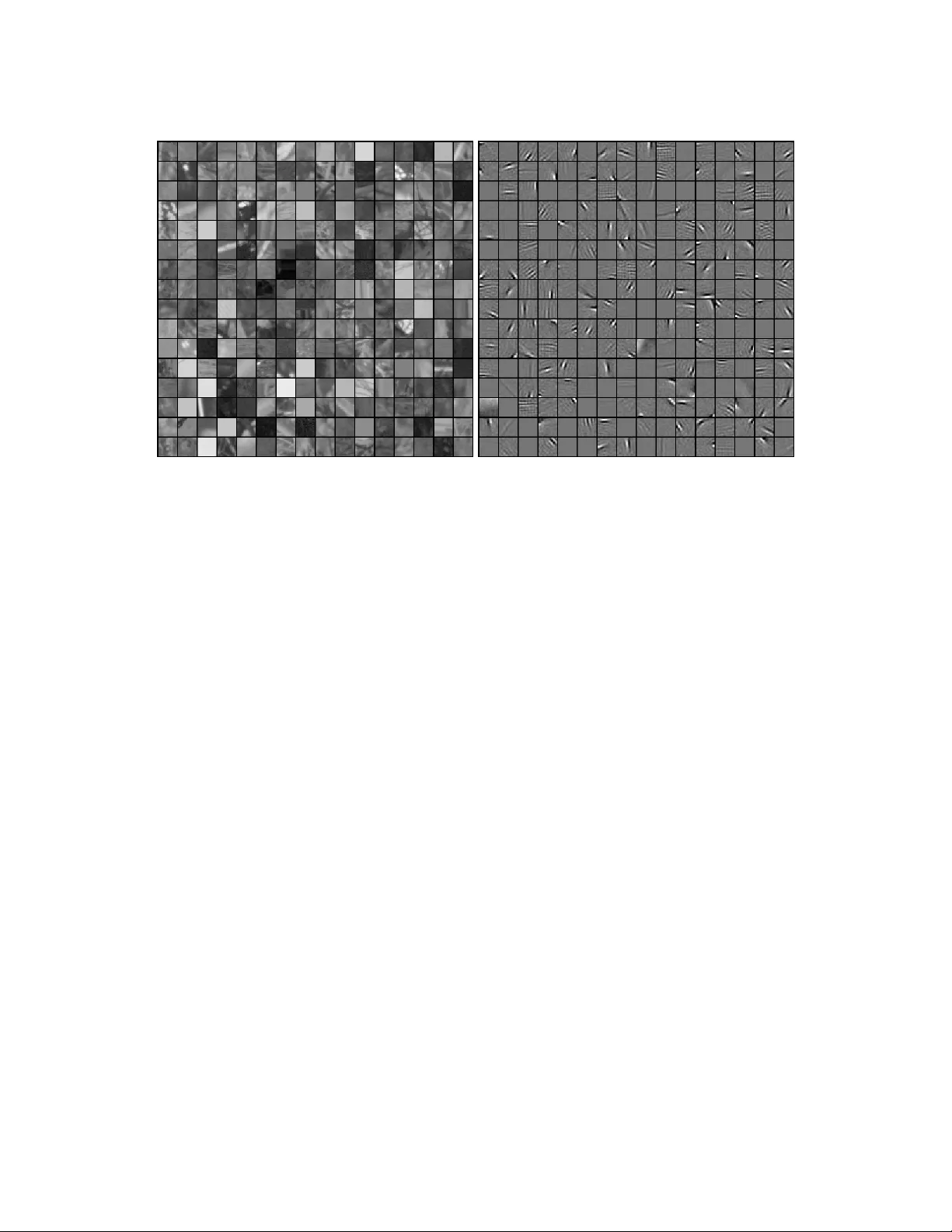
In All Lik eliho o d, Deep Belief Is Not Enough Lucas Theis, Sebastian Gerwinn, F abian Sinz and Matthias Bethge W erner Reic hardt Centre for In tegrativ e Neuroscience Bernstein Cen ter for Computational Neuroscience Max-Planc k-Institute for Biological Cyb ernetics Sp emannstraße 41, 72076 T¨ ubingen, German y { lucas,sgerwinn,fabee,mbethge } @tuebingen.mpg.de Abstract Statistical mo dels of natural stim uli pro vide an imp ortan t to ol for researc hers in the fields of machine learning and computational neuroscience. A canonical w ay to quan titatively assess and compare the performance of statistical mo dels is given by the lik eliho od. One class of statistical mo dels whic h has recently gained increasing p opularit y and has b een applied to a v ariet y of complex data are deep belief net works. Analyses of these models, ho wev er, hav e b een typically limited to qualitativ e analyses based on samples due to the computationally in tractable nature of the model likelihoo d. Motiv ated b y these circumstances, the present article pro vides a consistent estimator for the lik eliho od that is both computationally tractable and simple to apply in practice. Using this estimator, a deep b elief net work whic h has b een suggested for the mo deling of natural image patc hes is quantitativ ely in vestigated and compared to other mo dels of natural image patches. Contrary to earlier claims based on qualitative results, the results presented in this article provide evidence that the mo del under inv estigation is not a particularly go o d model for natural images. 1 In tro duction Statistical mo dels of naturally occurring stimuli constitute an important tool in machine learning and computational neuroscience, among man y other areas. In mac hine learning, they ha v e been applied both to supervised and unsup ervised problems, suc h as denoising (e.g., Lyu and Simoncelli, 2007), classification (e.g., Lee et al., 2009) or prediction (e.g., Doretto et al., 2003). In computational neuroscience, statistical models ha v e b een used to analyze the structure of natural images as part of the quest to understand the tasks faced b y the visual system of the brain (e.g., Lewicki and Doi, 2005; Olshausen and Field, 1996). Other examples include generativ e statistical mo dels studied to derive better mo dels of perceptual learning. Underlying these approac hes is the assumption that the lo w-lev el areas of the brain adapt to the statistical structure of their sensory inputs and are less concerned with goals of b eha vior. An imp ortant measure to assess the p erformance of a statistical mo del is the likelihoo d whic h allows us to ob jectiv ely compare the density estimation performance of different 1 Figure 1: L eft: Natural image patches sampled from the v an Hateren dataset (v an Hateren and v an der Sc haaf, 1998). Right: Filters learned b y a deep b elief net work trained on whitened image patc hes. mo dels. Given tw o mo del instances with the same prior probability and a test set of data samples, the ratio of their likelihoo ds already tells us everything we need to know to decide whic h of the t wo mo dels is more likely to ha ve generated the dataset. F urthermore, for densities p and ˜ p , the negative exp ected log-lik eliho o d represen ts the cr oss-entr opy (or exp e cte d lo g-loss ) term of the Kullbac k-Leibler (KL) div ergence, D KL [ ˜ p || p ] = − X x ˜ p ( x ) log p ( x ) − H [ ˜ p ] , whic h is alw ays non-negativ e and zero if and only if p and ˜ p are iden tical. The main moti- v ation for the KL-divergence stems from coding theory , where the cross-entrop y represen ts the co ding cost of enco ding samples drawn from ˜ p with a co de that w ould b e optimal for samples dra wn from p . Corresp ondingly , the KL-divergence represents the additional cod- ing cost created by using an optimal co de which assumes the distribution of the samples to b e p instead of ˜ p . Finally , the likelihoo d allows us to directly examine the success of maxi- m um likelihoo d learning for different training settings. Unfortunately , for many interesting mo dels, the lik eliho o d is in tractable to compute exactly . One such class of mo dels which has attracted a lot of atten tion in recen t y ears is given b y deep b elief net w orks. Deep belief netw orks are hierarc hical generativ e mo dels in tro duced b y Hin ton et al. (Hin ton and Salakhutdino v, 2006) together with a greedy learning rule as an approach to the long-standing challenge of training de ep neural netw orks, that is, hierarc hical neural net w orks with man y la yers. In sup ervised tasks, they hav e b een sho wn to learn represen tations whic h can b e successfully emplo yed in classification tasks, such as character recognition (Hinton et al., 2006a) and sp eech recognition (Mohamed et al., 2009). In unsup ervised tasks, where the likelihoo d is particularly imp ortant, they ha ve b een applied to a wide v ariet y of complex datasets, such as patc hes of natural images 2 (Osindero and Hinton, 2008; Ranzato et al., 2010; Ranzato and Hinton, 2010; Lee and Ng, 2007), motion capture recordings (T aylor et al., 2007) and images of faces (Susskind et al., 2008). When applied to natural images, deep b elief net works ha ve b een shown to develop biologically plausible features (Lee and Ng, 2007) and samples from the model were shown to adhere to certain statistical regularities also found in natural images (Osindero and Hin ton, 2008). Examples of natural image patches and features learned by a deep b elief net work are presen ted in Figure 1. In this article, after reviewing the relev an t asp ects of deep b elief net works, w e will de- riv e a consisten t estimator for its likelihoo d and demonstrate the estimator’s applicability in practice b y ev aluating a mo del trained on natural image patches. After a thorough quan titative analysis, w e will argue that the deep b elief netw ork under consideration is not a particularly go od mo del for estimating the densit y of small natural image patc hes, as it is outperformed with respect to the lik eliho od ev en b y simple mixture mo dels. F ur- thermore, we will show that adding lay ers to the netw ork has only a small effect on the o verall p erformance of the mo del if each la yer is trained w ell enough and will offer a p ossi- ble explanation for this observ ation by analyzing a b est-case scenario of the greedy learning pro cedure commonly used for training deep b elief net works. 2 Mo dels In this c hapter w e will review the statistical mo dels used in the remainder of this article. In particular, we will describe the restricted Boltzmann machine (RBM) and some of its v arian ts which constitute the main building blo cks for constructing deep b elief netw orks (DBNs). F urthermore, we will discuss some of the mo dels’ prop erties relev an t for estimating the likelihoo d of DBNs. Readers familiar with DBNs might wan t to skip this section or skim it to get acquainted with the notation. Throughout this article, the goal of applying statistical mo dels is assumed to b e the appro ximation of a particular distribution of interest—often called the data distribution . W e will denote this distribution b y ˜ p . 2.1 Boltzmann Mac hines A Boltzmann mac hine is a p oten tially fully connected undir e cte d gr aphic al mo del —or Markov r andom field —with binary random v ariables. Its probabilit y mass function is a Boltzmann distribution ov er 2 k binary states s ∈ { 0 , 1 } k whic h is defined in terms of an ener gy func- tion E , q ( s ) = 1 Z exp( − E ( s )) , Z = X s exp( − E ( s )) , (1) where E is given by E ( s ) = − 1 2 s > W s − b > s = − 1 2 X i,j s i w ij s j − X i s i b i (2) 3 x y (A) (B) (C) Figure 2: Boltzmann mac hines with differen t constrain ts on their connectivit y . Filled nodes denote observ ed v ariables, unfilled no des denote hidden v ariables. A: A fully con- nected latent-v ariable Boltzmann machine. B: A restricted Boltzmann machine forming a bipartite graph. C: A semi-restricted Boltzmann machine, which in con trast to RBMs also allows connections b et ween the visible units. and dep ends on a symmetric w eight matrix W ∈ R k × k with zeros on the diagonal, i.e. w ii = 0 for all i = 1 , ..., k , and bias terms b ∈ R k . Z is called p artition function and ensures the normalization of q . In the following, unnormalized distributions will b e marked with an asterisk: q ∗ ( s ) = Z q ( s ) = exp( − E ( s )) . Samples from the Boltzmann distribution can b e obtained via Gibbs sampling , whic h op- erates b y conditionally sampling each univ ariate random v ariable un til some conv ergence criterion is reached. F rom definitions (1) and (2) it follows that the conditional probability of a unit i b eing on given the states of all other units s j 6 = i is given by q ( s i = 1 | s j 6 = i ) = g   X j w ij s j + b i   , where g ( x ) = 1 / (1 + exp( − x )) is the sigmoidal logistic function. The Boltzmann machine can be seen as a sto c hastic generalization of the binary Hopfield netw ork, whic h is based on the same energy function but up dates its units deterministically using a step function, i.e. a unit is set to 1 if P j w ij s i + b i > 0 and set to 0 otherwise. In the limit of increasingly large w eigh t magnitudes, the logistic function b ecomes a step function and the deterministic b eha vior of the Hopfield netw ork can be reco vered with the Boltzmann mac hine (Hin ton, 2007). Of particular in terest for building DBNs are latent variable Boltzmann machines , that is, Boltzmann machines for whic h the states s are only partially observ ed (Figure 2). W e will refer to states of observed—or visible—random v ariables as x and to states of unobserv ed— or hidden—random v ariables as y , suc h that s can b e written as s = ( x, y ). Appro ximation of the data distribution ˜ p ( x ) with the mo del distribution q ( x ) via max- im um likelihoo d (ML) learning can b e implemen ted by following the gradient of the mo del log-lik eliho o d. In Boltzmann mac hines, this gradien t is conceptually simple yet computa- tionally very hard to ev aluate. The gradient of the exp ected log-lik eliho od with respect to 4 some parameter θ of the energy function is (Salakh utdino v, 2009): E ˜ p ( x )  ∂ ∂ θ log q ( x )  = E q ( x,y )  ∂ ∂ θ E ( x, y )  − E ˜ p ( x ) q ( y | x )  ∂ ∂ θ E ( x, y )  . (3) The first term on the right-hand side of this equation is the exp ected gradient of the energy function when b oth hidden and observed states are sampled from the mo del, while the second term is the exp ected gradien t of the energy function when the hidden states are dra wn from the conditional distribution of the mo del, given a visible state drawn from the data distribution. F ollowing this gradient increases the energy of the states which are more lik ely with respect to the model distribution and decreases the energy of the states whic h are more likely with resp ect to the data distribution. Remember that b y the definition of the mo del (1), states with higher energy are less likely than states with low er energy . As an example, the gradient of the log-likelihoo d with resp ect to the weigh t connecting a visible unit x i and a hidden unit y j b ecomes E ˜ p ( x ) q ( y | x ) [ x i y j ] − E q ( x,y ) [ x i y j ] . A step in the direction of this gradient can b e interpreted as a com bination of Hebbian and an ti-Hebbian learning (Hinton, 2003), where the first term corresp onds to Hebbian learning and the second term to anti-Hebbian learning, resp ectiv ely . Ev aluating the expectations, ho wev er, is computationally intractable for all but the simplest net w orks. Even appro ximating the expectations with Mon te Carlo methods is t ypically v ery slo w (Long and Serv edio, 2010). Two measures can b e tak en to mak e learning in Boltzmann mac hines feasible: constraining the Boltzmann mac hine in some w ay , or replacing the lik eliho o d with a simpler ob jectiv e function. The former approac h led to the in tro duction of RBMs, which will b e discussed in the next section. The latter approach led to the no w widely used contrastiv e divergence (CD) learning rule (Hinton, 2002) whic h represen ts a tractable appro ximation to ML learning: In CD learning, the exp ectation ov er the mo del distribution q ( x, y ) is replaced by an expectation o ver q CD ( x, y ) = X x 0 ,y 1 ˜ p ( x 0 ) q ( y 1 | x 0 ) q ( x | y 1 ) q ( y | x ) , from whic h samples are obtained by taking a sample x 0 from the data distribution, updating the hidden units, updating the visible units, and finally updating the hidden units again, while in eac h step k eeping the resp ectiv e set of other v ariables fixed. This corresponds to a single sw eep of Gibbs sampling through all random v ariables of the mo del plus an additional up date of the hidden units. If instead n sw eeps of Gibbs sampling are used, the learning procedure is generally referred to as CD( n ) learning. F or n → ∞ , ML learning is regained (Salakhutdino v, 2009). 2.2 Restricted Boltzmann Machines A restricted Boltzmann machine (RBM) (Smolensky, 1986) is a Boltzmann machine whose energy function is constrained such that no direct in teraction be t w een t wo visible units or t wo hidden units is p ossible, E ( x, y ) = − x > W y − b > x − c > y . 5 The corresp onding graph has no connections b etw een the visible units and no connections b et w een the hidden units and is hence bipartite (Figure 2). The weigh t matrix W ∈ R m × n is differen t to the one in equation (2) in that it now only con tains in teraction terms b et ween the m visible units and the n hidden units and therefore no longer needs to b e symmetric or constrained in any other w ay . Despite these constraints it has been shown that RBMs are univ ersal appro ximators, i.e. for any distribution ov er binary states and an y ε > 0, there exists an RBM with a KL-divergence whic h is smaller than ε (Roux and Bengio, 2008). In an RBM, the visible units are conditionally indep enden t giv en the states of the hidden units and vice versa. The conditional distribution of the hidden units, for instance, is giv en b y q ( y | x ) = Y j q ( y j | x ) , q ( y j | x ) = g ( w > j x + c j ) , where g is the logistic sigmoidal function and w j is the j -th column of W . This allows for efficient Gibbs sampling of the mo del distribution (since one set of v ariables can b e up dated in parallel giv en the other) and thus for faster approximation of the log-lik eliho o d gradien t. Moreov er, the unnormalized marginal distributions q ∗ ( x ) and q ∗ ( y ) of RBMs can b e computed analytically by in tegrating out the resp ectiv e other v ariable. F or instance, the unnormalized marginal distribution of the visible units b ecomes q ∗ ( x ) = exp( b > x ) Y j (1 + exp( w > j x + c j )) . (4) Tw o other mo dels whic h can b e used for constructing DBNs are the Gaussian RBM (GRBM) (Salakh utdinov, 2009) and the semi-r estricte d Boltzmann machine (SRBM) (Osindero and Hin ton, 2008). The GRBM employs cont inuous instead of binary visible units (while keep- ing the hidden units binary) and can th us b e used to model con tinuous data. Its energy function is given b y E ( x, y ) = 1 2 σ 2 || x − b || 2 − 1 σ x > W y − c > y . (5) A somewhat more general definition allows a differen t σ for each individual visible unit (Salakh utdinov, 2009). As for the binary Boltzmann machine, training of the GRBM pro- ceeds by following the gradien t given in equation (3), or an appro ximation thereof. Its prop erties are similar to that of an RBM, except that its conditional distribution q ( x | y ) is a multiv ariate Gaussian distribution whose mean is determined by the hidden units, q ( x | y ) = N ( x ; W y + b, σ I ) . Eac h state of the hidden units enco des one mean. σ controls the v ariance of each Gaussian and is the same for all states of the hidden units. The GRBM can therefore b e in terpreted as a mixture of an exp onen tial num b er of Gaussian distributions with fixed, isotropic co- v ariance and parameter sharing constraints. In an SRBM, only the hidden units are constrained to ha ve no direct connections to eac h other while the visible units are unconstrained (Figure 2). Imp ortan tly , analytic expressions are therefore only av ailable for q ∗ ( x ) but not for q ∗ ( y ). F urthermore, q ( x | y ) is no longer 6 factorial. F or efficiently training DBNs, conditional indep endence of the hidden units is more imp ortan t than conditional indep endence of the visible units (Osindero and Hinton, 2008). This is in part due to the fact that the second-term on the right-hand side of equation (3) can still efficiently b e ev aluated if the hidden units are conditionally independent, and in part due to the wa y inference is done in DBNs. 2.3 Deep Belief Netw orks x y z Figure 3: A graphical mo del representation of a tw o-la yer deep b elief net work comp osed of t wo RBMs. Note that the connections of the first la yer are directed. DBNs (Hin ton and Salakh utdinov, 2006) are hierarchical generative mo dels comp osed of sev eral lay ers of RBMs or one of their generalizations. While DBNs ha ve been widely used as part of a heuristic for learning m ultiple la yers of feature representations and for pretraining multi-la y er perceptrons (b y initializing the multi-la y er p erceptron with the pa- rameters learned by a DBN), the existence of an efficien t learning rule has made them b ecome attractive also for densit y estimation tasks. F or simplicit y , w e will b egin by defining a t wo-la y er DBN. Let q ( x, y ) and r ( y , z ) b e the densities of t wo RBMs o ver visible states x and hidden states y and z . Then, the join t probabilit y mass function of a t wo-la y er DBN is defined to b e p ( x, y , z ) = q ( x | y ) r ( y , z ) . (6) In terestingly , the resulting distribution is b est describ ed not as a deep Boltzmann machine, as one migh t expect, or ev en an undirected graphical mo del, but as a graphical mo del with undirected connections b et ween y and z and directed connections b etw een x and y (Figure 3). This characteristic of the mo del b ecomes eviden t in the generative pro cess. A sample from the mo del can b e dra wn b y first Gibbs sampling the distribution r ( y , z ) of the top lay er to produce a state for y . Afterw ards, a sample is dra wn from the muc h simpler distribution q ( x | y ). The definition can easily be extended to DBNs with three or more la yers b y replacing r ( y, z ) = r ( y | z ) r ( z ) with r ( y | z ) s ( z ), where s ( z ) is the marginal distribution of another RBM. Thus, by adding additional lay ers to the DBN, the prior distribution ov er the top-lev el hidden units— r ( z ) for the mo del defined in equation (6)—is effectively replaced with a new prior distribution—in this case s ( z ). DBNs with an arbitrary num b er of lay ers, like RBMs, ha ve b een sho wn to be univ ersal approximators even if the num b er of hidden units in each 7 la yer is fixed to the n umber of visible units (Sutskev er and Hinton, 2008). As mentioned earlier, another p ossibilit y to generalize DBNs is to allow for more general mo dels as lay ers. One suc h mo del is the SRBM, which can model more complex interactions b y having less restrictiv e indep endce assumptions. Alternativ ely , one could allow for mo dels with units whose conditional probability distributions are not just binary , but can b e any exp onen tial family distribution (W elling et al., 2005)—one instance being the GRBM. The greedy learning pro cedure (Hinton et al., 2006a) used for training DBNs starts b y fitting the first-la yer RBM (the one closest to the observ ations) to the data distribution. Afterw ards, the prior distribution o v er the hidden units defined by the first lay er, q ( y ) = P x q ( x, y ), is replaced b y the marginal distribution of the second lay er, r ( y ), and the parameters of the second la y er are trained b y optimizing a lo wer b ound to the log-lik eliho o d of the tw o-lay er DBN. In the follo wing, w e will deriv e this lo w er bound. Let θ b e a parameter of r . The gradient of the log-lik eliho od with resp ect to θ is ∂ ∂ θ log p ( x ) = 1 p ( x ) X y ∂ ∂ θ p ( x, y ) = 1 p ( x ) X y p ( x, y ) ∂ ∂ θ log p ( x, y ) = X y p ( y | x ) ∂ ∂ θ log( r ( y ) q ( x | y )) = X y p ( y | x )     ∂ ∂ θ log r ( y ) + ∂ ∂ θ log q ( x | y ) | {z } = 0     = X y p ( y | x ) ∂ ∂ θ log r ( y ) . (7) Appro ximate ML learning could therefore in principle be implemented by training the sec- ond lay er to appro ximate the posterior distribution p ( y | x ) using CD learning or a similar algorithm. How ev er, exact sampling from the p osterior distribution p ( y | x ) is difficult, as its ev aluation inv olv es integrating o ver an exp onen tial num ber of states, p ( y | x ) = p ( x, y ) p ( x ) = q ( x | y ) r ( y ) P y q ( x | y ) r ( y ) . In order to make the training feasbile again, the p osterior distribution is replaced b y the factorial distribution q ( y | x ). T raining the DBN in this manner optimizes a v ariational lo wer b ound on the log-likelih o o d, log p ( x ) = log X y q ( x | y ) r ( y ) = log X y q ( y | x ) q ( x ) q ( y ) r ( y ) (8) ≥ X y q ( y | x ) log r ( y ) + const, (9) 8 where (8) follows from Bay es’ theorem, (9) is due to Jensen’s inequality and const is constant in θ , as only r dep ends on θ . T aking the deriv ative of (9) with respect to θ yields (7) with the p osterior distribution p ( y | x ) replaced by q ( y | x ). The greedy learning procedure can b e generalized to more lay ers by training each additional lay er to approximate the distribution obtained by conditionally sampling from each lay er in turn, starting with the lo west la yer. 3 Lik eliho o d Estimation In this section, we will discuss the problem of estimating the likelihoo d of a tw o-la yer DBN with joint density p ( x, y , z ) = q ( x | y ) r ( y , z ) . (10) That is, for a given visible state x , to estimate the v alue of p ( x ) = X y ,z q ( x | y ) r ( y, z ) . As w e will see later, this problem can easily be generalized to more la y ers. As b efore, q ( x, y ) and r ( y , z ) refer to the densities of t wo RBMs. Tw o difficulties arise when dealing with this problem in the context of DBNs. First, r ( y, z ) dep ends on a partition function Z r whose exact ev aluation requires integration ov er an exponential n um b er of states. Second, despite our ability to in tegrate analytically o ver z , even computing just the unnormalized lik eliho o d still requires in tegration o ver an exp o- nen tial n um b er of hidden states y , p ∗ ( x ) = X y q ( x | y ) r ∗ ( y ) . After briefly reviewing previous approac hes to resolving these difficulties, w e will prop ose an un biased estimator for p ∗ ( x ), its contribution b eing a possible solution to the second prob- lem, and discuss ho w to construct a consistent estimator for p ( x ) based on this estimator. Finally , we will demonstrate its applicability to more general DBNs. 3.1 Previous W ork 3.1.1 Annealed Importance Sampling Salakh utdinov and Murra y (2008) hav e shown how anne ale d imp ortanc e sampling (AIS) (Neal, 2001) can b e used to estimate the partition function of a restricted Boltzmann ma- c hine. Since our estimator will also rely on AIS estimates of the partition function, we will shortly describ e the pro cedure here. Imp ortance sampling is a Mon te Carlo method for unbiased estimation of exp ectations (MacKa y, 2003) and is based on the following observ ation: Let s be a density with s ( x ) > 0 whenev er q ∗ ( x ) > 0 and let w ( x ) = q ∗ ( x ) s ( x ) , then X x q ∗ ( x ) f ( x ) = X x s ( x ) q ∗ ( x ) s ( x ) f ( x ) = E s ( x ) [ w ( x ) f ( x )] (11) 9 for an y function f ( x ). s is called the pr op osal distribution and w ( x ) is called imp ortanc e weight . F or f ( x ) = 1, we get E s ( x ) [ w ( x )] = X x s ( x ) q ∗ ( x ) s ( x ) = Z q . (12) Estimates of the partition function Z q can therefore b e obtained b y dra wing samples x ( n ) from a prop osal distribution and a veraging the resulting imp ortance w eights w ( x ( n ) ). It w as p oin ted out in (Mink a, 2005) that minimizing the v ariance of the im portance sampling estimate of the partition function (12) is equiv alent to minimizing an α -div ergence 1 b et w een the prop osal distribution s and the true distribution q . Therefore, for the estimate to w ork w ell in practice, s should b e b oth close to q and easy to sample from. Annealed importance sampling (Neal, 2001) tries to circum ven t some of the problems asso ciated with finding a suitable prop osal distribution. Assume we can construct a distri- bution s 1 whic h approximates q well, but which is still difficult to sample from or whic h w e can only ev aluate up to a normalization factor. Let s 2 b e another distribution. This distri- bution will effectiv ely act as a prop osal distribution for s 1 . F urther, let T 1 b e a tr ansition op er ator which lea v es the distribution of s 1 in v ariant, i.e. let T 1 ( x 0 ; x 1 ) b e a probabilit y distribution ov er x 0 dep ending on x 1 , such that s 1 ( x 0 ) = X x 1 s 1 ( x 1 ) T 1 ( x 0 ; x 1 ) . W e then ha ve Z q = X x 0 s 1 ( x 0 ) q ∗ ( x 0 ) s 1 ( x 0 ) = X x 0 X x 1 s 1 ( x 1 ) T 1 ( x 0 ; x 1 ) q ∗ ( x 0 ) s 1 ( x 0 ) = X x 0 X x 1 s 2 ( x 1 ) T 1 ( x 0 ; x 1 ) s ∗ 1 ( x 1 ) s 2 ( x 1 ) q ∗ ( x 0 ) s ∗ 1 ( x 0 ) . Note that we don’t hav e to know the partition function of s 1 to ev aluate the right-hand term. Also note that we don’t need to sample from s 1 but only from T 1 if we wan t to estimate this term via Monte Carlo in tegration. If s 2 is still to o difficult to handle, we can apply the same trick again by introducing a third distribution s 3 and a transition op erator T 2 for s 2 . By induction, w e can see that Z q = X x s n ( x n − 1 ) T n − 1 ( x n − 2 ; x n − 1 ) · · · T 1 ( x 0 ; x 1 ) s ∗ n − 1 ( x n − 1 ) s n ( x n − 1 ) · · · q ∗ ( x 0 ) s ∗ 1 ( x 0 ) , where the sum integrates ov er all x = ( x 0 , ..., x n − 1 ). Hence, in order to estimate the partition function, w e can draw indep endent samples x n − 1 from a simple distribution s n , use the transition op erators to generate intermediate samples x n − 2 , ..., x 0 , and use the product of fractions in the preceding equation to compute imp ortance w eights, which w e then av erage. 1 With α = 2. α -divergences are a generalization of the KL-div ergence. 10 In order to b e able to apply AIS to RBMs, a sequence of intermediate distributions and corresp onding anne aling weights is defined: s ∗ k ( x ) = q ∗ ( x ) 1 − β k s ( x ) β k , β k ∈ [0 , 1] for k = 0 , ..., n , where β 0 = 0 and β n = 1. If w e also choose an RBM for s , then s k is itself a Boltzmann distribution whose energy function is a weigh ted sum of the energy functions of s and q . Similarly , natural and efficien t implementations based on Gibbs sampling can b e found for the transition op erators T k . 3.1.2 Estimating Lo wer Bounds In (Salakhutdino v and Murray, 2008) it was also shown how estimates of a low er b ound on the log-likelihoo d, log p ( x ) ≥ X y q ( y | x ) log r ∗ ( y ) q ( x | y ) q ( y | x ) − log Z r (13) = X y q ( y | x ) log r ∗ ( y ) q ( x | y ) + H [ q ( y | x )] − log Z r , (14) can b e obtained, provided the partition function Z r is given. This is the same lo wer b ound as the one optimized during greedy learning (9). Since q ( y | x ) is factorial, the en tropy H [ q ( y | x )] can b e computed analytically . The only term whic h still needs to be estimated is the first term on the righ t-hand side of equation (14). This w as ac hieved in (Salakhutdino v and Murray, 2008) b y drawing samples from q ( y | x ). 3.1.3 Consisten t Estimates In (Murray and Salakh utdinov, 2009), carefully designed Mark ov chains w ere constructed to giv e unbiased estimates for the in verse p osterior probability 1 p ( y | x ) of some fixed hidden state y . These estimates were then used to get un biased estimates of p ∗ ( x ) by taking adv antage of the fact p ∗ ( x ) = p ∗ ( x,y ) p ( y | x ) . The corresp onding partition function was estimated using AIS, leading to an ov erall estimate of the lik eliho o d that tends to ov erestimate the true lik eliho od. While the estimator w as constructed in suc h a w ay that even v ery short runs of the Marko v chain result in un biased estimates of p ∗ ( x ), even a single step of the Mark ov chain is slow compared to sampling from q ( y | x ) as it was done for the estimation of the low er b ound (13). 3.2 A New Estimator for DBNs The estimator w e will in tro duce in this section shares the same formal prop erties as the estimator prop osed in (Murra y and Salakhutdino v, 2009), but will utilize samples drawn from q ( y | x ). This will make it conceptually as simple and as easy to apply in practice as the estimator for the lo wer bound (13), while pro viding us with consisten t estimates of p ( x ). 11 3.2.1 Definition Let p ( x, y , z ) b e the joint density of a DBN as defined in equation (10). By applying Bay es’ theorem, we obtain p ( x ) = X y q ( x | y ) r ( y ) (15) = X y q ( y | x ) q ( x ) q ( y ) r ( y ) (16) = X y q ( y | x ) q ∗ ( x ) q ∗ ( y ) r ∗ ( y ) Z r . (17) An obvious choice for an estimator of p ( x ) is then ˆ p N ( x ) = 1 N X n q ∗ ( x ) q ∗ ( y ( n ) ) r ∗ ( y ( n ) ) Z r (18) = q ∗ ( x ) 1 Z r N X n r ∗ ( y ( n ) ) q ∗ ( y ( n ) ) (19) where y ( n ) ∼ q ( y ( n ) | x ) for n = 1 , ..., N . F or RBMs, the unnormalized marginals q ∗ ( x ) , q ∗ ( y ) and r ∗ ( y ) can b e computed analytically (4). Note that the partition function Z r only has to b e calculated once for all visible states we wish to ev aluate. Intuitiv ely , the estimation pro cess can be imagined as first assigning a basic v alue to x using the distribution of the first lay er, and then with ev ery sample adjusting this v alue dep ending on ho w the second la yer distribution relates to the first la yer distribution. 3.2.2 Prop erties Under the assumption that the partition function Z r is kno wn, ˆ p ( x ) pro vides an unbiased estimate of p ( x ) since the sample av erage is alwa ys an un biased estimate of the exp ectation. Ho wev er, Z r is generally intractable to compute exactly s o that approximations b ecome necessary . In fact, in (Long and Servedio, 2010) it w as sho wn that already approximating the partition function of an RBM to within a multiplicativ e factor is generally NP-hard in the num b er of parameters of the RBM. If in the estimate (18), Z r is replaced b y an unbiased estimate ˆ Z r , then the ov erall estimate will tend to ov erestimate the true likelihoo d, E  ˆ p ∗ N ( x ) ˆ Z r  = E  1 ˆ Z r  E [ ˆ p ∗ N ( x )] ≥ 1 E h ˆ Z r i p ∗ ( x ) = p ( x ) , where ˆ p ∗ N ( x ) = Z r ˆ p N ( x ) is an unbiased estimate of the unnormalized density . The second step is a consequence of Jensen’s inequalit y and the a verages are tak en with resp ect to ˆ p N ( x ) and ˆ Z r , which are independent; x is held fix. 12 While the estimator loses its unbiasedness for un biased estimates of the partition func- tion, it still retains its consistency . Since p ∗ N ( x ) is un biased for all N ∈ N , it is also asymptotically unbiased, plim N →∞ p ∗ N ( x ) = p ∗ ( x ) . F urthermore, if ˆ Z r,N for N ∈ N is a consistent sequence of estimators for the partition function, it follows that plim N →∞ ˆ p ∗ N ( x ) ˆ Z r,N = plim N →∞ ˆ p ∗ N ( x ) plim N →∞ ˆ Z r,N = p ∗ ( x ) Z r = p ( x ) . Un biased and consistent estimates of Z r can b e obtained using AIS (Salakh utdinov and Murra y, 2008). Note that although the estimator tends to ov erestimate the true likelihoo d in expectation and is unbiased in the limit, it is still p ossible for it to underestimate the true likelihoo d most of the time. This b eha vior can o ccur if the distribution of estimates is hea vily sk ew ed. Another question which remains is whether the estimator is go od in terms of efficiency , or in other w ords: Ho w many samples are required b efore a reliable estimate of the true lik eliho o d is ac hieved? T o address this question, we reform ulate the exp ectation in equation (17) to give p ( x ) = X y q ( y | x ) p ( x, y ) q ( y | x ) . In this form ulation it becomes eviden t that estimating p ( x ) is equiv alent to estimating the partition function of p ( y | x ) using imp ortance sampling. T o see this, notice that, for a fixed x , p ( x, y ) is just an unnormalized v ersion of p ( y | x ), where p ( x ) is the normalization constan t, p ( y | x ) = p ( x, y ) p ( x ) . The prop osal distribution in this case is q ( y | x ). As mentioned earlier, the efficiency of imp ortance sampling estimates dep ends on ho w w ell the proposal distribution appro ximates the true distribution. Therefore, for the prop osed estimator to w ork w ell in practice, q ( y | x ) should b e close to p ( y | x ). Note that a similar assumption is made when optimizing the v ariational low er b ound (9) during greedy learning. 3.2.3 Generalizations The definition of the estimator for t wo-la yer DBNs readily extends to DBNs with L la yers. If p ( x ) is the marginal density of a DBN whose lay ers are constituted by RBMs with densities q 1 , ..., q L and partition fun ctions Z 1 , ..., Z L , and if w e refer to the states of the random 13 v ectors in eac h lay er by x 0 , ..., x L , where x 0 con tains the visible states and x L con tains the states of the top hidden lay er, then p ( x 0 ) = X x 1 ,...,x L − 1 q L ( x L − 1 ) L − 1 Y l =1 q l ( x l − 1 | x l ) = X x 1 ,...,x L − 1 q L ( x L − 1 ) L − 1 Y l =1 q l ( x l | x l − 1 ) q ∗ l ( x l − 1 ) q ∗ l ( x l ) = q ∗ 1 ( x 0 ) 1 Z L X x 1 ,...,x L − 1 L − 1 Y l =1 q l ( x l | x l − 1 ) q ∗ l +1 ( x l ) q ∗ l ( x l ) . In order to estimate this term, hidden states x 1 , ..., x L are generated in a feed-forw ard manner using the conditional distributions q l ( x l | x l − 1 ). The weigh ts q ∗ l +1 ( x l ) q ∗ l ( x l ) are computed along the wa y , then m ultiplied together and finally av eraged o ver all dra wn states. Often, a DBN not only contains RBMs but also more general distributions q ( x, y ) (see, for example, Roux et al., 2010; Osindero and Hinton, 2008; Ranzato et al., 2010; Ranzato and Hin ton, 2010). In this case, analytical expressions of the unnormalized distribution o ver the hidden states q ∗ ( y ) might b e unav ailable, as, for example, for the SRBM. If AIS or some other imp ortance sampling metho d is used for the estimation of the partition function, ho wev er, the same imp ortance samples and imp ortance weigh ts can b e used in order to get un biased estimates of q ∗ ( y ), as we will show in the following. As in equation (11), let s b e a prop osal distribution and w b e imp ortance weigh ts such that X x s ( x ) w ( x ) f ( x ) = X x q ∗ ( x ) f ( x ) . for an y function f . By noticing that q ∗ ( y ) = P x q ∗ ( x ) q ( y | x ), it easy to see how estimates of q ∗ ( y ) can b e obtained using the same imp ortance samples and imp ortance weigh ts which are used for estimating the partition function, q ∗ ( y ) ≈ 1 N X n w ( n ) q ( y | x ( n ) ) . As for the partition function, the imp ortance w eights only hav e to b e generated once for all x and all hidden states that are part of the ev aluation. Estimating q ∗ ( y ) in this manner, ho wev er, in tro duces further bias into the estimator. Also note that a go od prop osal distri- bution for estimating the partition function need not b e a go o d proposal distribution for estimating the marginals. The optimal proposal distribution for estimating the marginals w ould be q ( x ), as in this case an y importance w eigh t w ould tak e on the v alue of the par tition function itself (12). The optimal proposal distribution for estimating the v alue of the un- normalized marginal distribution q ∗ ( y ), on the other hand, is q ( x | y ), which unfortunately dep ends on y . Therefore, more imp ortance samples will b e needed in order to get reliable estimates of the marginals. 14 3.3 P oten tial L og-Lik eliho o d In this section, we will discuss the concept of the p otential lo g-likeliho o d —a concept which app ears in (Roux and Bengio, 2008). By considering a b est-case scenario, the potential log-lik eliho o d giv es an idea of the log-lik eliho o d that can at b est be achiev ed by training additional la yers using greedy learning. Its usefulness will b ecome apparen t in the exp eri- men tal section. Let q ( x, y ) b e the distribution of an already trained RBM or one of its generalizations, and let r ( y ) b e a second distribution—not necessarily the marginal distribution of an y Boltz- mann machine. As in section 2.3, r ( y ) serv es to replace the prior distribution ov er the hidden v ariables, q ( y ), and thereb y impro ve the marginal distribution o ver x , P y q ( x | y ) r ( y ). As ab o v e, let ˜ p ( x ) denote the data distribution. Our goal, then, is to increase the exp ected log-lik eliho o d of the mo del distribution with respect to r , X x ˜ p ( x ) log X y q ( x | y ) r ( y ) . (20) In applying the greedy learning pro cedure, w e try to reach this goal by optimizing a lo wer b ound on the log-lik eliho o d (9), or equiv alently , b y minimizing the follo wing KL-div ergence: D KL " X x ˜ p ( x ) q ( y | x ) || r ( y ) # = − X x ˜ p ( x ) X y q ( y | x ) log r ( y ) + const, where c onst is constant in r . The KL divergence is minimal if r ( y ) is equal to X x ˜ p ( x ) q ( y | x ) (21) for ev ery y . Since RBMs are universal approximators (Roux and Bengio, 2008), this dis- tribution could in principle b e appro ximated arbitrarily w ell b y a single, pote n tially very large RBM (provided the y are binary). Assume that w e ha ve found this distribution, that is, we hav e maximized the lo wer b ound with resp ect to all p ossible distributions r . The distribution for the DBN whic h we obtain by replacing r in (20) with (21) is then giv en by X y q ( x | y ) X x 0 ˜ p ( x 0 ) q ( y | x 0 ) = X x 0 ˜ p ( x 0 ) X y q ( x | y ) q ( y | x 0 ) = X x 0 ˜ p ( x 0 ) q 0 ( x | x 0 ) , where we hav e used the r e c onstruction distribution q 0 ( x | x 0 ) = X y q ( x | y ) q ( y | x 0 ) , whic h can be sampled from b y conditionally sampling a state for the hidden units, and then, giv en the state of the hidden units, conditionally sampling a r e c onstruction of the visible 15 1 2 3 space of distributions r [bits] log-lik eliho o d lo wer b ound Figure 4: A carto on explaining the potential log-likelihoo d. The p oten tial log-likelihoo d is the log-lik eliho o d ev aluated at (2), where the lo wer b ound reac hes its optim um (1). This does not exclude the existence of a distribution r for whic h the log-lik eliho o d is larger than the p oten tial log-lik eliho o d, as in (3), but it is unlik ely that this p oin t will b e found b y greedy learning, which optimizes r only with resp ect to the low er b ound. units. The log-lik eliho o d we achiev e with this low er-b ound optimal distribution is given by X x ˜ p ( x ) log X x 0 ˜ p ( x 0 ) q 0 ( x | x 0 ) . (22) w e will refer to this log-likelihoo d as the p otential lo g-likeliho o d (and to the corresp onding log-loss as the p otential lo g-loss ). Note that the p oten tial log-likelihoo d is not a true upp er b ound on the log-likelihoo d that can b e achiev ed with greedy learning, as sub optimal solu- tions with resp ect to the low er bound migh t still giv e rise to higher log-likelihoo ds. How ev er, if suc h a solution was found, it w ould ha ve rather b een by acciden t than b y design. The situation is depicted in the carto on in Figure 4. 4 Exp erimen ts In order to test the estimator, we considered the task of modeling 4x4 natural image patc hes sampled from the v an Hateren dataset (v an Hateren and v an der Schaaf, 1998). W e chose a small patc h size to allow for a more thorough analysis of the estimator’s b eha vior and the effects of certain mo del parameters. In all exp eriments, a standard battery of prepro cessing steps w as applied to the image patc hes, including a log-transformation, a centering step and a whitening step. Additionally , the DC comp onen t w as pro jected out and only the other 15 comp onen ts of each image patch were used for training (for details, see Eichhorn et al., 2009). In (Osindero and Hinton, 2008), a three-lay er DBN based on GRBMs and SRBMs was suggested for the mo deling of natural image patches. The mo del emplo yed a GRBM in the 16 la yers true avg. log-loss est. a vg. log-loss 1 2.0550777 2.0551289 2 2.0550775 2.0550734 3 2.0550773 2.0544256 T able 1: T rue and estimated log-loss of a small-scale v ersion of the mo del. Adding more la yers to the netw ork does not help to improv e the p erformance if the GRBM emplo ys only few hidden units. first la yer and SRBMs in the second and third la yer. In contrast to samples from the same mo del without lateral connections, samples from the prop osed mo del w ere shown to possess some of the statistical regularities also found in natural images, such as sparse distributions of pixel intensities and the right pair-wise statistics of Gab or filter resp onses. F urthermore, the first la yer of the mo del w as shown to dev elop oriented edge filters (Figure 1). In the follo wing, w e will further analyse this type of mo del by estimating its lik eliho o d. F or training and ev aluation, w e used 10 indep enden t pairs of training and test sets con- taining 50000 samples each. W e trained the mo dels using the greedy learning pro cedure describ ed in Section 2.3. The scale-parameter σ of the GRBM (5) w as chosen via cross- v alidation. After training a GRBM, we initialized the second-lay er SRBM such that its visible marginal distribution is equal to the hidden marginal distribution of the GRBM. Initializing the second la yer in this manner has the follo wing adv antages. First, after ini- tialization, the likelihoo d of the t wo-la y er DBN consisting of the trained GRBM and the initialized SRBM is equal to the likelihoo d of the GRBM. Second, the lo wer b ound on the DBN’s log-likelihoo d (9) is equal to its actual log-lik eliho o d. Using the notation of the previous sections: r ( y ) = q ( y ) ⇒ X y q ( y | x ) log  r ( y ) q ( x ) q ( y )  = log p ( x ) . As a consequence, an impro vemen t in the low er b ound necessarily leads to an improv ement in the log-likelihoo d (Salakhutdino v, 2009). All trained mo dels w ere ev aluated using the prop osed estimator. W e used AIS in order to estimate the partition functions and the marginals of the SRBMs. Performances w ere measured as av erage log-loss in bits and normalized b y the num b er of comp onen ts. Details on the training and ev aluation parameters can b e found in App endix A. 4.1 Small Scale Exp eriment In a first exp erimen t, we in vestigated a small-scale version of the mo del for whic h the lik eliho o d is still tractable. It employ ed 15 hidden units in the first lay er, 15 hidden units in the second lay er and 50 hidden units in the third lay er, where each la yer was trained for 50 ep o c hs using CD(1). Brute-force and estimated results are given in T able 1. A first observ ation whic h can b e made is that the estimated performance is v ery close to the true p erformance. Another observ ation is that the second and third lay er do not help to impro ve the performance of the mo del, which hints at the fact that the 15 hidden 17 10 0 10 1 10 2 10 3 0 0 . 5 1 1 . 5 2 n umber of AIS samples log-loss [bits] estimating marginals estimating partition fct. true av erage log-loss 10 2 10 3 10 4 10 5 0 0 . 5 1 1 . 5 2 n umber of AIS samples log-loss [bits] Figure 5: L eft: A small-scale DBN was ev aluated while either only estimating the parti- tion function of the third-la yer SRBM (orange curv e) or estimating the hidden marginal distribution of the second-lay er SRBM (blue curv e), while using differen t n umbers of AIS samples. The parameters of the AIS pro cedure w ere the same for b oth estimates. In particular, the same num b er of in termediate annealing distributions was used. Unsurprisingly , the estimated log-loss is more sensitive to the n umber of samples used for estimating the marginals. Right: The graph sho ws the estimated performance of DBN-100 while changing the num b er of im- p ortance samples used to estimate the marginals of the second-lay er SRBM. The plot indicates that the true log-loss is still sligh tly larger than the estimates we obtained even after taking 10 5 samples. units of the GRBM are unable to capture muc h of the information in the contin uous visible units. In order to ev aluate the lik eliho o d of this model using the proposed estimator, the un- normalized marginals of the second-lay er SRBM’s hidden units with resp ect to the SRBM as well as the partition function of the third lay er SRBM had to b e estimated. W e inv esti- gated the effect of the n umber of imp ortance samples used in b oth estimates on the ov erall estimate of the log-loss and made the following observ ations. First, almost no error could b e observed in the estimates of the partition function—and hence of the log-loss—ev en if just one imp ortance sample was used (left plot in Figure 5). This is the case if the prop osal distribution is very close to the true distribution, as can b e seen from equation (12) by replacing the former with the latter. How ev er, the reason for this observ ation is likely to b e found in the small mo del size and the fact that the third la yer con tributes virtually nothing to an explanation of the data. As the mo del b ecomes larger, more samples will be required. Second, as exp ected, man y more samples are needed for a satisfactory approxi- mation of the marginals. Using to o few samples led to ov erestimation of the likelihoo d and underestimation of the log-loss, resp ectiv ely . 18 DBN-100 GRBM-100 MoIG-100 Gaussian MoG-2 MoG-5 MoEC-2 MoEC-5 ICA 0 0 . 5 1 1 . 5 2 1 . 76 1 . 9 1 . 97 2 . 05 1 . 73 1 . 57 1 . 37 1 . 32 1 . 76 log-loss ± SEM [bits] Figure 6: A comparison of different mo dels. F or eac h mo del, the estimated log-loss in bits p er data comp onen t is sho wn, av eraged ov er 10 independent trials with inde- p enden t training and test sets. The n umber b ehind eac h mo del hin ts either at the n umber of hidden units or at the num b er of mixture components used. All GRBMs and DBNs were trained with CD(1). Larger v alues corresp ond to w orse p erformance. 4.2 Mo del Comparison In a next exp erimen t, w e compared the performance of a larger instantiation of the mo del to the p erformance of linear ICA (Eichhorn et al., 2009) as well as sev eral mixture distributions. The mo del employ ed 100 hidden units in eac h la y er and eac h la yer was trained for 100 ep ochs. As in (Osindero and Hinton, 2008), CD(1) w as used to train the la yers. P erhaps closest in interpretation to the GRBM as well as to the DBN is the mixture of isotropic Gaussian distributions (MoIG) with identical cov ariance and v arying mean. Note that after the parameters of the GRBM ha ve been fixed, adding la yers to the DBN only affects the prior distribution ov er the means learned b y the GRBM, but has no effect on their positions. As for the GRBM, the scale parameter common to all Gaussian mixture comp onen ts w as chosen by cross-v alidation. Other mo dels tak en into account are mixtures of Gaussians with unconstrained co v ariance but zero mean (MoG), and mixtures of elliptically con toured Gamma distributions with zero mean (MoEC) (Hosseini and Bethge, 2007). The results in Figure 6 suggest that mixture comp onen ts with freely v arying cov ariance are b etter suited for capturing the structure of 4x4 image patc hes than mixture comp onen ts with fixed co v ariance. Strikingly , the DBN with 100 hidden units in each la yer yielded an ev en larger log-loss than the MoG-2 mo del. On the other hand, b oth the DBN and the GRBM outperform the MoIG-100 mo del, whic h in con trast to MoG-2 adjusted the means but not the co v ariance. 19 1 2 3 1 . 6 1 . 7 1 . 8 1 . 9 n umber of la yers log-loss [bits] CD(1) CD(5) CD(10) Figure 7: Estimated p erformance of three DBN-100 models trained with differen t learn- ing rules. The improv ement p er lay er decreases as eac h la y er is trained more thoroughly . F or each learning rule, out of 10 trials, only the trial with the b est p erformance is shown. The dashed lines indicate the estimated p otential log-loss of the first-lay er GRBM. Due to the need to estimate the SRBM’s marginals, the estimate of the DBN’s p erfor- mance migh t still b e too optimistic. As the right plot in Figure 5 indicates, the true log-loss is likely to b e a bit larger. Also note that by using more hidden units, the p erformance of b oth the GRBM and the DBN might still impro ve. Of course, the same is true for the mixture mo dels, whose p erformance might also b e improv ed b y taking more comp onen ts. Without lateral connections, that is, with RBMs instead of SRBMs, adding la yers to the net work only decreased the ov erall p erformance. F or a mo del with 100 hidden units in each la yer, trained with CD(1) and the same learning parameters as for the mo del with lateral connections, we estimated the av erage log-loss to b e approximately 1 . 945 ± 4 . 3E-3 (mean ± SEM, av eraged ov er 10 trials). This suggests that the lateral connections did indeed help to improv e the p erformance of the model. 4.3 Effect of Additional La y ers Using better appro ximations to ML learning by taking larger CD parameters led to an impro ved p erformance of the GRBM. How ever, the same could not b e observed for the three-la yer DBN, whose estimated p erformance was almost the same for all tested CD parameters (Figure 7). In other words, adding lay ers to the netw ork w as less effective if eac h la y er w as trained more thoroughly . In many cases, adding a third la yer led to an ev en worse p erformance if the mo del was trained with CD(5) or CD(10). A lik ely cause for this b eha vior are to o large learning rates, leading to a div ergence of the training pro cess. In Figure 7, only the b est results are shown, for which the training con verged. The estimated improv emen t of the three-lay er DBN o ver the GRBM is ab out 0.1 bit when trained with CD(5) or CD(10). An important question to ask is wh y the impro vemen t p er added lay er is so small. Insight into this question migh t b e gained by ev aluating the 20 2 0 · 10 3 2 2 · 10 3 2 4 · 10 3 2 6 · 10 3 1 . 5 1 . 55 1 . 6 1 . 65 n umber of samples log-loss ± STD [bits] CD(1) CD(5) CD(10) Figure 8: Estimated p oten tial log-loss. Eac h graph represen ts the estimated p oten tial log- loss of one GRBM, av eraged ov er 10 estimates with differen t test sets. The size of the data sets used in the estimates is given on the horizon tal axis. Error bars indicate one standard deviation. After 50000 samples, the estimates of the p oten tial log-loss hav e still not conv erged. p oten tial log-lik eliho o d of the GRBM, whic h represents a practical limit to the performance that can b e achiev ed b y means of greedy learning and can in principle b e ev aluated ev en b efore training any additional lay ers. If the potential log-loss of a trained GRBM is close to its log-loss, adding la y ers is a priori unlik ely to pro v e useful. How ever, exact ev aluation of the p oten tial log-likelihoo d is intractable, as it inv olv es t wo nested integrals with resp ect to the data distribution, Z ˜ p ( x ) log Z ˜ p ( x 0 ) q 0 ( x | x 0 ) dx 0 dx. Nev ertheless, using optimistic estimates, w e w ere still able to infer something about the DBN’s capabilit y to improv e ov er the GRBM: W e estimated the p oten tial log-likelihoo d using the same set of data samples to appro ximate both in tegrals, thereby encouraging optimistic estimation. Note that estimating the p otential log-likelihoo d in this manner is similar to ev aluating the log-likelihoo d of a k ernel density estimate on the training data, although the reconstruction distribution q 0 ( x | x 0 ) migh t not corresp ond to a v alid kernel. Also note that by taking more and more data samples, the estimate of the p oten tial log-loss should b ecome more and more accurate. Figure 8 indicates that the p oten tial log-loss of a GRBM with 100 hidden units and trained with CD(1) is at least 1.66 or larger, whic h is still worse than the p erformance of, for example, the mixture of Gaussian distribution with 5 comp onen ts. Ideally , while training the first la yer, one would lik e to take in to account the fact that more la yers will b e added to the net work. The p oten tial log-loss suggests a regularization whic h minimizes the reconstruction error. Giv en that a mo del with perfect reconstruction is a fixed p oin t of CD learning (Roux and Bengio, 2008) and considering the fact that a DBN trained with CD(1) led to the same p erformance as a DBN trained with CD(10) (Figure 7), one might hop e that CD already has such a regularizing effect. As the left plot in Figure 8 21 sho ws, how ever, this could not b e confirmed: Better approximations to ML learning led to a b etter estimated p otential log-loss. 5 Discussion W e ha ve sho wn ho w the lik eliho od of DBNs can b e estimated in a w ay that is b oth tractable and simple enough to be used in practice. Reliable estimators for the lik eliho o d are an imp ortan t tool not only for the ev aluation of models deploy ed in densit y estimation tasks, but also for the ev aluation of the effect of differen t training settings and learning rules whic h try to optimize the likelihoo d. Thus, the in tro duced estimator potentially adds to the to olbox of ev eryone training DBNs and facilitates the searc h for b etter learning algorithms b y allo wing one to ev aluate their effect on the lik eliho od directly . Ho wev er, in cases where models with intractable unnormalized marginal distributions are used to build up a DBN, estimating the likelihoo d of DBNs with three or more lay ers is still a difficult problem. More efficient wa ys to estimate the unnormalized marginals will b e required if the prop osed estimator is to b e used with m uch larger models than the ones discussed in this article. In the common case where a DBN is solely based on RBMs, this problem do es not o ccur and the estimator is readily applicable. W e ha ve provided evidence that a particular DBN is not v ery w ell suited for the task of mo deling natural image patches if the goal is to do density estimation. F urthermore, w e hav e shown that adding lay ers to the netw ork improv es the o verall p erformance of the mo del only by a small margin, esp ecially if the lo wer lay ers are trained thoroughly . By estimating the potential log-loss—a joint prop erty of the trained first-la yer mo del and the greedy learning pro cedure—w e sho wed that even with a low er-b ound optimal mo del in the second la yer, the o verall p erformance of the DBN would hav e b een unlikely to b e m uch b etter. The p oten tial log-loss suggests tw o p ossible wa ys to improv e the training pro cedure: On the one hand, the low er lay ers might be regularized so as to keep the potential impro vemen t that can be ac hieved with greedy learning large. On the other hand, the low er b ound optimized during greedy learning migh t b e replaced with a different ob jective function whic h represen ts a b etter approximation to the true likelihoo d. F uture research will hav e to show whether these approaches are feas ible and can lead to measurable impro vemen ts. The research on hierarc hical models of natural images is still in its infancy . Although sev eral other attempts hav e b een made to create multi-la yer mo dels of natural images (Sinz et al., 2010; K¨ oster and Hyv¨ arinen, 2010; Hin ton et al., 2006b; Karklin and Lewicki, 2005), these mo dels hav e either b een (by design) limited to tw o lay ers, or a substan tial impro vemen t b ey ond tw o lay ers has not b een found. Instead, the optimization and creation of new shallow architectures has so far prov en more fruitful. It remains to b e seen whether this apparent limitation of hierarchical mo dels will be o vercome by , for example, creating mo dels and more efficien t learning procedures that can b e used with larger patch sizes, or whether this observ ation is due to a more fundamental problem related to the task of estimating the density of natural images. 22 Ac kno wledgments This w ork is supp orted by the German Ministry of Education, Science, Research and T ech- nology through the Bernstein aw ard to Matthias Bethge (BMBF, FKZ: 01GQ0601) and the Max Planck So ciet y . App endix A. 0 20 40 60 80 100 1 . 9 2 2 . 1 2 . 2 2 . 2 2 . 3 2 . 4 n umber of ep ochs log-loss [bits p er comp onent] test error, no annealing test error training error, no annealing training error Figure 9: Log-loss of a GRBM-100 versus num b er of epo chs, av eraged o ver 10 trials using the same training and test sets in each trial. After 50 ep ochs, the log-loss has largely con v erged. No o verfitting could b e observ ed. Using a constan t learning rate instead of a linearly decreasing learning rate had no effect on the conv ergence, whic h means that the conv ergence is not just due to the annealing. In the following, w e will summarize the relev ant learning as well as ev aluation parameters used in the exp erimen ts of the exp erimental section. The lay ers of the deep b elief net work with 100 hidden units were trained for 100 ep o c hs. The learning rates w ere decreased from 1 · 10 − 2 to 1 · 10 − 4 during training using a linear annealing schedule. As can b e seen in Figure 9, the performance of the GRB M largely con verged after 50 ep ochs. The cov ariance of the conditional distribution of the GRBM’s visible units giv en the hidden units was fixed to σ I . σ w as treated as a hyperparameter and c hosen via cross- v alidation with resp ect to the likelihoo d of the GRBM after all other parameters had been fixed. W eigh t decay of 0 . 01 times the learning rate w as applied to all w eights, but not to the biases, and a momentum factor of 0 . 9 was used for all parameters. The biases of the hidden units of all la yers were initialized to be − 1 as a (rough) means to encourage sparseness. As describ ed in Section 4, the second-la y er SRBM was initialized so that its marginal distribution o ver the units it shares with the GRBM is the same as the marginal distribution defined by the GRBM. During training, appro ximate samples from the visible conditional 23 0 100 200 300 400 500 1 . 8 2 2 . 2 2 . 4 n umber of hidden units log-loss [bits p er comp onent] σ = 0 . 3 σ = 0 . 35 σ = 0 . 4 σ = 0 . 5 σ = 0 . 6 Figure 10: Join t ev aluation of the num b er of hidden units and the comp onen t v ariance. By taking more hidden units and smaller v ariances, the p erformance of the GRBM can still b e improv ed. All models w ere trained for 50 ep o c hs using CD(1). distribution of the SRBMs w ere obtained using 20 parallel mean field up dates with a damp- ing parameter of 0.2 (W elling and Hinton, 2002). During ev aluation, sequential Gibbs up dates were used. F or the ev aluation of the partition function and the marginals, w e used AIS. The n umber of intermediate annealing distributions w as 1000 in each lay er. W e used a linear annealing sc hedule, that is, the annealing weigh ts determining the intermediate distributions were equally spaced. Though this sc hedule is not optimal from a theoretical p ersp ectiv e (Neal, 2001), we only found a small effect on the estimator’s p erformance b y taking different sc hedules. The n um b er of AIS samples used during the experiments was 100 for the GRBM, 1000 for the third-la yer SRBM and 100000 for the second-lay er SRBM. The num b er of second-la yer AIS samples had to b e m uch larger b ecause the samples w ere used not only to estimate the partition function, but also to estimate the second-lay er SRBM’s hidden marginals. As can b e inferred from Figure 5, even after taking this man y samples the estimates of the three-la yer DBN’s performance w ere still somewhat optimistic. Lastly , note that the p erformance of the GRBM and the DBN migh t still b e impro ved b y taking a larger n umber of hidden units. A post-ho c analysis rev ealed that the GRBM do es indeed not o verfit but con tinues to impro v e its p erformance if the v ariance is decreased while increasing the n umber of hidden units (Figure 10). Co de for training and ev aluating deep b elief netw orks using the estimator presen ted in this article can b e found under http://kyb.tuebingen.mpg.de/bethge/code/dbn/dbn.tar.gz . 24 References G. Doretto, A. Chiuso, Y. N. W u, and S. Soatto. Dynamic textures. International Journal of Computer Vision , 51(2):91–109, 2003. J. Eichhorn, F. Sinz, and M. Bethge. Natural image co ding in v1: How muc h use is orien tation selectivit y? PL oS Computational Biolo gy , 5(4), 2009. G. E. Hin ton. T raining pro ducts of experts b y minimizing contrastiv e div ergence. Neur al Computation , 14(8):1771–1800, 2002. G. E. Hin ton. The ups and do wns of hebb synapses. Canadian Psycholo gy , 44(1):10–13, 2003. G. E. Hinton. Boltzmann machine. Scholarp e dia , 2(5):1668, 2007. G. E. Hinton and R. Salakhutdino v. Reducing the dimensionality of data with neural net works. Scienc e , 313:504–507, Jan 2006. G. E. Hin ton, S. Osindero, and Y. T eh. A fast learning algorithm for deep b elief nets. Neur al Computation , 18(7):1527–1554, Jul 2006a. G. E. Hinton, S. Osindero, and M. W elling. T op ographic pro duct mo dels applied to natural scene statistics. Neur al Computation , 18(2), Jan 2006b. R. Hosseini and M. Bethge. Metho d and device for image compression. Paten t W O/2009/146933, 2007. Y. Karklin and M. S. Lewic ki. A hierarchical bay esian mo del for learning non-linear statis- tical regularities in non-stationary natural signals. Neur al Computation , 17(2):397–423, 2005. U. K¨ oster and A. Hyv¨ arinen. A tw o-lay er mo del of natural stimuli estimated with score matc hing. Neur al Computation , 22(9), 2010. H. Lee and A. Ng. Sparse deep b elief net mo del for visual area v2. A dvanc es in Neur al Information Pr o c essing Systems 19 , F eb 2007. H. Lee, R. Grosse, R. Ranganath, and A. Y. Ng. Conv olutional deep b elief netw orks for scalable unsup ervised learning of hierarc hical representations. Pr o c e e dings of the Inter- national Confer enc e on Machine L e arning , 26, 2009. M. S. Lewic ki and E. Doi. Sparse coding of natural images using an o vercomplete set of limited capacity units. A dvanc es in Neur al Information Pr o c essing Systems 17 , 2005. P . Long and R. Servedio. Restricted b oltzmann machines are hard to approximately ev aluate or simulate. 27th International Confer enc e on Machine L e arning , 2010. S. Lyu and E. P . Simoncelli. Statistical mo deling of images with fields of gaussian scale mixtures. A dvanc es in Neur al Information Pr o c essing Systems 19 , 2007. 25 D. J. C. MacKa y . Information The ory, Infer enc e, and L e arning Algorithms . 2003. T. Mink a. Divergence measures and message passing. Micr osoft R ese ar ch T e chnic al R ep ort (MSR-TR-2005-173) , 2005. A. Mohamed, G. Dahl, and G. E. Hin ton. Deep belief net works for phone recognition. NIPS 22 workshop on de ep le arning for sp e e ch r e c o gnition , 2009. I. Murray and R. Salakhutdino v. Ev aluating probabilities under high-dimensional latent v ariable mo dels. A dvanc es in Neur al Information Pr o c essing Systems 21 , 2009. R. M. Neal. Annealed imp ortance sampling. Statistics and Computing , 11(2):125–139, Jan 2001. B. A. Olshausen and D. J. Field. Emergence of simple-cell receptive field prop erties by learning a sparse co de for natural images. Curr ent Opinion in Neur obiolo gy , 381:607– 609, 1996. S. Osindero and G. E. Hinton. Mo deling image patc hes with a directed hierarch y of marko v random fields. A dvanc es in Neur al Information Pr o c essing Systems 20 , Jan 2008. M. Ranzato and G. E. Hin ton. Mo deling pixel means and co v ariances using factorized third-order boltzmann mac hines. IEEE Confer enc e on Computer Vision and Pattern R e c o gnition , pages 1–8, Ma y 2010. M. Ranzato, A. Krizhevsky , and G. E. Hin ton. F actored 3-w a y restricted b oltzmann ma- c hines for mo deling natural images. Pr o c e e dings of the Thirte enth International Confer- enc e on Artificial Intel ligenc e and Statistics , 2010. N. Le Roux and Y. Bengio. Representational p o w er of restricted b oltzmann mac hines and deep b elief netw orks. Neur al Computation , 20(6):1631–1649, 2008. N. Le Roux, N. Heess, J. Shotton, and J. Winn. Learning a generativ e mo del of images b y factoring app earance and shap e. T echnical rep ort, Microsoft Research, Jan 2010. R. Salakhutdino v. L e arning De ep Gener ative Mo dels . PhD thesis, Sep 2009. R. Salakh utdino v and I. Murra y . On the quan titative analysis of deep belief net works. Pr o c e e dings of the International Confer enc e on Machine L e arning , 25, Apr 2008. F. Sinz, E. P . Simoncelli, and M. Bethge. Hierarc hical mo deling of lo cal image features through lp-nested symmetric distributions. A dvanc es in Neur al Information Pr o c essing Systems 22 , pages 1–9, 2010. P . Smolensky . Information pro cessing in dynamical systems: F oundations of harmony the- ory . Par al lel Distribute d Pr o c essing: Explor ations in the Micr ostructur e of Co gnition , 1: 194–281, Jan 1986. J. M. Susskind, G. E. Hinton, J. R. Mo vellan, and A. K. Anderson. Generating facial expressions with deep b elief nets. Affe ctive Computing, Emotion Mo del ling, Synthesis and R e c o gnition , pages 421–440, 2008. 26 I. Sutskev er and G. E. Hinton. Deep, narro w sigmoid b elief netw orks are universal approx- imators. Neur al Computation , 20(11):2629–2636, No v 2008. G. W. T a ylor, G. E. Hinton, and S. Ro w eis. Mo deling h uman motion using binary latent v ariables. A dvanc es in Neur al Information Pr o c essing Systems 19 , 2007. J. H. v an Hateren and A. v an der Schaaf. Indep enden t comp onen t filters of natural images compared with simple cells in primary visual cortex. Pr o c e e dings of the R oyal So ciety B: Biolo gic al Scienc es , 265(1394), Mar 1998. M. W elling and G. E. Hin ton. A new learning algorithm for mean field b oltzmann mac hines. International Joint Confer enc e on Neur al Networks , 2002. M. W elling, M. Rosen-Zvi, and G. E. Hinton. Exp onential family harmoniums with an application to information retriev al. A dvanc es in Neur al Information Pr o c essing Systems 17 , 2005. 27