The Graphical Lasso: New Insights and Alternatives

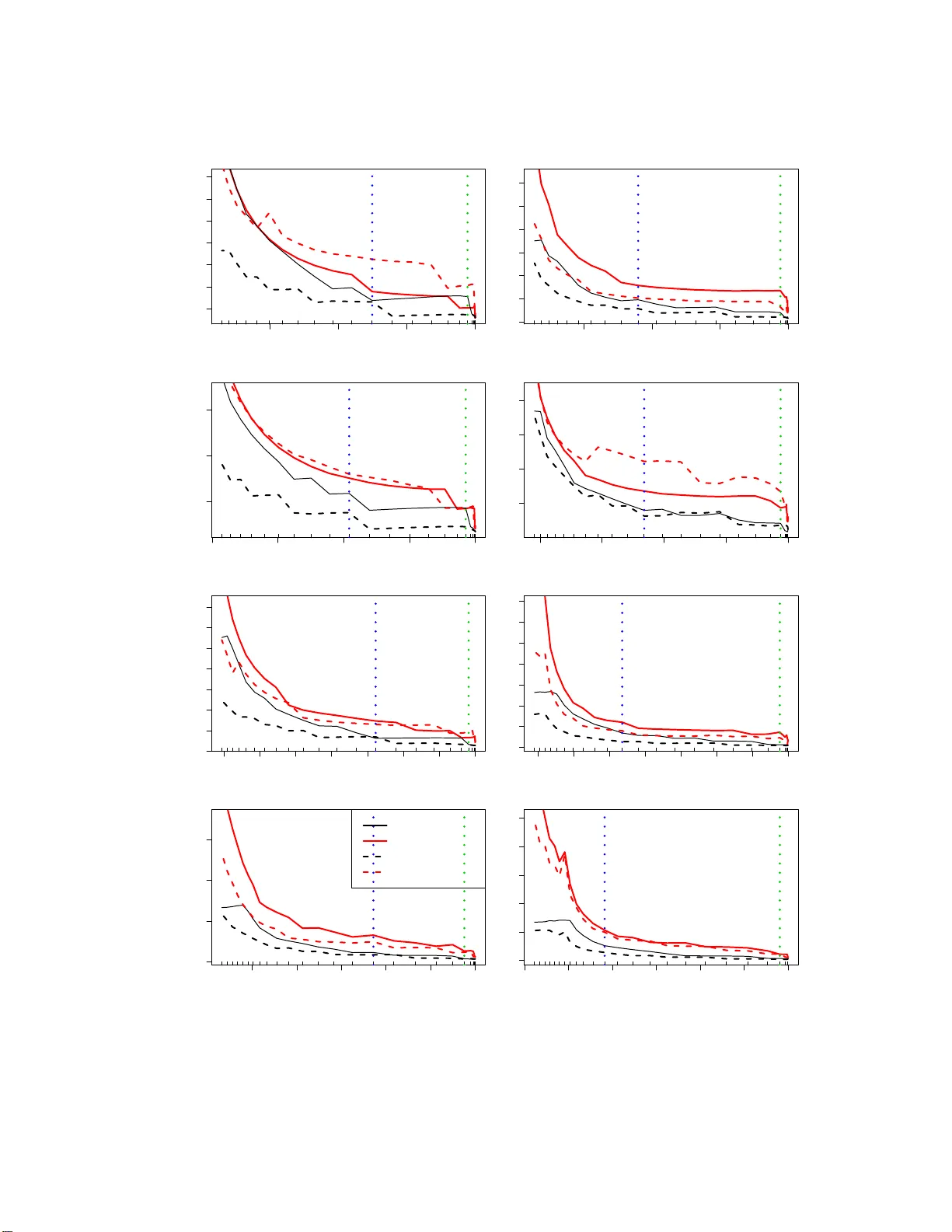
The Graphical Lasso: New Insigh ts and Alternativ es Rah ul Mazumder ∗ T rev or Hastie † Departmen t of Statistics Stanford Univ ersit y Stanford, CA 94305. Revised Dra ft on August 1, 2012 Abstract The graphical lasso [F riedman et al., 2 007 ] is an algo rithm for learning th e structure in an undirected Gaussian graphical mo del, u sing ℓ 1 regularization to control the n umber of zeros in the precision m atrix Θ = Σ − 1 [Banerjee et al., 2008 , Y uan and Lin, 2 007]. The R pac k age g lasso [F riedman et al., 2007] is popular, fast, an d allo ws one to effici ently bu ild a path of mo dels for different v alues of t he tuning parame ter. Con vergence of glasso can be tric ky; the con verged precision matrix m ight not b e the inve rse of t h e estimated cov ariance, and o ccasionally it fails to conv erge with w arm starts. In this pap er w e explain th is b ehavior, and prop ose new algorithms that app ear to outp erform glasso . By studying the “normal equations” w e s ee that, glasso is s olving the dual o f the g raphi- cal lasso p enalized likel iho o d, by bloc k co ordinate ascent; a result which ca n also b e found in Banerjee et al. [2008]. In this dual, th e target of estima tion is Σ , th e co v ariance matrix, rather than the precisi on matrix Θ . W e propose simil ar primal algorithms p-glasso and dp-glasso , that also operate by block-coordinate descent, where Θ is the optimization target. W e study all of these algorithms, and in particular different approaches to solving their co ordinate sub-problems. W e conclude that dp-glasso is sup erior from several p oints of view. 1 In tro duction Consider a data matrix X n × p , a sample of n realizations from a p - dimensional Ga ussian distr ibution with zero mean and p ositive definite c ov a r iance matrix Σ . The task is to estimate the unknown Σ based on the n samples — a c hallenging problem esp ecially when n ≪ p , when the o rdinary maximum likelihoo d estimate do es not exis t. E ven if it do es exist (for p ≤ n ), the MLE is often p o orly behaved, and regular iz ation is called for. The Graphica l Lass o [F riedman et a l., 2 007] is a r egulariza tion framework for e stimating th e cov ariance matrix Σ , under the assumption that its inv erse Θ = Σ − 1 is sparse [Banerjee et al., 200 8, Y uan and Lin, 200 7, Meinshausen and B ¨ uhlmann, 2006]. Θ is called the precision matrix; if an element θ j k = 0, this implies that the cor resp onding v ariable s X j and X k are conditionally independent, giv en the rest. O ur algorithms focus either on the res tr icted version of Θ o r its inv erse W = Θ − 1 . The graphica l lasso problem minimizes a ℓ 1 -regular ized neg ative log-likeliho o d: minimize Θ ≻ 0 f ( Θ ) := − log det( Θ ) + tr( SΘ ) + λ k Θ k 1 . (1) Here S is the s ample cov aria nce ma trix, k Θ k 1 denotes the sum of the absolute v a lues of Θ , and λ is a tuning para meter controlling the amount of ℓ 1 shrink a ge. This is a semidefinite progr amming problem (SDP) in the v aria ble Θ [Bo yd and V andenber ghe, 2004]. In this paper we revis it the glasso algorithm prop osed by F riedman et al. [2007] for solving (1); we analyze its pro p er ties, expo se problems and issues, a nd prop ose alternative algo rithms mor e suitable for the t ask . ∗ email: rah ulm@stanford.edu † email: hast ie@stanford.edu 1 Some o f the results and conclusio ns of this paper can be found in Banerjee et al. [2008], b oth explicitly and implicitly . W e re- derive some o f the results and derive new r esults, insights and algorithms, using a unified and more elemen tary fra mework. Notation W e denote the entries of a matrix A n × n by a ij . k A k 1 denotes the sum of its absolute v alues, k A k ∞ the maximu m absolute v alue of its entries, k A k F is its F rob enius norm, and a bs( A ) is the matrix with elements | a ij | . F o r a vector u ∈ ℜ q , k u k 1 denotes the ℓ 1 norm, and so o n. F ro m now on, unless otherwise sp ecified, w e will as sume that λ > 0. 2 Review of the glasso algorithm. W e use the fr ame-work o f “ normal equations” as in Hastie et al. [2009], F riedman et al. [2007]. Using sub-gradient notation, we can write the optimality conditions (ak a “normal equations” ) for a s olution to (1) a s − Θ − 1 + S + λ Γ = 0 , (2) where Γ is a ma trix of comp onent-wise signs of Θ : γ j k = sign( θ j k ) if θ j k 6 = 0 γ j k ∈ [ − 1 , 1] if θ j k = 0 (3) (w e u se the no tation γ j k ∈ Sign( θ j k )). Since the glo bal stationary conditions of (2) requir e θ j j to be po sitive, this implies that w ii = s ii + λ, i = 1 , . . . , p, (4) where W = Θ − 1 . glasso uses a blo ck-co ordinate metho d for solv ing ( 2). Co nsider a partitioning of Θ and Γ : Θ =  Θ 11 θ 12 θ 21 θ 22  , Γ =  Γ 11 γ 12 γ 21 γ 22  (5) where Θ 11 is ( p − 1) × ( p − 1), θ 12 is ( p − 1) × 1 a nd θ 22 is s c alar. W and S are pa rtitioned the same wa y . Using prop er ties o f in verses of block-partitioned ma trices, obser ve that W = Θ − 1 can be written in tw o equiv alent forms:  W 11 w 12 w 21 w 22  =   ( Θ 11 − θ 12 θ 21 θ 22 ) − 1 − W 11 θ 12 θ 22 · 1 θ 22 − θ 21 W 11 θ 12 θ 2 22   (6) =    Θ − 1 11 + Θ − 1 11 θ 12 θ 21 Θ − 1 11 ( θ 22 − θ 21 Θ − 1 11 θ 12 ) − Θ − 1 11 θ 12 θ 22 − θ 21 Θ − 1 11 θ 12 · 1 ( θ 22 − θ 21 Θ − 1 11 θ 12 )    . (7) glasso solves for a row/column of (2) at a time, holding the rest fixed. Consider ing the p th column of (2), we get − w 12 + s 12 + λ γ 12 = 0 . (8) Reading off w 12 from (6) we have w 12 = − W 11 θ 12 /θ 22 (9) and plugging into (8), we have: W 11 θ 12 θ 22 + s 12 + λ γ 12 = 0 . (10) glasso op erates o n the abov e gradient equa tion, as describ ed b elow. 2 As a v a riation consider rea ding off w 12 from (7): Θ − 1 11 θ 12 ( θ 22 − θ 21 Θ − 1 11 θ 12 ) + s 12 + λ γ 12 = 0 . (11) The ab ov e simplifies to Θ − 1 11 θ 12 w 22 + s 12 + λ γ 12 = 0 , (12) where w 22 = 1 / ( θ 22 − θ 21 Θ − 1 11 θ 12 ) is fixed (b y the globa l stationa ry conditions (4)). W e will see that these tw o apparently simila r estimating equations (10) a nd (12) lead to very different a lg orithms. The glasso alg o rithm solves (10) for β = θ 12 /θ 22 , that is W 11 β + s 12 + λ γ 12 = 0 , (13) where γ 12 ∈ Sign( β ), since θ 22 > 0. (13) is the stationarity equation for the following ℓ 1 regular iz ed quadratic pro g ram: minimize β ∈ℜ p − 1  1 2 β ′ W 11 β + β ′ s 12 + λ k β k 1  , (14) where W 11 ≻ 0 is assumed to be fixed. This is analogo us to a la sso regress io n problem of the las t v ar iable on the rest, ex c ept the cross -pro duct matr ix S 11 is r eplaced by its current estimate W 11 . This problem itself can b e solved efficien tly using element wise c o ordinate des cent, exploiting the sparsity in β . F rom ˆ β , it is eas y to o btain ˆ w 12 from (9). Using the lo wer-right element of (6), ˆ θ 22 is obtained by 1 ˆ θ 22 = w 22 − ˆ β ′ ˆ w 12 . (15) Finally , ˆ θ 12 can now be recov ered from ˆ β and ˆ θ 22 . Notice, how ever, that having solved for β and upda ted w 12 , glasso ca n mov e onto the next blo ck; disentangling θ 12 and θ 22 can b e done at the end, when the algorithm over all blo cks has con verged. The gla sso algo rithm is outlined in Algorithm 1. W e s how in Lemma 3 in Section 8 tha t the successive up dates in gla sso keep W positive definite. Algorithm 1 glasso alg orithm [F r iedman et al., 2 007] 1. Initialize W = S + λ I . 2. Cycle around the co lumns rep eatedly , per forming the following steps till conv erge nc e : (a) Rearrang e the ro ws/co lumns so that the target column is last (implicitly). (b) Solve the la sso problem (14), using as w arm starts the solution from the previous round for this column. (c) Up date the row/column (off-diagona l) of the cov ariance using ˆ w 12 (9). (d) Sav e ˆ β for this column in the ma trix B . 3. Finally , for every row/column, compute t he diagonal en tries ˆ θ j j using (15), and con vert the B matrix to Θ . Figure 1 (left panel, black curve) plots the ob jective f ( Θ ( k ) ) for the sequence o f solutions pr o duced by glasso on an example. Surprisingly , the curve is not monotone decr easing, as confirmed b y the middle plot. If glasso were solving (1) b y blo ck coor dinate-descent, w e would not anticipate this behavior. A closer lo ok at steps (9) and (10) of the glasso algo rithm leads to the following observ ations: (a) W e wish to so lve (8) for θ 12 . Howev er θ 12 is e ntangled in W 11 , whic h is (incorrectly) treated as a constant. (b) After up dating θ 12 , we see from (7) tha t the entire (w ork ing ) cov a riance matrix W changes. glasso how ever up dates only w 12 and w 21 . 3 100 200 300 400 500 −71.0 −70.5 −70.0 Iteration Index Criterion Primal Objective Dual Objective 100 200 300 400 500 −0.06 −0.02 0.02 0.04 0.06 Iteration Index Primal Differences 0 100 200 300 400 500 −0.010 0.000 0.010 0.020 Iteration Index Dual Differences Figure 1: [ L eft p anel] The obje ctive values of the pri mal criterion (1) and the dual criterion (19) c orr e- sp onding to the c ovarianc e matrix W pr o duc e d by glasso algorithm as a function of the iter ation index (e ach c olum n/r ow up date). [M idd l e Panel] The suc c essive differ enc es of the primal obje ctive values — the zer o cr ossings indic ate no n-monotonicity. [ Right Panel] The suc c essive differ enc es in the du al ob je ctive values — ther e a r e no z er o cr ossings, indic ating that glass o pr o duc es a monotone se quenc e of dual obje ctive values. These tw o observ ations explain the non-mo notone behavior of glasso in minimizing f ( Θ ). Section 3 shows a corrected block-co ordinate descent algorithm for Θ , and Section 4 shows that the glasso algorithm is actually o ptimizing the dual of problem (1 ), with the optimiza tio n v aria ble being W . 3 A Corrected glasso blo c k co ordinate-descen t algorithm Recall that (12) is a v a r iant of (10), where the dependence of the cov ariance sub-matrix W 11 on θ 12 is explicit. With α = θ 12 w 22 (with w 22 ≥ 0 fixed), Θ 11 ≻ 0 , (12) is equiv alent to the sta tionary condition for minimize α ∈ℜ p − 1  1 2 α ′ Θ − 1 11 α + α ′ s 12 + λ k α k 1  . (16) If ˆ α is the minimizer of (1 6), then ˆ θ 12 = ˆ α /w 22 . T o complete the o ptimization for the entire row/column we need to up da te θ 22 . This follows s imply from (7) ˆ θ 22 = 1 w 22 + ˆ θ 21 Θ − 1 11 ˆ θ 12 , (17) with w 22 = s 22 + λ . T o solv e (16) we need Θ − 1 11 for each blo ck up date. W e a chiev e this by maintaining W = Θ − 1 as the iterations pr o ceed. Then for each block • we obtain Θ − 1 11 from Θ − 1 11 = W 11 − w 12 w 21 /w 22 ; (18) • once θ 12 is updated, the entir e working cov ar iance matrix W is up dated (in particula r the po rtions W 11 and w 12 ), via the identities in (7), using the kno wn Θ − 1 11 . Both these steps are simple r ank-one up dates with a to tal cost of O ( p 2 ) op eratio ns . W e r efer to this as the pr imal graphica l la sso or p-glasso , which we prese nt in Algorithm 2. The p-glasso algorithm requires slightly more work tha n glasso , since an a dditional O ( p 2 ) op erations have to b e p er formed b efore and after each block update. In re tur n we ha ve that after every r ow/column up date, Θ a nd W are p ositive definite (for λ > 0) and ΘW = I p . 4 Algorithm 2 p-glasso Alg o rithm 1. Initialize W = dia g( S ) + λ I , and Θ = W − 1 . 2. Cycle around the co lumns rep eatedly , per forming the following steps till conv erge nc e : (a) Rearrang e the ro ws/co lumns so that the target column is last (implicitly). (b) Compute Θ − 1 11 using (18). (c) So lve (16) for α , using a s warm s ta rts the solution from the previo us round of row/column upda tes. Up date ˆ θ 12 = ˆ α /w 22 , and ˆ θ 22 using (17). (d) Upda te Θ a nd W us ing ( 7), ensuring that Θ W = I p . 3. Output the solutio n Θ ( precis ion) and its exact in verse W (cov arianc e ). 4 What is g lasso actually solving? Building up on the framework developed in Section 2, we now pr o ceed to e s tablish that gla sso solves the co nv ex dual of problem (1 ), b y blo ck co or dinate ascent. W e reach this conclusion via elementary arguments, closely aligned with the framework w e develop in Section 2. The approach we pr esent here is intended for an a udience without m uch of a f amilia r ity with conv ex dualit y the- ory Boyd a nd V andenberghe [200 4]. Figure 1 illustrates tha t glasso is an ascent algorithm on the dual of the pr oblem 1. The red curve in the left plot shows the dual ob jective rising monotonely , and the righ tmost plot shows that the incr e men ts a re indeed positive. There is an added twist though: in solving the blo ck-co ordina te upda te, glasso s olves instead the dua l of that subproblem. 4.1 Dual of the ℓ 1 regularized log-likel iho o d W e prese nt b elow the following lemma, the conclusion of which also a pp ea rs in Banerjee et al. [2008], but we use the framework develop ed in Section 2. Lemma 1. Consider t he primal pr oblem (1) and its stationarity c onditions (2). These ar e e quivalent to the stationarity c onditions for the b ox-c onstr aine d SDP maximize ˜ Γ : k ˜ Γ k ∞ ≤ λ g ( ˜ Γ ) := lo g det ( S + ˜ Γ ) + p (19) under the tr ansformation S + ˜ Γ = Θ − 1 . Pr o of. The (sub)g r adient conditio ns (2 ) can b e rewr itten as: − ( S + λ Γ ) − 1 + Θ = 0 (20) where Γ = sg n( Θ ). W e wr ite ˜ Γ = λ Γ and observe t hat k ˜ Γ k ∞ ≤ λ . Deno te by abs( Θ ) the matrix with element-wise a bsolute v a lue s . Hence if ( Θ , Γ ) satisfy (20), the substitut ions ˜ Γ = λ Γ ; P = abs( Θ ) (21) satisfy the following set of equations: − ( S + ˜ Γ ) − 1 + P ∗ sgn( ˜ Γ ) = 0 P ∗ (abs( ˜ Γ ) − λ 1 p 1 ′ p ) = 0 k ˜ Γ k ∞ ≤ λ. (22) In the above, P is a sy mmetric p × p matrix with non-neg ative entries, 1 p 1 ′ p denotes a p × p matrix of ones, a nd the oper ator ‘ ∗ ’ denotes elemen t-wise pro duct. W e obser ve that (22) are the K KT optimality 5 conditions for the b ox-constrained SDP (19). Similarly , the transforma tions Θ = P ∗ sg n( ˜ Γ ) a nd Γ = ˜ Γ /λ show that conditions (22) imply condition (20). Bas ed o n (2 0) the optimal solutions of the t wo problems (1) and (19) ar e related by S + ˜ Γ = Θ − 1 . Notice that for the dua l, the optimization v a riable is ˜ Γ , with S + ˜ Γ = Θ − 1 = W . In other w ords, the dual pro blem solves for W rather than Θ , a fact that is sugg ested by the glass o algorithm. Remark 1. The e quivalenc e of the solutions to pr oblems (19) and (1) as describ e d ab ove c an also b e derive d via c onvex duality the ory [Boyd a nd V andenb er ghe, 2004], whic h shows that (19) is a dual function of the ℓ 1 r e gularize d ne gative lo g-likeliho o d (1). Str ong duality holds, henc e the optimal solutions of the two pr oblems c oincide Banerje e et al. [2008]. W e now consider s olving (22) for the last blo ck ˜ γ 12 (excluding diago nal), holding the rest o f ˜ Γ fixed. The cor resp onding equations are − θ 12 + p 12 ∗ sgn( ˜ γ 12 ) = 0 p 12 ∗ (abs( ˜ γ 12 ) − λ 1 p − 1 ) = 0 k ˜ γ 12 k ∞ ≤ λ. (23) The o nly non-trivial translation is the θ 12 in the first equa tion. W e must express this in terms of the optimization v a riable ˜ γ 12 . Since s 12 + ˜ γ 12 = w 12 , us ing the iden tities in (6), we have W − 1 11 ( s 12 + ˜ γ 12 ) = − θ 12 /θ 22 . Since θ 22 > 0, we can redefine ˜ p 12 = p 12 /θ 22 , to get W − 1 11 ( s 12 + ˜ γ 12 ) + ˜ p 12 ∗ sgn( ˜ γ 12 ) = 0 ˜ p 12 ∗ (abs( ˜ γ 12 ) − λ 1 p − 1 ) = 0 k ˜ γ 12 k ∞ ≤ λ. (24) The following lemma shows that a block update of glasso so lves (24) (and hence (23)), a block of s tationary conditions for the dual of the g r aphical lass o problem. Curiously , glasso do es this no t directly , but by so lving the dual of the QP corresp onding to this blo ck of equations. Lemma 2. Assu me W 11 ≻ 0 . The statio narity e quations W 11 ˆ β + s 12 + λ ˆ γ 12 = 0 , (25) wher e ˆ γ 12 ∈ Sign ( ˆ β ) , c orr esp ond to the solution of t he ℓ 1 -r e gularize d QP: minimize β ∈ℜ p − 1 1 2 β ′ W 11 β + β ′ s 12 + λ k β k 1 . (26) Solving (26) is e quivalent to solving the following b ox-c onstr aine d QP: minimize γ ∈ℜ p − 1 1 2 ( s 12 + γ ) ′ W − 1 11 ( s 12 + γ ) sub ject to k γ k ∞ ≤ λ, (27) with stationarity c onditions given by (24), wher e the ˆ β and ˜ γ 12 ar e r elate d by ˆ β = − W − 1 11 ( s 12 + ˜ γ 12 ) . (28) Pr o of. (25) is the K KT optimality co ndition for the ℓ 1 regular iz ed Q P (26). W e rewrite (2 5) as ˆ β + W − 1 11 ( s 12 + λ ˆ γ 12 ) = 0 . (29) Observe that ˆ β i = sg n( ˆ β i ) | β i | ∀ i and k ˆ γ 12 k ∞ ≤ 1. Suppose ˆ β , ˆ γ 12 satisfy (29), then the substitutions ˜ γ 12 = λ ˆ γ 12 , ˜ p 12 = abs( ˆ β ) (30) in (29) satisfy the stationarity conditions (24). It turns out that (24) is equiv alent to the KK T optimality co nditio ns of the box-constraine d QP (27). Similar ly , w e no te that if ˜ γ 12 , ˜ p 12 satisfy (24), then the substitution ˆ γ 12 = ˜ γ 12 /λ ; ˆ β = ˜ p 12 ∗ sgn( ˜ γ 12 ) satisfies (29). Hence the ˆ β and ˜ γ 12 are related by (28). 6 Remark 2. The ab ove r esult c an also b e derive d via c onvex duality the ory[Boyd and V andenb er ghe, 2004], wher e (27) is actual ly the L agr ange dual of the ℓ 1 r e gularize d QP (26), with (28) denot- ing the primal-dual r elationship. [ Banerje e et al., 2008, Se ction 3.3] interpr et (27) as an ℓ 1 p e- nalize d r e gr ession pr oblem (u s ing c onvex duality the ory) and explor e c onne ctions with t he set up of Mei nshausen and B¨ uhlmann [20 06 ]. Note that the QP (27) is a (partial) optimizatio n ov er the v ariable w 12 only (since s 12 is fix e d); the s ub- matrix W 11 remains fixed in the QP . E x actly one row/column o f W changes when the blo ck- co ordinate alg orithm of glasso mov es to a new row/column, unlik e an explicit full matr ix update in W 11 , which is required if θ 12 is up dated. This ag a in emphasizes that glasso is o pe r ating on the cov ariance matrix instead of Θ . W e thus arrive at the f ollowing conclusion: Theorem 1. glasso p erforms blo ck-c o or dinate asc ent on the b ox-c onstr aine d SDP (19), t he L agr ange dual of the primal pr oblem (1). Each of the blo ck steps ar e themselves b ox-c onstr aine d QPs, which glasso optimizes via their L agr ange duals. In our anno tation p erhaps glasso should be called dd -glasso , since it p erforms dual blo ck upda tes for the dual of the graphical lasso problem. Banerjee et a l. [2008], the pap er that inspired the original glasso ar ticle [F riedman et a l., 2 007], also op erates on the dua l. They how ever solve the blo ck-updates dire ctly (whic h a re b ox co nstrained QPs) using interior-p oint metho ds. 5 A New Algorithm — d p-glasso In Section 3, w e desc r ib ed p-glasso , a pr imal co o rdinate-descent metho d. F or e very row/column we need to solv e a lasso problem (16), whic h o p erates on a quadratic for m corresp onding to the square matrix Θ − 1 11 . There are tw o problems with this a pproach: • the matrix Θ − 1 11 needs to b e co nstructed at every row/column up date with co mplexity O ( p 2 ); • Θ − 1 11 is dense. W e now show ho w a simple mo dificatio n of the ℓ 1 -regular ized QP leads to a b ox-constrained Q P with attractive computational prop erties. The KKT optimality conditions for (16), following (12), can b e written a s: Θ − 1 11 α + s 12 + λ sgn( α ) = 0 . (31) Along the same lines of the deriv ations used in Lemma 2 , the condition above is equiv a lent to ˜ q 12 ∗ sgn( ˜ γ ) + Θ 11 ( s 12 + ˜ γ ) = 0 ˜ q 12 ∗ (abs( ˜ γ ) − λ 1 p − 1 ) = 0 k ˜ γ k ∞ ≤ λ (32) for some vector (with non-nega tive entries) ˜ q 12 . ( 32) ar e the KKT optimality co nditions for the following b ox-constra ined QP: minimize γ ∈ℜ p − 1 1 2 ( s 12 + γ ) ′ Θ 11 ( s 12 + γ ); sub ject to k γ k ∞ ≤ λ. (33) The optimal solutions o f (33) and (31) a re related by ˆ α = − Θ 11 ( s 12 + ˜ γ ) , (34) a consequence o f (31), with ˆ α = ˆ θ 12 · w 22 and w 22 = s 22 + λ . T he dia gonal θ 22 of the pr ecision matrix is up dated via (7 ): ˆ θ 22 = 1 − ( s 12 + ˜ γ ) ′ ˆ θ 12 w 22 (35) 7 Algorithm 3 dp-glasso a lgorithm 1. Initialize Θ = diag ( S + λ I ) − 1 . 2. Cycle around the co lumns rep eatedly , per forming the following steps till conv erge nc e : (a) Rearrang e the ro ws/co lumns so that the target column is last (implicitly). (b) Solve (33 ) for ˜ γ and up date ˆ θ 12 = − Θ 11 ( s 12 + ˜ γ ) /w 22 (c) So lve for θ 22 using (35). (d) Upda te the w o rking cov ariance w 12 = s 12 + ˜ γ . By strong duality , the box-constrained QP (33) with its optimality co nditio ns (32) is eq uiv alent to the la s so pr oblem (16). Now b oth the pr o blems listed at the b eg inning of the sec tio n are removed. The problem matrix Θ 11 is spar se, and no O ( p 2 ) up dating is req uired after each blo ck. The solutions returned a t step 2(b) for ˆ θ 12 need not be exactly sparse, even though it purports to pr o duce the solution to the primal blo ck problem (1 6), which is spa rse. One needs to use a tight conv ergence criterio n when so lving (33). In addition, one ca n threshold those elements of ˆ θ 12 for which ˜ γ is awa y fr om the b ox b ounda ry , since those v a lues are known to be zero. Note that dp-glasso does to the primal formulation (1) what glasso do es to the dual. dp- glasso op erates o n the precision matrix, whereas glasso op er ates on the cov ariance matrix. 6 Computational Costs in Solving the Blo c k QPs The ℓ 1 regular iz ed Q Ps app earing in (14) a nd (16) are o f the g eneric form minimize u ∈ℜ q 1 2 u ′ Au + a ′ u + λ k u k 1 , (36) for A ≻ 0 . In this pap er , w e cho ose to use cyc lical co o rdinate desce nt for solving (36), as it is used in the glasso algor ithm implementation of F rie dma n et al. [200 7]. Moreover, cyclica l co o rdinate descent metho ds per fo rm well with go o d warm-starts. These a re av ailable for bo th (14) and (16), since they b o th maintain working copies of the pre c ision matrix, upda ted after ev ery row/column upda te. Ther e are o ther efficient wa ys for so lving (36), c a pable of sca ling to larg e pr oblems — for example first-order pr oximal metho ds [Beck and T eb oulle, 2009, Nesterov , 2007], but w e do not pursue them in this pap er. The box-constra ined Q Ps app earing in (27) a nd (33) are of the generic form: minimize v ∈ℜ q 1 2 ( v + b ) ′ ˜ A ( v + b ) sub ject to k v k ∞ ≤ λ (37) for some ˜ A ≻ 0 . As in the ca s e ab ov e, w e will use cyclica l co ordinate-des c ent for optimizing (37 ). In genera l it is more efficient to solve (36) than (37) for larger v alues of λ . This is beca use a lar ge v alue of λ in (36 ) re sults in spar se solutions ˆ u ; the co ordinate des c e n t a lgorithm ca n ea sily detect when a zero stays zero, and no further work gets done for that co ordinate on that pas s . If the solution to (36) ha s κ non-zer os, then on av erage κ co ordina tes nee d to be up dated. This leads to a cost of O ( q κ ), for o ne full sweep across all the q co ordinates. On the other hand, a lar ge λ for (37) co rresp onds to a weakly-regular iz ed solutio n. Cyclical co ordinate pr o cedures for this task ar e not as effective. E very co o rdinate up date o f v results in upda ting the gradien t, which requires adding a sca lar multiple of a column of ˜ A . If ˜ A is dense, this leads to a cost of O ( q ), and for o ne full cycle acros s all the co or dinates this costs O ( q 2 ), rather than the O ( q κ ) f or (3 6). 8 How ever, our exp erimental r esults show that dp-glasso is more efficient than glasso , so there are some other factors in play . When ˜ A is sparse, there are computationa l savings. If ˜ A has κq non-zeros , the cost per c o lumn reduces on average to O ( κq ) from O ( q 2 ). F or the formulation (33) ˜ A is Θ 11 , which is sparse for large λ . Hence f or la rge λ , glasso and dp-glasso ha ve similar cos ts. F or smaller v alues of λ , the b ox-constrained QP (37 ) is particularly attra ctive. Most o f the co ordinates in the optimal solution ˆ v will pile up at the bo undary p o ints { − λ, λ } , which means that the co o rdinates need not be up dated frequently . F or problem (33) this num b er is a lso κ , the nu mber of no n-zero coefficients in the corresp o nding c o lumn o f the precisio n matrix. If κ of the co ordinates pile up at the b oundary , then one full sweep of cyclical co o rdinate descent acro ss all the co o r dinates will require up da ting gradients co rresp onding to the r emaining q − κ co o rdinates. Using s imilar calculations as befor e, this will cost O ( q ( q − κ )) op era tio ns p er full cycle (since for small λ , ˜ A will be dense ). F or the ℓ 1 regular iz ed problem (36), no such s aving is a chiev ed, and the cost is O ( q 2 ) per cycle. Note that to solve problem (1), we nee d to so lve a QP of a par ticular type (36) o r (37) for a certain n um b er of outer cycles (ie full s weeps acr oss r ows/columns). F or every row/column update, the asso c iated QP requires v ary ing n umber of iter ations to conv erge. It is hard to characterize all these factors and come up with precise estimates of co nv ergence r ates of the ov era ll algo rithm. How ever, we have observed that with warm-star ts, on a r elatively dense gr id of λ s, the complexities given ab ov e ar e pretty m uch accurate for dp-glasso (with warmstarts) sp ecially when o ne is interested in so lutions with small / mo dera te accura cy . Our ex p er imental results in Section 9.1 and App endix Section B supp ort our o bserv ation. W e will now ha ve a more critical lo o k at the up dates of the glasso alg orithm and study their prop erties. 7 glasso : P ositiv e defin iteness, Sparsit y and Exact In v ersion As noted ea rlier, glasso oper ates o n W — it do es not explicitly compute the in verse W − 1 . It do es how ever keep track of the estimates for θ 12 after every row/column up date. The copy of Θ retained by gla sso along the row/column up dates is not the exact inv erse of the optimization v ar iable W . Figure 2 illustrates this by plotting the square d- norm k ( Θ − W − 1 ) k 2 F as a function o f the iteration index. Only upo n (asymptotic) c o nv ergence, will Θ be equa l to W − 1 . This can hav e impor tant consequences. 0 100 200 300 0 2 4 6 8 Iteration Inde x Error in Inv erse 0 100 200 300 −6 −2 0 2 Iteration Inde x Minimal Eigen V alue Figure 2: Fi gur e il l ustr ating some ne gative pr op erties of glasso usi ng a typic al numeric al example. [L ef t Panel] The pr e cision matrix pr o duc e d after every r ow/c olumn up date ne e d not b e the exact inverse of the working c ovarianc e matrix — the squar e d F r ob enius norm of the err or i s b eing plotte d acr oss iter ations. [Right Panel] The estimate d pr e cision matrix Θ pr o duc e d by glasso ne e d not b e p ositive definite along iter ations; plot shows mini mal eigen-value. 9 In many r eal-life problems one only ne e ds an approximate so lution to (1): • for computational re asons it might b e impr actical to obtain a solution o f high accurac y; • from a statistical viewp o int it might b e sufficient to obtain a n approximate solution fo r Θ that is b oth sparse and po sitive definite It turns o ut that the glasso a lgorithm is not s uited to this pu rp os e. Since the glasso is a blo ck co o rdinate pro cedure on the cov a riance matrix, it maintains a positive definite cov ariance matrix at ev ery row/column up date. Howev er, since the estimated precision matrix is not the exac t inv erse of W , it need not be p ositive definite. Although it is rela tively straightforw ar d to maintain an exact in verse of W along the row/column updates (via simple rank -one updates as befo re), this in verse W − 1 need not b e s parse. Arbitrary thresho lding rules may b e used to set some o f the entries to zero , but that might des tr oy the p ositive-definiteness of the matrix. Since a pr inc ipa l motiv a tion of solving (1) is to o btain a sparse precision ma trix (which is als o p ositive definite), retur ning a dense W − 1 to (1) is not desir able. Figures 2 illustra tes the abov e observ ations on a t ypical exa mple. The dp-glasso algor ithm oper ates on the prima l (1). Instea d of optimizing the ℓ 1 regular iz ed QP (1 6), which r equires co mputing Θ − 1 11 , dp-glasso o ptimizes (33). After every row/column up date the pr ecision matrix Θ is p ositive definite. The working cov ar iance matrix maintained by dp-glasso via w 12 := s 12 + ˆ γ need no t b e the exac t inv erse of Θ . Exa ct cov aria nce matrix estimates, if required, can b e obtained by tracking Θ − 1 via simple ra nk-one upda tes , as descr ibed ea rlier. Unlik e glasso , dp-glasso (a nd p-glasso ) re tur n a spar se and p os itive definite pr ecision ma trix even if the ro w/column iterations ar e ter minated prematurely . 8 W arm Starts and P ath-seeking Strategies Since we seldom know in a dv ance a go o d v alue of λ , we often co mpute a sequence of s olutions to (1 ) for a (t ypically ) decr easing seq uence of v alues λ 1 > λ 2 > . . . > λ K . W arm-sta rt or contin uation metho ds use the solution a t λ i as an initial gues s for the solution at λ i +1 , and often yield great efficiency . It turns o ut that for algorithms like glasso which op era te on the dual problem, not all warm-starts necessarily lead t o a co nvergen t algorithm. W e addr e ss this asp ect in detail in this s ection. The following lemma states the conditions under whic h the row/column up dates of the glasso algorithm will ma int ain p ositive definiteness of the cov aria nce matrix W . Lemma 3. Supp ose Z is use d as a warm-start for the glasso algorithm. If Z ≻ 0 and k Z − S k ∞ ≤ λ , then every r ow/c olumn u p date of glasso maintains p ositive definiteness of the working c ovarianc e matrix W . Pr o of. Recall that the glasso solves the dual (19). Assume Z is partitioned as in (5), and t he p th row/column is being up dated. Since Z ≻ 0 , we have b oth Z 11 ≻ 0 and  z 22 − z 21 ( Z 11 ) − 1 z 12  > 0 . (38) Since Z 11 remains fixed, it suffices to show that after the row/column up da te, the expressio n ( ˆ w 22 − ˆ w 21 ( Z 11 ) − 1 ˆ w 12 ) remains p ositive. Recall that, v ia standar d optimality conditions we hav e ˆ w 22 = s 22 + λ , which mak es ˆ w 22 ≥ z 22 (since by assumption, | z 22 − s 22 | ≤ λ a nd z 22 > 0). F urthermor e , ˆ w 21 = s 21 + ˆ γ , where ˆ γ is the optimal solution to the co rresp onding b ox-QP (27). Since the sta rting solution z 21 satisfies the b ox-constraint (27) i.e. k z 21 − s 21 k ∞ ≤ λ , the optimal solution of the Q P (27) improv es the ob jective: ˆ w 21 ( Z 11 ) − 1 ˆ w 12 ≤ z 21 ( Z 11 ) − 1 z 12 Combining the a b ove a long with the fact that ˆ w 22 ≥ z 22 we see ˆ w 22 − ˆ w 21 ( Z 11 ) − 1 ˆ w 12 > 0 , (39) which implies that the new co v a riance estimate c W ≻ 0 . 10 Remark 3. If the c ondition k Z − S k ∞ ≤ λ app e aring in L emma 3 is vio late d, then the r ow/c olumn up date of glasso ne e d not maintain PD of the c ovarianc e matrix W . W e hav e encountered ma ny counter-examples that show this to be true, see the discussion b elow. The R pack age implementation of gla sso allows the user to spe c ify a warm-start as a tuple ( Θ 0 , W 0 ). This option is t y pic a lly used in the cons tr uction of a path algo rithm. If ( b Θ λ , c W λ ) is provided as a warm-start for λ ′ < λ , then the glasso algorithm is not guaranteed to conv erge. It is easy to find numerical examples by c ho osing the gap λ − λ ′ to b e larg e enough. Among the v ar ious examples w e encount ered, we briefly describ e one here. Details of the exper iment /da ta and other exa mples can b e found in the online Appendix A.1. W e generated a data-matrix X n × p , with n = 2 , p = 5 with iid standard Ga ussian entries. S is the sample c ov a riance matr ix. W e solved problem (1) using glasso for λ = 0 . 9 × max i 6 = j | s ij | . W e to ok the es timated co v a riance a nd precision m atr ic e s: c W λ and b Θ λ as a w arm-star t for the glasso algorithm with λ ′ = λ × 0 . 01 . The glasso algor ithm failed to con verge with this w arm-star t. W e note that k c W λ − S k ∞ = 0 . 0 402  λ ′ (hence violating the sufficient condition in Lemma 4) and a fter up dating the fir st r ow/column via the glasso algo rithm we obser ved that “cov ariance ma trix” W ha s nega tive eigen- v alues — leading to a non-co nv ergent algorithm. The ab ov e pheno meno n is not surpr ising and easy to expla in and generalize. Since c W λ solves the dual (19), it is necess a rily of the form c W λ = S + ˜ Γ , for k ˜ Γ k ∞ ≤ λ . In the ligh t of Lemma 3 and also Remark 3, the w arm- start needs to b e dua l- feasible in order to guarantee that the iter ates c W remain P D and hence for the sub-problems to be well defined conv ex progra ms. Clearly c W λ do es not sa tis fy the b ox-constraint k c W λ − S k ∞ ≤ λ ′ , for λ ′ < λ . How ever, in practice the glasso a lgorithm is usually seen to converge (nu merica lly) when λ ′ is quite close to λ . The following lemma es tablishes that an y PD ma trix can b e taken as a warm-start for p-glasso or dp-glasso to e ns ure a conv ergent algor ithm. Lemma 4. Supp ose Φ ≻ 0 is a use d as a warm-start for the p-glasso (or dp-glasso ) algorithm. Then every r ow/c olumn up date of p-glasso (or dp-glasso ) maintains p ositive definiteness of the working pr e cision matrix Θ . Pr o of. Consider up dating the p th row/column of the precisio n matrix . The condition Φ ≻ 0 is equiv ale nt to b oth Φ 11 ≻ 0 and  φ 22 − Φ 21 ( Φ 11 ) − 1 Φ 12  > 0 . Note that the blo ck Φ 11 remains fixed; only the p th row/column o f Θ changes. φ 21 gets updated t o ˆ θ 21 , as do es ˆ θ 12 . F r om (7) the up dated diagonal en try ˆ θ 22 satisfies: ˆ θ 22 − ˆ θ 21 ( Φ 11 ) − 1 ˆ θ 12 = 1 ( s 22 + λ ) > 0 . Thu s the up dated matrix ˆ Θ remains PD. The result for the dp-glasso algo rithm follows, since b oth the versions p-glasso and dp-glasso solve the same blo ck coo r dinate problem. Remark 4 . A simple c onse qu en c e of L emmas 3 and 4 is that the QPs arising in the pr o c ess, namely the ℓ 1 r e gularize d QPs (14), (16) and the b ox-c onstr aine d Q Ps (27) and (33) ar e al l valid c onvex pr o gr ams, sinc e al l the r esp e ctive matric es W 11 , Θ − 1 11 and W − 1 11 , Θ 11 app e aring in the quadr atic forms ar e PD. As exhibited in Lemma 4, both the algo rithms dp-glasso and p-glasso are guar anteed to conv erge from any p ositive-definite warm start. This is due to the unconstrained formulation of the primal problem (1). glasso really only requires a n initialization for W , since it constr ucts Θ on the fly . Likewise dp-glasso only requires an initializatio n for Θ . Having the other half of the tuple assists in the blo ck-updating algorithms. F or example, glasso solves a series of lasso problems, where Θ play the role as parameter s. By supplying Θ along with W , the blo ck-wise lasso problems can b e given starting v alues close to the so lutions. The same applies to dp-glasso . In neith er case do the pairs hav e to be in verses of e ach other to s e r ve this purp os e . 11 If we wish to start with inv erse pairs , and maint ain suc h a rela tio nship, we have describ ed earlier how O ( p 2 ) up dates a fter ea ch block optimizatio n ca n achieve this. One cav eat for glasso is that starting with an inv erse pa ir cos ts O ( p 3 ) op er ations, sinc e w e typically sta r t with W = S + λ I . F or dp-glasso , we typically start with a diagonal matrix, whic h is triv ial to inv ert. 9 Exp erimen tal Results & T iming Comparisons W e compar ed the per formances of algo rithms glasso and dp-glasso (bo th with and without warm- starts) on differ ent examples with v a rying ( n, p ) v alues. While most of the results ar e presented in this se c tion, some a re releg ated to the online App endix B. Section 9.1 descr ibe s some synthetic examples and Sectio n 9.2 presents c omparisons on a rea l-life micro-ar ray data - set. 9.1 Syn thetic Exp eriments In this section we present exa mples generated fro m tw o different cov a r iance mo dels — as characterized by the cov a r iance matrix Σ or eq uiv alently the precision ma trix Θ . W e crea te a data matrix X n × p by drawing n independent samples from a p dimensional normal distribution MVN( 0 , Σ ). The sample cov ariance matrix is taken a s t he input S to pr o blem (1). The tw o co v ar iance mo dels are descr ib ed below: T yp e-1 The p opula tion concentration matrix Θ = Σ − 1 has unifor m spa rsity with a pproximately 77 % of the entries zero. W e created the cov ar ia nce matrix a s follows. W e g enerated a matrix B with iid s ta ndard Gaussian entries, symmetrized it via 1 2 ( B + B ′ ) and set appr oximately 77% of the e ntries of this ma trix to zer o, to o btain ˜ B (s ay). W e added a s calar multiple of the p dimensional identit y matrix to ˜ B to get the pre c is ion matrix Θ = ˜ B + η I p × p , with η c hosen such that the minim um eigen v alue o f Θ is one. T yp e-2 This example, taken from Y ua n and Lin [20 07], is an auto- r egress ive pro cess of o rder tw o — the precis ion matrix being tri-diagonal: θ ij =          0 . 5 , if | j − i | = 1 , i = 2 , . . . , ( p − 1); 0 . 25 , if | j − i | = 2 , i = 3 , . . . , ( p − 2); 1 , if i = j, i = 1 , . . . , p ; and 0 otherwise . F or each o f the tw o set-ups Typ e-1 and Type-2 we cons ider tw elve different c o mbinations o f ( n, p ): (a) p = 1000 , n ∈ { 150 0 , 1 000 , 500 } . (b) p = 8 00, n ∈ { 100 0 , 8 00 , 500 } . (c) p = 5 00, n ∈ { 800 , 5 0 0 , 200 } . (d) p = 2 00, n ∈ { 500 , 20 0 , 5 0 } . F or every ( n, p ) w e solv ed (1) on a grid of t wen t y λ v alues linearly spaced in the log-sca le, with λ i = 0 . 8 i × { 0 . 9 λ max } , i = 1 , . . . , 20 , where λ max = max i 6 = j | s ij | , is the o ff-diagonal en try of S with largest a bsolute v alue. λ max is the smallest v alue of λ for which the solution to (1 ) is a diagona l matrix. Since this article fo cuses on the glasso algo rithm, its pr op erties a nd alterna tives that stem from the main idea of blo ck-co ordina te optimization, we pres ent here the p er formances of the following algorithms: Dual-Cold glasso with initializa tion W = S + λ I p × p , as sugg ested in F riedman et al. [2007]. 12 Dual-W arm The path-wise version of glasso with w arm- starts, as suggested in F r iedman et al. [2007]. Althoug h this path-wise v ersion need not con verge in genera l, this w as not a pr oblem in our exp eriments, probably due to the fine- grid of λ v a lues. Primal-Cold dp-glasso with dia gonal initialization Θ = (diag( S ) + λ I ) − 1 . Primal-W arm The pa th-wise version o f dp-g lasso with w a rm-star ts. W e did not include p-glasso in the compariso ns above s ince p-glasso r e quires additional matrix rank-one up dates after every r ow/column up date, w hich ma kes it more exp ensive. None of the ab ov e listed algor ithms require matrix inv ersions (via rank one upda tes). F urthermore, dp-glasso and p-glasso are quite similar a s b oth ar e doing a blo ck coo rdinate optimization o n the dual. Hence we o nly included dp-glasso in our comparis o ns. W e used our own implemen tation of the glasso and dp-glasso algorithm in R. The en tire program is wr itten in R, except the inner block-update solvers, which are the real work-hor ses: • F or glasso we used the las so code c ro s sPro dLa sso written in F OR TRAN b y F riedma n et al. [2007]; • F or dp- glasso w e wrote our own FOR TRAN co de t o so lve the b ox QP . An R pack age implementin g dp-g lasso will be made av ailable in CRAN. In the figure and tables that follow be low, for every algorithm, at a fixed λ we rep ort the total time taken by al l the QPs — the ℓ 1 regular iz ed QP for glasso and the b ox constrained QP for dp- glasso till conv ergence All computations were do ne on a Lin ux machine with mo del sp ecs: I ntel(R) Xeon(R) CPU 51 60 @ 3.00GHz. Con v ergence Cri terion: Since dp-glasso ope rates on the the primal formulation and glasso op erates on the dual — to make the conv erg ence criter ia co mpa rable acr o ss examples we bas ed it on the relative c hange in the pr imal ob jective v alues i.e. f ( Θ ) (1) across t wo successive iterations: f ( Θ k ) − f ( Θ k − 1 ) | f ( Θ k − 1 ) | ≤ TOL , (40) where one iteratio n refers to a full sweep acro ss p rows/columns of the precis ion matrix (for dp-glasso ) and co v ar iance matr ix (for g lasso ); and TOL denotes the to lerance lev el or lev el of ac c uracy of the solution. T o compute the primal ob jective v alue for the glasso algorithm, the precision matrix is computed from c W via dir ect inversion (the time taken fo r in version and ob jective v alue co mputation is not included in the timing comparisons). Computing the ob jective function is quite exp ensive r e la tive to the computational cost of the iterations. In our exp erience con vergence cr iteria ba sed on a relative change in the precision matr ix for dp-glasso and the cov aria nce matrix fo r glasso seemed to be a practical choice for the exa mples we c o nsidered. Ho wev er, for reas ons w e describ ed ab ove, we us e d criterio n 4 0 in the exp eriments. Observ ations: Figure 4 presents the times taken b y the alg orithms to con verge to an accurac y o f TOL = 1 0 − 4 on a gr id of λ v alues. The figure shows eigh t different scena rios with p > n , corresp onding to the tw o different cov ar iance mo dels T yp e-1 (left panel) and Type- 2 (right pa ne l). It is quite evident that dp-glasso with warm- starts (Primal-W arm) outper forms all the other a lgorithms across all the different exa mples. All the algorithms conv erge quickly for lar ge v alues of λ (typically high spar sity) and b ecome slower with decreasing λ . F or larg e p a nd small λ , conv ergence is slow; how ever f or p > n , the no n-sparse end of the r e g ularizatio n path is really not that int eres ting from a s tatistical viewpo int. W arm-star ts apparently do not alwa ys help in s p eeding up the conv erg ence of glasso ; fo r exa mple see Figure 4 with ( n, p ) = (500 , 1000 ) (T yp e 1) and ( n, p ) = (50 0 , 800) (Type 2). This probably further v a lida tes the fact that warm-star ts in the ca se o f glasso need to be ca r efully desig ned, in order for them to sp e e d-up co nv ergence. Note howev er, that glasso with the warm-starts pr escrib ed is not even 13 guaranteed to conv erg e — we how ever did not co me a cross any such instance a mong the exper iment s presented in t his section. Based on the suggestio n of a re fer ee we annota ted the plots in Figure 4 with lo cations in the regular iz ation path that ar e o f interest. F o r ea ch plot, tw o vertical dotted lines are drawn which corres p o nd to the λ s at which the dista nce of the estimated precisio n ma trix b Θ λ from the p opulation precision m atr ix is minimized wrt to the k · k 1 norm (gr een) and k · k F norm (blue). The optimal λ corres p o nding to the k · k 1 metric choo ses sparser mo dels than those chosen b y k · k F ; the p erfo r mance gains achiev ed b y dp- glasso see m to b e mo re prominent for th e latter λ . T able 1 prese nts the timings for all the four algorithmic v a riants o n the t welv e different ( n, p ) combinations lis ted abov e for T y pe 1. F or every exa mple, w e rep ort the to tal time till co nv ergence on a grid of t wen t y λ v alues for tw o differen t tolerance levels: TOL ∈ { 10 − 4 , 10 − 5 } . Note that the dp-glasso returns p ositive definite and spa r se precisio n ma trices even if the algorithm is ter minated at a re la tively small/mo dera te accuracy level — this is not the cas e in glasso . The rightmost column pr esents the pr op ortion of non-zero s averaged across the en tire pa th of solutions b Θ λ , wher e b Θ λ is obtained by solving (1) to a high precision i.e. 10 − 6 , by algorithms glasso and dp-glasso and av era ging the res ults. Again w e see tha t in all the examples dp-glasso with w arm-sta rts is the clear winner among its comp etitors. F or a fixed p , the total time to tr ace out the pa th generally dec r eases with incr easing n . There is no clear winner betw een glasso with w ar m-starts and g lasso without w arm- starts. It is often s e en that dp-glasso without warm-starts co nv erges faster tha n bo th the v ariants of glasso (with and without warm-star ts). T able 2 rep orts the tim ing compa r isons fo r T yp e 2. Once again w e see that in all the examples Primal-W arm turns out to b e the c le a r winner. F or n ≤ p = 1000, we o bserve that Primal-W arm is gener ally faster for Type- 2 than Type-1 . This how ever, is rev ersed for smaller v alues of p ∈ { 80 0 , 5 00 } . P rimal-Cold is has a smaller ov erall computation time for Type-1 ov er T yp e-2. In so me cases (for example n ≤ p = 1 000), we see that Primal-W arm in Type-2 converges m uch fas ter than its comp etitor s on a relative sca le than in Type-1 — this difference is due to the v aria tions in the structure of the co v ar iance ma tr ix. 9.2 Micro-arra y Example W e c o nsider the data-set introduced in Alon et a l. [1999] a nd fur ther studied in Rothman et al. [2008], Mazumder and Hastie [2 012]. In this exp er iment, tissue samples were analyz ed using a n Affymetrix Oligonucleotide array . The data was pro c e ssed, filtered and reduced to a subset of 2000 gene expres sion v alues. The n umber of Co lon Adeno carcino ma tis s ue samples is n = 62. F o r the purp ose o f the exp eriments presented in this section, w e pr e-screened the genes to a siz e of p = 725. W e obtained this subset of g e nes using the idea of exact c ovarianc e t hr esholding in tro duced in our pap er [Mazumder and Has tie, 20 12]. W e thre s holded the sample c orrela tion matrix obtained from the 62 × 20 00 micr oarr ay data-matrix into connected compo nents with a thre shold of 0 . 003 64 1 — the gene s b elonging to the largest connected comp onent formed our pre-scr eened gene p o ol of size p = 725. This (subset) da ta-matrix of size ( n, p ) = (6 2 , 7 25) is used for our exp er iment s. The results presented below in T able 3 show timing compar isons o f the four different algorithms: Primal-W arm/Co ld and Dual-W ar m/Cold on a grid of fifteen λ v alues in the lo g-scale. Once again we see that the Prima l-W a r m outperfor ms the others in terms of sp eed a nd accuracy . Dual- W ar m per forms quite well in this example. 10 Conclusions This paper explores some of the apparen t m ysteries in the behavior of the glasso a lgorithm in tro- duced in F riedman et al. [2007]. Thes e have b een explained by leveraging th e fact that the glasso algorithm is solving the dual of the graphical la s so problem (1 ), b y blo ck coo r dinate ascent. Each blo ck update, it self the solution to a convex prog ram, is solved via its o wn dual, which is equiv alent 1 this is the largest v alue of the threshold for which the size of the largest connected comp onen t is small er than 800 14 0.4 0.6 0.8 1.0 100 200 300 400 500 600 700 0.4 0.6 0.8 1.0 0 200 400 600 800 1000 0.2 0.4 0.6 0.8 1.0 50 100 150 0.2 0.4 0.6 0.8 1.0 100 200 300 400 0.3 0.4 0.5 0.6 0.7 0.8 0.9 1.0 0 20 40 60 80 100 120 140 0.3 0.4 0.5 0.6 0.7 0.8 0.9 1.0 0 50 100 150 200 250 300 350 0.5 0.6 0.7 0.8 0.9 1.0 0 5 10 15 Primal−Cold Dual−Cold Primal−Warm Dual−W ar m 0.4 0.5 0.6 0.7 0.8 0.9 1.0 0 5 10 15 20 25 Propor tion of Zeros Propor tion of Zeros Time in Seconds Time in Seconds Time in Seconds Time in Seconds Type = 1 Type = 2 n = 50 0 /p = 1 000 n = 50 0 /p = 1 000 n = 500 / p = 800 n = 500 / p = 800 n = 200 / p = 500 n = 200 / p = 500 n = 50 /p = 20 0 n = 50 /p = 20 0 Figure 3: T he timi ngs in se c onds for the four differ ent algorithmic versions: g lasso (with and without warm- starts) and dp-glasso (with and without warm-starts) for a grid of λ values on the lo g-sc ale. [L eft Panel] Covarianc e mo del for T yp e-1, [R ight Panel] Covarianc e mo del f or T yp e-2. The horizont al axis is index e d by the pr op ortion of zer os in the solution. The vertic al dashe d lines c orr esp ond to the optimal λ values f or which the estimate d err ors k b Θ λ − Θ k 1 (gr e en) an d k b Θ λ − Θ k F (blue) ar e minimum. 15 p / n relative T ota l time (secs) to compute a path of s olutions Average % error (TOL) Dual-Cold Dual-W arm Prima l-Cold Primal-W arm Z eros in path 1000 / 500 10 − 4 3550.7 1 6592.6 3 2558.83 2005.25 80.2 10 − 5 4706.2 2 8835.5 9 3234.97 2832.15 1000 / 100 0 10 − 4 2788.3 0 3158.7 1 2206.95 1347.05 83.0 10 − 5 3597.2 1 4232.9 2 2710.34 1865.57 1000 / 150 0 10 − 4 2447.1 9 4505.0 2 1813.61 9 3 2.34 85.6 10 − 5 2764.2 3 6426.4 9 2199.53 1382.64 800 / 500 10 − 4 1216.3 0 2284.5 6 928.37 541.66 78.8 10 − 5 1776.7 2 3010.1 5 1173.76 7 9 8.93 800 / 800 10 − 4 1135.7 3 1049.1 6 788.12 438.46 80.0 10 − 5 1481.3 6 1397.2 5 986.19 614.98 800 / 1000 10 − 4 1129.0 1 1146.6 3 786.02 453.06 80.2 10 − 5 1430.7 7 1618.4 1 992.13 642.90 500 / 200 10 − 4 605.45 55 9 .14 395.1 1 191 .88 75.9 10 − 5 811.58 79 5 .43 520.9 8 282 .65 500 / 500 10 − 4 427.85 24 1 .90 252.8 3 123 .35 75.2 10 − 5 551.11 31 5 .86 319.8 9 182 .81 500 / 800 10 − 4 359.78 27 9 .67 207.2 8 111 .92 80.9 10 − 5 416.87 40 2 .61 257.0 6 157 .13 200 / 50 10 − 4 65.87 50.99 37.40 23.32 75.6 10 − 5 92.04 75.06 45.88 35.81 200 / 200 10 − 4 35.29 25.70 17.32 11.72 66.8 10 − 5 45.90 33.23 22.41 17.16 200 / 300 10 − 4 32.29 23.60 16.30 10.77 66.0 10 − 5 38.37 33.95 20.12 15.12 T able 1 : T able showing the p erformanc es of the four algorithms glasso (Dual-Warm/Cold) and dp-glasso (Primal-Warm/Cold) for the c ovarianc e mo del T yp e-1. We pr esent the tim es (in se c onds) r e quir e d to c ompute a p ath of solutions to (1) (on a g rid of twenty λ values) for differ ent ( n, p ) c ombinations and r elative e rr ors (as i n (40)). The rightmost c olumn gives the aver age d sp arsity level acr oss the g rid of λ values. dp-glasso with warm-starts is c onsistently the wi nner acr oss al l the examples. 16 p / n relative T ota l time (secs) to compute a path of s olutions Average % error (TOL) Dual-Cold Dual-W arm Prima l-Cold Primal-W arm Z eros in path 1000 / 500 10 − 4 6093.1 1 5483.0 3 3495.67 1661.93 75.6 10 − 5 7707.2 4 7923.8 0 4401.28 2358.08 1000 / 100 0 10 − 4 4773.9 8 3582.2 8 2697.38 1015.84 76.70 10 − 5 6054.2 1 4714.8 0 3444.79 1593.54 1000 / 150 0 10 − 4 4786.2 8 5175.1 6 2693.39 1062.06 78.5 10 − 5 6171.0 1 6958.2 9 3432.33 1679.16 800 / 500 10 − 4 2914.6 3 3466.4 9 1685.41 1293.18 74.3 10 − 5 3674.7 3 4572.9 7 2083.20 1893.22 800 / 800 10 − 4 2021.5 5 1995.9 0 1131.35 6 1 8.06 74.4 10 − 5 2521.0 6 2639.6 2 1415.95 9 2 2.93 800 / 1000 10 − 4 3674.3 6 2551.0 6 1834.86 8 8 5.79 75.9 10 − 5 4599.5 9 3353.7 8 2260.58 1353.28 500 / 200 10 − 4 1200.2 4 885.76 71 8 .75 2 91.61 70.5 10 − 5 1574.6 2 1219.1 2 876.45 408.41 500 / 500 10 − 4 575.53 38 6 .20 323.3 0 130 .59 72.2 10 − 5 730.54 53 5 .58 421.9 1 193 .08 500 / 800 10 − 4 666.75 47 4 .12 373.6 0 115 .75 73.7 10 − 5 852.54 65 9 .58 485.4 7 185 .60 200 / 50 10 − 4 110.18 98.23 48.98 26.97 73.0 10 − 5 142.77 13 3 .67 55.27 33.95 200 / 200 10 − 4 50.63 40.68 23.94 9.97 63.7 10 − 5 66.63 56.71 31.57 14.70 200 / 300 10 − 4 47.63 36.18 21.24 8.19 65.0 10 − 5 60.98 50.52 27.41 12.22 T able 2: T able showing c omp ar ative timings of the four algorithmic variants of glasso and dp-glasso for the c ovarianc e mo del in T yp e-2. Thi s table is simil ar to T able 1, displaying r esults for T yp e-1. dp-glasso with warm-starts c onsistently outp erforms al l its c omp etitors. relative T ota l time (secs) to compute a path of solutions error (TOL) Dual-Cold Dual-W arm Prima l-Cold Primal-W arm 10 − 3 515.15 406.57 462.5 8 334.56 10 − 4 976.16 677.76 709.8 3 521.44 T able 3: C omp arisons among algorithms for a micr o arr ay dataset with n = 62 and p = 725 , for differ ent toler anc e levels (TOL). W e to ok a grid of fifte en λ values, the aver age % of zer os along the whole p ath is 90 . 8 . 17 to a lasso problem. The optimization v ariable is W , the cov ariance matrix, rather than the targ et precision matrix Θ . During the cours e of the iterations, a working version o f Θ is maintained, but it may not b e pos itive definite, and its inverse is not W . Tight convergence is therefore essen tial, for the solution ˆ Θ to b e a proper in verse co v ar iance. There are issues using warm star ts with glasso , when computing a path of so lutio ns. Unless the sequence of λ s ar e sufficiently close, since the “w arm start”s ar e no t dual feasible, the algorithm ca n get into tr ouble. W e have also developed tw o primal alg orithms p-glasso a nd dp-glasso . The former is more exp ensive, since it maintains the relationship W = Θ − 1 at e very step, an O ( p 3 ) op er ation p er sweep across all r ow/columns. dp-glasso is similar in flav or to glasso except its optimization v ariable is Θ . It a lso so lves the dual problem when computing its block up date, in this cas e a b ox-QP . This box-QP has attractive spar sity pro p er ties at b oth ends of the regulariza tio n path, a s evidenced in some of our exp eriments. It maintains a p ositive definite Θ througho ut its iter ations, and can b e started at any p ositive definite matrix. Our experiments show in addition that dp-glasso is faster than glasso . An R pack age implementin g dp-g lasso will be made a v aila ble in CRAN . 11 Ac kno wledgemen ts W e would like to thank Rob ert Tibshirani and his res earch gro up at Stanford Statistics for helpful discussions. W e are also thankful to the anon ymous referees whose comments led to improv ements in this pres e nt ation. References U. Alon, N. Bark ai, D. A. No tter man, K. Gish, S. Ybarr a, D. Mack, a nd A. J. Levine. Broa d patterns of g ene expression revealed by clustering analys is of tumor and normal c olon tis s ues prob ed b y oligonucleotide ar r ays. Pr o c e e dings of the National A c ademy of Scienc es of the Unite d States of Americ a , 96(12 ):6745– 6750, June 199 9 . ISSN 0027-8 424. doi: 1 0.1073 /pnas.96 .12.67 45. URL http: //dx. doi.o rg/10.1073/pnas.96.12.6745 . O. Ba ne r jee, L. El Ghaoui, and A. d’Aspremont. Mo del selec tio n through spar se maximum likeliho o d estimation for m ultiv ariate g aussian o r binar y data. Journal of Machine L e arning Rese ar ch , 9 :485– 516, 20 0 8. Amir Beck and Ma rc T eb oulle. A fast iterative shrink ag e-thresholding algor ithm for linear inv erse problems. SIAM J. Im aging S cienc es , 2 (1):183– 2 02, 200 9. Stephen Boyd a nd Lieven V andenberghe. Convex Optimization . Cambridge University Pr e ss, 2004. Jerome F riedman, T revor Hastie, and Ro b e r t Tibs hir ani. Spar se in verse cov a riance estimation with the graphica l la sso. Biostatistics , 9:4 32–4 41, 200 7. T re vor Hastie, R ob er t T ibs hirani, and Jero me F rie dma n. The Elements of St atisti- c al L e arning, Se c ond Edition: Data Mining, Infer enc e, and Pr e diction (Springer Se- ries in Statistics) . Springer New Y ork , 2 edition, 2009 . ISBN 03 87848 576. URL "http: //www .amaz on.ca/exec/obidos/redirect?tag=citeulike09- 20&path=ASIN/0387848576" . Rahul Mazumder and T revor Hastie. Ex act cov ar iance thresho lding into co nnected comp onents for larg e-scale gra phical lass o. Journal of Machine L e arning R ese ar ch , 13:7 81794 , 2 0 12. U RL http:/ /arxi v.org /abs/1108.3829 . N. Meinshaus en and P . B ¨ uhlmann. High-dimensio nal gr aphs and v aria ble selection with the la sso. Annals of Statistics , 34:143 6–14 62, 200 6. Y. Nesterov. Gradient metho ds for minimizing comp os ite o b jective function. T echnical rep or t, Center for Oper ations Res e arch and Econometrics (CORE ), Catholic Universit y of Lo uv ain, 2007 . T ech. Rep, 76. 18 A.J. Rothman, P .J. Bick el, E . Levina, and J. Zhu. Spar s e permutation in v ar iant cov ariance estimation. Ele ctr onic Journal of Statistics , 2 :494–5 15, 2008. M Y uan and Y Lin. Mo del selection and estimation in the gaussian graphical mo del. Biometrika , 94 (1):19–35 , 2 007. 19 A Online Ap p endix This s ection complemen ts the exa mples provided in the paper with further ex p er iment s and illustra- tions. A.1 Examples: Non-Con vergence of glass o with warm- starts This section illustra tes with examples that warm-starts for the glasso need not conv erge. This is a contin uation of examples presented in Section 8. Example 1: W e took ( n, p ) = (2 , 5) and setting the seed of the random num b er generator in R as s e t.s e ed(2008) we gener ated a data-matrix X n × p with iid standard Gauss ia n ent ries . The sample cov ar iance ma trix S is given below:       0 . 0359 7652 0 . 0379 2221 0 . 1058 585 − 0 . 0 83606 59 0 . 13667 25 0 . 0359 7652 0 . 0379 2221 0 . 1058 585 − 0 . 0 83606 59 0 . 13667 25 0 . 1058 5853 0 . 1115 8361 0 . 3114 818 − 0 . 2 46006 89 0 . 40214 97 − 0 . 083 6065 9 − 0 . 0 8 8128 23 − 0 . 24 60069 0 . 194 2951 4 − 0 . 317 6160 0 . 1366 7246 0 . 1440 6402 0 . 4021 497 − 0 . 3 17616 03 0 . 51920 98       With q denoting the maximum off-diag onal entry o f S (in absolute v alue), we solved (1) using glasso at λ = 0 . 9 × q . The cov a r iance matrix f or this λ w as taken as a w arm- start for the glasso algorithm with λ ′ = λ × 0 . 01 . The smallest eigen- v alue o f the working cov ariance matrix W pro duced by the glasso algorithm, upo n up dating the first row/column was: − 0 . 002896 128, which is clear ly undesirable for the conv erg ence of the a lgorithm gla sso . This is why the algo rithm glasso breaks down. Example 2: The example is similar to abov e, with ( n, p ) = (10 , 50 ), the s eed of random n um b er gener a tor in R being set to s et.seed(200 8 ) and X n × p is the data-matrix with iid Gaussian entries. If the cov ar iance matrix d W λ which so lves problem (1) with λ = 0 . 9 × max i 6 = j | s ij | is taken as a warm-start to the glasso algorithm with λ ′ = λ × 0 . 1 — t he algorithm fails t o conv erge. Like the previous example, after the fir st row/column up date, t he working cov ariance matrix has negative eigen-v a lue s . B F urther Exp erimen ts and Numerical Studies This section is a contin uation to Sectio n 9, in that it provides further e xamples comparing the per formance of algorithms glasso and d p-glasso . The experimental data is g enerated as f ollows. F or a fixed v alue of p , we g enerate a matrix A p × p with r andom Gaussian entries. The matrix is symmetrized b y A ← ( A + A ′ ) / 2. Approximately half of the off-diago nal entries of the matrix are set to zero , unifor mly a t rando m. All the eigen-v alues of the matr ix A are lifted s o that the sma lle st eigen-v alue is zero. The noiseless version of the precision ma trix is g iven b y Θ = A + τ I p × p . W e generated th e sample cov ar ia nce matrix S b y adding symmetric positive semi-definite random noise N to Θ − 1 ; i.e. S = Θ − 1 + N , wher e this noise is generated in the same manner as A . W e c onsidered four different v alues of p ∈ { 3 00 , 500 , 8 00 , 1000 } and tw o differen t v alues of τ ∈ { 1 , 4 } . F or ev ery p, τ co mbination we considered a path of tw ent y λ v alues on the geometric scale. F or every such case four exp eriments were p erfor med: Primal-Cold, Primal-W arm, Dual-Co ld a nd Dual- W ar m (as desc r ib ed in Section 9). Each combination was r un 5 times, and the results a veraged, to av oid dep e ndencies o n machine loads. Fig ure 4 shows the results. Overall, dp-glasso with warm starts performs the b est, esp ecially at the extremes o f the path. W e ga ve some ex planation for this in Section 6. F or the la rgest problems ( p = 1000 ) their per formances are comparable in the cen tral part of the path (though dp-glasso dominates), but a t the extremes dp-glasso do minates b y a large margin. 20 0.0 0.2 0.4 0.6 0.8 1.0 1 2 3 4 5 p = 300 0.0 0.2 0.4 0.6 0.8 1.0 1 2 3 4 5 p = 300 0.0 0.2 0.4 0.6 0.8 1.0 5 10 15 20 25 p = 500 0.0 0.2 0.4 0.6 0.8 1.0 5 10 15 20 25 p = 500 0.0 0.2 0.4 0.6 0.8 1.0 20 40 60 80 100 p = 800 0.0 0.2 0.4 0.6 0.8 1.0 20 40 60 80 100 p = 800 0.0 0.2 0.4 0.6 0.8 1.0 50 100 150 200 p = 1000 Primal−Cold Dual−Cold Primal−Warm Dual−Warm 0.0 0.2 0.4 0.6 0.8 1.0 50 100 150 200 p = 1000 Propor tion of Zeros Propor tion of Zeros Time in Seconds Time in Seconds Time in Seconds Time in Seconds τ = 1 τ = 4 Figure 4: The timings in seconds for the four different a lgorithmic versions glasso (with and without warm-starts) and dp-glasso (with and witho ut warm-starts) for a grid of tw ent y λ v alues on the log-sca le. The horizon tal axis is indexed by the prop ortion of zer os in the solution. 21