Fast global convergence of gradient methods for high-dimensional statistical recovery

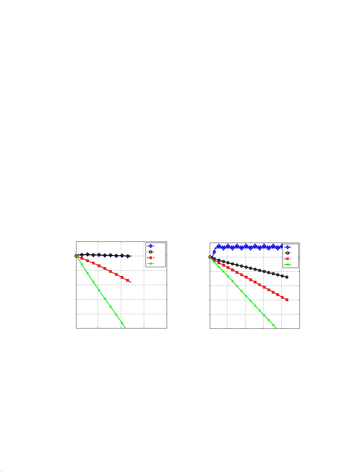
F ast global con v ergence of gr adien t metho ds for high-dimen sional statis tical rec o v ery Alekh Agarw al † Sahand N. Nega hban ‡ Martin J. W ain wrigh t ⋆, † alekh@ee cs.berke ley.edu sahandn@ mit.edu wainwrig @stat.be rkeley.e du Departmen t of Statistics ⋆ , and Departmen t of EECS ‡ , Departmen t of EECS † , Massac h usetts In stitute of T ec hnology , Univ ersit y of California, Berke ley 32 V assar Street Berk eley , CA 947 20-1776 Cam birdge MA 0213 9 Abstract Many sta tistical M -estimators a re bas ed o n conv ex o ptimization problems fo rmed b y the combination of a data-dep endent los s function with a norm-ba sed regular izer. W e analy ze the conv ergence rates of pro jected gradient and comp os ite gr adient methods for solving such prob- lems, working within a high-dimensional framework that allows the data dimension d to gr ow with (and po ssibly ex ceed) the sa mple size n . This high-dimensional s tr ucture prec ludes the usual global assumptions —namely , strong conv exity and s mo othness conditions—that underlie m uch of classical optimizatio n ana lysis. W e deﬁne appro pr iately restricted versions o f these conditions, and show that they a re satisﬁed with high proba bilit y for v arious statistical mo dels. Under these conditions, our theory guarantees that pr o jected gradie nt des c ent has a globa lly geometric rate of conv ergence up to the statistic al pr e cision o f the model, meaning the typical distance be tw een the tr ue unknown par ameter θ ∗ and a n optimal solution b θ . This r esult is substantially shar p er than previous co nv ergence results, which yielded sublinea r conv ergence, or linear co nv ergence only up to the nois e level. O ur a nalysis applies to a wide r a nge o f M - estimators and statistical mo dels, including spars e linear regr ession using Lass o ( ℓ 1 -regular ized regres s ion); gro up Lasso for blo ck sparsity; lo g-linear mo dels with r egulariza tion; low-rank ma - trix r ecov ery using nuclear norm r egulariza tion; a nd matrix deco mp o s ition. Overall, our analy - sis r e veals interesting connections betw een s tatistical pr ecision and computational eﬃciency in high-dimensional estimation. 1 In tro duction High-dimensional data sets presen t c hallenges th at are b oth stat istical an d computational in n atur e. On the statistical side, recen t y ears ha v e witnessed a ﬂur ry of r esults on consistency and rates for v arious estimators und er non-asymptotic high-dimens ional scaling, meaning that err or b oun ds are pro vided for general settings of the sample size n and problem dimension d , allo wing for the p ossibilit y that d ≫ n . These results t ypically inv olv e some assumption regarding the underlying structure of the parameter sp ace, suc h as sparse v ectors, structured co v ariance matrices, lo w-rank matrices, or structured regression functions, as wel l as some regularit y conditions on the d ata- generating pro cess. On the computational side, man y estimators for statistica l reco v ery are based on solving con v ex programs. Examples of suc h M -estimato rs include ℓ 1 -regularized quadratic programs (also kno wn as the L asso) for sparse linear r egression (e.g., see the p ap ers [41, 13, 45, 27, 6, 9, 43] and r eferen ces therein), second-order cone programs (SOCP) for the grou p Lasso (e.g., [46, 25, 20] and r eferences th erein), and semideﬁnite programming relaxations (SDP) for v arious problems, 1 including sparse P CA and lo w-rank matrix estimation (e.g., [11, 36, 40, 2, 38, 29, 37] and referen ces therein). Man y of these pr ograms are in stances of conv ex conic p r ograms, and so can (in p rinciple) b e solv ed to ǫ -accuracy in p olynomial time using interior p o int metho d s, and other s tandard metho ds from conv ex programming (e.g., see the b ooks [5, 7]). Ho w ev er, the complexit y of such quasi- Newton metho ds can b e pr ohibitiv ely exp ensive for the ve ry large-scale pr oblems that arise from high-dimensional data sets. Accordingly , recen t yea rs ha v e w itn essed a renewed interest in simpler ﬁrst-order metho ds, among them the metho d s of p ro jected gradien t d escen t and mirror descent. Sev eral au th ors (e.g., [4 , 21, 3]) h a v e u sed v arian ts of Nesterov’s accelerat ed gradien t m etho d [32] to obtain algorithms for h igh-dimensional statistical pr oblems with a sublin ear rate of conv ergence. Note that an optimization algorithm, generating a s equence of iterates { θ t } ∞ t =0 , is said to exhibit subline ar c onver genc e to an optim um b θ if the optimization error k θ t − b θ k deca ys at the rate 1 /t κ , for some exp onent κ > 0 and n orm k · k . Although this t yp e of con v ergence is quite slo w, it is the b est p o ssible with gradien t descen t-t yp e metho ds for conv ex pr ograms u nder only Lipsc hitz conditions [31]. It is kn own that muc h faster global rates—in particular, a linear or geometric rate—can b e ac hiev ed if global regularit y conditions like strong con v exit y and smo othness are imp o sed [31]. An optimization algorithm is said to exhibit line ar or ge ometric con v ergence if the optimization error k θ t − b θ k deca ys at a rate κ t , for some con traction co eﬃcien t κ ∈ (0 , 1). No te that suc h conv er- gence is exp onenti ally faster than su b-linear conv ergence. F or certain classes of pr oblems inv olving p olyhedral constraints and global smo othness, Tseng and Luo [26] ha v e established geometric con- v ergence. Ho wev er, a c hallenging asp ect of statistical estimation in high d imensions is that the underlying optimization problems can n ever b e strongly conv ex in a global sense wh en d > n (since the d × d Hessian matrix is rank-deﬁcien t), and global smo othness conditions cannot hold when d/n → + ∞ . Some more recen t wo rk has exploited str ucture s p eciﬁc to the optimization prob- lems that arise in statistical settings. F or the sp ecia l case of sp arse linear regression w ith rand om isotropic designs (also r eferred to as compressed sensing), some authors ha v e established fast con- v ergence r ates in a lo cal sense, m eanin g guaran tees that apply once the iterates are close en ou gh to the optim um [8 , 18 ]. The intuitio n underlying these results is that once an algorithm identiﬁes the supp ort set of the optimal solution, the pr ob lem is th en eﬀectiv ely reduced to a lo w er-dimensional subspace, and thus fast conv ergence can b e guarante ed in a lo cal sens e. Also in the setting of compressed sen s ing, T ropp and Gilb ert [42] studied ﬁn ite con ve rgence of greedy algorithms based on thresholding tec hniques, and show ed linear con v ergence u p to a certain tolerance. F or the same class of p r oblems, Garg and K h andek ar [17] sh o w ed that a thr esholded gradient algorithm con v erges rapidly up to some tolerance. In b ot h of these results, the con v ergence tolerance is of the order of the noise v ariance, and hence su bstan tially larger than the tr ue statistical pr ecision of the p roblem. The f o cus of this pap er is the con v ergence rate of t wo simp le gradien t-based algorithms for solv- ing optimization p roblems that und erlie r egularized M -estimators. F or a constrained p roblem with a diﬀerenti able ob jectiv e function, the pro jected gradien t metho d generates a s equ ence of iterates { θ t } ∞ t =0 b y taking a s tep in the negativ e gradien t d irection, and then pro jecting the result onto the constrain t set. The comp osite gradient metho d of Nestero v [32] is wel l-suited to solving regularized problems formed by the sum of a diﬀeren tiable and (p ote nti ally) non-diﬀerentiable comp onent. The main con tribution of this pap er is to establish a form of global geometric con v ergence for these algorithms that h olds for a br oad class of high-d im en sional statistical pr oblems. In ord er to pro vide in tuition for this guarant ee, Figure 1 sh o ws the p erformance of p ro jected gradien t descen t 2 for a Lasso problem ( ℓ 1 -constrained least-squares). In panel (a), w e ha ve plotted the logarithm of th e optimization error, measured in terms of the Euclidean n orm k θ t − b θ k b et ween the current iterate θ t and an optimal solution b θ , v ersus th e iteration n umb er t . The p lot includes three diﬀerent curv es, corresp onding to sparse regression problems in dimension d ∈ { 5000 , 10000 , 20000 } , and a ﬁxed sample size n = 2500. Note that all curves are linear (on this logarithmic scale), rev ealing the geometric con ve rgence p redicted by our th eory . Suc h conv ergence is not predicted by classi- cal optimization theory , s ince the ob jectiv e fun ction cannot b e strongly conv ex whenever n < d . Moreo v er, the con ve rgence is geometric eve n at early iterations, and take s place to a precision f ar less than the noise lev el ( ν 2 = 0 . 25 in this example). W e also note th at the design matrix do es not satisfy the r estricted isometry prop erty , as assumed in some past w ork. 50 100 150 −10 −8 −6 −4 −2 0 2 It era t i on Cou nt lo g( k θ t − ˆ θ k ) ( r esc al ed) n = 2 50 0 , ω = 0 . 2 5 , q = 0 d= 5000 d=10000 d=20000 50 100 150 −10 −8 −6 −4 −2 0 2 It era t i on Cou nt lo g( k θ t − ˆ θ k ) ( r esc al ed) α = 1 6 . 3 0 69 , ω = 0 . 2 5 , q = 0 d= 5000 d=10000 d=20000 (a) (b) Figure 1. Convergence rates of pr o jected gr a dient descent in application to L a sso progr a ms ( ℓ 1 - constrained least-s quares). Each pa nel shows the log optimiza tio n error lo g k θ t − b θ k versus the itera- tion num ber t . Panel (a) shows three curves, co rresp onding to dimensions d ∈ { 5 000 , 10000 , 20000 } , sparsity s = ⌈ √ d ⌉ , and all with the same sa mple size n = 25 00. All ca ses show geometric con- vergence, but the rate for la rger pr oblems b ecomes pro g ressively slow er. (b) F or an a ppropria tely rescaled sa mple size ( α = n s log d ), a ll three conv ergence r ates should be roughly the same, a s predicted by the theory . The r esults in panel (a) exhibit an in teresting pr op erty: the conv ergence rate is dimension- dep endent , meaning that for a ﬁ x ed sample size, pro jected gradient descent conv erges more slo wly for a large problem than a smaller pr oblem—compare the s q u ares for d = 20000 to the diamond s for d = 5000. T his phenomenon reﬂects the natural in tuition that larger p roblems are, in some sense, “harder” than smaller problems. A notable asp ect of our theory is that in addition to guarante eing geometric conv ergence, it makes a quantita tiv e prediction regarding the exten t to which a larger problem is harder than a sm aller one. In particular, our con ve rgence rates su ggest that if the sample size n is re-scaled in a certain w a y according to the d imension d and also other mo del parameters such as sp arsit y , then con v ergence rates sh ou ld b e r ou gh ly s imilar. P anel (b) pro vides a conﬁrmation of this pr ediction: wh en the samp le size is rescaled according to our theory (in particular, see Corollary 2 in Section 3.2), then all th ree curv es lie essen tially on top of another. Although h igh-dimensional op timization p roblems are typical ly neither strongly con v ex nor smo oth, this pap er shows that it is fru itful to consider su itably r estricted notions of strong con- 3 v exit y and smo o thness. Our notion of restricted strong conv exit y (RSC) is related to but sligh tly diﬀeren t than that in tro du ced in a recen t p ap er by Negah ban et al. [28] for establishin g statis- tical consistency . As we discus s in the sequel, b ound ing the optimization error int ro d uces new c hallenges not present when analyzing the statistical error. W e also introd uce a related n otion of restricted smo ot hn ess (RSM), n ot needed for pro ving statistical r ates but essen tial in the setting of optimization. O u r analysis consists of t w o p arts. W e ﬁ rst sho w that for optimization p r oblems underlying man y regularized M -estimators, app ropriately mo diﬁed notions of restricted strong con v exit y (RSC) and sm o othness (RSM) are suﬃ cien t to guaran tee global linear con v ergence of pro jected gradien t descent. Our second con tribution is to p ro v e that f or the iterates generated by our ﬁrst-order metho d, these RSC/RSM assumptions do ind eed h old w ith high pr obabilit y for a broad class of statistical mo dels, among them s parse linear mo dels, mo dels with group sparsity constrain ts, and v arious classes of matrix estimation problems, includ ing matrix completion and matrix decomp osition. An in teresting asp ec t of our resu lts is th at the global geometric con v ergence is n ot guaran teed to an arb itrary numerical precision, but only to an accuracy related to statistic al pr e cision of the pr oblem. F or a giv en error norm k · k , giv en by the Euclidean or F r ob enius n orm for most examples in this pap er, the statistical pr ecision is giv en by th e mean-squared error E [ k b θ − θ ∗ k 2 ] b et we en th e tru e parameter θ ∗ and the estimate b θ obtained by solving th e optimization p roblem, where the exp ectation is tak en o ve r randomn ess in the statistical mo d el. Note that th is is v ery natural from the statistical p ersp ective , since it is the true p arameter θ ∗ itself (as opp osed to the solution b θ of th e M -estimator) that is of primary inte rest, and our analysis allo ws us to approac h it as close as is statistically p ossible. Our analysis sho ws that w e can geometrically conv erge to a parameter θ suc h th at k θ − θ ∗ k = k b θ − θ ∗ k + o ( k b θ − θ ∗ k ), which is the b est we can h op e for statistically , ignoring lo w er order terms. Ov erall, our results r ev eal an inte resting connection b et we en the s tatistica l an d compu tational pr op erties of M -estimators—that is, th e prop erties of the un derlying statistical mo del th at mak e it fa vo rable f or estimation also render it more amenable to optimizati on pro cedures. The remainder of this pap er is organized as follo ws. W e b egi n in Section 2 with a precise form ulation of the class of con v ex programs analyzed in this pap er, along with bac kground on the notions of a decomp osable r egularizer, and prop erties of the loss function. Section 3 is dev oted to the s tatemen t of our m ain conv ergence result, as well as to th e d ev elopmen t and discus sion of its v arious corollaries f or sp eciﬁc statistical mo dels. In Section 4, we pr o vide a num b er of empirical results th at conﬁrm the sh arpness of our theoretical pr ed ictions. Finally , Section 5 conta ins th e pro ofs, with more tec hnical asp ects of the argum ents deferred to the App endix. 2 Bac kground and problem form ulation In this section, w e b egin b y describing th e class of r egularized M -estimators to which our analysis applies, as w ell as the optimization algorithms that we analyze. Finally , we introdu ce some im- p ortant notions th at under lie our analysis, including the notions of a decomp osable regularization, and the p rop erties of restricted strong conv exity and smo othness. 4 2.1 Loss functions, regularization and gradien t-based metho ds Giv en a random v ariable Z ∼ P taking v alues in some set Z , let Z n 1 = { Z 1 , . . . , Z n } b e a collecti on of n obs er v ations. Here the integ er n is the sample size of the p roblem. Assum ing that P lies within some ind exed family { P θ , θ ∈ Ω } , the goal is to r eco v er an estimate of the unkn o wn true parameter θ ∗ ∈ Ω generating the data. Here Ω is some subset of R d , and the integ er d is known as the ambient dimension of the p roblem. In ord er to measure the “ﬁt” of any giv en parameter θ ∈ Ω to a give n data set Z n 1 , we intro d uce a loss fun ction L n : Ω × Z n → R + . By construction, for an y giv en n -sample data set Z n 1 ∈ Z n , the loss fu nction assigns a cost L n ( θ ; Z n 1 ) ≥ 0 to the parameter θ ∈ Ω. I n many (but n ot all) applications, the loss function has a separable structure across the data set, meaning that L n ( θ ; Z n 1 ) = 1 n P n i =1 ℓ ( θ ; Z i ) where ℓ : Ω × Z : → R + is the loss fun ction asso ciated with a single d ata p oin t. Of p rimary interest in this p ap er are estimation problems th at are under-determin ed , meaning that the num b er of observ ations n is smaller than the am bient dimension d . In suc h settings, without furth er restrictions on the parameter sp ace Ω, there are v arious imp ossibilit y theorems, asserting th at consisten t estimates of the unknown p arameter θ ∗ cannot b e obtained. F or this reason, it is necessary to assume that th e unkn o wn parameter θ ∗ either lies within a smaller subset of Ω, or is w ell-appro ximated b y some mem b er of such a subset. In order to incorp orate these t yp es of structur al constrain ts, we in tro duce a r e gularizer R : Ω → R + o v er the p arameter space. With these ingredien ts, the analysis of th is p ap er applies to th e c onstr aine d M -estimator b θ ρ ∈ arg m in R ( θ ) ≤ ρ  L n ( θ ; Z n 1 ) } , (1) where ρ > 0 is a u ser-deﬁned radius, as well as to the r e gularize d M -estimator b θ λ n ∈ arg m in R ( θ ) ≤ ¯ ρ  L n ( θ ; Z n 1 ) + λ n R ( θ ) | {z } φ n ( θ )  (2) where th e regularization wei ght λ n > 0 is user-deﬁ n ed. Note that the radii ρ and ¯ ρ may b e diﬀerent in general. Throu gh ou t this pap er, w e imp ose the follo wing t w o conditions: (a) for an y data set Z n 1 , th e fu nction L n ( · ; Z n 1 ) is conv ex and diﬀeren tiable o ve r Ω, and (b) the regularizer R is a norm. These conditions ens u re that the o v erall problem is conv ex, so th at by Lagrangian dualit y , the optimization problems (1) and (2) are equiv alen t. How ev er , as our analysis will show, solving one or the other can b e computationally more preferable dep end ing up on the assump tions made. Some remarks on notation: wh en the r adius ρ or the r egularizatio n parameter λ n is clear f rom the con text, w e will drop the subscrip t on b θ to ease the n otation. Similarly , we frequently adopt the sh orthand L n ( θ ), with the dep endence of th e loss fun ction on the data b eing implicitly un d ersto o d. Pr o cedures based on optimization problems of either form are kn o wn as M -estimators in the statistics literature. The fo cus of this pap er is on tw o simple algorithms for solving the ab o ve optimizatio n p roblems. The m etho d of pr oje cte d gr adient desc ent applies naturally to the constrained pr oblem (1), wh ereas the c omp osite g r adient desc ent metho d due to Nestero v [32] is su itable for s olving the regularized 5 problem (2). Eac h routine generates a sequ ence { θ t } ∞ t =0 of iterates by ﬁ rst in itializing to s ome parameter θ 0 ∈ Ω , and then applying the recursiv e up date θ t +1 = arg min θ ∈ B R ( ρ )  L n ( θ t ) + h∇L n ( θ t ) , θ − θ t i + γ u 2 k θ − θ t k 2  , for t = 0 , 1 , 2 , . . . , (3) in the case of pr o jecte d gradien t descent, or the up date θ t +1 = arg min θ ∈ B R ( ¯ ρ )  L n ( θ t ) + h∇L n ( θ t ) , θ − θ t i + γ u 2 k θ − θ t k 2 + λ n R ( θ )  , for t = 0 , 1 , 2 , . . . , (4) for the comp osite gradien t metho d . Not e that the only diﬀeren ce b et ween the t w o up dates is the addition of the regularization term in the ob jectiv e. These up dates hav e a n atural int uition: the next iterate θ t +1 is obtained b y constrained minimization of a ﬁrst-order appro ximation to the loss function, com bined with a smo ot hing term that controls ho w far one mov es fr om the cur ren t iterate in terms of Eu clidean n orm. Moreo v er, it is easily seen that the up date (3) is equiv alen t to θ t +1 = Π  θ t − 1 γ u ∇L n ( θ t )  , (5) where Π ≡ Π B R ( ρ ) denotes Euclidean pro jection onto the b all B R ( ρ ) = { θ ∈ Ω | R ( θ ) ≤ ρ } of radius ρ . In th is f orm ulation, we see that the algorithm tak es a step in the negativ e gradient direction, u sing the qu an tit y 1 /γ u as stepsize parameter, and then pro jects the r esu lting ve ctor on to the constrain t set. The up date (4) take s an analogous form, ho w ev er, the pro jection will dep end on b oth λ n and γ u . As will b e illustrated in the examples to follo w, f or man y problems, the up d ates (3) and (4), or equ iv alen tly (5), hav e a very simp le solution. F or instance, in the case of ℓ 1 -regularizatio n, it can b e obtained b y an app ropriate form of the soft-thresholdin g op erato r. 2.2 Restricted strong con v exit y and smo othness In th is section, w e deﬁn e the conditions on the loss fun ction and regularizer that und erlie our analysis. Global smo othness an d s trong conv exit y assumptions play an imp ortan t role in the classical analysis of optimization algorithms [5, 7, 31]. I n app lication to a diﬀerenti able loss function L n , b ot h of these prop erties are deﬁned in terms of a ﬁrst-order T a ylor series exp ansion around a v ector θ ′ in the dir ection of θ —namely , the quan tit y T L ( θ ; θ ′ ) := L n ( θ ) − L n ( θ ′ ) − h∇L n ( θ ′ ) , θ − θ ′ i . (6) By the assumed conv exit y of L n , this error is alw a ys n on-negativ e, and global str ong con ve xit y is equiv alen t to imp osing a stronger condition, namely that for some parameter γ ℓ > 0, the ﬁrst- order T a ylor error T L ( θ ; θ ′ ) is lo w er b ounded b y a quadr atic term γ ℓ 2 k θ − θ ′ k 2 for all θ , θ ′ ∈ Ω . Global smo othness is deﬁned in a similar w a y , by imp osing a q u adratic u pp er b oun d on the T a ylor error. It is kn o wn that under global smo othn ess and str on g conv exity assumptions, the metho d of pro jected gradient descen t (3) en j o ys a glob al ly ge ometric c onver genc e r ate , m eanin g that there is some κ ∈ (0 , 1) such that 1 k θ t − b θ k 2 . κ t k θ 0 − b θ k 2 for all iterations t = 0 , 1 , 2 , . . . . (7) 1 In this statement (and th roughout the pap er), w e use . to mean an ineq ualit y that h olds with some universal constant c , indep endent of the problem parameters. 6 W e refer the reader to Bertsek as [5, P rop. 1.2.3, p. 145] , or Nestero v [31, Thm. 2.2.8, p. 88] for suc h results on p ro jected gradient descen t, and to Nestero v [32] f or comp osite gradient descen t. Unfortunately , in the high-d imensional setting ( d > n ), it is usually imp ossib le to guaran tee strong con ve xit y of the pr oblem (1) in a global sen s e. F or in stance, wh en the data is dra wn i.i.d., the loss function consists of a sum of n terms. If the loss is t wice diﬀeren tiable, the resulting d × d Hessian matrix ∇ 2 L ( θ ; Z n 1 ) is often a sum of n matrices eac h with rank one, so th at the Hessian is rank-degenerate w hen n < d . Ho w ev er, as w e sho w in this pap er, in ord er to obtain fast conv er - gence rates f or the optimization metho d (3) , it is suﬃcient th at (a) the ob jectiv e is strongly con v ex and smo oth in a restricted set of directions, and (b) the algorithm approac hes the optimum b θ only along th ese directions. Let us no w formalize these ideas. Deﬁnition 1 ( Restricted strong con v exit y (RSC)) . The loss function L n satisﬁes r estricte d str ong c onvexity with r esp e ct to R and with p ar ameters ( γ ℓ , τ ℓ ( L n )) over the set Ω ′ if T L ( θ ; θ ′ ) ≥ γ ℓ 2 k θ − θ ′ k 2 − τ ℓ ( L n ) R 2 ( θ − θ ′ ) for al l θ , θ ′ ∈ Ω ′ . (8) W e refer to the quan tit y γ ℓ as the (lower) cu rvatur e p ar ameter , and to the quantit y τ ℓ as the toler anc e p ar ameter . The set Ω ′ corresp onds to a su itably chosen subset of the sp ace Ω of all p ossible parameters. In ord er to gain intuitio n for this deﬁn ition, ﬁ rst su pp ose that the condition (8) holds with tolerance parameter τ ℓ = 0. In th is case, the r egularizer pla ys no role in the deﬁn ition, and condition (8) is equiv alen t to the u sual deﬁnition of strong con v exit y on the optimization set Ω. As discussed previously , th is t yp e of global strong conv exity typical ly fails to hold for high-dimensional inference problems. In con trast, wh en tolerance parameter τ ℓ is strictly p ositiv e, the condition (8) is muc h milder, in that it only app lies to a limite d set of v ectors. F or a giv en pair θ 6 = θ ′ , consider the inequalit y R 2 ( θ − θ ′ ) k θ − θ ′ k 2 < γ ℓ 2 τ ℓ ( L n ) . (9) If this inequalit y is violated, th en the righ t-hand sid e of the b oun d (8) is non-p ositive , in which case the RSC constraint (8) is v acuous. Thus, restricted strong con v exit y imp oses a non-trivial constrain t only on pairs θ 6 = θ ′ for wh ic h the inequalit y (8) holds, and a cen tral part of our analysis will b e to pro v e that, for the sequence of iterates generated by pro jected gradient descent, the optimization error b ∆ t := θ t − b θ satisﬁes a constraint of the f orm (9) . W e note that s ince th e regularizer R is conv ex, strong con v exit y of the loss fun ction L n also implies the strong con v exit y of the r egularized loss φ n as w ell. F or the least-squares loss, the RS C d eﬁnition dep en ds pu r ely on the direction (and not th e magnitude) of th e diﬀerence v ector θ − θ ′ . F or other t yp es of loss f unctions—such as those arising in generalized linear mo dels—it is essenti al to lo calize th e RSC deﬁnition, requiring that it holds only for pairs for whic h th e norm k θ − θ ′ k 2 is not to o large. W e refer the r eader to S ection 2.4.1 for further d iscussion of this iss ue. Finally , as p oin ted out by a review er, our restricted version of strong conv exity can b e seen as an instance of the general theory of paracon v exit y (e.g., [33]); ho w ev er, we are not a wa re of con v ergence rates for minimizing general paracon v ex fun ctions. W e also sp ec ify an analog ous notion of r estricted smo othness: 7 Deﬁnition 2 ( Restricted smoothne ss (RSM)). We say the loss function L n satisﬁes r estricte d smo othness with r esp e ct to R and with p ar ameters ( γ u , τ u ( L n )) over the set Ω ′ if T L ( θ ; θ ′ ) ≤ γ u 2 k θ − θ ′ k 2 + τ u ( L n ) R 2 ( θ − θ ′ ) for al l θ , θ ′ ∈ Ω ′ . (10) As with our d eﬁnition of restricted strong conv exit y , the additional tolerance τ u ( L n ) is not pr esen t in analogous smo othness conditions in the optimizatio n literature, but it is essen tial in our set-up. 2.3 Decomp osable regularizers In past work on the statistical pr op erties of regularization, th e notion of a decomp o sable regularizer has b een sh o wn to b e usefu l [28]. Although the fo cus of this pap er is a r ather diﬀerent set of questions—namely , optimization as opp osed to statistics—decomp osabilit y also p la ys an imp ortan t role here. Decomp osabilit y is deﬁned with resp ect to a pair of su b spaces deﬁn ed w ith r esp ect to the parameter s p ace Ω ⊆ R d . The set M is kno wn as the mo del su bsp ac e , whereas the set M ⊥ , referred to as the p erturb ation subsp ac e , captures deviations a wa y from the mo del subsp ace. Deﬁnition 3. Given a subsp ac e p air ( M , M ⊥ ) such that M ⊆ M , we say that a norm R is ( M , M ⊥ ) - decomp osable if R ( α + β ) = R ( α ) + R ( β ) for al l α ∈ M and β ∈ M ⊥ . (11) T o gain some intuitio n for this deﬁn ition, note that by triangle in equ alit y , we alw a ys ha v e the b ound R ( α + β ) ≤ R ( α ) + R ( β ). F or a decomp osable regularizer, this inequalit y alw a ys h olds with equalit y . Thus, give n a ﬁxed v ector α ∈ M , the key prop ert y of any decomp osable r egularizer is that it aﬀords the maximum p enalizatio n of an y deviation β ∈ M ⊥ . F or a giv en error norm k · k , its in teraction with the regularizer R pla ys an imp ortant role in our results. In particular, w e ha v e the follo wing: Deﬁnition 4 (S ubspace compatibilit y) . Given the r e gularizer R ( · ) and a norm k · k , the asso ciate d subspace compatibilit y is given by Ψ( M ) := sup θ ∈ ¯ M\{ 0 } R ( θ ) k θ k when M 6 = { 0 } , and Ψ( { 0 } ) := 0 . (12) The quantit y Ψ( M ) corresp onds to the Lipschitz constant of the n orm R with r esp ect to k · k , when restricted to the s u bspace M . 2.4 Some illustrative examples W e now describ e s ome particular examples of M -estimators with decomp osable r egularizers, and discuss the form of th e pro jected gradien t up dates as w ell as RSC/RS M cond itions. W e cov er t w o main families of examples: log-li near mo d els with sparsit y constrain ts and ℓ 1 -regularizatio n (Section 2.4.1), and matrix r egression p r oblems with nuclear n orm regularizatio n (Section 2.4.2). 8 2.4.1 Sparse log-linear mo dels and ℓ 1 -regularization Supp ose that eac h sample Z i consists of a scalar-v ector pair ( y i , x i ) ∈ R × R d , corresp onding to the scalar resp onse y i ∈ Y associated with a vecto r of p redictors x i ∈ R d . A log-linear m o del with canonical link fun ction assumes that the resp onse y i is linked to the co v ariate v ector x i via a conditional distrib ution of the form P ( y i | x i ; θ ∗ , σ ) ∝ exp  y i h θ ∗ , x i i− Φ( h θ ∗ , x i i ) c ( σ )  , where c ( σ ) is a known quanti t y , Φ( · ) is the log-partition f unction to normalize the den s it y , and θ ∗ ∈ R d is an unknown regression vecto r. In man y app lications, the regression vec tor θ ∗ is relativ ely sparse, so that it is n atural to imp ose an ℓ 1 -constrain t. Computing the maxim um like liho o d estimate sub ject to suc h a constrain t in v olv es solving the con v ex pr ogram 2 b θ ∈ arg min θ ∈ Ω n 1 n n X i =1  Φ( h θ , x i i ) − y i h θ , x i i  | {z } L n ( θ ; Z n 1 ) o suc h that k θ k 1 ≤ ρ , (13) with x i ∈ R d as its i th ro w. W e refer to th is estimator as the log-linear L asso; it is a sp ecial case of the M -estimator (1), with the loss fun ction L n ( θ ; Z n 1 ) = 1 n P n i =1  Φ( h θ , x i i ) − y i h θ , x i i  and the regularizer R ( θ ) = k θ k 1 = P d j =1 | θ j | . Ordinary linear regression is the sp eci al case of the log-linear setting with Φ( t ) = t 2 / 2 and Ω = R d , and in this case, the estimator (1 3) corresp on d s to ordinary least-squares version of Lasso [13, 41]. Other forms of log-linear Lasso that are of interest includ e logistic regression, P oisson regression, and m ultinomial regression. Pro jected gradien t up da t es: Computing the gradient of the log-linear loss fr om equation (13 ) is straight forward: w e ha ve ∇ L n ( θ ) = 1 n P n i =1 x i  Φ ′ ( h θ , x i i ) − y i  , and th e up date (5) corresp onds to th e Eu clidean pro jection of the v ector θ t − 1 γ u ∇L n ( θ t ) on to the ℓ 1 -ball of radiu s ρ . It is well- kno wn that this pr o jecti on can b e charac terized in terms of soft-thresh oldin g, and th at the pro- jected u p date (5) can b e compu ted easily . W e refer the r eader to Duchi et al. [14] for an eﬃcient implemen tation requirin g O ( d ) op erations. Comp osite gradient up dates: The comp osite gradien t up date for th is pr oblem amounts to solving θ t +1 = arg min k θ k 1 ≤ ¯ ρ n h θ , ∇L n ( θ ) i + γ u 2 k θ − θ t k 2 2 + λ n k θ k 1 o . The up date can b e compu ted b y t w o soft-thresholding op erations. T he ﬁr st step is soft thr esolding the v ector θ t − 1 γ u ∇L n ( θ t ) at a level λ n . If the resulting ve ctor has ℓ 1 -norm greater than ¯ ρ , then w e pr o ject on to the ℓ 1 -ball just like b efore. Overall, the complexit y of the up date is still O ( d ) as b efore. Decomp osabilit y of ℓ 1 -norm: W e now illustrate how the ℓ 1 -norm is decomp osable with resp ect to appropriately c hosen subsp aces. F or any subset S ⊆ { 1 , 2 , . . . , d } , consider th e su bspace M ( S ) :=  α ∈ R d | α j = 0 for all j / ∈ S } , (14) 2 The link function Φ is conv ex since it is th e log-partition function of a canon ical exp onential family . 9 corresp ondin g to all vect ors supp orted only on S . Deﬁning M ( S ) = M ( S ), its orthogonal comple- men t (with resp ect to the u sual Euclidean inner p r o duct) is given by M ⊥ ( S ) = M ⊥ ( S ) =  β ∈ R d | β j = 0 for all j ∈ S  . (15) T o establish the decomp o sabilit y of the ℓ 1 -norm with resp ect to the p air ( M ( S ) , M ⊥ ( S )), n ote th at an y α ∈ M ( S ) can b e w ritten in the p artitioned form α = ( α S , 0 S c ), w here α S ∈ R s and 0 S c ∈ R d − s is a vect or of zeros. Similarly , an y v ector β ∈ M ⊥ ( S ) has the p artitioned represen tation (0 S , β S c ). With these represen tations, w e ha v e the decomp osition k α + β k 1 = k ( α S , 0) + (0 , β S c ) k 1 = k α k 1 + k β k 1 . Consequent ly , for an y subset S , the ℓ 1 -norm is decomp osable with resp ect to the pairs ( M ( S ) , M ⊥ ( S )). In an alogy to the ℓ 1 -norm, v arious t yp es of group -sparse n orms are also decomp o sable with resp ect to non -trivial su bspace pairs. W e refer the reader to the p ap er [28] for fu rther discussion and examples of su ch decomp o sable norms. RSC/RSM conditions: A calculation usin g the mean-v alue theorem shows that for the loss function (13), the err or in the ﬁrst-order T a ylor series, as pr eviously deﬁned in equation (6), can b e written as T L ( θ ; θ ′ ) = 1 n n X i =1 Φ ′′  h θ t , x i i   h x i , θ − θ ′ i  2 where θ t = tθ + (1 − t ) θ ′ for s ome t ∈ [0 , 1]. When n < d , then w e can alw a ys ﬁnd pairs θ 6 = θ ′ suc h that h x i , θ − θ ′ i = 0 for all i = 1 , 2 , . . . , n , showing that the ob jectiv e fun ction can nev er b e strongly con ve x. O n the other hand, restricted strong conv exity for log-linear mo dels requires only that there exist p ositiv e n umbers ( γ ℓ , τ ℓ ( L n )) suc h that 1 n n X i =1 Φ ′′  h θ t , x i i   h x i , θ − θ ′ i  2 ≥ γ ℓ 2 k θ − θ ′ k 2 − τ ℓ ( L n ) R 2 ( θ − θ ′ ) for all θ , θ ′ ∈ Ω ′ , (16) where Ω ′ := Ω ∩ B 2 ( R ) is the intersecti on of the parameter space Ω w ith a Eu clidean ball of some ﬁxed radiu s R around zero. Th is restriction is essential b ecause for m an y generalized lin ear mo d els, the Hessian fu nction Φ ′′ approac hes zero as its argument diverges. F or in stance, for the logistic function Φ ( t ) = log(1 + exp( t )), we ha ve Φ ′′ ( t ) = exp( t ) / [1 + exp( t )] 2 , whic h tends to zero as t → + ∞ . Restricted smo othness imp oses an analogous up p er b ound on the T a ylor error. F or a broad class of log-linea r mo d els, such b ounds hold with tolerance τ ℓ ( L n ) and τ u ( L n ) of the ord er q log d n . F u r ther details on suc h results are pr o vided in the corollaries to follo w our main theorem. A d etailed discus s ion of RSC for exp onen tial families in statistical problems can b e f ound in the pap er [28]. In order to ensure RSC/RSM conditions on the iterates θ t of the u p d ates (3) or (4), we also need to ensu re that θ t ∈ Ω ′ . This can b e done by deﬁning L ′ n = L n + I Ω ′ ( θ ), wh er e I Ω ′ ( θ ) is zero when θ ∈ Ω ′ and ∞ otherwise. Th is is equiv alen t to p ro jectio n on the in tersection of ℓ 1 -ball w ith Ω ′ in the up dates (3) and (4) and can b e done eﬃcient ly with Dykstra’s algorithm [15], for in stance, as long as the individ ual p ro jectio ns are eﬃcien t. 10 In the sp ecial case of linear regression, w e hav e Φ ′′ ( t ) = 1 for all t ∈ R , s o that the lo w er b ound (16) inv olv es only the Gram matrix X T X/n . (Here X ∈ R n × d is the usual d esign m atrix, with x i ∈ R d as its i th ro w.) F or lin ear r egression and ℓ 1 -regularizatio n, the RSC condition is equiv alent to the lo w er b ound k X ( θ − θ ′ ) k 2 2 n ≥ γ ℓ 2 k θ − θ ′ k 2 2 − τ ℓ ( L n ) k θ − θ ′ k 2 1 for all θ , θ ′ ∈ Ω . (17) Suc h a condition corresp onds to a v ariant of the restricted eigen v alue (RE) conditions th at h a v e b een studied in the literature [6, 43]. Such RE conditions are signiﬁcan tly milder than the restricted isometry prop ert y; w e refer the reader to v an de Geer and Buh lmann [43] for an in -d epth comparison of diﬀerent RE conditions. F rom past work, the condition (17 ) is satisﬁed with high probabilit y for a broad classes of anisotropic random design matrices [34, 39], and parts of our analysis mak e use of this fact. 2.4.2 Matrices and n uclear norm regularization W e now discuss a general class of matrix r egression p roblems th at falls within our framewo rk. Consider the space of d 1 × d 2 matrices endo we d with the trace inn er p ro duct h h A , B i i := trace( A T B ). In order to ease notation, we deﬁn e d := min { d 1 , d 2 } . Let Θ ∗ ∈ R d 1 × d 2 b e an unknown matrix and supp ose that for i = 1 , 2 , . . . , n , we observ e a scalar-matrix pair Z i = ( y i , X i ) ∈ R × R d 1 × d 2 link ed to Θ ∗ via the linear mo d el y i = h h X i , Θ ∗ i i + w i , for i = 1 , 2 , . . . , n, (18) where w i is an additive observ ation noise. In man y con texts, it is natural to assume that Θ ∗ is exactly low-rank, or app ro ximately so, meaning that it is we ll-approxima ted by a matrix of low rank. In suc h settings, a n umber of authors (e.g., [16, 38, 29]) ha v e stu d ied the M -estimator b Θ ∈ arg min Θ ∈ R d 1 × d 2 n 1 2 n n X i =1  y i − h h X i , Θ i i  2 o suc h that | | | Θ | | | 1 ≤ ρ , (19) or the corresp onding regularized version. Here the nu c le ar or tr ac e norm is giv en b y | | | Θ | | | 1 := d P j =1 σ j (Θ), corresp ondin g to the su m of the singular v alues. This optimization problem is an instance of a semideﬁnite program. As d iscu ssed in more detail in Section 3.3, there are v arious applications in whic h this estimator and v arian ts thereof ha ve p ro v en useful. F orm of pro jected gradient descent: F or the M-estimato r (19), the p ro jected gradient up dates tak e a v ery simple form—namely Θ t +1 = Π  Θ t − 1 γ u P n i =1  y i − h h X i , Θ t i i  X i n  , (20) where Π denotes Euclidean pro jectio n onto the n uclear norm b all B 1 ( ρ ) = { Θ ∈ R d 1 × d 2 | | | | Θ | | | 1 ≤ ρ } . This nuclea r norm pr o jecti on can b e obtained by ﬁ rst computing the singu lar v alue decomp osition (SVD), and then pro jecting the ve ctor of sin gu lar v alues on to th e ℓ 1 -ball. The latter s tep can b e ac hiev ed by the fast pro jection algorithms discussed earlier, an d there are v arious metho ds for fast computation of SVDs. T he comp osite gradien t up date also has a simple form, requirin g at most t w o singular v alue thr esholding op erations as was the case for linear regression. 11 Decomp osabilit y of n uclear norm: W e n o w d eﬁ ne matrix subs p aces for whic h the nuclear norm is decomp osable. Given a target matrix Θ ∗ —that is, a quantit y to b e estimated—consider its singular v alue d ecomp osition Θ ∗ = U DV T , wh er e the matrix D ∈ R d × d is diagonal, with the ordered singular v alues of Θ ∗ along its diagonal, and d := min { d 1 , d 2 } . F or an in teger r ∈ { 1 , 2 , . . . , d } , let U r ∈ R d × r denote the matrix f orm ed b y the top r left singular v ectors of Θ ∗ in its columns , and w e deﬁne the matrix V r in a similar fashion. Using col to denote the column span of a matrix, we then deﬁne the su bspaces 3 M ( U r , V r ) :=  Θ ∈ R d 1 × d 2 | col(Θ T ) ⊆ col( V r ) , col(Θ) ⊆ col( U r )  , and (21a) M ⊥ ( U r , V r ) :=  Θ ∈ R d 1 × d 2 | col(Θ T ) ⊆ (col( V r )) ⊥ , col(Θ ) ⊆ (col( U r )) ⊥  . (21b) Finally , let u s ve rify the d ecomp osabilit y of the nucle ar norm . By construction, any pair of matrices Θ ∈ M ( U r , V r ) and Γ ∈ M ⊥ ( U r , V r ) h a v e orth ogonal row and column s p aces, whic h implies th e required decomp osabilit y condition—namely | | | Θ + Γ | | | 1 = | | | Θ | | | 1 + | | | Γ | | | 1 . In some sp ecial cases suc h as matrix completion or matrix decomp osition that we describ e in the sequel, Ω ′ will in vo lv e an additional b ound on the entries of Θ ∗ as w ell as the iterates Θ t to establish RSC/RSM conditions. Th is can b e done by augmenting the loss with an indicator of the constrain t and using cyclic pro jecti ons for computing the up d ates as men tioned earlier in Example 2.4.1. 3 Main results and some consequences W e are now equipp ed to state the tw o main results of our pap er, an d d iscuss some of th eir con- sequences. W e illustr ate its application to seve ral statistical mo d els, in cluding s parse regression (Section 3.2), matrix estimation with rank constraints (S ection 3.3), and m atrix decomp osition problems (Section 3.4). 3.1 Geometric con v ergence Recall that the pro jected gradien t algorithm (3) is well -suited to solving an M -est imation problem in its constrained form, w h ereas th e comp osite gradien t algorithm (4) is ap p ropriate f or a regular- ized pr ob lem. Accordingly , let b θ b e an y optimal solution to the constrained problem (1), or the regularized problem (2), and let { θ t } ∞ t =0 b e a sequ ence of iterates generated by generated by the pro jected gradient up dates (3), or the the comp osite gradien t up dates (4), resp ectiv ely . Of primary in terest to us in this pap er are b oun ds on th e optimization err or , wh ic h can b e measured either in terms of the error v ector b ∆ t := θ t − b θ , or the diﬀerence b et wee n the cost of θ t and the optimal cost deﬁned b y b θ . In this section, we state tw o main results —-Theorems 1 and 2—corresp onding to the constrained and regularized cases r esp ectiv ely . In addition to the optimization error previously discussed, b oth of th ese results inv olv e the statistic al err or ∆ ∗ := b θ − θ ∗ b et we en th e optim um b θ and the nominal parameter θ ∗ . A t a high leve l, these resu lts guarantee th at und er the RSC /RSM conditions, the optimization error shrinks geometrically , w ith a cont raction co eﬃcient that dep end s on the the loss function L n via the p arameters ( γ ℓ , τ ℓ ( L n )) and ( γ u , τ u ( L n )). An inte resting feature is that the con traction o ccurs only u p to a certain tolerance ǫ 2 dep end ing on these same parameters, and the statistica l error. How ever, as w e d iscu ss, for man y statistical pr oblems of interest, w e can 3 Note that the mo del space M ( U r , V r ) is not e qual to M ( U r , V r ). N on et h eless, as req uired by Deﬁnition 3, we do hav e the inclusion M ( U r , V r ) ⊆ M ( U r , V r ). 12 sho w that this tolerance ǫ 2 is of a low er order than th e intrinsic statistical error, and h ence can b e n eglecte d from the statistical p oint of view. C onsequen tly , our theory giv es an explicit upp er b ound on the num b er of iterations requir ed to solv e an M -estimatio n problem up to the statistical precision. Con v ergence rates for pro jected gradien t: W e n o w p r o vide the notation necessary for a precise statemen t of this claim. Our main r esult actually in v olv es a family of upp er b ou n ds on the optimization error, one for eac h pair ( M , M ⊥ ) of R -decomp osable sub spaces (see Deﬁn ition 3). As will b e clariﬁed in the sequel, this sub space choic e can b e optimized for diﬀeren t mo d els s o as to obtain the tigh test p ossible b ound s. F or a giv en pair ( M , M ⊥ ) su c h that 16Ψ 2 ( M ) τ u ( L n ) < γ u , let us d eﬁne the c ontr action c o eﬃcient κ ( L n ; M ) := n 1 − γ ℓ γ u + 16Ψ 2 ( M )  τ u ( L n ) + τ ℓ ( L n )  γ u o n 1 − 16Ψ 2 ( M ) τ u ( L n ) γ u o − 1 . (22) In addition, we d eﬁne the toler anc e p ar ameter ǫ 2 (∆ ∗ ; M , M ) := 32  τ u ( L n ) + τ ℓ ( L n )   2 R (Π M ⊥ ( θ ∗ )) + Ψ( M ) k ∆ ∗ k + 2 R (∆ ∗ )  2 γ u , (23) where ∆ ∗ = b θ − θ ∗ is the statistical error, and Π M ⊥ ( θ ∗ ) denotes the Euclidean pro jection of θ ∗ on to the subspace M ⊥ . In terms of these t wo ingred ien ts, w e no w state our ﬁrst main r esult: Theorem 1. Supp ose that the loss f u nction L n satisﬁes the RSC/RSM c ondition with p ar ameters ( γ ℓ , τ ℓ ( L n )) and ( γ u , τ u ( L n )) r esp e ctively. L et ( M , M ) b e any R -de c omp osable p air of subsp ac es such that M ⊆ M and 0 < κ ≡ κ ( L n , M ) < 1 . Then for any optimum b θ of the pr oblem (1) f or which the c onstr aint is active, we have k θ t +1 − b θ k 2 ≤ κ t k θ 0 − b θ k 2 + ǫ 2 (∆ ∗ ; M , M ) 1 − κ for al l iter ations t = 0 , 1 , 2 , . . . . (24) Remarks: Th eorem 1 actually pro vides a family of upp er b oun ds, one for eac h R -decomp osable pair ( M , M ) such that 0 < κ ≡ κ ( L n , M ) < 1. This condition is alw a ys satisﬁed by setting M equal to th e trivial su bspace { 0 } : indeed, by deﬁnition (12) of the su b space compatibilit y , we ha v e Ψ( M ) = 0, and hence κ ( L n ; { 0 } ) =  1 − γ ℓ γ u  < 1. Although this c hoice of M minimizes the con traction co eﬃcien t, it will lead 4 to a very large tolerance parameter ǫ 2 (∆ ∗ ; M , M ). A more t ypical application of Theorem 1 inv olv es non-trivial c hoices of the subspace M . The b ound (24) guarantee s that th e optimization error decreases geometrically , with contrac - tion f actor κ ∈ (0 , 1), up to a certain tolerance p r op ortional to ǫ 2 (∆ ∗ ; M , M ), as illus trated in Figure 2(a). The contract ion factor κ approac hes the 1 − γ ℓ /γ u as the n umb er of samples gro ws. The ap p earance of the ratio γ ℓ /γ u is natural s in ce it measures the conditioning of the ob jectiv e function; more sp eciﬁcally , it is essentia lly a restricted condition num b er of th e Hessian m atrix. O n 4 Indeed, the setting M ⊥ = R d means that the term R (Π M ⊥ ( θ ∗ )) = R ( θ ∗ ) app ears in the tolerance; this quantit y is far larger than statistical precision. 13 the other hand , the tolerance parameter ǫ dep end s on th e c hoice of decomp osable su bspaces, th e parameters of th e RS C/RSM conditions, and the statistica l err or ∆ ∗ = b θ − θ ∗ (see equation (23)). In the corollaries of T heorem 1 to follo w, we sh o w that the su b spaces can often b e c hosen su ch that ǫ 2 (∆ ∗ ; M , M ) = o ( k b θ − θ ∗ k 2 ). C onsequen tly , the b ound (24) guarantees geometric con v ergence u p to a tolerance smal ler than statistic al pr e cision , as illustr ated in Figure 2(b). Th is is sensible, since in statistic al settings, there is no p oin t to optimizing b ey ond the statistical precision. b ∆ 0 b ∆ 1 b ∆ t 0 ǫ b ∆ 0 b ∆ 1 b ∆ t 0 ǫ k ∆ ∗ k ∆ ∗ (a) (b) Figure 2. (a) Gener ic illustr ation of Theorem 1. The optimizatio n err o r b ∆ t = θ t − b θ is gua r anteed to decrease g eometrically with co eﬃcient κ ∈ (0 , 1 ), up to the to lerance ǫ 2 = ǫ 2 (∆ ∗ ; M , M ), represented by the circle. (b) Relation be tw een the optimizatio n tolerance ǫ 2 (∆ ∗ ; M , M ) (solid circle) and the statistical precisio n k ∆ ∗ k = k θ ∗ − b θ k (dotted c ircle). In many settings, we ha ve ǫ 2 (∆ ∗ ; M , M ) ≪ k ∆ ∗ k 2 , so tha t c onv ergence is guaranteed up to a to le r ance low er tha n statistical precision. The result of Th eorem 1 takes a simpler form w hen there is a su b space M that includes θ ∗ , an d the R -ball radius is c hosen s uc h that ρ ≤ R ( θ ∗ ). In this case, b y appr opriately controll ing the error term, we can establish that it is of lo w er order than the statistic al precision —n amely , the squared diﬀerence k b θ − θ ∗ k 2 b et we en an optimal solution b θ to the con v ex pr ogram (1), and th e un kno wn parameter θ ∗ . Corollary 1. In addition to the c onditio ns of The or em 1, supp ose that θ ∗ ∈ M and ρ ≤ R ( θ ∗ ) . Then as long as Ψ 2 ( M )  τ u ( L n ) + τ ℓ ( L n )  = o (1) , we have k θ t +1 − b θ k 2 ≤ κ t k θ 0 − b θ k 2 + o  k b θ − θ ∗ k 2  for al l iter ations t = 0 , 1 , 2 , . . . . (25) Th us, Corollary 1 guaran tees that the optimization err or d ecreases geometrically , with con tractio n factor κ , up to a tolerance that is of strictly lo w er order than the statistical precision k b θ − θ ∗ k 2 . As will b e clariﬁed in s everal examples to follo w, the condition Ψ 2 ( M )  τ u ( L n ) + τ ℓ ( L n )  = o (1) is satisﬁed f or many statistical mo d els, in clud ing spars e linear regression and lo w-rank matrix re- gression. T his r esult is illustrated in Figure 2(b), where the solid circle represents the optimization tolerance, and th e dotted circle represents the statistical precision. In the results to follo w, we will quan tify the term o  k b θ − θ ∗ k 2  in a more precise manner for diﬀeren t statistical mo dels. 14 Con v ergence rat e s for comp osite gradien t: W e now present our main result for the comp osit e gradien t iterates (4 ) that are suitable for the Lagrangian-based estimator (2). As b efore, our analysis yields a range of b ounds indexed by sub space pairs ( M , M ⊥ ) th at are R -decomp osa ble. F or any subspace M s u c h that 64 τ ℓ ( L n )Ψ 2 ( M ) < γ ℓ , we d eﬁne eﬀe ctive RSC c o eﬃcient as γ ℓ := γ ℓ − 64 τ ℓ ( L n )Ψ 2 ( M ) . (26) This co eﬃcient accoun ts f or th e r esidual amoun t of strong con v exit y after accoun ting for the lo w er tolerance terms. In addition, w e deﬁne the c omp ound c ontr action c o eﬃcient as κ ( L n ; M ) :=  1 − γ ℓ 4 γ u + 64Ψ 2 ( M ) τ u ( L n ) γ ℓ  ξ ( M ) (27) where ξ ( M ) :=  1 − 64 τ u ( L n )Ψ 2 ( ¯ M ) γ ℓ  − 1 , and ∆ ∗ = b θ λ n − θ ∗ is the statistical error vecto r 5 for a sp eciﬁc c hoice of ¯ ρ and λ n . As b efore, the coeﬃcient κ measures the geometric rate of con v ergence for the algo rithm. Finally , we d eﬁne the c omp ound toler anc e p ar ameter ǫ 2 (∆ ∗ ; M , M ) := 8 ξ ( M ) β ( M )  6Ψ( M ) k ∆ ∗ k + 8 R (Π M ⊥ ( θ ∗ ))  2 , (28) where β ( M ) := 2  γ ℓ 4 γ u + 128 τ u ( L n )Ψ 2 ( ¯ M ) γ ℓ  τ ℓ ( L n ) + 8 τ u ( L n ) + 2 τ ℓ ( L n ). As with our p revious r esu lt, the tolerance p arameter determines th e r adius u p to wh ic h geometric conv er gence can b e attained. Recall th at the regularized p roblem (2) inv olve s b oth a regularization w eigh t λ n , and a constrain t radius ¯ ρ . Our theory r equires th at the constrain t r adius is chosen s u c h that ¯ ρ ≥ R ( θ ∗ ), w h ic h ensures that θ ∗ is feasible. In addition, the regularization parameter should b e chosen to satisfy the constrain t λ n ≥ 2 R ∗ ( ∇L n ( θ ∗ )) , (29) where R ∗ is the d ual norm of the regularizer. This constrain t is kno wn to pla y an imp ortan t role in p ro ving b oun ds on the statistical error of regularized M -estimato rs (see the pap er [28] and references therein for further details). Recalling the deﬁnition (2) of the o v erall ob jectiv e function φ n ( θ ), the follo w ing result provi des b ounds on the exc ess loss φ n ( θ t ) − φ n ( b θ λ n ). Theorem 2. Co nsider the optimization pr oblem (2) for a r adius ¯ ρ such that θ ∗ is fe asible, and a r e gularization p ar ameter λ n satisfying the b ound (29) , and supp ose that the loss function L n satisﬁes the RSC/RSM c onditio n with p ar ameters ( γ ℓ , τ ℓ ( L n )) and ( γ u , τ u ( L n )) r esp e ctively. L et ( M , M ⊥ ) b e any R - de c omp osable p air such that κ ≡ κ ( L n , M ) ∈ [0 , 1) , and 32 ¯ ρ 1 − κ ( L n ; M ) ξ ( M ) β ( M ) ≤ λ n . (30 ) Then for any toler anc e p ar ameter δ 2 ≥ ǫ 2 (∆ ∗ ; M , M ) (1 − κ ) , we have φ n ( θ t ) − φ n ( b θ λ n ) ≤ δ 2 for al l t ≥ 2 log φ n ( θ 0 ) − φ n ( b θ λ n ) δ 2 log(1 /κ ) + log 2 log 2  ¯ ρλ n δ 2  1 + log 2 log(1 /κ )  . (31) 5 When the context is clear, we remind the reader that we drop the subscript λ n on the parameter b θ . 15 Remarks: Note that the b o un d (31) guarant ees th e excess loss φ n ( θ t ) − φ n ( b θ ) deca ys geomet- rically up to an y squared error δ 2 larger than the comp ound tolerance (28). M oreo v er, th e RSC condition also allo ws u s to trans late this b ound on ob jectiv e v alues to a b o un d on th e optimization error θ t − b θ . In particular, f or any iterate θ t suc h that φ n ( θ t ) − φ n ( b θ ) ≤ δ 2 , we are guarantee d that k θ t − b θ λ n k 2 ≤ 2 δ 2 γ ℓ + 16 δ 2 τ ℓ ( L n ) γ ℓ λ 2 n + 4 τ ℓ ( L n )(6Ψ( M ) + 8 R (Π M ⊥ ( θ ∗ ))) 2 γ ℓ . (32) In conjunction with T heorem 2, we see that it suﬃ ces to tak e a num b er of steps that is logarithmic in the in v erse tolerance (1 /δ ), again sho wing a geometric rate of conv ergence. Whereas Theorem 1 requires setting th e radius so that the constrain t is activ e, Theorem 2 has only a v ery mild constrain t on th e radius ¯ ρ , n amely that it b e large enough such that ¯ ρ ≥ R ( θ ∗ ). The reason for this m uc h milder requirement is that th e additive regularization with we igh t λ n suﬃces to constrain the solution, whereas th e extra side constrain t is only needed to ensure go o d b ehavio r of the optimization algorithm in the ﬁrst few iterations. Th e regularization parameter λ n m ust satisfy the so-called dual norm condition (29), which has app eared in past literature on statistica l estimation, and is w ell-c haracterized f or a b r oad range of statistical mo dels (e.g., see the pap er [28] and r eferences th erein). Step-size setting: It seems that the up d ates (3) and (4) need to kn o w the smo othness b ound γ u in order to set the step-size for gradien t up d ates. Ho we ve r, w e can u se the same doublin g trick as d escrib ed in Algorithm (3.1) of Nestero v [32]. A t eac h step, we c hec k if the s m o othness upp er b ound holds at the current iterate relativ e to the previous one. If the condition d o es not hold, w e double our estimate of γ u and r esume. This guarantee s a geometric conv ergence with a contract ion factor wo rse at most by a factor of 2, compared to the kn o wledge of γ u . W e r efer the reader to Nestero v [32] for details. The follo wing s ubsections are d ev oted to th e deve lopment of s ome consequences of Th eorems 1 and 2 and C orollary 1 for some sp eciﬁc statistical mo dels, among them sparse linear regression with ℓ 1 -regularizatio n, an d matrix regression with nuclea r norm regularization. In con trast to the en tirely d eterministic arguments that u nderlie the Th eorems 1 and 2, these corollaries in v olv e probabilistic argumen ts, more sp eci ﬁcally in order to establish that the RS C and RSM p rop erties hold with h igh probabilit y . 3.2 Sparse v ector regression Recall from Section 2.4.1 th e observ atio n mo del f or sparse linear regression. In a v ariet y of appli- cations, it is natural to assume that θ ∗ is s parse. F or a parameter q ∈ [0 , 1] and radius R q > 0, let us deﬁne the ℓ q “ball” B q ( R q ) :=  θ ∈ R d | d X j =1 | β j | q ≤ R q  . (33) Note that q = 0 corresp ond s to the case of “hard sp arsit y”, for w h ic h any ve ctor β ∈ B 0 ( R 0 ) is supp orted on a s et of cardinalit y at most R 0 . F or q ∈ (0 , 1], mem b ership in the set B q ( R q ) en f orces a deca y rate on the ordered co eﬃcien ts, thereb y mo delling appr o ximate sparsit y . In ord er to 16 estimate the unkn o wn regression ve ctor θ ∗ ∈ B q ( R q ), we consider the least-squares Lasso estimator from Section 2.4.1, based on the quadratic loss function L ( θ ; Z n 1 ) := 1 2 n k y − X θ k 2 2 , w here X ∈ R n × d is the design matrix. In ord er to state a concrete r esult, we consider a r andom d esign m atrix X , in which eac h ro w x i ∈ R d is drawn i.i.d. from a N (0 , Σ) distr ib ution, wh ere Σ is a p osit ive deﬁnite cov ariance matrix. W e r efer to this as the Σ - ensemble of r ando m design matric e s , and use σ max (Σ) and σ min (Σ) to r efer the maxim um and minimum eigen v alues of Σ resp ec tiv ely , and ζ (Σ) := max j =1 , 2 ,... ,d Σ j j for the maximum v ariance. W e also assu me that the obser v ation n oise is zero-mean and su b-Gaussian with parameter ν 2 . Guaran tees for constrained Lasso: Our con v ergence rate on the optimization error θ t − b θ is stated in terms of the contrac tion co eﬃcient κ := n 1 − σ min (Σ) 4 σ max (Σ) + χ n (Σ) o n 1 − χ n (Σ) o − 1 , (34) where w e ha v e adopted the shorthand χ n (Σ) := ( c 0 ζ (Σ) σ max (Σ) R q  log d n  1 − q / 2 for q > 0 c 0 ζ (Σ) σ max (Σ) s  log d n  for q = 0 , for a numerical constan t c 0 , (35) W e assume that χ n (Σ) is small enough to ensure that κ ∈ (0 , 1); in terms of the sample size, this amoun ts to a condition of the form n = Ω( R 1 / (1 − q/ 2) q log d ). S uc h a scaling is sensib le, sin ce it is kno wn from minimax theory on sparse linear regression [35] to b e necessary for any metho d to b e statistica lly consisten t ov er the ℓ q -ball. With this set-up, w e h a v e the follo wing consequence of Theorem 1: Corollary 2 (Sp arse v ector reco ve ry) . Under c onditions of The or em 1, supp ose that we solve the c onstr aine d L asso with ρ ≤ k θ ∗ k 1 . (a) Exact sparsit y: If θ ∗ is supp orte d on a subset of c ar dinality s , then with pr ob ability at le ast 1 − exp( − c 1 log d ) , the iter ates (3) with γ u = 2 σ max (Σ) satisfy k θ t − b θ k 2 2 ≤ κ t k θ 0 − b θ k 2 2 + c 2 χ n (Σ) k b θ − θ ∗ k 2 2 for al l t = 0 , 1 , 2 , . . . . (36 ) (b) W eak sparsit y: Supp ose that θ ∗ ∈ B q ( R q ) for some q ∈ (0 , 1] . Then with pr ob ability at le ast 1 − exp( − c 1 log d ) , the iter ates (3) with γ u = 2 σ max (Σ) satisfy k θ t − b θ k 2 2 ≤ κ t k θ 0 − b θ k 2 2 + c 2 χ n (Σ)  R q  log d n  1 − q / 2 + k b θ − θ ∗ k 2 2  . (37) W e provide the p ro of of Corollary 2 in Section 5.4. Here we compare part (a), whic h deals with the sp ecial case of exactly sp arse v ectors, to some past work that h as established con ve rgence guaran tees for optimization algorithms f or sparse linear regression. Certain metho d s are kno wn to con v erge at s u blinear rates (e.g., [4]), more sp eciﬁcall y at the rate O (1 /t 2 ). The geometric rate of con v ergence guaran teed by Corollary 2 is exp onen tial ly faster. O ther wo rk on sparse regression h as pro vided geometric rates of con v ergence that hold once the iterates are close to the optimum [8, 17 18], or geometric con ve rgence up to the n oise lev el ν 2 using v arious metho ds, includ ing greedy metho ds [42] and thresh olded gradien t metho ds [17]. In contrast, Corollary 2 guarantee s geometric con v ergence for all iterates up to a precision b el o w that of statistical err or. F or these p roblems, the statistical error ν 2 s l og d n is t ypically muc h smaller than the n oise v ariance ν 2 , and decreases as the sample s ize is increased. In addition, Corollary 2 also applies to the case of approximate ly sparse vec tors, lying w ithin the set B q ( R q ) f or q ∈ (0 , 1]. There are some imp ortan t diﬀerences b etw een the case of exact sparsit y (Corollary 2(a)) and th at of ap p ro ximate sparsity (Corollary 2(b)). P art (a) guaran tees geometric conv ergence to a tolerance dep ending only on the statistical error k b θ − θ ∗ k 2 . In con trast, the second resu lt also has the additional term R q  log d n  1 − q / 2 . This second term arises due to the statistica l n on-iden tiﬁabilit y of linear regression o v er the ℓ q -ball, and it is n o larger than k b θ − θ ∗ k 2 2 with h igh probability . Th is assertion follo ws from known results [35] ab out min imax rates for linear regression o v er ℓ q -balls; these unimprov able rates include a term of th is ord er. Guaran tees for regularized Lasso: Using similar metho ds, we can also use Th eorem 2 to obtain an analogous guarantee for the regularized Lasso estimator. Here fo cus only on the case of exact spars ity , although the result extends to app r o ximate sparsity in a similar fash ion. L et- ting c i , i = 0 , 1 , 2 , 3 , 4 b e un iversal p ositiv e constan ts, we deﬁn e the mo diﬁed curv ature constant γ ℓ := γ ℓ − c 0 s log d n ζ (Σ). Our results assume that n = Ω( s log d ), a condition known to b e n ecessary for statistic al consistency , so that γ ℓ > 0. The con traction factor then tak es the f orm κ :=  1 − σ min (Σ) 16 σ max (Σ) + c 1 χ n (Σ)   1 − c 2 χ n (Σ)  − 1 , wh ere χ n (Σ) = ζ (Σ) γ ℓ s log d n . The tolerance factor in the optimization is giv en by ǫ 2 tol := 5 + c 2 χ n (Σ) 1 − c 3 χ n (Σ) ζ (Σ) s log d n k θ ∗ − b θ k 2 2 , (38) where θ ∗ ∈ R d is the unknown regression v ector, and b θ is an y op timal solution. With this notation, w e ha v e the follo wing corollary . Corollary 3 (Regularized Lasso) . U nder c onditions of The or e m 2, su pp ose that we solve the r e g- ularize d L asso with λ n = 6 q ν log d n , and that θ ∗ is supp orte d on a subset of c ar dinality at most s . Supp ose that we have the c ondition 64 ¯ ρ log d n 5 + γ ℓ 4 γ u + 64 s log d/n γ ℓ γ ℓ 4 γ u − 128 s log d/n γ ℓ ≤ λ n . (39) Then with pr ob ability at le ast 1 − exp( − c 4 log d ) , for any δ 2 ≥ ǫ 2 tol , for any optimum b θ λ n , we have k θ t − b θ λ n k 2 2 ≤ δ 2 for al l iter ations t ≥  log φ n ( θ 0 ) − φ n ( b θ λ n ) δ 2  /  log 1 κ  . As with Corollary 2(a) , this result guarantee s that O (log(1 /ǫ 2 tol )) iterations are suﬃcien t to obtain an iterate θ t that is within squ ared error O ( ǫ 2 tol ) of an y optim um b θ λ n . The condition (39) is th e sp ecialization of Equ ation 30 to the sp arse linear regression problem, and imp oses an upp er b ound on admissible s ettings of ¯ ρ for our theory . Moreo ve r, wh enev er s l og d n = o (1)—a cond ition that is required for statistical consistency of any metho d —the optimization tolerance ǫ 2 tol is of lo w er order than the statistic al error k θ ∗ − θ k 2 2 . 18 3.3 Matrix regression with r ank constrain ts W e no w tur n to estimation of matrices u n der v arious t yp es of “soft” rank constraints. Recall the mo del of matrix regression from S ection 2.4.2, and the M -estimator based on least-squares regularized with the nuclea r n orm (19). S o as to redu ce notational o v erhead, here we sp ecialize to square matrices Θ ∗ ∈ R d × d , so that our observ ations are of the form y i = h h X i , Θ ∗ i i + w i , fo r i = 1 , 2 , . . . , n , (40) where X i ∈ R d × d is a matrix of co v ariates, and w i ∼ N (0 , ν 2 ) is Gaussian n oise. As discussed in Section 2.4.2, the nuclear norm R (Θ) = | | | Θ | | | 1 = P d j =1 σ j (Θ) is d ecomp osable with resp ect to appropriately c hosen matrix subspaces, and w e exploit th is fact h ea vily in our analysis. W e m o del the b ehavio r of b oth exactly and appr o ximately lo w-rank matrices by enforcing a sp ars it y condition on the v ector σ (Θ) =  σ 1 (Θ) σ 2 (Θ) · · · σ d (Θ)  of singular v alues. In particular, for a p arameter q ∈ [0 , 1], we deﬁne the ℓ q -“ball” of matrices B q ( R q ) :=  Θ ∈ R d × d | d X j =1 | σ j (Θ) | q ≤ R q  . (41) Note that if q = 0, th en B 0 ( R 0 ) consists of the set of all matrices with rank at most r = R 0 . On the other hand, for q ∈ (0 , 1], th e set B q ( R q ) con tains matrices of all ranks, b ut en f orces a relativ ely fast rate of deca y on the singular v alues. 3.3.1 Bounds for matrix compressed sensing W e b egi n by considering the compressed sensin g v ersion of matrix regression, a m o del ﬁrst in tro- duced by Rec ht et al. [37], and later studied by other authors (e.g., [24 , 29]). I n this mo del, the observ ation matrices X i ∈ R d × d are dense and dra wn fr om some rand om ensemble. The simplest example is the standard Gaussian ens emble, in wh ic h eac h en try of X i is dr awn i.i.d. as standard normal N (0 , 1). Note that X i is a dense matrix in general; this in an imp ortan t con trast with the matrix completion setting to follo w shortly . Here w e consider a more general ensem ble of r andom matrices X i , in wh ic h eac h matrix X i ∈ R d × d is dra wn i.i.d. f r om a zero-mean normal distr ib ution in R d 2 with co v ariance matrix Σ ∈ R d 2 × d 2 . The s etting Σ = I d 2 × d 2 reco v ers the standard Gaussian ensem ble studied in past work. As usual, w e let σ max (Σ) and σ min (Σ) d eﬁne the maxim um and minimum eigen v alues of Σ, and we deﬁne ζ mat (Σ) = sup k u k 2 =1 sup k v k 2 =1 v ar  h h X , uv T i i  , corresp onding to the maximal v ariance of X when pro jecte d onto r ank one matrices. F or the identit y ensem ble, w e ha v e ζ mat ( I ) = 1. W e n o w state a result on the conv ergence of the up dates (20) w hen applied to a statistical prob- lem in v olving a matrix Θ ∗ ∈ B q ( R q ). The con v ergence r ate d ep ends on the con tractio n co eﬃcien t κ := n 1 − σ min (Σ) 4 σ max (Σ) + χ n (Σ) o n 1 − χ n (Σ) o − 1 , where χ n (Σ) := c 1 ζ mat (Σ) σ max (Σ) R q  d n  1 − q / 2 for some un iv ersal constan t c 1 . In the case q = 0, corresp ond- ing to matrices with rank at most r , note that we h av e R 0 = r . With this notation, we hav e the follo wing con v ergence guarantee: 19 Corollary 4 (Low-rank matrix reco v ery) . Under c onditions of The or em 1, c onsider the semideﬁnite pr o gr am (19) with ρ ≤ | | | Θ ∗ | | | 1 , and supp ose that we apply the pr oje cte d gr adient up dat es (20) with γ u = 2 σ max (Σ) . (a) Exactly lo w-rank: In the c ase q = 0 , if Θ ∗ has r ank r < d , then with pr ob ability at le ast 1 − exp( − c 0 d ) , the iter ates (20) satisfy the b ound | | | Θ t − b Θ | | | 2 F ≤ κ t | | | Θ 0 − b Θ | | | 2 F + c 2 χ n (Σ) | | | b Θ − Θ ∗ | | | 2 F for al l t = 0 , 1 , 2 , . . . . (42) (b) Approximat ely lo w-rank: If Θ ∗ ∈ B q ( R q ) for some q ∈ (0 , 1] , then with pr ob ability at le ast 1 − exp( − c 0 d ) , the iter ates (20) satisfy | | | Θ t − b Θ | | | 2 F ≤ κ t | | | Θ 0 − b Θ | | | 2 F + c 2 χ n (Σ)  R q  d n  1 − q / 2 + | | | b Θ − Θ ∗ | | | 2 F  , (43) Although quant itativ e asp ects of the rates are d iﬀeren t, Corollary 4 is analogous to Corollary 2. F or the case of exactly low rank matrices (part (a)), geometric con v ergence is guarantee d u p to a tolerance in v olving the statistical error | | | b Θ − Θ ∗ | | | 2 F . F or the case of appro ximately lo w rank matrices (p art (b)), the tolerance term in v olv es an add itional factor of R q  d n  1 − q / 2 . Again, from kno wn results on minimax rates for matrix estimation [38], th is term is known to b e of comparable or lo we r order than the quant it y | | | b Θ − Θ ∗ | | | 2 F . As b efore, it is also p ossible to derive an analogous corollary of Theorem 2 for estimating lo w-rank matrices; in the in terests of sp ace, w e lea v e such a dev elopmen t to the reader. 3.3.2 Bounds for matrix completion In this mo del, obser v ation y i is a n oisy version of a randomly selected en try Θ ∗ a ( i ) ,b ( i ) of the unkno wn matrix Θ ∗ . Applications of this matrix completion problem in clude collaborative ﬁ ltering [40], where the ro ws of the matrix Θ ∗ corresp ond to users, and the columns corresp ond to items (e.g., mo vies in the Netﬂix d atabase), and the entry Θ ∗ ab corresp onds to user’s a rating of item b . Giv en observ ations of only a subs et of the entries of Θ ∗ , the goal is to ﬁll in, or complete the matrix, thereb y making recommendations of mo vies that a give n u ser has n ot y et s een. Matrix completion can b e viewe d as a particular case of the m atrix regression mo d el (18) , in particular by setting X i = E a ( i ) b ( i ) , corresp onding to the matrix with a single one in p osition ( a ( i ) , b ( i )), and zero es in all other p ositi ons. Note that these observ ation matrices are extremely sparse, in cont rast to the compressed sensing mo del. Nuclear-norm b ased estimators for matrix completion are kno wn to hav e go o d statistical prop erties (e.g., [11, 36, 40, 30]). Here w e consider the M -estimator b Θ ∈ arg min Θ ∈ Ω 1 2 n n X i =1  y i − Θ a ( i ) b ( i )  2 suc h that | | | Θ | | | 1 ≤ ρ, (4 4) where Ω = { Θ ∈ R d × d | k Θ k ∞ ≤ α d } is the set of matrices with b oun ded elemen t wise ℓ ∞ norm. This constrain t eliminates matrices that are ov erly “spiky” (i.e., concen trate to o muc h of their mass in a single p ositio n); as discu ssed in the pap er [30], such spikiness con trol is necessary in order to b ound the non-iden tiﬁable comp onent of the matrix completion mo del. 20 Corollary 5 (Matrix completion) . Under the c onditions of The or em 1, supp ose that Θ ∗ ∈ B q ( R q ) , and that we solve the pr o gr am (44) with ρ ≤ | | | Θ ∗ | | | 1 . As long as n > c 0 R 1 / (1 − q/ 2) q d log d for a suﬃciently lar ge c onstant c 0 , then with pr ob ability at le ast 1 − exp( − c 1 d log d ) , ther e is a c ontr action c o eﬃcient κ t ∈ (0 , 1) that de cr e ases with t such that for al l iter ations t = 0 , 1 , 2 , . . . , | | | Θ t +1 − b Θ | | | 2 F ≤ κ t t | | | Θ 0 − b Θ | | | 2 F + c 2 n R q  α 2 d log d n  1 − q / 2 + | | | b Θ − Θ ∗ | | | 2 F o . (45) In some cases, the b ound on k Θ k ∞ in the algorithm (44) might b e un k n o wn, or und esirable. While th is constrain t is necessary in general [30], it can b e a v oided if more in formation such as the sampling d istribution (that is, the distr ibution of X i ) is known and used to constru ct the estimator. In this case, Koltc hinskii et al. [22] show error b ounds on a nucle ar norm p enalized estimator without requiring ℓ ∞ b ound on b Θ. Again a similar corollary of Theorem 2 can b e derived by com binin g the p ro of of C orollary 5 with that of Theorem 2. An interesting asp ect of this problem is that the condition 30(b) tak es the form λ n > cα √ d log d/n 1 − κ , where α is a b ound on k Θ k ∞ . Th is condition is ind ep endent of ¯ ρ , and hence, give n a sample size as stated in the corollary , the algorithm alw a ys con v erges geometrical ly for an y radius ¯ ρ ≥ | | | Θ ∗ | | | 1 . 3.4 Matrix decomp osition problems In recen t y ears, v arious researc hers h a v e stud ied metho ds for solving the problem of m atrix de- comp osition (e.g., [12, 10, 44, 1, 19]). The b asic pr oblem has the follo wing form: given a pair of unknown matrices Θ ∗ and Γ ∗ , b oth lying in R d 1 × d 2 , su pp ose that we observe a third matrix sp eci- ﬁed by the mo d el Y = Θ ∗ + Γ ∗ + W , where W ∈ R d 1 × d 2 represent s observ ation noise. T ypically the matrix Θ ∗ is assumed to b e low-rank, an d some low-dimensional structural constraint is assumed on the matrix Γ ∗ . F or example, the pap ers [12, 10, 19 ] consider the setting in which Γ ∗ is sparse, while Xu et al. [44] consider a column-sparse mo d el, in which only a few of the columns of Γ ∗ ha v e non-zero en tries. In order to illustrate th e app lication of our general result to this setting, here w e consid er the lo w-rank plus column -sparse framework [44 ]. (W e n ote that since the ℓ 1 -norm is decomp osable, sim ilar results can easily b e derived f or th e lo w-rank p lu s en trywise-sparse s etting as w ell.) Since Θ ∗ is assumed to b e low-rank, as b efo re we u se the nuclear norm | | | Θ | | | 1 as a r egularizer (see Section 2.4.2). W e assume that the unknown matrix Γ ∗ ∈ R d 1 × d 2 is column-sparse, sa y w ith at most s < d 2 non-zero columns. A su itable con v ex regularizer for this matrix s tr ucture is b ased on the c olumnwise (1 , 2) -norm , giv en b y k Γ k 1 , 2 := d 2 X j =1 k Γ j k 2 , (46) where Γ j ∈ R d 1 denotes the j th column of Γ. Note also that the dual norm is giv en by the elementwise ( ∞ , 2) -norm k Γ k ∞ , 2 = max j =1 ,...,d 2 k Γ j k 2 , corresp onding to the maxim um ℓ 2 -norm o v er columns. In order to estimate the unkn o wn p air (Θ ∗ , Γ ∗ ), w e consid er the M -est imator ( b Θ , b Γ) := arg min Θ , Γ | | | Y − Θ − Γ | | | 2 F suc h that | | | Θ | | | 1 ≤ ρ Θ , k Γ k 1 , 2 ≤ ρ Γ and k Θ k ∞ , 2 ≤ α √ d 2 (47) 21 The ﬁ rst t wo constrain ts restrict Θ and Γ to a nucle ar norm ball of radius ρ Θ and a (1 , 2)- norm ball of radius ρ Γ , resp ec tiv ely . T h e ﬁn al constraint con trols the “spikiness” of the lo w-rank comp onent Θ, as measured in the ( ∞ , 2)-norm, corresp ondin g to the maxim um ℓ 2 -norm o ve r the columns. As with the element wise ℓ ∞ -b ound for matrix completion, this additional constraint is required in order to limit th e non-identiﬁabilit y in matrix decomp osition. (See the p ap er [1] for more discussion of n on-iden tiﬁabilit y issu es in matrix decomp osition.) With th is set-up, consider the pr o jected gradien t algorithm w hen applied to the matrix de- comp osition problem: it generates a s equ ence of matrix pairs (Θ t , Γ t ) for t = 0 , 1 , 2 , . . . , and the optimization error is c haracterized in terms of the matrices b ∆ t Θ := Θ t − b Θ and b ∆ t Γ := Γ t − b Γ. Finally , w e measure the optimiza tion error at time t in terms of the squ ared F r ob enius error e 2 ( b ∆ t Θ , b ∆ t Γ ) := | | | b ∆ t Θ | | | 2 F + | | | b ∆ t Γ | | | 2 F , su mmed across b ot h the low-rank and column-sparse comp onents. Corollary 6 (Matrix decomp osition) . Under the c onditions of The or em 1 , supp ose that k Θ ∗ k ∞ , 2 ≤ α √ d 2 and Γ ∗ has at most s non-zer o c olumns. If we solve the c onvex pr o gr am (47) with ρ Θ ≤ | | | Θ ∗ | | | 1 and ρ Γ ≤ k Γ ∗ k 1 , 2 , then for al l iter ations t = 0 , 1 , 2 , . . . , e 2 ( b ∆ t Θ , b ∆ t Γ ) ≤  3 4  t e 2 ( b ∆ 0 Θ , b ∆ 0 Γ ) + c  | | | b Γ − Γ ∗ | | | 2 F + α 2 s d 2  . This corollary has some u n usu al asp ects, relativ e to the pr evious corollaries. First of all, in con trast to the pr evious results, the guarantee is a deterministic one (as opp osed to holding with high pr obabilit y). More sp eciﬁcally , the RSC/RSM conditions hold d eterministic sense, whic h should b e cont rasted with the high p robabilit y statemen ts give n in Corollaries 2-5. Consequently , the eﬀectiv e conditioning of the problem do es not dep end on samp le size an d we are guarant eed geometric con v ergence at a ﬁ x ed rate, in dep end en t of sample size. Th e add itional tolerance term is completely in dep end en t of the rank of Θ ∗ and only d ep ends on the column-sp arsit y of Γ ∗ . 4 Sim ulation results In this section, we p ro vide some exp erimenta l results that conﬁrm the accuracy of our theoretical results, in particular showing excellen t agreemen t w ith the linear r ates predicted by our theory . In addition, the r ates of con v ergence slo w do wn for s m aller sample sizes, wh ic h lead to problems with relativ ely p o or conditioning. In all the sim ulations rep orted b elo w, we plot th e log err or k θ t − b θ k b et we en the iterate θ t at time t versus the ﬁ nal solution b θ . Eac h cur v e pr o vides the results a v eraged o v er ﬁve random trials, according to the ensembles w hic h w e no w describ e. 4.1 Sparse regression W e b egin by consider in g the linear regression mo del y = X θ ∗ + w where θ ∗ is the u nkno wn r egression v ector b elonging to the set B q ( R q ), and i.i.d. observ ation noise w i ∼ N (0 , 0 . 25) . W e consider a family of ensem bles for the random d esign matrix X ∈ R n × d . I n particular, w e constru ct X by generating eac h row x i ∈ R d indep end en tly according to follo wing pro cedu re. Let z 1 , . . . , z n b e an i.i.d. sequ ence of N (0 , 1) v ariables, and ﬁ x some correlation parameter ω ∈ [0 , 1). W e ﬁrs t initialize by s etting x i, 1 = z 1 / √ 1 − ω 2 , and then generate the remainin g en tries by applying the recursiv e up date x i,t +1 = ω x i,t + z t for t = 1 , 2 , . . . , d − 1, so that x i ∈ R d is a zero-mean Gaussian 22 random vec tor. It can b e ve riﬁed that all the eigen v alues of Σ = co v ( x i ) lie w ith in the inte rv al [ 1 (1+ ω ) 2 , 2 (1 − ω ) 2 (1+ ω ) ], so that Σ has a a ﬁnite condition num b er for all ω ∈ [0 , 1). A t one extreme, for ω = 0, th e matrix Σ is the id entit y , and so h as condition num b er equal to 1. As ω → 1, th e matrix Σ b ecomes progressiv ely more ill-conditioned, with a condition n umb er that is v ery large for ω close to one. As a consequence, although incoherence conditions lik e the restricted isometry prop erty can b e satisﬁed when ω = 0, they will fail to b e satisﬁed (w.h.p.) once ω is large enough. F or th is rand om ensemble of problems, we ha ve inv estigated conv ergence rates for a w id e r ange of dimen s ions d and r ad ii R q . S ince the results are relativ ely u niform across the choice of these parameters, here w e r ep ort r esu lts for dimension d = 20 , 000, and radius R q = ⌈ (log d ) 2 ⌉ . I n the case q = 0, the radius R 0 = s corresp onds to the sparsity lev el. T he p er iteration cost in this case is O ( nd ). In order to rev eal dep endence of conv ergence rates on sample size, w e study a range of the form n = ⌈ α s log d ⌉ , where the or der p ar ameter α > 0 is v aried. Our ﬁrst experiment is b ased on taking th e correlation paramete r ω = 0, and the ℓ q -ball parameter q = 0, corr esp onding to exact sp arsit y . W e then measure conv ergence rates f or samp le sizes sp ec iﬁed by α ∈ { 1 , 1 . 25 , 5 , 25 } . As shown by the r esults plotted in panel (a) of Figure 3, pro jected gradient descen t fails to con v erge for α = 1 or α = 1 . 25; in b ot h these cases, the sample size n is to o small for the RSC and RS M conditions to h old, so that a constan t step size leads to oscillatory b ehavio r in the algorithm. In contrast, once the order p arameter α b eco mes large enough to ensure that th e RSC/RSM cond itions hold (w.h .p .), we observ e a geometric con v ergence of th e error k θ t − b θ k 2 . Moreo v er the conv ergence rate is faster for α = 25 compared to α = 5, since the RSC/RSM constants are b etter with larger sample size. Su c h b eha vior is in agreemen t with the conclusions of C orollary 2, whic h p redicts that the the con v ergence rate sh ou ld impro v e as the n umb er of samples n is increased. 20 40 60 80 −10 −8 −6 −4 −2 0 2 Ite ra ti o n Count lo g( k θ t − ˆ θ k ) ( r esca le d) q = 0 , ω = 0 , d = 2 00 0 0 1 1.25 5 25 20 40 60 80 −10 −8 −6 −4 −2 0 2 Ite ra ti o n Count lo g( k θ t − ˆ θ k ) ( r esca le d) α = 25 , q = 0 , d = 2 0 00 0 ω = 0 ω =0.5 ω =0.8 20 40 60 80 −10 −8 −6 −4 −2 0 2 Ite ra ti o n Count lo g( k θ t − ˆ θ k ) ( r esca le d) α = 25 , ω = 0 , d = 2 00 0 0 q= 0 q=0.5 q= 1 (a) (b) (c) Figure 3. Plot of the log of the optimization error log( k θ t − b θ k 2 ) in the spa rse linear regre ssion problem, resca led so the plots sta rt at 0 . In this problem, d = 20 000, s = ⌈ lo g d ⌉ , n = αs log d . P lo t (a) shows conv ergence for the exact sparse case with q = 0 and Σ = I (i.e. ω = 0). In panel (b), we observe how conv ergence r ates change as the correla tion para meter ω is v aried for q = 0 and α = 25. Plot (c) shows the convergence rates when ω = 0, α = 2 5 a nd q is v aried. On th e other hand, Corollary 2 also p redicts that con v ergence rates sh ould b e slo wer when the condition num b er of Σ is worse. In order to test this pred iction, we again studied an exactly sp arse problem ( q = 0), this time with the ﬁxed sample size n = ⌈ 25 s log d ⌉ , and we v aried the correlation parameter ω ∈ { 0 , 0 . 5 , 0 . 8 } . As sho wn in panel (b) of Figure 3, the con ve rgence r ates slo w do wn 23 as the correlatio n p arameter is increased and for the case of extremely h igh correlation of ω = 0 . 8, the optimization error curv e is almost ﬂat—the metho d make s ve ry slow p rogress in this case. A th ird p rediction of Corollary 2 is that the conv ergence of pro jected gradient descent should b ecome slo w er as the sp arsit y parameter q is v aried betw een exa ct sp arsit y ( q = 0), and the least sparse case ( q = 1). (In particular, note for n > log d , th e quantit y χ n from equation (35) is monotonically increasing with q .) P anel (c) of Figure 3 shows con v ergence rates for the ﬁxed sample size n = 25 s log d and correlation parameter ω = 0, and with the sp arsit y parameter q ∈ { 0 , 0 . 5 , 1 . 0 } . As exp ected, th e conv ergence rate slows down as q increases from 0 to 1. Corollary 2 fur ther captures ho w the con traction factor changes as the problem parameters ( s, d, n ) are v aried. In particular, it predicts that as we change the triplet sim ultaneously , wh ile holding the ratio α = s log d/n constan t, the conv ergence rate should stay the same. W e recall th at this p henomenon was indeed demonstrated in Figure 1 in Section 1. 4.2 Lo w-rank matrix estimation W e also p erformed exp eriments w ith tw o diﬀerent versions of lo w-rank matrix regression. Ou r sim ulations applied to ins tances of th e obser v ation mo del y i = h h X i , Θ ∗ i i + w i , f or i = 1 , 2 , . . . , n , where Θ ∗ ∈ R 200 × 200 is a ﬁ xed u nkno wn matrix, X i ∈ R 200 × 200 is a matrix of co v ariates, and w i ∼ N (0 , 0 . 25) is observ atio n noise. In analogy to the sparse v ector problem, we p erformed sim- ulations with the matrix Θ ∗ b elonging to the set B q ( R q ) of app r o ximately lo w-rank matrices, as previously deﬁned in equ ation (41) for q ∈ [0 , 1]. The case q = 0 corresp onds to the set of matrices with rank at most r = R 0 , whereas the case q = 1 corresp ond s to the ball of matrices with nuclea r norm at most R 1 . 20 40 60 80 −10 −8 −6 −4 −2 0 2 It er at i o n Count lo g( k Θ t − ˆ Θ k ) (r es ca l ed) q = 0 , d 2 = 4 0 00 0 1 1.25 5 25 20 40 60 80 100 −10 −8 −6 −4 −2 0 2 It er at i on Co unt lo g( k Θ t − ˆ Θ k ) (r es ca led ) q = 0 , d 2 = 4 00 0 0 1 2 5 25 (a) (b) Figure 4. (a ) P lot o f lo g F rob enius err or log( | | | Θ t − b Θ | | | F ) versus num b er of iterations in matr ix compressed s e ns ing for a matr ix size d = 200 with rank R 0 = 5, and sample sizes n = αR 0 d . F or α ∈ { 1 , 1 . 25 } , the algo rithm oscillates, wherea s geometric co nv ergence is obtained for α ∈ { 5 , 25 } , consistent with the theore tica l pr ediction. (b) P lot of lo g F rob enius error lo g( | | | Θ t − b Θ | | | F ) versus nu mber of iteratio ns in matrix completion with d = 2 00, R 0 = 5, and n = αR o d log( d ) with α ∈ { 1 , 2 , 5 , 25 } . F or α ∈ { 2 , 5 , 25 } the alg orithm enjoys geo metric co nv ergence. 24 In our ﬁ rst set of matrix exp eriments, we considered the matrix v ersion of compr essed sens - ing [36], in which eac h matrix X i ∈ R 200 × 200 is rand omly formed with i.i.d. N (0 , 1) entries, as describ ed in Section 3.3.1 . In the case q = 0, w e form ed a matrix Θ ∗ ∈ R 200 × 200 with rank R 0 = 5, and p erformed simulatio ns ov er the sample sizes n = αR 0 d , w ith the parameter α ∈ { 1 , 1 . 25 , 5 , 25 } . The p er iteratio n cost in this case is O ( nd 2 ). As seen in p anel (a) of Figure 4, the pro jected gra- dien t d escen t metho d exhibits b ehavio r that is qualitativ ely s im ilar to that for the sp arse linear regression prob lem. More sp eciﬁcally , it f ails to conv erge when the sample size (as reﬂected b y the order parameter α ) is to o sm all, and con ve rges geometrically w ith a progressivel y faster r ate as α is increased. W e ha v e also observ ed similar t yp es of scaling as the m atrix sparsit y parameter is increased from q = 0 to q = 1. In our second set of matrix exp eriments, we studied the b ehavio r of pr o jected gradien t d e- scen t for th e pr ob lem of matrix completion, as describ ed in Section 3.3.2. F or this problem, we again stu died matrices of d imension d = 200 and rank R 0 = 5, and we v aried the s amp le size as n = α R 0 d log d for α ∈ { 1 , 2 , 5 , 25 } . As sho wn in panel (b) of Figure 4, pro jected gradien t descen t for matrix completio n also en j o ys geometric con v ergence for α large enough. 5 Pro ofs In this section, we p ro vide the p ro ofs of our results. Recall that we use b ∆ t := θ t − b θ to denote the optimization error, and ∆ ∗ = b θ − θ ∗ to d enote the statistical error. F or futur e reference, we p oint out a slight weak ening of restricted strong conv exity (RSC), u seful for obtaining parts of our results. As the pro ofs to follo w r eveal , it is only necessary to enforce an RSC condition of the form T L ( θ t ; b θ ) ≥ γ ℓ 2 k θ t − b θ k 2 − τ ℓ ( L n ) R 2 ( θ t − b θ ) − δ 2 , (48) whic h is milder th an the original RSC condition (8 ), in that it applies only to diﬀerences of th e form θ t − b θ , and allo ws for additional slac k δ . W e make u se of th is reﬁned n otion in the pr o ofs of v arious results to follo w. With this relaxed RSC cond ition and the same RSM condition as b efore, our pr o of shows that k θ t +1 − b θ k 2 ≤ κ t k θ 0 − b θ k 2 + ǫ 2 (∆ ∗ ; M , M ) + 2 δ 2 /γ u 1 − κ for all iteratio ns t = 0 , 1 , 2 , . . . . (49) Note that this r esult reduces to the previous statemen t w hen δ = 0. This extension of T heorem 1 is u sed in the pro ofs of Corollaries 5 and 6. W e will assu me without loss of generalit y th at all the iterates lie in the subset Ω ′ of Ω. Th is can b e ensured b y augmen ting the loss with the indicator of Ω ′ or equiv alent ly p erformin g pro jectio ns on the set Ω ′ ∩ B R ( ρ ) as mentio ned earlier. 5.1 Pro of of Theorem 1 Recall that Theorem 1 concerns the constrained p roblem (1). Th e p ro of is b ased on t w o tec hnical lemmas. The ﬁrst lemma guarant ees th at at eac h iteration t = 0 , 1 , 2 , . . . , the optimization error b ∆ t = θ t − b θ b elongs to an in teresting constrain t set deﬁned b y the regularizer. 25 Lemma 1. L et b θ b e any optimum of the c onstr aine d pr oblem (1) for which R ( b θ ) = ρ . Then for any iter ation t = 1 , 2 , . . . and for any R -de c omp osable subsp ac e p air ( M , M ⊥ ) , the optimization err or b ∆ t := θ t − b θ b elongs to the set S ( M ; M ; θ ∗ ) :=  ∆ ∈ Ω | R (∆) ≤ 2 Ψ( M ) k ∆ k + 2 R (Π M ⊥ ( θ ∗ )) + 2 R (∆ ∗ ) + Ψ( M ) k ∆ ∗ k  . ( 50) The pro o f of this lemma, provided in Ap p endix A.1, exp loits the decomp osa bilit y of the regularizer in an essentia l wa y . The str ucture of the set (50) take s a simpler form in the sp ec ial case wh en M is c hosen to con tain θ ∗ and M = M . In this case, w e ha v e R (Π M ⊥ ( θ ∗ )) = 0, and h en ce the optimizat ion error b ∆ t satisﬁes the in equalit y R ( b ∆ t ) ≤ 2 Ψ( M )  k b ∆ t k + k ∆ ∗ k  + 2 R (∆ ∗ ) . (51) An inequalit y of this t yp e, when com bined with the deﬁn itions of RSC/RSM, allo ws us to establish the curv atur e conditions required to prov e globally geometric rates of con v ergence. W e n ow state a second lemma under th e more general RSC condition (48): Lemma 2. Under the RSC c ondition (48) and RSM c ondition (10) , for al l t = 0 , 1 , 2 , . . . , we have γ u h θ t − θ t +1 , θ t − b θ i ≥ n γ u 2 k θ t − θ t +1 k 2 − τ u ( L n ) R 2 ( θ t +1 − θ t ) o + n γ ℓ 2 k θ t − b θ k 2 − τ ℓ ( L n ) R 2 ( θ t − b θ ) − δ 2 o . (52) The p r o of of this lemma, provided in App endix A.2, follo ws along the lines of the intermediate result within Theorem 2.2.8 of Nestero v [31], bu t w ith some care requir ed to handle the additional terms that arise in our we ak ened forms of strong con v exit y and smo othness. Using these auxiliary r esults, let us now complete the the pro of of Theorem 1. W e ﬁrst note the elemen tary relation k θ t +1 − b θ k 2 = k θ t − b θ − θ t + θ t +1 k 2 = k θ t − b θ k 2 + k θ t − θ t +1 k 2 − 2 h θ t − b θ , θ t − θ t +1 i . (53) W e no w us e Lemma 2 and the more general form of RSC (48) to con trol the cross-term, thereby obtaining the upp er b ou n d k θ t +1 − b θ k 2 ≤ k θ t − b θ k 2 − γ ℓ γ u k θ t − b θ k 2 + 2 τ u ( L n ) γ u R 2 ( θ t +1 − θ t ) + 2 τ ℓ ( L n ) γ u R 2 ( θ t − b θ ) + 2 δ 2 γ u =  1 − γ ℓ γ u  k θ t − b θ k 2 + 2 τ u ( L n ) γ u R 2 ( θ t +1 − θ t ) + 2 τ ℓ ( L n ) γ u R 2 ( θ t − b θ ) + 2 δ 2 γ u . W e n ow observe that by triangle inequalit y and the Cauc hy- Sch warz inequalit y , R 2 ( θ t +1 − θ t ) ≤  R ( θ t +1 − b θ ) + R ( b θ − θ t )  2 ≤ 2 R 2 ( θ t +1 − b θ ) + 2 R 2 ( θ t − b θ ) . 26 Recall the deﬁnition of the optimization error b ∆ t := θ t − b θ , w e ha v e the upp er b ound k b ∆ t +1 k 2 ≤  1 − γ ℓ γ u  k b ∆ t k 2 + 4 τ u ( L n ) γ u R 2 ( b ∆ t +1 ) + 4 τ u ( L n ) + 2 τ ℓ ( L n ) γ u R 2 ( b ∆ t ) + 2 δ 2 γ u . (54) W e no w apply Lemma 1 to con trol the terms in v olving R 2 . In terms of s q u ared quanti ties, the inequalit y (50) imp lies that R 2 ( b ∆ t ) ≤ 4 Ψ 2 ( M ⊥ ) k b ∆ t k 2 + 2 ν 2 (∆ ∗ ; M , M ) for all t = 0 , 1 , 2 , . . . , where w e recall that Ψ 2 ( M ⊥ ) is the subs p ace compatibilit y (12 ) and ν 2 (∆ ∗ ; M , M ) accum ulates all the residual terms. Applyin g this b ound twice—o nce for t and once for t + 1—and s u bstituting in to equation (54) y ields that  1 − 16Ψ 2 ( M ⊥ ) τ u ( L n ) γ u  k ∆ t +1 k 2 is u pp er b ounded by n 1 − γ ℓ γ u + 16Ψ 2 ( M ⊥ )  τ u ( L n ) + τ ℓ ( L n )  γ u o k ∆ t k 2 + 16  τ u ( L n ) + τ ℓ ( L n )  ν 2 (∆ ∗ ; M , M ) γ u + 2 δ 2 γ u . Under the assumptions of Theorem 1, we are guaran teed that 16Ψ 2 ( M ⊥ ) τ u ( L n ) γ u < 1 / 2, and so we can re-arrange this in equalit y int o the form k ∆ t +1 k 2 ≤ κ k ∆ t k 2 + ǫ 2 (∆ ∗ ; M , M ) + 2 δ 2 γ u (55) where κ and ǫ 2 (∆ ∗ ; M , M ) were previously d eﬁned in equations (22) and (23) r esp ectiv ely . Iterating this recursion yields k ∆ t +1 k 2 ≤ κ t k ∆ 0 k 2 +  ǫ 2 (∆ ∗ ; M , M ) + 2 δ 2 γ u   t X j =0 κ j  . The assu mptions of Th eorem 1 guarante e that κ ∈ (0 , 1), so that summing the geometric series yields the claim (24). 5.2 Pro of of Theorem 2 The Lagrangian version of the optimization p rogram is b ased on solving the con ve x program (2), with the ob jectiv e fu nction φ ( θ ) = L n ( θ ) + λ n R ( θ ). Ou r pro of is based on analyzing the err or φ ( θ t ) − φ ( b θ ) as m easured in terms of this ob jectiv e fun ction. It requires t wo tec hnical lemmas, b oth of whic h are stated in terms of a giv en tolerance η > 0, and an in teger T > 0 suc h that φ ( θ t ) − φ ( b θ ) ≤ η for all t ≥ T . (56) Our ﬁ rst technical lemma is analogous to Lemma 1, and restricts the optimization error b ∆ t = θ t − b θ to a cone-lik e set. Lemma 3 (Iterated Cone Boun d (ICB)) . L et b θ b e any optimum of the r e gularize d M -estimator (2) . Under c onditio n (56) with p ar ameters ( T , η ) , for any iter ation t ≥ T and for any R -de c omp osable subsp ac e p air ( M , M ⊥ ) , the optimization err or b ∆ t := θ t − b θ satisﬁes R ( b ∆ t ) ≤ 4Ψ( M ) k b ∆ t k + 8Ψ( M ) k ∆ ∗ k + 8 R (Π M ⊥ ( θ ∗ )) + 2 min  η λ n , ¯ ρ  (57) 27 Our n ext lemma guarantees suﬃcient decrease of the ob jectiv e v alue diﬀerence φ ( θ t ) − φ ( b θ ). Lemma 3 plays a crucial role in its p ro of. Recal l the deﬁn ition (27) of the comp ound con traction co eﬃcien t κ ( L n ; M ), deﬁn ed in terms of th e related quantitie s ξ ( M ) and β ( M ). Thr oughout the pro of, w e drop the argumen ts of κ , ξ and β so as to ease notation. Lemma 4. Under the RSC (48) and RSM c onditions (1 0) , as wel l as assumption (56) with p ar ameters ( η , T ) , for al l t ≥ T , we have φ ( θ t ) − φ ( b θ ) ≤ κ t − T ( φ ( θ T ) − φ ( b θ )) + 2 1 − κ ξ ( M ) β ( M )( ε 2 + ¯ ǫ 2 stat ) , wher e ε := 2 min( η /λ n , ¯ ρ ) and ¯ ǫ stat := 8Ψ( M ) k ∆ ∗ k + 8 R (Π M ⊥ ( θ ∗ )) . W e are no w in a p osition to pro v e our main th eorem, in particular via a recurs ive app lication of Lemma 4. At a h igh lev el, w e divid e the iterations t = 0 , 1 , 2 , . . . in to a series of disjoint ep oc hs [ T k , T k +1 ) with 0 = T 0 ≤ T 1 ≤ T 2 ≤ · · · . Moreo v er, we deﬁne an asso ciated sequence of tolerances η 0 > η 1 > · · · suc h that at the end of ep och [ T k − 1 , T k ), the optimization er r or has b een r educed to η k . Our analysis guaran tees that φ ( θ t ) − φ ( b θ ) ≤ η k for all t ≥ T k , allo wing u s to apply Lemma 4 with smaller and s m aller v alues of η until it reduces to the statistical err or ¯ ǫ stat . A t the ﬁ rst iteration, we hav e no a priori b ou n d on the error η 0 = φ ( θ 0 ) − φ ( b θ ). How ever, sin ce Lemma 4 in v olv es th e q u an tit y ε = min( η /λ n , ¯ ρ ), we ma y still apply it 6 at the ﬁ rst ep o ch with ε 0 = ¯ ρ and T 0 = 0. In this w a y , we conclude that for all t ≥ 0, φ ( θ t ) − φ ( b θ ) ≤ κ t ( φ ( θ 0 ) − φ ( b θ )) + 2 1 − κ ξ β ( ¯ ρ 2 + ¯ ǫ 2 stat ) . No w since th e con traction co eﬃcient κ ∈ (0 , 1), for all iterations t ≥ T 1 := ( ⌈ log (2 η 0 /η 1 ) / log (1 /κ ) ⌉ ) + , w e are guaran teed that φ ( θ t ) − φ ( b θ ) ≤ 4 ξ β 1 − κ ( ¯ ρ 2 + ¯ ǫ 2 stat ) | {z } η 1 ≤ 8 ξ β 1 − κ max( ¯ ρ 2 , ¯ ǫ 2 stat ) . This same argument can no w b e applied in a recursive m anner. Supp ose that for some k ≥ 1, w e are given a pair ( η k , T k ) such that condition (56) holds . An application of Lemm a 4 yields the b ound φ ( θ t ) − φ ( b θ ) ≤ κ t − T k ( φ ( θ T k ) − φ ( b θ )) + 2 ξ β 1 − κ ( ε 2 k + ¯ ǫ 2 stat ) for all t ≥ T k . W e n o w d eﬁne η k +1 := 4 ξβ 1 − κ ( ε 2 k + ¯ ǫ 2 stat ). Once again, since κ < 1 b y assumption, w e can c ho ose T k +1 := ⌈ log (2 η k /η k +1 ) / log (1 /κ ) ⌉ + T k , thereb y ensuring that for all t ≥ T k +1 , we h a v e φ ( θ t ) − φ ( b θ ) ≤ 8 ξ β 1 − κ max( ε 2 k , ¯ ǫ 2 stat ) . 6 It is for p recisely this reason that our regularized M -estimator includes the additional side-constraint deﬁn ed in terms of ¯ ρ . 28 In this w a y , w e arriv e at recursiv e inequ alities inv olving the tolerances { η k } ∞ k =0 and time steps { T k } ∞ k =0 —namely η k +1 ≤ 8 ξ β 1 − κ max( ε 2 k , ¯ ǫ 2 stat ) , where ε k = 2 min { η k /λ n , ¯ ρ } , and (58a) T k ≤ k + log(2 k η 0 /η k ) log(1 /κ ) . (58b) No w w e claim that th e recursion (58a) can b e unwrapp ed so as to sho w that η k +1 ≤ η k 4 2 k − 1 and η k +1 λ n ≤ ¯ ρ 4 2 k for all k = 1 , 2 , . . . . (59) T aking these statemen ts as giv en for the moment, let us no w s h o w how they can b e used to up p er b ound the smallest k suc h that η k ≤ δ 2 . If we are in the ﬁrst ep o ch, the claim of th e theorem is straigh tforward from equation (58a). If not, w e ﬁrst use the recursion (59) to upp er b ound the n umb er of ep o c hs needed and then use the inequalit y (58b) to obtain the stated result on th e total n umb er of iterations needed. Using the s econd inequality in the recursion (59), we see that it is suﬃcien t to ensure that ¯ ρλ n 4 2 k − 1 ≤ δ 2 . Rearranging this in equalit y , we ﬁn d that the error dr ops b elo w δ 2 after at m ost k δ ≥ log  log  ¯ ρλ n δ 2  / log (4)  / log (2) + 1 = log 2 log 2  ¯ ρλ n δ 2  ep o chs. Combining the ab ov e b ound on k δ with the recursion 58b, we conclude that the inequalit y φ ( θ t ) − φ ( b θ ) ≤ δ 2 is gu aranteed to h old for all iterations t ≥ k δ  1 + log 2 log(1 /κ )  + log η 0 δ 2 log(1 /κ ) , whic h is the desired result. It remains to pro v e the recursion (59) , w h ic h we d o via indu ction on the ind ex k . W e b eg in with base case k = 1. Recalling the setting of η 1 and our assu mption on λ n in the theorem statement (30) , w e are guaran teed that η 1 /λ n ≤ ¯ ρ/ 4, so that ε 1 ≤ ε 0 = ¯ ρ . By applying equation (58a) with ε 1 = 2 η 1 /λ n and assuming ε 1 ≥ ¯ ǫ stat , we obtain η 2 ≤ 32 ξ β η 2 1 (1 − κ ) λ 2 n ( i ) ≤ 32 ξ β ¯ ρ η 1 (1 − κ )4 λ n ( ii ) ≤ η 1 4 , (60) where step (i) u ses the fact that η 1 λ n ≤ ¯ ρ 4 , and step (ii) uses the condition (30) on λ n . W e ha v e thus v eriﬁed the ﬁrst inequalit y (59) for k = 1. T urning to the s econd inequalit y in the statemen t (59), using equation 60, w e hav e η 2 λ n ≤ η 1 4 λ n ( iii ) ≤ ¯ ρ 16 , where step (iii) f ollo ws from the assumption (30) on λ n . T urning to the inductiv e step, we again assume that 2 η k /λ n ≥ ¯ ǫ stat and obtain from inequalit y (58a ) η k +1 ≤ 32 ξ β η 2 k (1 − κ ) λ 2 n ( iv ) ≤ 32 ξ β η k ¯ ρ (1 − κ ) λ n 4 2 k − 1 ( v ) ≤ η k 4 2 k − 1 . 29 Here step (iv) u ses the second inequalit y of the inductive h yp othesis (59) and step (v) is a conse- quence of th e condition on λ n as b efore. The second part of the indu ction is similarly established, completing the pro of. 5.3 Pro of of Corollary 1 In order to pro v e th is claim, we must s ho w that ǫ 2 (∆ ∗ ; M , M ), as deﬁn ed in equ ation (23), is of order lo w er than E [ k b θ − θ ∗ k 2 ] = E [ k ∆ ∗ k 2 ]. W e make use of the follo wing lemma, pr o v ed in App end ix C: Lemma 5. If ρ ≤ R ( θ ∗ ) , then for any solution b θ of the c onstr aine d pr oblem (1) and any R - de c omp osable subsp ac e p air ( M , M ⊥ ) , the statistic al err or ∆ ∗ = b θ − θ ∗ satisﬁes the ine quality R (∆ ∗ ) ≤ 2Ψ( M ⊥ ) k ∆ ∗ k + R (Π M ⊥ ( θ ∗ )) . (61) Using this lemma, we can complete the pr o of of Corollary 1. Recalling the form (23), under the condition θ ∗ ∈ M , we ha ve ǫ 2 (∆ ∗ ; M , M ) := 32  τ u ( L n ) + τ ℓ ( L n )   2 R (∆ ∗ ) + Ψ( M ⊥ ) k ∆ ∗ k  2 γ u . Using th e assumption ( τ u ( L n )+ τ ℓ ( L n ))Ψ 2 ( M ⊥ ) γ u = o (1), it suﬃces to sho w that R (∆ ∗ ) ≤ 2Ψ( M ⊥ ) k ∆ ∗ k . Since Corollary 1 assumes that θ ∗ ∈ M and h ence that Π M ⊥ ( θ ∗ ) = 0, Lemma 5 implies that R (∆ ∗ ) ≤ 2Ψ( M ⊥ ) k ∆ ∗ k , as required. 5.4 Pro ofs of Corollaries 2 and 3 The cen tral challe nge in pr o ving this resu lt is v erifying that suitable forms of the RS C and RSM conditions hold with s u ﬃcien tly small parameters τ ℓ ( L n ) and τ u ( L n ). Lemma 6. Deﬁne the maximum varianc e ζ (Σ) := max j =1 , 2 ,...,d Σ j j . Under the c onditions of Cor ol- lary 2, ther e ar e universal p ositive c onstan ts ( c 0 , c 1 ) suc h that for al l ∆ ∈ R d , we have k X ∆ k 2 2 n ≥ 1 2 k Σ 1 / 2 ∆ k 2 2 − c 1 ζ (Σ) log d n k ∆ k 2 1 , and (62a) k X ∆ k 2 2 n ≤ 2 k Σ 1 / 2 ∆ k 2 2 + c 1 ζ (Σ) log d n k ∆ k 2 1 , (62b) with pr ob ability at le ast 1 − exp( − c 0 n ) . Note that this lemma implies that th e RSC and RS M conditions b o th hold w ith high p robabilit y , in particular with p arameters γ ℓ = 1 2 σ min (Σ) , and τ ℓ ( L n ) = c 1 ζ (Σ) log d n , for RSC, and γ u = 2 σ max (Σ) and τ u ( L n ) = c 1 ζ (Σ) log d n for RSM. This lemma h as b een prov ed b y Raskutti et al. [34] for obtaining minimax rates in s parse linear regression. 30 Let us ﬁrst pr o v e C orollary 2 in the sp ecial case of h ard sparsity ( q = 0), in wh ic h θ ∗ is s u pp orte d on a sub set S of cardin alit y s . Let us deﬁne the mo d el sub space M :=  θ ∈ R d | θ j = 0 for all j / ∈ S  , so that θ ∗ ∈ M . Recall from Section 2.4.1 that the ℓ 1 -norm is decomp osable with resp ect to M and M ⊥ ; as a consequen ce, w e ma y also set M ⊥ = M in th e deﬁ nitions (22) and (23). By def- inition (12 ) of the su bspace compatibilit y b et ween with ℓ 1 -norm as the regularizer, and ℓ 2 -norm as the error norm , we hav e Ψ 2 ( M ) = s . Using the settings of τ ℓ ( L n ) and τ u ( L n ) guaran teed by Lemma 6 and sub stituting into equation (22), w e obtain a con traction co eﬃcient κ (Σ) := n 1 − σ min (Σ) 4 σ max (Σ) + χ n (Σ) o n 1 − χ n (Σ) o − 1 , (63) where χ n (Σ) := c 2 ζ (Σ) σ max (Σ) s l og d n for some unive rsal constan t c 2 . A similar calculation shows th at the tolerance term tak es the form ǫ 2 (∆ ∗ ; M , M ) ≤ c 3 χ n (Σ) n k ∆ ∗ k 2 1 s + k ∆ ∗ k 2 2 o for some constant c 3 . Since ρ ≤ k θ ∗ k 1 , then Lemma 5 (as exploited in the pro of of Corollary 1 ) sh o ws that k ∆ ∗ k 2 1 ≤ 4 s k ∆ ∗ k 2 2 , and hen ce that ǫ 2 (∆ ∗ ; M , M ) ≤ c 3 χ n (Σ) k ∆ ∗ k 2 2 . Th is completes the pro of of the claim (36) for q = 0. W e no w turn to the case q ∈ (0 , 1], for w h ic h we b ound th e term ǫ 2 (∆ ∗ ; M , M ) u sing a sligh tly diﬀeren t choic e of the subsp ace pair M and M ⊥ . F or a truncation level µ > 0 to b e chosen, deﬁne the set S µ :=  j ∈ { 1 , 2 , . . . , d } | | θ ∗ j | > µ  , and deﬁne the asso ciated sub s paces M = M ( S µ ) and M ⊥ = M ⊥ ( S µ ). By com bining L emm a 5 and the deﬁ n ition (23) of ǫ 2 (∆ ∗ ; M , M ), for an y pair ( M ( S µ ) , M ⊥ ( S µ )), w e ha v e ǫ 2 (∆ ∗ ; M , M ⊥ ) ≤ c ζ (Σ) σ max (Σ) log d n  k Π M ⊥ ( θ ∗ ) k 1 + q | S µ | k ∆ ∗ k 2  2 , where to simplify notation, we ha v e omitted the d ep endence of M and M ⊥ on S µ . W e now c ho ose the threshold µ optimally , so as to trade-oﬀ the term k Π M ⊥ ( θ ∗ ) k 1 , w hic h d ecreases as µ increases, with the term p S µ k ∆ ∗ k 2 , w hic h increases as µ increases. By deﬁnition of M ⊥ ( S µ ), w e ha v e k Π M ⊥ ( θ ∗ ) k 1 = X j / ∈ S µ | θ ∗ j | = µ X j / ∈ S µ | θ ∗ j | µ ≤ µ X j / ∈ S µ  | θ ∗ j | µ  q , where the inequ alit y holds since | θ ∗ j | ≤ µ for all j / ∈ S µ . No w since θ ∗ ∈ B q ( R q ), w e conclude th at k Π M ⊥ ( θ ∗ ) k 1 ≤ µ 1 − q X j / ∈ S µ | θ ∗ j | q ≤ µ 1 − q R q . (6 4) On the other h and, again using the inclus ion θ ∗ ∈ B q ( R q ), w e h a v e R q ≥ P j ∈ S µ | θ ∗ j | q ≥ | S µ | µ q whic h imp lies that | S µ | ≤ µ − q R q . By com bining this b ound with inequalit y (64), we obtain the upp er b ound ǫ 2 (∆ ∗ ; M , M ⊥ ) ≤ c ζ (Σ) σ max (Σ) log d n  µ 2 − 2 q R 2 q + µ − q R q k ∆ ∗ k 2 2  = c ζ (Σ) σ max (Σ) log d n µ − q R q  µ 2 − q R q + k ∆ ∗ k 2 2  . 31 Setting µ 2 = log d n then yields ǫ 2 (∆ ∗ ; M , M ⊥ ) ≤ χ n (Σ)  R q  log d n  1 − q / 2 + k ∆ ∗ k 2 2  , where χ n (Σ) := cζ (Σ) σ max (Σ) R q  log d n  1 − q / 2 . Finally , let u s verify the stated form of the cont raction co eﬃcien t. F or the giv en subs pace M ⊥ = M ( S µ ) and c hoice of µ , we h a v e Ψ 2 ( M ⊥ ) = | S µ | ≤ µ − q R q . F r om Lemma 6 , w e ha v e 16Ψ 2 ( M ⊥ ) τ ℓ ( L n ) + τ u ( L n ) γ u ≤ χ n (Σ) , and hence, b y deﬁnition (22) of the con traction co eﬃcien t, κ ≤ n 1 − γ ℓ 2 γ u + χ n (Σ) o n 1 − χ n (Σ) o − 1 . F or pro ving Corollary 3, we observe th at the stated settings γ ℓ , χ n (Σ) and κ follo w d irectly from L emm a 6. T h e b ound f or condition 2(a) follo ws from a standard argumen t ab out the suprema of d ind ep endent Gaussians with v ariance ν . 5.5 Pro of of Corollary 4 This pro of is an alogous to that of Corollary 2, b ut app ropriately adapted to the matrix setting. W e ﬁrst state a lemma that allo ws us to establish appropriate forms of the RSC/RSM conditions. Recall that we are stu dying an ins tance of matrix regression with r an d om d esign, where the vect orized form vec( X ) of eac h matrix is dr a wn fr om a N (0 , Σ) d istribution, where Σ ∈ R d 2 × d 2 is some co v ariance matrix. In order to state this result, let us deﬁne the quan tit y ζ mat (Σ) := sup k u k 2 =1 , k v k 2 =1 v ar( u T X v ) , where vec( X ) ∼ N (0 , Σ ). (65) Lemma 7. Under the c onditions of Cor ol lary 4, ther e ar e universal p ositive c onstants ( c 0 , c 1 ) suc h that k X n (∆) k 2 2 n ≥ 1 2 σ min (Σ) | | | ∆ | | | 2 F − c 1 ζ mat (Σ) d n | | | ∆ | | | 2 1 , and (66a) k X n (∆) k 2 2 n ≤ 2 σ max (Σ) | | | ∆ | | | 2 F − c 1 ζ mat (Σ) d n | | | ∆ | | | 2 1 , for al l ∆ ∈ R d × d . (66b) with pr ob ability at le ast 1 − exp( − c 0 n ) . Giv en th e quadratic natur e of the least-squares loss, the b ound (66a ) implies that the RSC condition holds w ith γ ℓ = 1 2 σ min (Σ) and τ ℓ ( L n ) = c 1 ζ mat (Σ) d n , wh er eas the b ound (66b) implies that the RSM condition holds with γ u = 2 σ max (Σ) and τ u ( L n ) = c 1 ζ mat (Σ) d n . W e no w pr o v e Corollary 4 in the sp ecia l case of exactly lo w r ank matrices ( q = 0), in whic h Θ ∗ has some rank r ≤ d . Give n the singular v alue decomp osition Θ ∗ = U D V T , let U r and V r b e the d × r matrices whose column s corresp ond to the r n on-zero (left and r ight, resp ectiv ely) s ingular v ectors of Θ ∗ . As in Section 2.4.2 , d eﬁne the su bspace of matrices M ( U r , V r ) :=  Θ ∈ R d × d | col(Θ) ⊆ U r and row(Θ) ⊆ V r  , (67) 32 as w ell as the asso ciated set M ⊥ ( U r , V r ). Note that Θ ∗ ∈ M by construction, and moreo v er (as discussed in Section 2.4.2, the nuclear n orm is decomp osable with resp ect to the pair ( M , M ⊥ ). By deﬁn ition (12 ) of the s u bspace compatibilit y with n uclear n orm as the regularizer and F rob e- nius n orm as the error norm , w e ha v e Ψ 2 ( M ) = r . Usin g the settings of τ ℓ ( L n ) and τ u ( L n ) guaran teed b y Lemma 7 and substituting in to equation (22 ), we obtain a cont raction co eﬃcien t κ (Σ) := n 1 − σ min (Σ) 4 σ max (Σ) + χ n (Σ) o n 1 − χ n (Σ) o − 1 , (68) where χ n (Σ) := c 2 ζ mat (Σ) σ max (Σ) r d n for some un iv ersal constan t c 2 . A similar calculation shows that the tolerance term tak es the form ǫ 2 (∆ ∗ ; M , M ) ≤ c 3 χ n (Σ) n | | | ∆ ∗ | | | 2 1 r + | | | ∆ ∗ | | | 2 F o for some constant c 3 . Since ρ ≤ | | | Θ ∗ | | | 1 b y assump tion, Lemma 5 (as exploited in th e pro of of C orollary 1) sho ws th at | | | ∆ ∗ | | | 2 1 ≤ 4 r | | | ∆ ∗ | | | 2 F , and hence that ǫ 2 (∆ ∗ ; M , M ) ≤ c 3 χ n (Σ) | | | ∆ ∗ | | | 2 F , whic h sho w the claim (42) f or q = 0. W e no w turn to the case q ∈ (0 , 1]; as in the pro of of this case for Corollary 2, we b ound ǫ 2 (∆ ∗ ; M , M ) using a sligh tly diﬀeren t choic e of the su b space pair. Recall our notation σ 1 (Θ ∗ ) ≥ σ 2 (Θ ∗ ) ≥ · · · ≥ σ d (Θ ∗ ) ≥ 0 for the ordered singular v alues of Θ ∗ . F or a th reshold µ to b e c hosen, deﬁne S µ =  j ∈ { 1 , 2 , . . . , d } | σ j (Θ ∗ ) > µ  , and U ( S µ ) ∈ R d ×| S µ | b e the matrix of left singular v ectors ind exed by S µ , with the matrix V ( S µ ) d eﬁned similarly . W e then d eﬁne the subspace M ( S µ ) := M ( U ( S µ ) , V ( S µ )) in an analogous fashion to equation (67), as we ll as th e sub s pace M ⊥ ( S µ ). No w by a com bination of Lemma 5 and the deﬁnition (23) of ǫ 2 (∆ ∗ ; M , M ), for an y pair ( M ( S µ ) , M ⊥ ( S µ )), w e ha v e ǫ 2 (∆ ∗ ; M , M ⊥ ) ≤ c ζ mat (Σ) σ max (Σ) d n  X j / ∈ S µ σ j (Θ ∗ ) + q | S µ | | | | ∆ ∗ | | | F  2 , where to simplify notation, we hav e omitted the dep endence of M an d M ⊥ on S µ . As in the pro of of C orollary 2, we no w c ho ose the threshold µ optimally , so as to trade-oﬀ the term P j / ∈ S µ σ j (Θ ∗ ) with its comp etitor p | S µ | | | | ∆ ∗ | | | F . Exploiting the f act that Θ ∗ ∈ B q ( R q ) and follo wing the same steps as the pr o of of Corollary 2 yields the b ound ǫ 2 (∆ ∗ ; M , M ⊥ ) ≤ c ζ mat (Σ) σ max (Σ) d n  µ 2 − 2 q R 2 q + µ − q R q | | | ∆ ∗ | | | 2 F  . Setting µ 2 = d n then yields ǫ 2 (∆ ∗ ; M , M ⊥ ) ≤ χ n (Σ)  R q  d n  1 − q / 2 + | | | ∆ ∗ | | | 2 F  , as claimed. The stated form of the cont raction co eﬃcien t can b e veriﬁed by a calculation analogous to the pro of of Corollary 2. 33 5.6 Pro of of Corollary 5 In th is case, we let X n : R d × d → R n b e the op erator deﬁn ed by the mo del of random signed m atrix sampling [30]. As p reviously argued, establishing the RS M/RSC pr op ert y amounts to obtaining a form of uniform control o v er k X n (Θ) k 2 2 n . More sp ec iﬁcally , fr om the pro of of Th eorem 1, we see that it suﬃces to ha ve a form of RSC for the diﬀerence b ∆ t = Θ t − b Θ, and a form of RS M for the diﬀerence Θ t +1 − Θ t . The follo w ing t wo lemmas su mmarize th ese claims: Lemma 8. Ther e is a c onstant c such that for al l iter ations t = 0 , 1 , 2 , . . . and inte gers r = 1 , 2 , . . . , d − 1 , with pr ob ability at le ast 1 − exp( − d log d ) , k X n ( b ∆ t ) k 2 2 n ≥ 1 2 | | | b ∆ t | | | 2 F − cα r r d log d n n P d j = r +1 σ j (Θ ∗ ) √ r + α r r d log d n + | | | ∆ ∗ | | | F o | {z } δ ℓ ( r ) . (69) Lemma 9. Ther e is a c onstant c such that for al l iter ations t = 0 , 1 , 2 , . . . and inte gers r = 1 , 2 , . . . , d − 1 , with pr ob ability at le ast 1 − exp ( − d log d ) , the diﬀer e nc e Γ t := Θ t +1 − Θ t satisﬁes the ine quality k X n (Γ t ) k 2 2 n ≤ 2 | | | Γ t | | | 2 F + δ u ( r ) , wher e δ u ( r ) := cα r r d log d n n P d j = r +1 σ j (Θ ∗ ) √ r + α r r d log d n + | | | ∆ ∗ | | | F + | | | b ∆ t | | | F + | | | b ∆ t +1 | | | F o . W e can no w complete the pr o of of Corollary 5 by a minor mo diﬁcation of the pro of of Th eorem 1 . Recalling the elemen tary relation (53), we h a v e | | | Θ t +1 − b Θ | | | 2 F = | | | Θ t − b Θ | | | 2 F + | | | Θ t − Θ t +1 | | | 2 F − 2 h h Θ t − b Θ , Θ t − Θ t +1 i i . F rom the p ro of of Lemma 2, we see that the com bination of Lemma 8 and 9 (with γ ℓ = 1 2 and γ u = 2) imply that 2 h h Θ t − Θ t +1 , Θ t − b Θ i i ≥ | | | Θ t − Θ t +1 | | | 2 F + 1 4 | | | Θ t − b Θ | | | 2 F − δ u ( r ) − δ ℓ ( r ) and hence that | | | b ∆ t +1 | | | 2 F ≤ 3 4 | | | b ∆ t | | | 2 F + δ ℓ ( r ) + δ u ( r ) . W e su bstitute the forms of δ ℓ ( r ) and δ u ( r ) giv en in Lemmas 8 and 9 r esp ectiv ely; p erforming some algebra then yields n 1 − c α q r d log d n | | | b ∆ t +1 | | | F o | | | b ∆ t +1 | | | 2 F ≤ n 3 4 + cα q r d log d n | | | b ∆ t | | | F o | | | b ∆ t | | | 2 F + c ′ δ ℓ ( r ) . Consequent ly , as long as min {| | | b ∆ t | | | 2 F , | | | b ∆ t +1 | | | 2 F } ≥ c 3 α r d log d n for a suﬃcien tly large constant c 3 , we are guaran teed the existence of some κ t ∈ (0 , 1) decreasing with t suc h that | | | b ∆ t +1 | | | 2 F ≤ κ | | | b ∆ t | | | 2 F + c ′ δ ℓ ( r ) . (70) 34 Since δ ℓ ( r ) = Ω( r d log d n ), this in equalit y (70) is v alid for all t = 0 , 1 , 2 , . . . as long as c ′ is suﬃcien tly large. No w iterating this b oun d, we see that | | | b ∆ t +1 | | | 2 F ≤  t Y s =1 κ s  | | | b ∆ 0 | | | 2 F + c ′ δ ℓ ( r )  κ t + κ t κ t − 1 + · · · + t Y s =2 κ s  . Since κ t is d ecreasing in t , we obs er ve that the second term in the ab o v e b ound is at m ost c ′ δ ℓ ( r )  κ t + κ t κ t − 1 + · · · + t Y s =2 κ s  ≤ c ′ δ ℓ ( r )  κ 1 + κ 2 1 + κ t − 1 1  ≤ c ′ δ ℓ ( r ) 1 − κ 1 . W e also deﬁn e κ t = ( P t s =1 κ t ) /t . Then the arithmetic mean-geometric m ean in equalit y yields the upp er b ound Q t s =1 κ s ≤ κ t t . Com b in ing this with our earlier u pp er b ound fur ther yields the inequalit y | | | b ∆ t +1 | | | 2 F ≤ κ t t | | | b ∆ 0 | | | 2 F + c ′ 1 − κ 1 δ ℓ ( r ) . (71) It remains to c ho ose the cut-oﬀ r ∈ { 1 , 2 , . . . , d − 1 } so as to minimize the term δ ℓ ( r ). In particu- lar, when Θ ∗ ∈ B q ( R q ), then as sh o wn in the pap er [29], the optimal choi ce is r ≍ α − q R q  n d log d  q / 2 . Substituting in to th e in equ alit y (71) and p erformin g some algebra yields that ther e is a u niv ersal constan t c 4 suc h that the b ound | | | b ∆ t +1 | | | 2 F ≤ κ t | | | b ∆ 0 | | | 2 F + c 4 1 − κ n R q  αd log d n  1 − q / 2 + r R q  αd log d n  1 − q / 2 | | | ∆ ∗ | | | F o . holds. No w by the Cauc hy-Sc hw arz inequalit y we hav e r R q  αd log d n  1 − q / 2 | | | ∆ ∗ | | | F ≤ 1 2 R q  αd log d n  1 − q / 2 + 1 2 | | | ∆ ∗ | | | 2 F , and the claimed in equalit y (45) follo ws. 5.7 Pro of of Corollary 6 Again the main argument in the pr o of w ould b e to establish the RSM and RSC prop ertie s for the decomp osit ion problem. W e deﬁne b ∆ t Θ = Θ t − b Θ and b ∆ t Γ = Γ t − b Γ. W e start with giving a lemma that establishes RSC for the diﬀerences ( b ∆ t Θ , b ∆ t Γ ). W e recall that just lik e noted in th e previous section, it su ﬃces to s ho w RSC only for these diﬀerences. S ho wing RSC/RSM in this example amoun ts to analyzing | | | b ∆ t Θ + b ∆ t Γ | | | 2 F . W e recall that this section assu m es that Γ ∗ has only s non-zero columns. Lemma 10. Ther e is a c onstant c such that for al l iter ations t = 0 , 1 , 2 , . . . , | | | b ∆ t Θ + b ∆ t Γ | | | 2 F ≥ 1 2  | | | b ∆ t Θ | | | 2 F + | | | b ∆ t Γ | | | 2 F  − cα r s d 2  | | | b Γ − Γ ∗ | | | F + α r s d 2  (72) 35 This pro of of this lemma follo ws by a straigh tforw ard mo diﬁcation of analogous results in the pa- p er [1]. Matrix decomp osition has the interesting prop ert y th at the RS C cond ition holds in a determin- istic sense (as opp osed to with h igh prob ab ility). The same deterministic guarante e holds for the RSM condition; in deed, w e ha v e | | | b ∆ t ∆ + b ∆ t Γ | | | 2 F ≤ 2  | | | b ∆ t Θ | | | 2 F + | | | b ∆ t Γ | | | 2 F  , (73) b y Cauc hy-Sc hw artz inequalit y . No w we app eal to the m ore general form of Theorem 1 as stated in Equation 49, wh ic h giv es | | | b ∆ t +1 Θ | | | 2 F + | | | b ∆ t +1 Γ | | | 2 F ≤  3 4  t  | | | b ∆ 0 Θ | | | 2 F + | | | b ∆ 0 Γ | | | 2 F  + c r αs d 2  | | | b Γ − Γ ∗ | | | F + αs d 2  . The stated f orm of the corollary follo ws by an application of Cauc h y-Sch warz inequalit y . 6 Discussion In th is pap er, we ha ve shown that eve n th ou gh high-dim en sional M -estimators in statistics are neither strongly con v ex nor smo oth, simp le ﬁrst-order metho ds can still enjo y global guarant ees of geometric con v ergence. The k ey insight is that strong conv exit y and smo o thness need only hold in restricted senses, and moreo ve r, these conditions are satisﬁed with high pr obabilit y for many statistica l mo dels and decomp osable r egularizers u s ed in p ractice. Examples include sp arse linear regression and ℓ 1 -regularizatio n, v arious statistical mo dels with group-sparse regularization, matrix regression with nuclea r n orm constraints (including matrix completion and m ulti-task learning), and m atrix decomp osition pr oblems. Ov erall, our results highligh t some imp ortant connections b et we en compu tation and statistics: the p r op erties of M -estimators fa v orable for fast r ates in a statistica l sense can also b e used to establish fast rates f or optimizatio n algorithms. Ac kno wledgemen ts: All thr ee auth ors w ere partially supp orted by grants AF OSR-09NL184; in addition, AA w as partially su p p orted by a Microsoft Grad u ate F ello wship and Go ogle PhD F ello wship, and SN and MJW ac kno wledge fund ing from NSF-CDI-094174 2. W e wo uld like to thank the anon ymous review ers and asso ciate editor f or their helpful commen ts that help ed to impro ve the pap er, and Bin Y u for inspiring discussions on the interac tion b et ween statistic al and optimization error. A Auxiliary results for Th eorem 1 In this app end ix, we p ro vide the pro ofs of v arious auxiliary lemmas r equired in the pro of of Theo- rem 1. A.1 Pro of of Lemma 1 Since θ t and b θ are b oth feasible and b θ lies on the constraint b oundary , w e ha v e R ( θ t ) ≤ R ( b θ ). S ince R ( b θ ) ≤ R ( θ ∗ ) + R ( b θ − θ ∗ ) b y triangle inequalit y , we conclud e that R ( θ t ) ≤ R ( θ ∗ ) + R (∆ ∗ ) . 36 Since θ ∗ = Π M ( θ ∗ ) + Π M ⊥ ( θ ∗ ), a second application of triangle inequalit y yields R ( θ t ) ≤ R (Π M ( θ ∗ )) + R (Π M ⊥ ( θ ∗ )) + R (∆ ∗ ) . (74) No w deﬁne the d iﬀeren ce ∆ t := θ t − θ ∗ . (Note that this is slight ly diﬀeren t fr om b ∆ t , w hic h is measured relativ e to the optim um b θ .) With this notation, we ha v e R ( θ t ) = R  Π M ( θ ∗ ) + Π M ⊥ ( θ ∗ ) + Π ¯ M (∆ t ) + Π ¯ M ⊥ (∆ t )  ( i ) ≥ R  Π M ( θ ∗ ) + Π ¯ M ⊥ (∆ t )  − R  Π M ⊥ ( θ ∗ ) + Π ¯ M (∆ t )  ( ii ) ≥ R  Π M ( θ ∗ ) + Π ¯ M ⊥ (∆ t )  − R (Π M ⊥ ( θ ∗ )) − R (Π ¯ M (∆ t )) , where steps (i) and (ii) eac h use th e tr iangle inequalit y . No w by the decomp osabilit y condition, w e ha v e R  Π M ( θ ∗ ) + Π ¯ M ⊥ (∆ t )  = R (Π M ( θ ∗ )) + R (Π ¯ M ⊥ (∆ t )), so that we ha ve sh o wn that R (Π M ( θ ∗ )) + R (Π ¯ M ⊥ (∆ t )) − R (Π M ⊥ ( θ ∗ )) − R (Π ¯ M (∆ t )) ≤ R ( θ t ) . Com bining this inequalit y with the earlier b ound (74) yields R (Π M ( θ ∗ )) + R (Π ¯ M ⊥ (∆ t )) − R (Π M ⊥ ( θ ∗ )) − R (Π ¯ M (∆ t )) ≤ R (Π M ( θ ∗ )) + R (Π M ⊥ ( θ ∗ )) + R (∆ ∗ ) . Re-arranging yields the inequ alit y R (Π ¯ M ⊥ (∆ t )) ≤ R (Π ¯ M (∆ t )) + 2 R (Π M ⊥ ( θ ∗ )) + R (∆ ∗ ) . (75) The ﬁnal step is to translate this inequalit y in to one th at app lies to the optimization error b ∆ t = θ t − b θ . Recalling that ∆ ∗ = b θ − θ ∗ , we h a v e b ∆ t = ∆ t − ∆ ∗ , and hence R ( b ∆ t ) ≤ R (∆ t ) + R (∆ ∗ ) , b y triangle inequalit y . (76) In addition, we h a v e R (∆ t ) ≤ R (Π ¯ M ⊥ (∆ t )) + R (Π ¯ M (∆ t )) ( i ) ≤ 2 R (Π ¯ M (∆ t )) + 2 R (Π M ⊥ ( θ ∗ )) + R (∆ ∗ ) ( ii ) ≤ 2 Ψ( M ⊥ ) k Π ¯ M (∆ t ) k + 2 R (Π M ⊥ ( θ ∗ )) + R (∆ ∗ ) , where inequalit y (i) uses th e b ound (75), and in equalit y (ii) uses the deﬁn ition (12 ) of the subsp ace compatibilit y Ψ. Combining with the inequalit y (76) yields R ( b ∆ t ) ≤ 2 Ψ( M ⊥ ) k Π ¯ M (∆ t ) k + 2 R (Π M ⊥ ( θ ∗ )) + 2 R (∆ ∗ ) . Since pro jecti on onto a sub space is non-expansive, we hav e k Π ¯ M (∆ t ) k ≤ k ∆ t k , and hence k Π ¯ M (∆ t ) k ≤ k b ∆ t + ∆ ∗ k ≤ k b ∆ t k + k ∆ ∗ k . Com bining the pieces, w e obtain the claim (50). 37 A.2 Pro of of Lemma 2 W e start b y applying the RSC assum p tion to the pair b θ and θ t , thereby obtaining the lo wer b oun d L n ( b θ ) − γ ℓ 2 k b θ − θ t k 2 ≥ L n ( θ t ) + h∇L n ( θ t ) , b θ − θ t i − τ ℓ ( L n ) R 2 ( θ t − b θ ) = L n ( θ t ) + h∇L n ( θ t ) , θ t +1 − θ t i + h∇L n ( θ t ) , b θ − θ t +1 i − τ ℓ ( L n ) R 2 ( θ t − b θ ) . (77) Here the second in equ alit y follo ws b y adding and subtracting terms. No w for compactness in notation, deﬁn e ϕ t ( θ ) := L n ( θ t ) +  ∇L n ( θ t ) , θ − θ t  + γ u 2 k θ − θ t k 2 , and note that by deﬁnition of th e algorithm, the iterate θ t +1 minimizes ϕ t ( θ ) o v er the ball B R ( ρ ). More- o v er, since b θ is feasible, the ﬁrst-order conditions for optimalit y imp ly that h∇ ϕ t ( θ t +1 ) , b θ − θ t +1 i ≥ 0, or equiv alen tly that h∇L n ( θ t ) + γ u ( θ t +1 − θ t ) , b θ − θ t +1 i ≥ 0. Applying this inequalit y to the lo w er b ound (77), we ﬁ nd that L n ( b θ ) − γ ℓ 2 k b θ − θ t k 2 ≥ L n ( θ t ) + h∇L n ( θ t ) , θ t +1 − θ t i + γ u h θ t − θ t +1 , b θ − θ t +1 i − τ ℓ ( L n ) R 2 ( θ t − b θ ) = ϕ t ( θ t +1 ) − γ u 2 k θ t +1 − θ t k 2 + γ u h θ t − θ t +1 , b θ − θ t +1 i − τ ℓ ( L n ) R 2 ( θ t − b θ ) = ϕ t ( θ t +1 ) + γ u 2 k θ t +1 − θ t k 2 + γ u h θ t − θ t +1 , b θ − θ t i − τ ℓ ( L n ) R 2 ( θ t − b θ ) , (78) where the last s tep f ollo ws from add ing and s u btracting θ t +1 in the inner pr o duct. No w b y the RSM condition, we h a v e ϕ t ( θ t +1 ) ≥ L n ( θ t +1 ) − τ u ( L n ) R 2 ( θ t +1 − θ t ) ( a ) ≥ L n ( b θ ) − τ u ( L n ) R 2 ( θ t +1 − θ t ) , (79) where inequ alit y (a) follo ws by the optimalit y of b θ , and feasibilit y of θ t +1 . Com bining this in equalit y with the previous b ound (78) yields that L n ( b θ ) − γ ℓ 2 k b θ − θ t k 2 is low er b ounded b y L n ( b θ ) − γ u 2 k θ t +1 − θ t k 2 + γ u h θ t − θ t +1 , b θ − θ t i − τ ℓ ( L n ) R 2 ( θ t − b θ ) − τ u ( L n ) R 2 ( θ t +1 − θ t ) , and the claim (52) follo ws after some simple algebraic manipulations. B Auxiliary results for Th eorem 2 In this app endix, we p ro v e the t w o auxiliary lemmas required in the p ro of of Theorem 2. B.1 Pro of of Lemma 3 This result is a generalization of an analogous result in Negah ban et al. [28], with some c hanges required so as to adap t the statemen t to the optimizati on setting. Let θ b e any vecto r, feasible for the problem (2 ) , that s atisﬁes the b o un d φ ( θ ) ≤ φ ( θ ∗ ) + η , (80) 38 and assum e that λ n ≥ 2 R ∗ ( ∇L n ( θ ∗ )). W e then claim that the error v ector ∆ := θ − θ ∗ satisﬁes the inequalit y R (Π ¯ M ⊥ (∆)) ≤ 3 R (Π ¯ M (∆)) + 4 R (Π M ⊥ ( θ ∗ )) + 2 min  η λ n , ¯ ρ  . (81) F or the moment, we tak e this claim as giv en, returning later to v erify its v alidit y . By applying this inte rmediate claim (81) in tw o diﬀerent w a ys, we can complete th e pr o of of Lemma 3. First, we observe that when θ = b θ , the optimalit y of b θ and feasibilit y of θ ∗ imply that assumption (80) holds with η = 0, and hence the int ermediate claim (81) implies that the statistical error ∆ ∗ = θ ∗ − b θ satisﬁes th e b ound R (Π ¯ M ⊥ (∆ ∗ )) ≤ 3 R (Π ¯ M (∆ ∗ )) + 4 R (Π M ⊥ ( θ ∗ )) . (82) Since ∆ ∗ = Π ¯ M (∆ ∗ ) + Π ¯ M ⊥ (∆ ∗ ), w e can write R (∆ ∗ ) = R (Π ¯ M (∆ ∗ ) + Π ¯ M ⊥ (∆ ∗ )) ≤ 4 R (Π ¯ M (∆ ∗ )) + 4 R (Π M ⊥ ( θ ∗ )) , (83) using the triangle inequ alit y in conju n ction with our earlier b ound (82). S im ilarly , w h en θ = θ t for some t ≥ T , then the given assumptions imply that condition (80) h olds with η > 0, s o that the in termediate claim (follo we d by the same argum en t with triangle inequ alit y) implies that th e err or ∆ t = θ t − θ ∗ satisﬁes the b ound R (∆ t ) ≤ 4 R (Π ¯ M (∆ t )) + 4 R (Π M ⊥ ( θ ∗ )) + 2 min  η λ n , ¯ ρ  . (84) No w let b ∆ t = θ t − b θ b e the optimization error at time t , and observe that we ha v e the decom- p osition b ∆ t = ∆ t + ∆ ∗ . Consequent ly , b y triangle inequalit y R ( b ∆ t ) ≤ R (∆ t ) + R (∆ ∗ ) ( i ) ≤ 4 n R (Π ¯ M (∆ t )) + R (Π ¯ M (∆ ∗ )) o + 8 R (Π M ⊥ ( θ ∗ )) + 2 min  η λ n , ¯ ρ  ( ii ) ≤ 4Ψ( M ) n k Π ¯ M (∆ t ) k + k Π ¯ M (∆ ∗ ) k o + 8 R (Π M ⊥ ( θ ∗ )) + 2 min  η λ n , ¯ ρ  ( iii ) ≤ 4Ψ( M ) n k ∆ t k + k ∆ ∗ k o + 8 R (Π M ⊥ ( θ ∗ )) + 2 min  η λ n , ¯ ρ  , (85) where step (i) follo ws by applying b o th equation (83) and (84 ); step (ii) follo ws from the d eﬁni- tion (12) of the sub space compatibilit y th at relates the regularizer to the norm k · k ; and step (iii) follo ws from th e fact that p r o jecti on onto a sub space is non-expansive. Finally , sin ce ∆ t = b ∆ t − ∆ ∗ , the triangle inequ alit y implies that k ∆ t k ≤ k b ∆ t k + k ∆ ∗ k . S ubstituting this upp er b ou n d into in- equalit y (85) completes the pro of of Lemma 3. It r emains to p r o v e the in termediate claim (81). Letting θ b e any vecto r, feasible for the program (2), and satisfying the condition (80), and let ∆ = θ − θ ∗ b e the asso cia ted error vecto r. Re-writing the condition (80), we h a v e L n ( θ ∗ + ∆) + λ n R ( θ ∗ + ∆) ≤ L n ( θ ∗ ) + λ n R ( θ ∗ ) + η . 39 Subtracting  ∇L n ( θ ∗ ) , ∆  from eac h side and then re-arranging yields the inequ alit y L n ( θ ∗ + ∆) − L n ( θ ∗ ) −  ∇L n ( θ ∗ ) , ∆  + λ n n R ( θ ∗ + ∆) − R ( θ ∗ ) o ≤ −  ∇L n ( θ ∗ ) , ∆  + η . The con v exit y of L n then implies that L n ( θ ∗ + ∆) − L n ( θ ∗ ) −  ∇L n ( θ ∗ ) , ∆  ≥ 0, and hence that λ n n R ( θ ∗ + ∆) − R ( θ ∗ ) o ≤ −  ∇L n ( θ ∗ ) , ∆  + η . Applying H¨ older’s inequalit y to  ∇L n ( θ ∗ ) , ∆  , as expressed in terms of the dual n orms R and R ∗ , yields the u pp er b ound λ n n R ( θ ∗ + ∆) − R ( θ ∗ ) o ≤ R ∗ ( ∇L n ( θ ∗ )) R (∆) + η ( i ) ≤ λ n 2 R (∆) + η , where step (i) uses the fact that λ n ≥ 2 R ∗ ( ∇L n ( θ ∗ )) b y assumption. F or the remainder of the pro of, let u s introd u ce the con v enien t shorthand ∆ ¯ M := Π ¯ M (∆) and ∆ ¯ M ⊥ := Π ¯ M ⊥ (∆), with similar shorthan d f or p r o jecti ons inv olving θ ∗ . Making n ote of the decomp osition ∆ = ∆ ¯ M + ∆ ¯ M ⊥ , an application of triangle inequalit y then yields the up p er b oun d R ( θ ∗ + ∆) − R ( θ ∗ ) ≤ 1 2 n R (∆ ¯ M ) + R (∆ ¯ M ⊥ ) o + η λ n , (86) where w e ha v e rescaled b ot h sides by λ n > 0. It remains to f u rther lo wer b oun d the left-hand side (86). By triangle inequalit y , we h a v e −R ( θ ∗ ) ≥ − R ( θ ∗ M ) − R ( θ ∗ M ⊥ ) . (87) Let us n o w wr ite θ ∗ + ∆ = θ ∗ M + θ ∗ M ⊥ + ∆ ¯ M + ∆ ¯ M ⊥ . Using this r epresen tation and triangle inequalit y , we h a v e R ( θ ∗ + ∆) ≥ R ( θ ∗ M + ∆ ¯ M ⊥ ) − R ( θ ∗ M ⊥ + ∆ ¯ M ) ≥ R ( θ ∗ M + ∆ ¯ M ⊥ ) − R ( θ ∗ M ⊥ ) − R (∆ ¯ M ) . Finally , since θ ∗ M ∈ M and ∆ ¯ M ⊥ ∈ M ⊥ , the d ecomp osabilit y of R imp lies that R ( θ ∗ M + ∆ ¯ M ⊥ ) = R ( θ ∗ M ) + R (∆ ¯ M ⊥ ), and hence that R ( θ ∗ + ∆) ≥ R ( θ ∗ M ) + R (∆ ¯ M ⊥ ) − R ( θ ∗ M ⊥ ) − R (∆ ¯ M ) . (88) Adding together equations (87) and (88), w e obtain the lo w er b ou n d R ( θ ∗ + ∆) − R ( θ ∗ ) ≥ R (∆ ¯ M ⊥ ) − 2 R ( θ ∗ M ⊥ ) − R (∆ ¯ M ) . (89) Com bining this lo w er b ound w ith the earlier inequ alit y (86), some algebra yields the b ound R (∆ ¯ M ⊥ ) ≤ 3 R (∆ ¯ M ) + 4 R ( θ ∗ M ⊥ ) + 2 η λ n , corresp ondin g to the b ound (81) w hen η /λ n ac hiev es the ﬁnal minim um. T o obtain th e ﬁnal term in v olving ¯ ρ in the b ound (81), tw o applications of tr iangle in equalit y yields R (∆ ¯ M ⊥ ) ≤ R (∆ ¯ M ) + R (∆) ≤ R (∆ ¯ M ) + 2 ¯ ρ, where we ha ve u sed the fact that R (∆) ≤ R ( θ ) + R ( θ ∗ ) ≤ 2 ¯ ρ , since b oth θ and θ ∗ are feasible for the program (2). 40 B.2 Pro of of Lemma 4 The pr o of of this result follo ws lines similar to the pr o of of con v ergence b y Nestero v [32 ]. Recall our notation φ ( θ ) = L n ( θ ) + λ n R ( θ ), b ∆ t = θ t − b θ , and that η t φ = φ ( θ t ) − φ ( b θ ). W e b egi n by proving that under the stated cond itions, a useful v ersion of restricted strong con v exit y (48) is in force: Lemma 11. Under the assumptions of L emma 4 , we ar e guar ante e d that  γ ℓ 2 − 32 τ ℓ ( L n )Ψ 2 ( M )  k b ∆ t k 2 ≤ 2 τ ℓ ( L n ) v 2 + φ ( θ t ) − φ ( b θ ) , and (90a)  γ ℓ 2 − 32 τ ℓ ( L n )Ψ 2 ( M )  k b ∆ t k 2 ≤ 2 τ ℓ ( L n ) v 2 + T L ( b θ ; θ t ) , (90b) wher e v := ¯ ǫ stat + 2 min( η λ n , ¯ ρ ) . See App endix B.3 for the pro of of this claim. So as to ease n otation in th e remainder of the pro of, let us intro d uce the shorthand φ t ( θ ) := L n ( θ t ) +  ∇L n ( θ t ) , θ − θ t  + γ u 2 k θ − θ t k 2 + λ n R ( θ ) , (91) corresp ondin g to the appro ximation to the regularized loss fu nction φ that is minimized at iter- ation t of the up date (4) . S ince θ t +1 minimizes φ t o v er the set B R ( ¯ ρ ), we are guaran teed that φ t ( θ t +1 ) ≤ φ t ( θ ) for all θ ∈ B R ( ¯ ρ ). In particular, for an y α ∈ (0 , 1), the ve ctor θ α = α b θ + (1 − α ) θ t lies in th e con v ex set B R ( ¯ ρ ), so that φ t ( θ t +1 ) ≤ φ t ( θ α ) = L n ( θ t ) +  ∇L n ( θ t ) , θ α − θ t  + γ u 2 k θ α − θ t k 2 + λ n R ( θ α ) ( i ) = L n ( θ t ) +  ∇L n ( θ t ) , α b θ − αθ t  + γ u α 2 2 k b θ − θ t k 2 + λ n R ( θ α ) ( ii ) ≤ L n ( θ t ) +  ∇L n ( θ t ) , α b θ − αθ t  + γ u α 2 2 k b θ − θ t k 2 + λ n α R ( b θ ) + λ n (1 − α ) R ( θ t ) , where step (i) f ollo ws fr om sub stituting the deﬁnition of θ α , and step (ii) uses the con v exit y of the regularizer R . No w, the stated conditions of the lemma ens ure that γ ℓ / 2 − 32 τ ℓ ( L n )Ψ 2 ( M ) ≥ 0, so that by equation (90b), we h a v e L n ( b θ ) + 2 τ ℓ ( L n ) v 2 ≥ L n ( θ t ) +  ∇L n ( θ t ) , b θ − θ t  . Su bstituting bac k into our earlier b ound yields φ t ( θ t +1 ) ≤ (1 − α ) L n ( θ t ) + α L n ( b θ ) + 2 ατ ℓ ( L n ) v 2 + γ u α 2 2 k b θ − θ t k 2 + αλ n R ( b θ ) + (1 − α ) λ n R ( θ t ) ( iii ) = φ ( θ t ) − α ( φ ( θ t ) − φ ( b θ )) + 2 τ ℓ ( L n ) v 2 + γ u α 2 2 k b θ − θ t k 2 , (92 ) where w e ha v e used the deﬁnition of φ and α ≤ 1 in step (iii). In order to complete the pr o of, it remains to relate φ t ( θ t +1 ) to φ ( θ t +1 ), w h ic h can b e p erf orm ed b y exp loiting restricted smo othness. I n particular, applying th e RS M condition at th e iterate θ t +1 in the direction θ t yields the upp er b ound L n ( θ t +1 ) ≤ L n ( θ t ) +  L n ( θ t ) , θ t +1 − θ t  + γ u 2 k θ t +1 − θ t k 2 + τ u ( L n ) R 2 ( θ t +1 − θ t ) , 41 so that φ ( θ t +1 ) ≤ L n ( θ t ) +  L n ( θ t ) , θ t +1 − θ t  + γ u 2 k θ t +1 − θ t k 2 + τ u ( L n ) R 2 ( θ t +1 − θ t ) + λ n R ( θ t +1 ) = φ t ( θ t +1 ) + τ u ( L n ) R 2 ( θ t +1 − θ t ) . Com bining the ab o v e b ound with the inequalit y (92) and recalling the n otation b ∆ t = θ t − b θ , w e obtain φ ( θ t +1 ) ≤ φ ( θ t ) − α ( φ ( θ t ) − φ ( b θ )) + γ u α 2 2 k b θ − θ t k 2 + τ u ( L n ) R 2 ( θ t +1 − θ t ) + 2 τ ℓ ( L n ) v 2 ( iv ) ≤ φ ( θ t ) − α ( φ ( θ t ) − φ ( b θ )) + γ u α 2 2 k b ∆ t k 2 + τ u ( L n )[ R ( b ∆ t +1 ) + R ( b ∆ t )] 2 + 2 τ ℓ ( L n ) v 2 ( v ) ≤ φ ( θ t ) − α ( φ ( θ t ) − φ ( b θ )) + γ u α 2 2 k b ∆ t k 2 + 2 τ u ( L n )( R 2 ( b ∆ t +1 ) + R 2 ( b ∆ t )) + 2 τ ℓ ( L n ) v 2 . (93) Here step (iv) uses the fact th at θ t − θ t +1 = b ∆ t − b ∆ t +1 and app lies triangle inequ alit y to the norm R , whereas step (v) follo ws f rom Cauc h y-Sc hw arz inequalit y . Next, co mbining Lemma 3 w ith the Cauc h y-Sch warz in equ alit y inequalit y yields the upp er b ound R 2 ( b ∆ t ) ≤ 32Ψ 2 ( M ) k b ∆ t k 2 + 2 v 2 (94) where v = ¯ ǫ stat ( M , M ) + 2 min( η λ n , ¯ ρ ), is a constan t ind ep endent of θ t and ¯ ǫ stat ( M , M ) was p r e- viously deﬁn ed in th e lemma statemen t. S u bstituting the ab o ve b ound into inequalit y (93) yields that φ ( θ t +1 ) is at most φ ( θ t ) − α ( φ ( θ t ) − φ ( b θ )) + γ u α 2 2 k b ∆ t k 2 + 64 τ u ( L n )Ψ 2 ( M ) k b ∆ t +1 k 2 + 64 τ u ( L n )Ψ 2 ( M ) k b ∆ t k 2 + 8 τ u ( L n ) v 2 + 2 τ ℓ ( L n ) v 2 . (95) The ﬁnal step is to translate quantiti es in v olving b ∆ t to functional v alues, wh ic h ma y b e done using the RSC condition (90a) from Lemma 11 . In particular, com binin g the RSC condition (90a) with the inequalit y (95) yields φ ( θ t +1 ) ≤ φ ( θ t ) − αη t φ +  γ u α 2 + 64 τ u ( L n )Ψ 2 ( M )  γ ℓ ( η t φ + 2 τ ℓ ( L n ) v 2 ) + 64 τ u ( L n )Ψ 2 ( M ) γ ℓ ( η t +1 φ + 2 τ ℓ ( L n ) v 2 ) + 8 τ u ( L n ) v 2 + 2 τ ℓ ( L n ) v 2 . where we h av e introd uced the sh orthand γ ℓ := γ ℓ − 64 τ ℓ ( L n )Ψ 2 ( M ). Recalling the deﬁnition of β , adding and subtracting φ ( b θ ) from b oth sides, and choosing α = γ ℓ 2 γ u ∈ (0 , 1), w e obtain  1 − 64 τ u ( L n )Ψ 2 ( M ) γ ℓ  η t +1 φ ≤  1 − γ ℓ 4 γ u + 64 τ u ( L n )Ψ 2 ( M ) γ ℓ  η t φ + β ( M ) v 2 . Recalling th e deﬁn ition of the con traction factor κ fr om the statemen t of Theorem 2, the ab o v e expression can b e rewritten as η t +1 φ ≤ κη t φ + β ( M ) ξ ( M ) v 2 , where ξ ( M ) =  1 − 64 τ u ( L n )Ψ 2 ( M ) γ ℓ  − 1 . 42 Finally , iterating the ab o v e expr ession yields η t φ ≤ κ t − T η T φ + ξ ( M ) β ( M ) v 2 1 − κ , where w e hav e u sed the condition κ ∈ (0 , 1) in order to sum the geometric series, thereby completing the pro of. B.3 Pro of of Lemma 11 The key idea to pro ve the lemma is to use the deﬁnition of RS C along with th e iterated cone b ound of Lemma 3 for simplifying the error terms in RS C. Let us ﬁ rst sho w th at condition (90a) holds. F r om the RS C condition assu m ed in the lemma statemen t, w e ha v e L n ( θ t ) − L n ( b θ ) − h∇L n ( b θ ) , θ t − b θ i ≥ γ ℓ 2 k b θ − θ t k 2 − τ ℓ ( L n ) R 2 ( b θ − θ t ) . (96) F rom the con v exit y of R and deﬁ nition of th e su b diﬀerential ∂ R ( θ ), we obtain R ( θ t ) − R ( b θ ) −  ∂ R ( b θ ) , θ t − b θ  ≥ 0 . Adding this lo wer b oun d with the inequalit y (96) yields φ ( θ t ) − φ ( b θ ) − h∇ φ ( b θ ) , θ t − b θ i ≥ γ ℓ 2 k b θ − θ t k 2 − τ ℓ ( L n ) R 2 ( b θ − θ t ) , where we recall that φ ( θ ) = L n ( θ ) + λ n R ( θ ) is our ob jectiv e fu nction. By the optimalit y of b θ and feasibilit y of θ t , w e are guaran teed that h∇ φ ( b θ ) , θ t − b θ i ≥ 0, and hence φ ( θ t ) − φ ( b θ ) ≥ γ ℓ 2 k b θ − θ t k 2 − τ ℓ ( L n ) R 2 ( b θ − θ t ) ( i ) ≥ γ ℓ 2 k b θ − θ t k 2 − τ ℓ ( L n )  32Ψ 2 ( M ) k b θ − θ t k 2 + 2 v 2  where step (i) follo ws b y applying Lemma 3. S ome algebra th en yields the claim (90a). Finally , let us v erify the claim (90b). Using the RSC condition, w e ha v e L n ( b θ ) − L n ( θ t ) − h∇L n ( θ t ) , b θ − θ t i ≥ γ ℓ 2 k b θ − θ t k 2 − τ ℓ ( L n ) R 2 ( b θ − θ t ) . (97) As b efore, app lying Lemma 3 yields L n ( b θ ) − L n ( θ t ) − h∇L n ( θ t ) , b θ − θ t i | {z } T L ( b θ ; θ t ) ≥ γ ℓ 2 k b θ − θ t k 2 − τ ℓ ( L n )  32Ψ 2 ( M ) k b θ − θ t k 2 + 2 v 2  , and rearranging th e terms and establishes the claim (90b). C Pro of of Lemma 5 Giv en th e condition R ( b θ ) ≤ ρ ≤ R ( θ ∗ ), we hav e R ( b θ ) = R ( θ ∗ + ∆ ∗ ) ≤ R ( θ ∗ ). By triangle inequalit y , we h a v e R ( θ ∗ ) = R (Π M ( θ ∗ ) + Π M ⊥ ( θ ∗ )) ≤ R (Π M ( θ ∗ )) + R (Π M ⊥ ( θ ∗ )) . 43 W e then write R ( θ ∗ + ∆ ∗ ) = R (Π M ( θ ∗ ) + Π M ⊥ ( θ ∗ ) + Π ¯ M (∆ ∗ ) + Π ¯ M ⊥ (∆ ∗ )) ( i ) ≥ R (Π M ( θ ∗ ) + Π ¯ M ⊥ (∆ ∗ )) − R (Π ¯ M (∆ ∗ )) − R (Π M ⊥ ( θ ∗ )) ( ii ) = R (Π M ( θ ∗ )) + R (Π ¯ M ⊥ (∆ ∗ )) − R (Π ¯ M (∆ ∗ )) − R (Π M ⊥ ( θ ∗ )) , where th e b ound (i) f ollo ws b y triangle inequalit y , and step (ii) uses the decomp osabilit y of R o v er the pair M and M ⊥ . By com bining this lo w er b ound with the p r eviously established up p er b ound R ( θ ∗ + ∆ ∗ ) ≤ R (Π M ( θ ∗ )) + R (Π M ⊥ ( θ ∗ )) , w e conclude that R (Π ¯ M ⊥ (∆ ∗ )) ≤ R (Π ¯ M (∆ ∗ )) + 2 R (Π M ⊥ ( θ ∗ )). Finally , b y triangle inequalit y , we ha v e R (∆ ∗ ) ≤ R (Π ¯ M (∆ ∗ )) + R (Π ¯ M ⊥ (∆ ∗ )), and h ence R (∆ ∗ ) ≤ 2 R (Π ¯ M (∆ ∗ )) + 2 R (Π M ⊥ ( θ ∗ )) ( i ) ≤ 2 Ψ( M ⊥ ) k Π ¯ M (∆ ∗ ) k + 2 R (Π M ⊥ ( θ ∗ )) ( ii ) ≤ 2 Ψ( M ⊥ ) k ∆ ∗ k + 2 R (Π M ⊥ ( θ ∗ )) , where inequalit y (i) follo ws from Deﬁn ition 4 of the sub s pace compatibilit y Ψ, and the b o un d (ii) follo ws from non-expansivit y of pro jection onto a sub s pace. D A general result on Gaussian observ ation op era tors In this app endix, we state a general result ab ou t a Gaussian r andom matrices, and sho w h o w it can b e adapted to pro ve L emmas 6 and 7. L et X ∈ R n × d b e a Gaussian r an d om matrix with i.i.d. ro ws x i ∼ N (0 , Σ), wh ere Σ ∈ R d × d is a co v ariance matrix. W e refer to X as a samp le fr om the Σ-Gaussian ensemble. In order to s tate the result, we u s e Σ 1 / 2 to denote th e symmetric matrix square ro ot. Prop osition 1. Given a r andom matrix X dr awn fr om the Σ - Gaussian e nsemble, ther e ar e uni- versal c onstants c i , i = 0 , 1 such that k X θ k 2 2 n ≥ 1 2 k Σ 1 / 2 θ k 2 2 − c 1 ( E [ R ∗ ( x i )]) 2 n R 2 ( θ ) and (98a) k X θ k 2 2 n ≤ 2 k Σ 1 / 2 θ k 2 2 + c 1 ( E [ R ∗ ( x i )]) 2 n R 2 ( θ ) for al l θ ∈ R d (98b) with pr ob ability gr e ater than 1 − exp( − c 0 n ) . W e omit the p ro of of this result. Th e t wo sp ecia l instances prov ed in Lemma 6 and 7 hav e b een pro v ed in the pap ers [35] and [29] resp ectiv ely . W e now sh o w h o w Prop osit ion 1 can b e used to reco v er v arious lemmas requir ed in our pro ofs. 44 Pro of of Lemma 6: W e b eg in by establishin g this auxiliary r esu lt required in the pro of of Corollary 2. When R ( · ) = k · k 1 , w e h a v e R ∗ ( · ) = k · k ∞ . Moreo v er, the random vecto r x i ∼ N (0 , Σ) can b e written as x i = Σ 1 / 2 w , wh ere w ∼ N (0 , I d × d ) is standard n orm al. Consequentl y , u s ing prop erties of Gaussian maxima [23] and deﬁnin g ζ (Σ) = max j =1 , 2 ,...,d Σ j j , we h a v e the b ound ( E [ k x i k ∞ ]) 2 ≤ ζ (Σ) ( E [ k w k ∞ ]) 2 ≤ 3 ζ (Σ) p log d. Substituting in to Prop osition 1 yields the claims (62a) and (62b). Pro of of Lemma 7: In order to prov e this claim, we view eac h rand om observ ation matrix X i ∈ R d × d as a d = d 2 v ector (namely the quan tit y v ec( X i )), and apply Pr op osition 1 in this v ectorized setting. Given the standard Gaussian v ector w ∈ R d 2 , w e let W ∈ R d × d b e the rand om matrix such that vec( W ) = w . With this n otation, the term R ∗ (v ec( X i )) is equ iv alen t to the op erator norm | | | X i | | | op . A s sho wn in Negah ban and W ain wrigh t [29], E [ | | | X i | | | op ] ≤ 24 ζ mat (Σ) √ d , where ζ mat w as previously deﬁned (65). E Auxiliary results for Corollary 5 In this section, we provide the pro o fs of Lemmas 8 and 9 that play a cent ral role in the pro of of Corollary 5. In order to do so, we require the follo wing result, which is a re-statemen t of a theorem due to Nega hban and W ain wrigh t [30]: Prop osition 2. F or th e matrix c ompletion op er ator X n , ther e ar e universal p ositive c onstants ( c 1 , c 2 ) suc h that     k X n (Θ) k 2 2 n − | | | Θ | | | 2 F     ≤ c 1 d k Θ k ∞ | | | Θ | | | 1 r d log d n + c 2  d k Θ k ∞ r d log d n  2 for al l Θ ∈ R d × d (99) with pr ob ability at le ast 1 − exp( − d log d ) . E.1 Pro of of Lemma 8 Applying Prop osition 2 to b ∆ t and using the fact that d k b ∆ t k ∞ ≤ 2 α yields k X n ( b ∆ t ) k 2 2 n ≥ | | | b ∆ t | | | 2 F − c 1 α | | | b ∆ t | | | 1 r d log d n − c 2 α 2 d log d n , (100) where we recall our con v en tion of allo w ing the constan ts to c hange from line to line. F rom Lemma 1, | | | b ∆ t | | | 1 ≤ 2 Ψ( M ⊥ ) | | | b ∆ t | | | F + 2 | | | Π M ⊥ ( θ ∗ ) | | | 1 + 2 | | | ∆ ∗ | | | 1 + Ψ ( M ⊥ ) | | | ∆ ∗ | | | F . Since ρ ≤ | | | Θ ∗ | | | 1 , Lemma 5 imp lies that | | | ∆ ∗ | | | 1 ≤ 2Ψ( M ⊥ ) | | | ∆ ∗ | | | F + | | | Π M ⊥ ( θ ∗ ) | | | 1 , and hence that | | | b ∆ t | | | 1 ≤ 2 Ψ( M ⊥ ) | | | b ∆ t | | | F + 4 | | | Π M ⊥ ( θ ∗ ) | | | 1 + 5Ψ( M ⊥ ) | | | ∆ ∗ | | | F . (101) 45 Com bined with the low er b oun d , we obtain that k X n ( b ∆ t ) k 2 2 n is low er b ounded b y | | | b ∆ t | | | 2 F ( 1 − 2 c 1 α Ψ( M ⊥ ) q d log d n | | | b ∆ t | | | F ) − 2 c 1 α r d log d n n 4 | | | Π M ⊥ ( θ ∗ ) | | | 1 + 5Ψ( M ⊥ ) | | | ∆ ∗ | | | F o − c 2 α 2 d log d n . Consequent ly , for all iterations su c h that | | | b ∆ t | | | F ≥ 4 c 1 Ψ( M ⊥ ) q d log d n , we h a v e k X n ( b ∆ t ) k 2 2 n ≥ 1 2 | | | b ∆ t | | | 2 F − 2 c 1 α r d log d n n 4 | | | Π M ⊥ ( θ ∗ ) | | | 1 + 5Ψ( M ⊥ ) | | | ∆ ∗ | | | F o − c 2 α 2 d log d n . By subtracting oﬀ an additional term, the b oun d is v alid for all b ∆ t —viz. k X n ( b ∆ t ) k 2 2 n ≥ 1 2 | | | b ∆ t | | | 2 F − 2 c 1 α r d log d n n 4 | | | Π M ⊥ ( θ ∗ ) | | | 1 + 5Ψ( M ⊥ ) | | | ∆ ∗ | | | F o − c 2 α 2 d log d n − 16 c 2 1 α 2 Ψ 2 ( M ⊥ ) d log d n . E.2 Pro of of Lemma 9 Applying Prop osition 2 to Γ t and using the fact that d k Γ t k ∞ ≤ 2 α yields k X n (Γ t ) k 2 2 n ≤ | | | Γ t | | | 2 F + c 1 α | | | Γ t | | | 1 r d log d n + c 2 α 2 d log d n , ( 102) where w e recall our con ve ntio n of allo wing the constan ts to c hange from line to lin e. By triangle inequalit y , we ha v e | | | Γ t | | | 1 ≤ | | | Θ t − b Θ | | | 1 + | | | Θ t +1 − b Θ | | | 1 = | | | b ∆ t | | | 1 + | | | b ∆ t +1 | | | 1 . Equation 101 giv es us b ound s on | | | b ∆ t | | | 1 and | | | b ∆ t +1 | | | 1 . Su b stituting th em into the u p p er b ound (102) yields the claim. References [1] A. Agarwa l, S . Negahban, and M. J . W ain wright. Noisy m atrix d ecomp osition via con v ex re- laxation: Optimal rates in high dimen s ions. T o app e ar in Annals of Statistics , 2011. App eared as http://a rxiv.org/abs/1102.4 807. [2] A. A. Amini and M. J. W ain wrigh t. High-dimens ional analysis of semd eﬁ nite r elaxatio ns for sparse principal comp onen t analysis. Annals of Statistics , 37:2877–29 21, 2009. [3] A. Bec k and M. T eb oulle. A fast iterativ e shr ink age -thresholding algorithm for linear inv erse problems. SIAM Journal on Imaging Scienc es , 2(1): 183–202 , 2009. [4] S . Bec k er, J. Bobin, and E. J. Candes. Nesta: a fast and accurate ﬁ rst-order metho d for spars e reco v ery . SIA M Journal on Imaging Scienc es , 4(1):1– 39, 2011. [5] D.P . Bertsek as. N online ar pr o gr amming . Athena S cientiﬁc, Belmon t, MA, 1995. [6] P . J. Bic k el, Y. R itov, and A. Tsybako v. Simultaneous analysis of Lasso and Dantzig selector. Anna ls of Statistics , 37(4 ):1705–1 732, 2009. 46 [7] S . Bo yd and L. V anden b ergh e. Convex optimization . Cambridge Universit y Pr ess, Cambridge, UK, 2004. [8] K. Bredies and D. A. Lorenz. Linear conv ergence of iterativ e soft-thresholding. Journal of F ourier Analysis and Applic ations , 14:813– 837, 2008. [9] F. Bunea, A. Tsybako v, and M. W egk amp. Sp ars it y oracle inequalities for the Lasso. Ele ctr onic Journal of Statistics , pages 169–19 4, 2007. [10] E. J. Cand es, X. Li, Y. Ma, and J. W r igh t. Robust Prin cipal Comp onen t Analysis? J. ACM , 58:11: 1–11:37, 2011. [11] E. J. Cand` es and B. Rec h t. Exact matrix completion via conv ex optimization. F ound. Comput. Math. , 9(6): 717–772, 2009. [12] V. Chan d rasek aran, S . San gh avi, P . P arrilo, and A. Willsky . Ran k -sp arsit y incoherence for matrix decomp osition. SIAM J. on Optimization , 21(2):572 –596, 2011. [13] S. Chen, D. L. Donoho, and M. A. Saun ders. A tomic decomp osition by basis p u rsuit. SIAM J. Sci. Computing , 20(1):33 –61, 1998. [14] J. Duchi, S. Shalev-Shw artz, Y. Singer, and T. Chandr a. Eﬃcient pro jections ont o the ℓ 1 -ball for learning in h igh d imensions. In ICML , 2008. [15] R. L . Dykstra. An iterativ e pr o cedure for obtaining i-pro jectio ns onto the in tersection of con v ex sets. Annals of Pr ob ability , 13(3):97 5–984, 1985. [16] M. F azel. Matrix R ank Minimization with Applic ations . Ph D thesis, Stanford, 2002. Av ailable online: http:/ /facult y .washington.edu/mfazel/ thesis-ﬁnal.p df. [17] R. Garg and R . Kh andek ar. Gradient descen t with sp arsiﬁcation: an iterativ e algorithm f or sparse reco v ery with restricted isometry prop erty . In ICML , 200 9. [18] E. T. Hale, Y. W otao, and Y. Zhang. Fixed-p o int con tinuati on for ℓ 1 -minimization: Method - ology and con v ergence. SIA M J. on Optimization , 19(3 ):1107–1 130, 2008. [19] D. Hsu , S .M. Kak ade, and T ong Zhang. Robu s t matrix decomp osition with sparse corru ptions. IEEE T r ans. Info. The ory , 57(11 ):7221 –7234, 2011. [20] J. Huang and T. Zh ang. The b eneﬁt of group sparsit y . The Annals of Statistics , 38(4):19 78– 2004, 2010. [21] S. Ji and J. Y e. An accelerate d gradien t metho d f or trace norm minimization. I n ICM L , 2009. [22] V. Koltc hinskii, K. Lou n ici, and A. B. T s ybak o v. Nuclear-norm p enaliza tion an d optimal rates for noisy lo w-rank m atrix completion. Annals of Statistics , 39:2302–23 29, 2011. [23] M. Ledoux and M. T alagrand. Pr ob ability in Banach Sp ac es: Isop erimetry and Pr o c esses . Springer-V erlag, New Y ork, NY, 1991. 47 [24] K. Lee and Y. Bresler. Guaran teed minimum rank appro ximation fr om linear observ ations b y n uclear norm min imization with an ellipsoidal constrain t. T ec hnical r ep ort, UIUC, 2009. Av ailable at arXiv:0903.4 742. [25] K. Lounici, M. Po ntil, A. B. Tsybako v, and S. v an d e Geer. T aking adv an tage of sparsit y in m ulti-task learning. In COL T , 2009. [26] Z. Q. Lu o and P . T seng. Error b ounds and conv ergence analysis of feasible d escen t metho ds: a general app roac h. Annals of Op er ations R ese ar c h , 46-47:157 –178, 1993. [27] N. Meinshausen and P . B ¨ uhlmann. High-dimensional graph s and v ariable selection with the Lasso. Annals of Statistics , 34:1436–14 62, 2006. [28] S. Negahban, P . Ra vikumar, M. J. W ainwrigh t, and B. Y u. A uniﬁed framework for high- dimensional analysis of M-estimators with decomp osable r egularizers. In N IPS , 2009. T o app ear in Statistica l S cience. [29] S. Negah ban and M. J. W ain wright. Estimation of (n ear) low-rank matrices with noise and high-dimensional scaling. Annals of Statistics , 39(2): 1069–109 7, 2011. [30] S. Negah ban and M. J . W ain wrigh t. Restricted strong con v exit y and (we igh ted) matrix com- pletion: Optimal b ounds with n oise. Journal of M achine L e arning R ese ar ch , 13:1665–1 697, Ma y 2012 . [31] Y. Nestero v. Intr o ductory L e ctur es on Convex O ptimization . Kluw er Academic Pu b lishers, New Y ork, 2004. [32] Y. Nestero v. Gradien t metho ds for minimizing comp osite ob jectiv e fun ction. T ec h nical Re- p ort 76, Cent er for Op erations Researc h and Econometrics (CORE), Catholic Universit y of Louv ain (UCL), 2007. [33] H. V. Ngai and J. P . Penot. Parac onv ex f unctions and paracon v ex sets. Studia Mathematic a , 184:1– 29, 2008. [34] G. R asku tti, M. J. W ainwrigh t, and B. Y u. Restricted eigen v alue conditions for correlated Gaussian designs. Journal of Machine L e arning R ese ar ch , 11:2241–22 59, August 2010. [35] G. Raskutti, M. J. W ainwrigh t, and B. Y u . Min im ax rates of estimation for high-dimensional linear regression ov er ℓ q -balls. IEEE T r ans. Info. The ory , 57(10 ):6976—69 94, 2011. [36] B. Rech t. A simpler app roac h to matrix completion. Journal of Machine L e arning R ese ar ch , 12:341 3–3430, 2011. [37] B. Rec ht, M. F azel, and P . P arrilo. Guaran teed minimum-rank solutions of linear m atrix equations via n uclear norm min imization. SIAM R evie w , 52(3) :471–501 , 2010. [38] A. Rohde and A. Tsybako v. E stimation of high-dimensional lo w-rank matrices. Annals of Statistics , 39(2):8 87–930, 2011. [39] M. Rudelson and S. Zhou. R econstru ction fr om anisotropic rand om measuremen ts. T ec hnical rep ort, Univ ersit y of Mic higan, July 2011. 48 [40] N. Srebr o, N. Alon, and T. S . Jaakk ola. Generalization err or b ounds for collaborative p rediction with lo w-rank matrices. In NIPS , 2005 . [41] R. Tibshiran i. Regression sh rink age and selection via the lasso. Journal of the R oyal Statistic al So ciety, Series B , 58(1): 267–288 , 1996. [42] J. A. T ropp an d A. C. Gilb ert. Signal reco ve ry from r an d om measur emen ts via orthogonal matc hing pursu it. IEEE T r ans. Info. The ory , 53(12 ):4655–4 666, 2007. [43] S. v an de Geer and P . Buhlmann. On the cond itions used to p ro v e oracle r esults for the lasso. Ele ctr onic Journal of Statistics , 3:1360–1 392, 2009. [44] H. Xu, C. Caramanis, and S. Sanghavi . Robu st P CA via outlier p ursuit. IEEE T r ans. Info. The ory , 58(5):304 7 –3064, Ma y 2012. [45] C. H. Zh ang and J . Huang. T he sparsity and bias of the lasso selection in high-dimensional linear regression. Annals of Statistics , 36(4):1567 –1594, 2008. [46] P . Zhao, G. Ro cha, and B. Y u. Group ed and h ierarchical mo del selection through comp osite absolute p enalties. Annals of Statistics , 37(6 A):3468– 3497, 2009. 49

Fast global convergence of gradient methods for high-dimensional statistical recovery

Original Paper

Comments & Academic Discussion

Leave a Comment

Original Paper

Related Papers

Comments & Academic Discussion

Leave a Comment