A note on the lack of symmetry in the graphical lasso

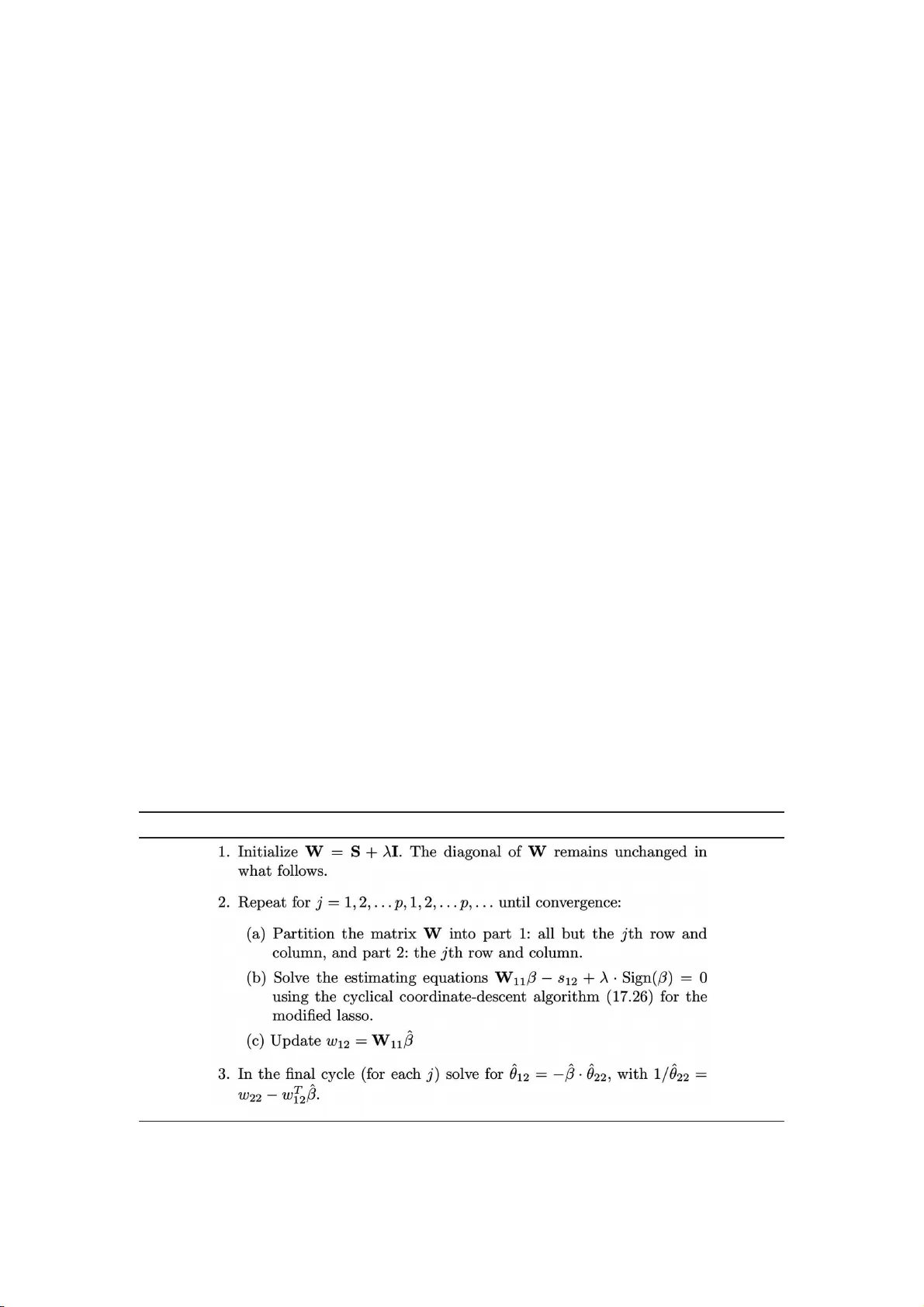
A note on the lac k of symmetry in the graphical lasso Benjamin T. Rolfs a, ∗ , Bala Ra jaratnam b a Inst. for Computational and Appli e d Mathematics, Stanfor d University, Stanfor d, CA 94 395 b Dep artment of Statistics, Stanfor d University, Stanfor d, CA 94305 Abstract The gra phical lasso (g lasso) is a widely-used fast algo rithm for estimating sparse in v erse co v ariance matrices. The glasso solv es an ℓ 1 p enalized maxim um lik eliho o d problem and is a v ailable as an R library on CRAN. The output from the g lasso, a regular ized co v ariance matrix estimate ˆ Σ g lasso and a sparse inv erse co v aria nce matrix estimate ˆ Ω g lasso , not only iden tify a graphical mo del but can also serv e a s in termediate inputs into m ultiv ariate pro cedures suc h as PCA, LDA , MANO V A, and others. The glasso indeed pro duces a co v ariance matrix estimate ˆ Σ g lasso whic h solv es the ℓ 1 p enalized optimization problem in a dual sense; ho w ev er, the metho d for pro ducing ˆ Ω g lasso after this optimization is inexact and ma y pro duce asymmet- ric estimates. This problem is exacerbated when the amoun t of ℓ 1 regularization that is applied is small, whic h in turn is more likely to o ccur if the tr ue underlying in v erse cov ariance matrix is not sparse. The la ck of symmetry can p oten tia lly ha v e consequences. F irst, it implies that ˆ Σ − 1 g lasso 6 = ˆ Ω g lasso and second, asymmetry can p ossibly lead to negativ e or complex eigen v alues, rendering man y m ultiv a riate pro cedures whic h ma y dep end on ˆ Ω g lasso un usable. W e demonstrate this problem, explain its causes, and prop ose p o ssible remedies. Keywor ds: Concen tra t io n mo del selection, g la sso, Graphical Gaussian Mo dels, graphical lasso, ℓ 1 regularization. 1. In tro duction In mo dern applications, man y data sets are simultaneously high- dimensional and lo w in sample size. Classic examples include microarr ay gene express ion and SNP data. D ealing with suc h datasets has b ecome an area of great intere st in man y fields suc h as bio stat istics. Algorithms suc h as the graphical lasso ( F riedman et a l. , 2008 ; Hastie et al. , 2009 ) hav e b een prop osed to obtain regularized cov ariance estimators in the n ≪ p setting ( where n is the sample size and p is the problem dimension) as w ell as p erform gra phical mo del selection. In t he case of the g raphical lasso, graphical mo del selection inv olv es inferring a concen tration graph ( o r equiv alen tly , a Mark ov mo del). A concen tratio n graph enco des zeros in the inv erse co v aria nce (concen tr a tion) matrix, i.e., i 66∼ j for i, j ∈ { 1 , . . . , p } in the graph implies that the partial correlation ρ  X i , X j | X k / ∈{ i,j }  = 0. Along with inferring suc h a graph, the glasso provides p × p dimensional matrix ∗ Corresp o nding author Email addr esses: ben rolfs@ stanf ord.edu (Benjamin T. Rolfs), br ajara t@stan ford.edu (Bala Ra jaratnam) estimators f o r b o th the co v ariance and concen tration matrices, denoted ˆ Σ λ and ˆ Ω λ resp ectiv ely , for a giv en p enalt y parameter λ > 0 . In particular, ˆ Ω λ is the solution to the con v ex maximization problem ˆ Ω λ = ˆ Σ − 1 λ = arg min X ≻ 0 [log det ( X ) − tr ( S X ) − λ k X k 1 ] (1) where S is the sample co v ariance matrix, X = { x ij } p i,j =1 is p ositiv e definite and k X k 1 = P i,j | x ij | . The non-zero elemen ts of ˆ Ω λ corresp ond to edges in the esti- mated concen tra tion gra ph. In some applications, gra phical mo del selection is the primary goa l, where in other situations the estimators ˆ Σ λ and ˆ Ω λ are used as inputs in to other m ultiv ariate algorithms where a regularized co v ariance estimator is required. T ypical examples include LDA, PCA, and MANOV A. Hence, it is often necessary that not only ˆ Σ T λ = ˆ Σ λ ≻ 0, but also that ˆ Ω T λ = ˆ Ω λ , ˆ Ω λ ≻ 0, and ˆ Ω − 1 λ = ˆ Σ λ . W e find that the output of the g r a phical lasso do es not meet these conditions in certain situations, explain wh y , and discuss how to solv e this problem. Such situations ar ise primarily when S is rank-deficien t and λ is small. A lo w lev el of regularization is required when the true underlying concentration matrix is not sparse. It should ho w ev er b e noted that the glasso algorit hm do es indeed solv e the dual pro blem corresp onding to ( 1 ), so the ab o v e assertions should b e interprete d in con t ext. 2. Motiv ating Examples W e now presen t t w o motiv ating examples, one in a classical setting and another in a high-dimensional setting, to illustrate the problem. 2.1. Example 1: L ow dimen sional, lar ge sampl e size inverse c ovarianc e estimation Consider n = 50 0 i . i . d. samples dra wn from a p = 5 dimensional m ultiv aria t e Gaussian distribution with mean µ = 0 and concentration matrix: Ω =       2 . 425 0 . 069 − 0 . 885 0 0 0 . 069 2 . 944 − 0 . 129 0 . 988 0 − 0 . 885 − 0 . 129 2 . 696 0 . 035 − 0 . 974 0 0 . 988 0 . 035 1 . 724 0 . 851 0 0 − 0 . 974 0 . 851 1 . 000       The glasso alg orithm was applied to this da t a set. A regularization parame- ter of λ = 0 . 003 3, whic h is close t o the cross-v alidated estimate, w as c ho sen to demonstrate the problem. The glasso estimators for Ω and Σ = Ω − 1 for a given λ are denoted ˆ Ω λ and ˆ Σ λ . F or reasons whic h are clarified in Section 3 , the gla sso pro duces estimators whic h are neither symmetric nor true in verse s of one another, i.e., ˆ Ω T λ 6 = ˆ Ω λ and ˆ Σ − 1 λ 6 = ˆ Ω λ . T o quan t if y the lack of symmetry , consider the matrix of relativ e errors b et w een the elemen ts of ˆ Ω λ and ˆ Ω T λ , as defined b y E r r ij = 100    ˆ Ω λ ( i,j ) − ˆ Ω T λ ( i,j ) ˆ Ω λ ( i,j )    %. F or the nume rical example ab o v e, E r r =       0 1 . 94 0 . 05 0 0 . 25 1 . 98 0 2 . 84 0 . 04 ∞ 0 . 05 2 . 77 0 0 . 88 0 . 04 0 0 . 04 0 . 89 0 0 . 01 0 . 25 100 . 00 0 . 04 0 . 01 0       2 with t he conv en tion tha t if ˆ Ω λ ( i, j ) = 0 = ˆ Ω λ ( j, i ) then E r r ij = 0. Note that the en tries E r r 5 , 2 = 100% and E r r 2 , 5 = ∞ o ccur b ecause ˆ Ω λ (5 , 2 ) 6 = 0 while ˆ Ω λ (2 , 5 ) = 0. Although the relativ e errors are small, i.e., on the order of 2%, t here is a clear lac k of symmetry in ˆ Ω λ and moreo v er the sparsit y pa tterns in the upp er and lo w er parts of ˆ Ω λ are differen t, and th us yield t w o differen t graphical mo dels. In particular, ˆ Ω λ (5 , 2 ) 6 = 0 whic h indicates an edge b et w een v a r ia bles 2 and 5, while ˆ Ω λ (2 , 5 ) = 0 indicates the absence of suc h. F urthermore, in high-dimensional examples, a graph is often calculated automatically when  ˆ Ω λ  ij > ǫ for some small ǫ . In suc h cases, a lac k of symmetry ma y result, yielding t w o separate graphs. 2.2. Example 2: High dimensional, low samp le size autor e gr e s s ive mo del The lac k of symmetry in ˆ Ω λ , and the resulting difference in the concen tration graphs corresp onding to the upp er a nd low er parts of ˆ Ω λ , often b ecomes more pronounced as the dimension p grow s. W e no w conside r a high dimensional example with n = 250 i.i.d . samples dra wn from a Gaussian AR(1 ) mo del such that X t +1 = φX t + ǫ t for t = 2 , ..., p and X 1 = ǫ 1 . Here, p = 500 , φ = 0 . 75 , and ǫ t i.i.d ∼ N (0 , 1), t = 1 , . . . , p . The concen tra tion mat r ix Ω is tridiagonal, with the diagonal en tries equal to 1 and the off-diagonal en tries equal to − 0 . 75. Giv en a glasso estimator ˆ Ω λ , let E 1 and E 2 denote the edge sets corresp onding to the upp er and low er halv es of ˆ Ω λ , resp ectiv ely . Then the symmetric difference | E 1 ∆ E 2 | is the n um b er of edges whic h are presen t in the concen tration graph enco ded b y one half of ˆ Ω λ but not in the graph enco ded b y the other half. The glasso algorithm was applied to samples from the ab o v e mo del with the regularization parameter λ ta king v alues b et w een 0 . 001 and 0 . 03 in incremen t s of 0 . 001. T o put t hese v alues in p erspectiv e, note that when λ = 0 . 0 3, 102 , 278 out of 124 , 750 (82%) of the estimated off- diagonal en t ries were 0. The num b er of edge differences | E 1 ∆ E 2 | correspo nding to ˆ Ω λ as λ v aries b et w een 0 . 001 a nd 0 . 03 is sho wn in Figure 1 . Figure 1 : | E 1 ∆ E 2 | vs . λ for an AR (1) model with φ = 0 . 75 , p = 50 0 , and n = 250. The r e d dashed line is at | E 1 ∆ E 2 | = 2 0 . Note that at small v alues of λ , the difference in the gra phs corresp onding to the upp er and lo w er parts of ˆ Ω λ as denoted b y | E 1 ∆ E 2 | can b e substantial. Hence, 3 the lac k of symmetry in ˆ Ω λ can result in t w o completely differen t graphical mo d- els. Moreo v er, although | E 1 ∆ E 2 | decreases a s λ increases it nev ertheless remains nonzero as regularization increases. 2.3. Conse quenc es of asymmetry in the glasso c onc entr ation matrix estimator Users o f the glasso ma y find the lac k o f symmetry a problem for a n um b er of reasons: 1. ˆ Ω λ is not a mathematically v alid estimator for ˆ Ω, since ˆ Ω T λ 6 = ˆ Ω λ and ˆ Ω λ 6 = ˆ Σ − 1 λ . 2. There is no guarantee that ˆ Ω λ has real p ositiv e eigenv alues. If it has negativ e or complex eigen v alues, man y m ultiv ariate pro cedures suc h as LDA and PCA ma y not b e w ell-defined. 3. There may b e differences b et w een the edge sets of the concen tr ation graphs corresp onding to the resp ectiv e upp er and low er halves of ˆ Ω λ . W e examine the causes of the lack of symmetry in Section 3 a nd suggest p ossible remedies in Section 4 . 3. Cause of Asymmetry in t he Glasso Concentration Matrix Estimator The glasso algorithm, t ak en directly fro m Hastie et al. ( 2 0 09 ), is sho wn in Algorithm 1 . F or further details concerning t he glasso and its conv ergence, see F riedman et a l. ( 200 8 ) and Hastie et al. ( 2009 ). In Algorithm 1 , S is the sample co v ariance matrix, λ is the gla sso p enalty parameter, a nd W is a matrix o n whic h the g lasso iterates. In Step 2 of Algorithm 1 , W 11 refers to the submatrix of W without its j th ro w and column, and s 12 is the j th column of the sample cov ariance matrix without the diagonal elemen t s j j . In Step 3 of Algorithm 1 , ˆ θ 12 for a giv en j is the j th column of the matrix Θ without Θ j j . Up o n termination o f the algorithm, the current itera t e W is set to ˆ Σ λ and Θ is set to ˆ Ω λ , and referred to as the glasso estimators. Algorithm 1 The glasso, exactly as it app ears on p. 636 of Hastie et al. ( 2009 ). 4 3.1. Construction of ˆ Ω λ in the glasso The glasso iterativ ely up da t es a matrix W whic h con v erges num erically to ˆ Σ λ , the glasso estimator for the p opulation co v a r ia nce mat rix Σ. In con trast, the estimator ˆ Ω λ for t he precision matrix Ω is constructed only up on con v ergence, i.e., only after the algorithm terminates. As w e shall sho w b elo w, the pr o cess by whic h ˆ Ω λ is constructed av oids in v ersion but is ho w ev er mathematically inexact in the sense that it leads to ˆ Ω T λ 6 = ˆ Ω λ and ˆ Ω − 1 λ 6 = ˆ Σ λ . If ˆ Ω T λ 6 = ˆ Ω λ , the gra ph enco ded b y the glasso output ˆ Ω λ ma y b e differen t fro m the graph enco ded b y ˆ Σ − 1 λ . This problem w as illustrated in the tw o mo t iv ating examples ab ov e. Step 2 of Algorithm 1 in v olv es an inner lo op in whic h row/c olumn 1 , . . . , p of W are sequen tially up dated. F or one full inner lo o p ov er the p rows and columns of W , let the p successiv e estimates b e denoted W ( i ) for i = 1 , . . . , p . Exactly one ro w and column of W ( i ) is up dated using a lasso co efficien t ˆ β ( i ) ( ˆ β of Step 2 in Algorithm 1 ). W e no w in tro duce additional notatio n in order to illustrate the problems en- coun tered when the glasso constructs an estimate of the conce ntration matrix (recall that this tak es place up o n termination of the glasso algorithm). Consider once more W ( i ) for i = 1 , . . . , p . Define Θ ( i ) ,  W ( i )  − 1 and θ ( i ) − i,i to b e the ( p − 1 ) v ector consisting of the i th column of Θ ( i ) excluding the diagonal en try θ ( i ) ii . De- fine w ( i ) − i,i and w ( i ) ii b e the cor r esp o nding eleme nts of W ( i ) and let W ( i ) − i, − i b e the i th principal minor of W ( i ) . Then using the fact that Θ ( i ) ,  W ( i )  − 1 , there is a closed-form expression for θ ( i ) ii and θ ( i ) − i,i in terms of s ii , w ( i ) − i,i , and ˆ β ( i ) : θ ( i ) − i,i = − ˆ β ( i ) θ ( i ) ii , θ ( i ) ii = 1 w ( i ) ii −  w ( i ) − i,i  T ˆ β ( i ) . (2) When the glasso terminates, it sets ˆ Σ λ = W ( p ) and uses ( 2 ) to compute n θ ( i ) ii , θ ( i ) − i,i o p i =1 , whic h are taken as the columns of ˆ Ω λ . This pro cedure has a com- plexit y of O ( p 2 ) a nd is therefore more efficien t than direct n umerical in v ersion. 3.2. Cause of asymmetry in ˆ Ω λ The glasso terminates when W conv erges n umerically , a nd constructs ˆ Ω λ from n θ ( i ) − i,i , θ ( i ) ii o p i =1 . These are easily obtainable from previous iteratio ns of the inner lo op, thus av oiding the need to inv ert W ( p ) . Ho we v er, while n θ ( p ) − p,p , θ ( p ) pp o is equal to the the p t h row a nd column of Θ ( p ) =  W ( p )  − 1 , ˆ Σ − 1 λ b y construction, the n θ ( i ) ii , θ ( i ) i, − i o p − 1 i =1 are not equal to the i th ro w and column of  W ( p )  − 1 . Instead, b y construction eac h n θ ( i ) ii , θ ( i ) i, − i o p − 1 i =1 is equal to the i th ro w and column of  W ( i )  − 1 6 =  W ( p )  − 1 . Asymmetry o ccurs b ecause the quan tities n θ ( i ) ii , θ ( i ) i, − i o p i =1 are taken as the columns of ˆ Ω λ . The discrepancy b et w een the ab o v e set of estimates may not b e minimal ev en if the iterates W ( i ) are approxim ately equal. Another wa y of stating this problem is that conv ergence of the W ( i ) to a sp ecified tolerance do es not necessarily imply 5 con v ergence o f  W ( i )  − 1 to an y g iv en tolerance. The result is tha t while the glasso co v ariance estimator ˆ Σ λ satisfies ( 1 ), ˆ Ω λ do es not, leading to the aforemen tioned problems. The pro blem is exacerbated when the p enalty parameter λ is small and S is close to ra nk-deficien t (whic h is the case when n ≪ p ). The follow ing lemma formalizes this assertion. Lemma 1. If S is r an k-deficient, the maxim um absolute value of the entries of ˆ Ω λ diver ges as λ → 0 . Pr o of. See the app endix. Lemma ( 1 ) sugg ests that conv ergence of t he inv erse glasso iterates W − 1 to some small, fixed tolerance ma y require a radically small to lerance criterion for the conv ergence of the glasso iterates W . Indee d, it is easy to construc t suc h examples. Consider the rank-deficien t sample co v ariance matrix S shown b elo w alongside the optimal solution to ( 1 ) corresp onding to a regularization parameter of λ = 10 − 6 : S =  1 0 0 0  , ˆ Σ λ =  1 + 10 − 6 0 0 10 − 6  , ˆ Ω λ =  (1 + 1 0 − 6 ) − 1 0 0 10 6  . (3) Moreo v er, consider a matrix iterate W t whic h is close to ˆ Σ λ , giv en as follow s W t =  1 + 10 − 6 0 0 (1 + t − 1 ) × 1 0 − 6  . (4) The suprem um-norm errors on the dua l and primal for this W t are giv en resp ec- tiv ely b y    W t − ˆ Σ λ    ∞ = t − 1 10 − 6 and    W − 1 t − ˆ Ω λ    ∞ = 1 t + 1 10 6 , (5) and are sev eral orders of magnitude a pa rt. This example demonstrates wh y de- creasing the con v ergence tolerance on the dual iterates W ma y not a lw a ys b e a feasible solution to the asymmetry problem discussed here. T o summarize, the metho d for in v ersion used during the final step of t he g la sso algorithm for computing ˆ Ω λ is mathematically inexact, and the resulting error is exacerbated whe n p > n with an insuffic ien tly large p enalt y parameter λ . In this case, the ℓ 1 -p enalized in vers e cov ariance estimator is unreliable as λ → 0, a s described by Lemma 1 Therefore the use of an o v erly small λ should b e a v oided; ho w ev er, in pr a ctice, choosing the p enalt y parameter λ can b e c hallenging. F or example, choosing λ via cross-v alidation using ˆ Ω λ tends to yield ov erly small λ , whic h may pro duce dense and p ossibly ill-conditioned estimates for ˆ Ω λ . One p ossible indicator of to o little r egula rization is when the n um b er of neigh b ors of eac h v ariable/no de is to o high. A second p ossible indicator is if there is a serious lac k of symmetry in the glasso estimates. A third p ossible indicator is when the condition n um b er of the resulting estimate is to o hig h. Recen tly , W on et al. ( 20 1 2 ) pro vide imp etus for constraining the condition n um b er of the cov ariance matrix; in ligh t o f that w ork, the condition n um b er can p erhaps b e used a s a guide in c ho osing λ . 6 4. Enforcing Symmetry on the Glasso C o ncentration Matrix Estimator The glasso co v ariance estimator ˆ Σ λ is the true n umeric minim um of the glasso problem ( 1 ) and thu s a v alid ℓ 1 regularized estimator for the true p opulation co v ariance matrix Σ. Ho w ev er, as previously demonstrated, the gla sso estimator ˆ Ω λ is asymmetric, and ˆ Ω − 1 λ 6 = ˆ Σ λ . In some settings, it ma y b e desirable to resolv e one or b oth of the af o remen- tioned issues. F or ˆ Ω λ to enco de a sparse concen tratio n gra ph, its sparsit y pat t ern m ust b e symme tric. Moreo ver, if ˆ Ω λ is to b e used as a sparse concen tration ma- trix estimator, it is necess ary that ˆ Ω T λ = ˆ Ω λ for it to b e a v a lid estimator. M ost imp ortantly , it may b e required that ˆ Ω λ = ˆ Σ − 1 λ ≻ 0 in order f o r it to b e usable in m ultiv ariate pro cedure s. W e prop ose three simple approaches which address some or all of the ab ov e requiremen ts. 1. Numerical in v ersion. T o hav e ˆ Ω λ = ˆ Σ − 1 λ , it is necessary to directly in v ert ˆ Σ λ . This inv ersion main tains the sparsit y pattern of ˆ Ω λ (although as a consequence o f numeric al error there may b e negligible entries in place of zero es). Th e O ( p 3 ) complexit y of n umerical inv ersion (vs. O ( p 2 ) for the current glasso approac h) do es not represen t a difficult y for matr ices of the dimension whic h the glasso is curren tly able to solve ( up to p ≈ 2000 on a ty pical des ktop), as it also needs to b e done only o nce at the end of the glasso iteration. Note that the inv erted matrix ˆ Σ − 1 λ should b e hard thresholded to eliminate small no n-zero en tries introduced b y n umerical error, and the resulting inv erse co v ariance matrix then should b e chec k ed for p ositiv e definiteness. Ho w ev er, numerical in v ersion ma y not b e a viable option when ˆ Σ λ is ill- conditioned, as is t he case when S is ra nk-deficien t and λ is small. In suc h cases, it may b e useful to exercise caution when using ˆ Ω λ in further calculations. 2. Mo dified glasso output. The upp er right triangle of ˆ Ω λ can b e tak en as the corr ect estimate. The en tries correspo nding to the upp er right triangle are more recen t up dat es than those in the low er left triangle, since the glasso inserts the n θ ( i ) − i,i , θ ( i ) ii o p i =1 in to the columns of ˆ Ω λ . The resulting estimator will not equal ˆ Σ − 1 λ , but it is symmetric. It will not solv e the primal problem in ( 1 ) exactly . 3. Iterativ e prop ort ional fitting (I PF) . IPF ( Sp eed and Kiiv eri , 19 86 ) can b e used to sim ultaneously compute the maxim um lik eliho o d estimates for Ω and Σ under an assumed concen tratio n graph, i.e., sparsit y pattern in ˆ Ω. One approach is t o use the sparsit y pattern from the upp er rig ht triangle of ˆ Ω λ , enforce symmetry , and then use IPF to obtain ˆ Σ and ˆ Ω. The esti- mator ˆ Ω will reflect the sparsity structure corresp onding to ˆ Ω λ , and satisfy ˆ Ω = ˆ Σ − 1 at each iteration of IPF. Note that neither ˆ Ω nor ˆ Σ will b e solu- tions to ( 1 ) or ( 6 ), resp ectiv ely . F urthermore, the computational complexit y of IPF is O ( c 3 ), where c is the size of the largest maximal clique of the graph implied by ˆ Ω λ . Therefore, IPF do es not imply relativ ely higher computa- tional costs, althoug h it do es require iden tifying the maximal cliques whic h is w ell-known to b e NP-complete. Finding the maximal cliques can how ev er b e av oided if a mo dification of the glasso algorithm is used to estimate an 7 undirected Gaussian graphical mo del with kno wn structure (see Algorithm 17.1 in Hastie et al. ( 2009 )). T able 1 summarizes the prop erties and tradeoffs of eac h of the prop osed solu- tions. T able 1: Comparis o n of p ossible estimators. Metho d ˆ Ω T = ˆ Ω Latest up dates in ˆ Ω ˆ Ω = ˆ Σ − 1 ˆ Σ solv es ( 6 ) ˆ Ω solv es ( 1 ) Glasso Output X X X X X Mo dified Output X X X X X Numerical In v ersion X X X X X IPF X X X X X 5. Conclusions In this note we demonstrated that the estimators from the widely used R pac k age glasso ma y b e asymmetric when the amoun t of regularization applied is small. This could cause problems when the glasso estimators are used as inputs to ot her m ultiv ariate pro cedures, and additionally b ecause the sparsit y structure of the glasso estimators may themselv es b e asymmetric. It may b e helpful f or users of the pac k age glas so to b e a w are of this, as the estimator can b e easily corrected by one of the outlined metho ds. Of these, n umerical in v ersion follo w ed b y thresholding ma y b e the simplest and most effectiv e fix. Th e ro ot cause of the issue is that the glasso alg o rithm op erates o n the dual of ( 1 ), and constructs the primal estimator, ˆ Ω λ , only after t he dual optimization completes. If a sparse concen tra tion estimator is sough t, it may b e more natural t o op erate off the primal problem ( 1 ), though the glasso is more p opular in practice. Me tho ds fo r solving the primal ( 1 ) hav e b een recently considered, among o thers see Maleki et al. ( 2 0 10 ) and Mazumder and Agarw al ( 2 011 ). This short note av oids recourse to the primal b y iden tifying problems with the dual approach, and consequen tly explores w ays in whic h these can b e easily rectified so that the p opular dual approac h can b e retained. Ac kno wledgmen ts W e ac kno wledge T rev or Hastie and Rob ert Tibshirani (Depart ment of Stat is- tics, Stanford Univ ersit y) for discussions. Benjamin Rolfs was supp ort ed in par t b y the Depart ment of Energy Office of Science Graduate F ello wship Prog r a m DE-A C05-06OR 23100 (ARR A) and NSF gran t A GS10038 23. Bala Ra jaratna m w as supp orted in part b y NSF gran ts DMS0906392 (ARRA), A GS10 0 3823, DMS (CMG) 102 5465, DMS1106 6 42 and gran ts NSA H98230- 11-1-0 194, D ARP A-YF A N66001-11- 1-4131 and SUFSC10- SUSHSTF09-SMSCVISG0906. References Banerjee, O ., E l Ghaoui, L., d’Aspremont, A., 2008. Mo del selection thr o ugh spar se maximum likelihoo d estimation for mu ltiv a rate g aussian or binary data. Journal of Machine Lear ning Research 9, 48 5 –516 . 8 F riedman, J., Hastie, T., Tibshirani, R., 200 8 . Sparse in verse cov ariance estimatio n with the graphical lasso . Biostatistics 9, 432– 441. Hastie, T., Tibshirani, R., F r iedman, J ., 200 9. E le men ts of Statistical Lear ning. Spr inger, New Y ork. 2nd e ditio n. Maleki, A., Ra jaratnam, B., W ong, I., 201 0. F ast iter ative thresholding algor ithms for sparse inv er se cov ar iance Selection. T ec hnical Rep ort. Mazumder, R., Agarwal, D.K., 2 011. A flexible, scalable and efficient alg orithmic fra mework fo r the Primal gra phical la sso. Pr e-print arXiv: 1110. 5508v1 . Spee d, T., Kiiveri, H., 19 86. Ga ussian marko v distributions over finite graphs. Annals of Statistics 14, 138 –150. W on, J., Lim, J., K im, S., Ra jaratna m, B., 2012 . Condition num b er regular ized cov ariance estimation. Jour nal o f the Roy al Statistical So ciety Series B (in press) . App endix Pr o of. Consider the dual of ( 1 ) as giv en in Banerjee et al. ( 2008 ): ˆ Σ λ = arg min X ≻ 0 [log det ( X )] (6) s.t. max i,j | x ij − s ij | ≤ λ where max i,j | m ij | is the suprem um norm, the maxim um absolute v alue en t r y of the matrix M . F rom ( 6 ), it is clear that ˆ Σ λ → S in t he suprem um norm as λ → 0, though at λ = 0 the primal problem ( 1 ) do es not nece ssarily ha v e a solution. Con v ergence in sup-norm gives con v ergence of ˆ Σ λ → S in an y other op erator norm k•k ⋆ . In par ticular, inv oking the contin uity of eigen v a lues, λ min  ˆ Σ λ  → λ min ( S ) as λ → 0, with λ min ( M ) defined as the smallest eigenv alue of the square matr ix M . Conside ring the o p erator 2-norm and ∞ -no r m of ˆ Σ − 1 λ giv es: max i,j      ˆ Ω λ  ij     = max i,j      ˆ Σ − 1 λ  ij     ≥ p − 1    ˆ Σ − 1 λ    ∞ ≥ p − 1    ˆ Σ − 1 λ    2 = p − 1 λ max  ˆ Σ − 1 λ  = p − 1 h λ min  ˆ Σ λ i − 1 − → λ → 0 p − 1 [ λ min ( S )] − 1 In the sample-deficien t case n ≪ p , λ min ( S ) = 0 almost surely , and therefore ˆ Ω λ div erg es with resp ect to the suprem um norm as λ → 0. 9