Expectation-Propagation for Likelihood-Free Inference

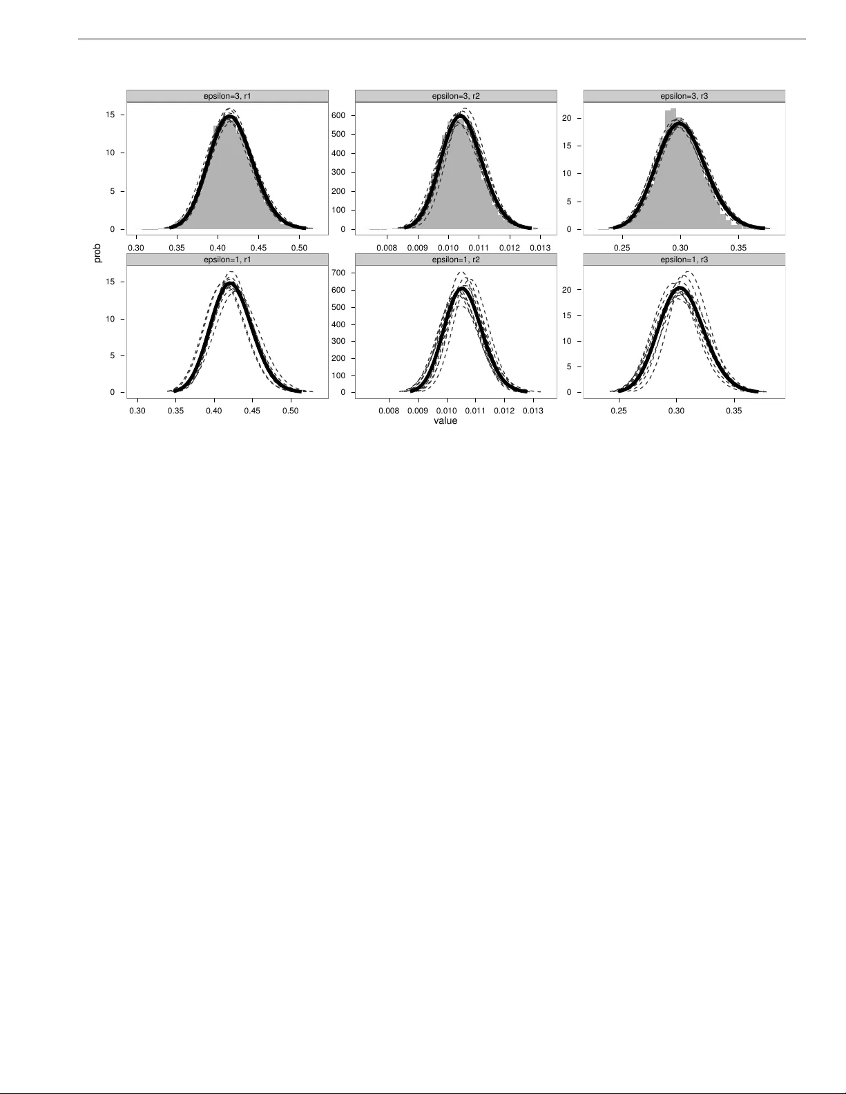
Exp ectation-Propagation fo r Lik eliho o d-F ree Inference Simon Ba rthelmé ∗ Nicolas Chopin † Abstract Man y mo dels of in terest in the natural and so cial sciences hav e no closed-form likelihoo d function, which means that they cannot b e treated using the usual techniques of statistical inference. In the case where such mo dels can b e efficien tly simulated, Bay esian inference is still p ossible thanks to the Approximate Bay esian Computation (ABC) algorithm. Although man y refinemen ts ha v e b een suggested, ABC inference is still far from routine. ABC is often excruciatingly slow due to very low acceptance rates. In addition, ABC requires introducing a v ector of “summary statistics” s ( y ) , the choice of whic h is relatively arbitrary , and often require some trial and error, making the whole process quite lab orious for the user. W e introduce in this work the EP-ABC algorithm, whic h is an adaptation to the lik elihoo d-free con text of the v ariational appro ximation algorithm known as Expectation Propagation (Mink a, 2001a). The main adv antage of EP-ABC is that it is faster by a few orders of magnitude than standard algorithms, while pro ducing an ov erall approximation error which is typically negligible. A second adv an tage of EP-ABC is that it replaces the usual global ABC constraint k s ( y ) − s ( y ? ) k ≤ ε , where s ( y ? ) is the vector of summary statistics computed on the whole dataset, b y n lo cal constrain ts of the form k s i ( y i ) − s i ( y ? i ) k ≤ ε that apply separately to eac h data-point. In particular, it is often possible to take s i ( y i ) = y i , making it p ossible to do a wa y with summary statistics en tirely . In that case, EP-ABC makes it possible to approximate directly the evidence (marginal likelihoo d) of the mo del. Comparisons are p erformed in three real-world applications whic h are typical of lik elihoo d-free inference, including one applic- ation in neuroscience which is no v el, and p ossibly too challenging for standard ABC techniques. Key-w ords: Approximate Bay esian Computation; Comp osite Lik elihoo d; Exp ectation Propagation; Likelihoo d-F ree Inference; Quasi-Mon te Carlo. 1 Intro duction In natural and so cial sciences, one finds many examples of probabilistic mo dels whose likelihoo d function is intractable. This includes most mo dels of noisy biological neural netw orks (Gerstner and Kistler, 2002), some time series and choice mo dels in Economics (T rain, 2003), phylogenetic models in evolutionary Biology (Beaumont, 2010), spatial extremes in En vironmen tal Statistics (Da vison et al., 2012), among others. That the lik eliho o d is intractable is unfortunate, b ecause one would still lik e to p erform the usual statistical tasks of parameter i nference and mo del comparison, and the traditional statistical to ol-kit assumes that the lik elihoo d function is either directly a v ailable or can b e made so b y in tro ducing laten t v ariables. This explains that researchers hav e often had to con tent themselves with semi-quantitativ e analyses sho wing that a mo del could repro duce some asp ect of an empirical phenomenon for some v alues of the parameters; for t w o represen tativ e examples from vision science, see Nuthmann et al. (2010), Brascamp et al. (2006). A breakthrough was pro vided by the work of T a v aré et al. (1997), Pritchard et al. (1999) and Beaumont et al. (2002), in the form of the Approximate Ba y esian Computation (ABC) algorithm, which enables Bay esian inference in the likelihoo d- free context. (See also Diggle and Gratton (1984) and Rubin (1984) for early versions of ABC.) Assuming some mo del p ( y ∗ | θ ) for the data y ? , and a prior p ( θ ) o v er the parameter θ ∈ Θ , the ABC algorithm iterates the following steps: 1. Dra w θ from the prior, θ ∼ p ( θ ) . 2. Dra w a dataset y from the mo del conditional on θ , y | θ ∼ p ( y | θ ) . 3. If d ( y , y ∗ ) ≤  , then keep θ , otherwise reject. and therefore pro duces samples from the so-called ABC posterior: ∗ Université de Genèv e. F aculté de Psyc hologie et de Sciences de l’Education, Unimail CH-1211 Genèv e 4, Switzerland. si- mon.barthelme@unige.ch † CREST/ENSAE. 3, A v enue Pierre Larousse 92245 Malakoff CEDEX F rance. nicolas.chopin@ensae.fr 1 1 Intro duction 2 p  ( θ | y ∗ ) ∝ p ( θ ) ˆ p ( y | θ ) 1 { d ( y , y ? ) ≤  } d y . (1.1) The pseudo-distance is usually taken to b e d ( y , y ? ) = || s ( y ) − s ( y ∗ ) || , for some norm || · || , where s ( y ) is a vector of summary statistics, for example some empirical quantiles or momen ts of y . Unless s is sufficient, the approximation error do es not v anish as  → 0 , as p ( θ | s ( y ? )) 6 = p ( θ | y ? ) . In that resp ect, the ABC p osterior suffers from tw o levels of appro ximation: a nonparametric error, akin to the error of kernel density estimation, and where  pla ys the role of a bandwidth (see e.g. Blum, 2010), and a bias introduced by the summary statistics s . The more we include in s ( y ) , the smaller the bias induced b y s should b e. On the other hand, as the dimensionality of s ( y ) increases, the low er the acceptance rate will b e. W e would then ha ve to increase  , which leads to an approximation of low er quality . Th us, ABC requires in practice some more or less arbitrary compromise b etw een what summary statistics to include and how to set . T o establish that the results of the inference are somewhat robust to these c hoices, many runs of the algorithm may be required. Although several v ariants of the original ABC algorithm that aim at increasing acceptance rates exist (e.g. Beaumon t et al., 2002), the current state of the matter is that an ABC analysis is very far from routine use b ecause it may take days to tune on real problems. The semi-automatic metho d for constructing summary statistics recen tly prop osed by F earnhead and Prangle (2012) seems to alleviate partly these problems, but it still requires at least one, and sometimes several pilot runs. In this article we in troduce EP-ABC, an adaptation of the Exp ectation Propagation (EP) algorithm (Mink a, 2001a; Bishop, 2006, Chap. 10) to the likelihoo d-free setting. The main adv antage of EP-ABC is that it is muc h faster than previous ABC algorithms: typically , it provides accurate results in a few minutes, whereas a standard ABC algorithm may need sev eral hours, or even days. EP-ABC requires that the data y ? ma y b e decomp osed into n “c hunks”, y ? 1 , . . . , y ? n (of p ossibly different dimensionality or supp ort), in such a wa y that is p ossible to simulate sequentially the n ch unks; i.e. one is able to simulate from p ( y ? i | y ? 1: i − 1 , θ ) for each i . More precisely , EP-ABC builds an EP appro ximation of the following t yp e of ABC p osterior distributions: p  ( θ | y ? ) ∝ p ( θ ) n Y i =1  ˆ p ( y i | y ? 1: i − 1 , θ ) 1 { k s i ( y i ) − s i ( y ? i ) k≤ ε } dy i  (1.2) where s i ( y i ) is a summary statistic sp ecific to ch unk i , and with the conv ention that p ( y 1 | y ? 1:0 , θ ) = p ( y 1 | θ ) . Giv en the w a y it op erates, we shall see that EP-ABC essen tially replaces the initial, p ossibly difficult ABC problem, by n ABC simpler (i.e. lo w er-dimensional) ABC problems. In particular, it ma y b e easier to construct a set of “lo cal” summary statistics s i ( y i ) for each c h unk y i rather than a global set s ( y ) the whole dataset y , in such a w a y that the probability that k s i ( y i ) − s i ( y ? i ) k ≤ ε is not too small. Of course, not all ABC mo dels are amenable to the factorisation in (1.2), at least directly . W e shall discuss this p oint more in detail in the paper. A t the very least, factorisable models include situations with n rep eated exp eriments, which are not easily tackled through standard ABC, b ecause of the difficult y to define some vector s ( y ) which summarises these n exp eriments. Bazin et al. (2010) discusses this p oin t, in the context of genetic data collected ov er a large num b er of lo ci, and recommend instead to construct lo ci-sp ecific summary statistics, and com bine results from lo ci-sp ecific ABC exercises. In certain problems such that y i is of low dimension, it may b e even p ossible to take s i ( y i ) = y i . In that case, EP-ABC pro vides an EP approximation of a summary-less ABC p osterior; that is, when  → 0 (under appropriate measure-theoretic conditions), p  ( θ | y ? ) → p ( θ | y ? ) , the true p osterior. In suc h situations, EP-ABC also provides an approximation of the evidence p ( y ? ) , whic h is a very useful quantit y for mo del comparison. Dean et al. (2011) show that, in the sp ecific con text of hidden Marko v mo dels such that the observ ation density is intractable (as this work was motiv ated by the filtering ABC algorithm dev elop ed in Jasra et al. (2010)), the ABC error of a summary-less ABC algorithm should not b e interpreted as a non-parametric error, but rather as a missp ecification error, where the missp ecified mo del is the true mo del, but with observ ations corrupted with noise. This missp ecification implies a bias of order ε . Thus, in addition to being more con v enien t for the user, as it av oids sp ecifying some summary statistics, summary-less ABC do es not seem to suffer from the curse of dimensionality (in the dimension of s ( y ) ) of standard ABC. Allowing summary-less ABC inference in certain cases seems to b e another adv an tage of EP-ABC. W e start with a generic description of the EP algorithm, in Section 2, and explain in Section 3 ho w it can b e adapted to the lik eliho o d-free setting. W e explain in Section 4 how EP-ABC can b e made particularly efficien t when data-p oints are I ID (indep endent and iden tically distributed). Section 5 contains three case studies drawn from finance, p opulation ecology , and vision science. The t wo first examples are b orrow ed from already known applications of ABC, and illustrate to which extent EP-ABC ma y outp erform standard ABC techniques in realistic scenarios. T o the b est of our knowledge, our third example from vision science is a nov el application of likelihoo d-free inference, which, as whic h shall argue, seems to o challenging for standard ABC techniques. 2 Exp ectation Propagation 3 Section 6 discusses ho w EP-ABC may cop e with difficult posteriors through tw o additional examples. Section 7 discusses p ossible extensions of EP-ABC; in particular, for non-factorisable likelihoo ds. In such cases, one may replace the likelihoo d by some factorisable approximation, suc h as a comp osite likelihoo d. Section 8 concludes. W e use the following notations throughout the pap er: b old letters refer to vectors or matrices, e.g. θ , λ , Σ and so on. W e also use b old face to distinguish complete sets of observ ations, i.e. y or y ? , from their comp onen ts, y i , and y ? i , i = 1 , . . . n , although w e do not assume that these comp onents are necessarily scalar. F or sub-vectors of observ ations, we use the colon notation: y 1: i = ( y 1 , . . . , y i ) . The notation k · k refers to a generic norm, and k · k 2 refers to the Euclidean norm. The Kullbac k-Leibler divergence b et w een probabilit y densities π and q is denoted as K L ( π k q ) = ˆ π ( θ ) log  π ( θ ) q ( θ )  d θ . The letter p alw a ys refers to probability densities concerning the mo del; i.e. p ( θ ) is the prior, p ( y 1 | θ ) is the likelihoo d of the first observ ation, and so on. T ransp ose of a matrix A is denoted A t , and the diagonal matrix with diagonal elements giv en b y vector V is diag( V ) . 2 Exp ectation Propagation Exp ectation Propagation (EP , Mink a, 2001a) is an algorithm for v ariational inference, a class of tec hniques that aim at finding a tractable probability distribution q ( θ ) that b est approximates an intractable target densit y π ( θ ) . One wa y to form ulate this goal is as fi nding the member of some parametric family Q that is in some sense closest to π ( θ ) , where “closest” is defined by some divergence b etw een probabilit y distributions. A distinctiv e feature of EP is that it based on the divergence K L ( π || q ) , whereas man y v ariational methods (e.g. V ariational Bay es, see Chap. 10 of Bishop, 2006) try to minimize K L ( q || π ) . F or a go o d discussion of the relativ e merits of each divergence, see Bishop (2006, p. 468-470) and Mink a (2005). As a brief summary , minimizing K L ( q || π ) tends to pro duce appro ximation that are too compact; see also W ang and Titterington (2005). The divergence K L ( π || q ) do es not suffer from this drawbac k, and is p erhaps more app ealing from a statistical p oint of view (if only because maximum lik elihoo d estimation is based on the corresponding con trast), but on the other hand, minimizing K L ( π || q ) when π is multimodal tends to pro duce an appro ximation that co v ers all the mo des, and therefore has to o large a supp ort. W e shall return to this p oin t. 2.1 Assumptions of Exp ectation Propagation EP assumes that the target density π ( θ ) decomp oses in to a pro duct of simpler factors π ( θ ) = 1 Z π n Y i =0 l i ( θ ) (2.1) and exploits this factorisation in order to construct a sequence of simpler problems. F or instance, l 0 ( θ ) may b e the prior p ( θ ) , l i ( θ ) = p ( y i | y 1: i − 1 , θ ) if y is a set of n observ ations y i , with the conv ention that p ( y 1 | y 1:0 , θ ) = p ( y 1 | θ ) , and Z π = p ( y ) . EP uses an approximating distribution with a similar structure: q ( θ ) ∝ n Y i =0 f i ( θ ) (2.2) where the f i ’s are known as the “sites”. In a spirit close to a co ordinate-descent optimization algorithm, eac h site is up dated in turn, while the n other sites are k ept fixed. F or the sake of conciseness, w e focus in this pap er on Gaussian sites, expressed under their natural parametrisation: f i ( θ ) = exp  − 1 2 θ t Q i θ + r t i θ  , where Q i and r i are called from no w on the site p ar ameters. This generates the follo wing Gaussian approximation q : q ( θ ) ∝ exp    − 1 2 θ t n X i =0 Q i ! θ + n X i =0 r i ! t θ    . (2.3) In addition, we assume that the true prior p ( θ ) is Gaussian, with natural parameters Q 0 and r 0 . In that case, the site f 0 is kept equal to the prior, and only the sites f 1 to f n are up dated. W e note ho w ev er that EP may easily accommo date a non-Gaussian prior (b y simply treating the prior as additional factor to be appro ximated), or other types of parametric sites. In fact, the site up date described in the following section ma y b e easily adapted to any exp onential family; see Seeger (2005). 2 Exp ectation Propagation 4 2.2 Site up date Supp ose that (2.2) is the current appro ximation, and one wishes to up date site i . This is done by creating a “hybrid” distribution, obtained by substituting site i with the true likelihoo d contribution l i ( θ ) : h ( θ ) ∝ q − i ( θ ) l i ( θ ) , q − i ( θ ) = Y j 6 = i f j ( θ ) . (2.4) F or Gaussian sites, this leads to: h ( θ ) ∝ l i ( θ ) exp  − 1 2 θ t Q − i θ + r t − i θ  , Q − i = X j 6 = i Q j , r − i = X j 6 = i r j . The new v alue of site f i is then obtained by minimising with respect to f i the Kullbac k-Leibler pseudo-distance K L ( h i || q ) b etw een the hybrid and the Gaussian approximation q (again keeping the f j ’s fixed). When Gaussian sites are used, this minimisation is equiv alent to taking q to b e the Gaussian densit y with moment parameters that match those of the hybrid distribution Z h = ˆ q − i ( θ ) l i ( θ ) d θ , µ h = 1 Z h ˆ θ q − i ( θ ) l i ( θ ) d θ , Σ h = 1 Z h ˆ θ θ t q − i ( θ ) l i ( θ ) d θ − µ h µ t h . (2.5) A key observ ation at this stage is that the feasibility of EP is essentially dictated b y ho w easily the moments ab ov e ma y be computed. These moments may b e in terpreted as the moments of a p osterior distribution, based on a Gaussian prior, with natural parameters Q − i and r − i , and a likelihoo d consisting of a single factor l i ( θ ) . Finally , from these moment parameters, one may recov er the natural parameters of q , and deduce the new site para- meters for f i as follows: Q i ← Σ − 1 h − Q − i , r i ← Σ − 1 h µ h − r − i . EP pro ceeds b y lo oping ov er sites, up dating each one in turn until conv ergence is achiev ed. In well-behav ed cases, one observes empirically that a small num b er of complete sweeps through the sites is sufficient to obtain conv ergence. Ho w ev er, there is curren tly no general theory on the con vergence of EP . App endix A gives an algorithmic description of EP , in the more general case where an exp onential family is used for the sites. 2.3 App roximation of the evidence EP also provides an approximation of the normalising constant Z π of (2.1), using the same ideas of up dating site appro x- imations through moment matching. T o that effect, we rewrite the EP approximation with normalising constants for each site (assuming again the prior is Gaussian and do es not need to b e appro ximated): q ( θ ) = p ( θ ) n Y i =1 f i ( θ ) C i , f i ( θ ) = exp  − 1 2 θ t Q i θ + r t i θ  . (2.6) Then the up date of site i pro ceeds as b efore, by adjusting C i , r i and Q i through moment matc hing. Simple calculations (see e.g. Seeger, 2005) lead to the follo wing expressions for the up date of C i : log ( C i ) = log ( Z h ) − Ψ( r , Q ) + Ψ( r − i , Q − i ) (2.7) where Z h is the normalising constant of the hybrid, as defined in (2.5), r , Q (resp. r − i , Q − i ) are the natural parameters of the current Gaussian approximation q (resp. of q /f i ∝ Q j 6 = i f j ) and Ψ( r , Q ) is the log-normalising constant of an unnormalised Gaussian density: Ψ( r , Q ) = log  ˆ exp  − 1 2 θ t Qθ + r t θ  d θ  = − 1 2 log | Q / 2 π | + 1 2 r t Qr . 3 EP-ABC: Adapting EP to lik elihoo d-free settings 5 F or each site up date, one calculates C i as defined in (2.7). Then, at the end of the algorithm, one may return the following quan tit y n X i =1 log ( C i ) + Ψ( r , Q ) − Ψ( r 0 , Q 0 ) as an approximation to the logarithm of the evidence. 3 EP-ABC: A dapting EP to likelihoo d-free settings 3.1 Basic p rinciple As explained in the introduction, our ob jective is to approximate the following ABC p osterior p  ( θ | y ? ) ∝ p ( θ ) n Y i =1  ˆ p ( y i | y ? 1: i − 1 , θ ) 1 { k s i ( y i ) − s i ( y ? i ) k≤ ε } dy i  (3.1) whic h corresp onds to a particular factorisation of the lik elihoo d, p ( y ? | θ ) = n Y i =1 p ( y ? i | y ? 1: i − 1 , θ ) . (3.2) Note that, in full generality , the y ? i ma y b e any t ype of “ch unk” of the observ ation vector y ? , i.e. the random v ariables y ? i ma y hav e a different dimension, or more generally different supports. F or simplicit y , we assume that the prior p ( θ ) is Gaussian, with natural parameters Q 0 and r 0 . One ma y in terpret (3.1) as an artificial p osterior distribution, which decomposes into a prior times n likelihoo d con tributions l i , as in (2.1), with l i ( θ ) =  ˆ p ( y i | y ? 1: i − 1 , θ ) 1 { k s i ( y i ) − s i ( y ? i ) k≤ ε } dy i  . W e hav e seen that the feasibility of the EP algorithm is determined by the tractability of the following op eration: to compute the tw o first moments of a pseudo-p osterior, made of a Gaussian prior N d ( µ − i , Σ − i ) , times a single lik eliho o d con tribution l i ( θ ) . This immediately suggests the follo wing EP-ABC algorithm. W e use the EP algorithm, as described in Algorithm 3, and where the moments of such a pseudo-p osterior are computed using as describ ed in Algorithm 1, that is, as Monte Carlo estimates, based on simulated pairs ( θ [ m ] , y [ m ] i ) , where θ [ m ] ∼ N d ( µ − i , Σ − i ) , and y [ m ] i | θ [ m ] ∼ p ( y i | y ? 1: i − 1 , θ [ m ] ) . Algorithm 1 Computing the moments of the h ybrid distribution in the likelihoo d-free setting, basic algorithm. Inputs:  , y ? , i , and the moment parameters µ − i , Σ − i of the Gaussian pseudo-prior q − i . 1. Dra w M v ariates θ [ m ] from a N ( µ − i , Σ − i ) distribution. 2. F or each θ [ m ] , draw y [ m ] i ∼ p ( y i | y ? 1: i − 1 , θ [ m ] ) . 3. Compute the empirical moments M acc = M X m =1 1 n k s i ( y [ m ] i ) − s i ( y ? i ) k≤ ε o , b µ h = P M m =1 θ [ m ] 1 n k s i ( y [ m ] i ) − s i ( y ? i ) k≤ ε o M acc (3.3) b Σ h = P M m =1 θ [ m ]  θ [ m ]  t 1 n k s i ( y [ m ] i ) − s i ( y ? i ) k≤ ε o M acc − b µ h b µ t h . (3.4) Return b Z h = M acc / M , b µ h and b Σ h . Since EP-ABC in tegrates one data-p oint at a time, it do es not suffer from a curse of dimensionality with resp ect to n : the rejection rate of Algorithm 1 corresp onds to a single constraint k s i ( y i ) − s i ( y ? i ) k ≤  , not n of them, and is therefore 3 EP-ABC: Adapting EP to lik elihoo d-free settings 6 lik ely to b e tolerably small even for small windows  . (Otherwise, in v ery challenging situations, one has the lib erty to replace Algorithm 1 by a more elaborate ABC algorithm.) The only requirement of EP-ABC is that the factorisation of the lik eliho o d, (3.2), is c hosen in suc h a wa y that sim ulating from the model, i.e. y ∼ p ( y | θ ) can b e decomp osed into a sequence of steps, where one samples from p ( y i | y 1: i − 1 , θ ) , for i = 1 , . . . , n . W e shall see in our examples section, see Section 5, that several imp ortant applications of lik eliho o d-free inference fulfil this requiremen t. W e shall also discuss in Section 7 ho w other likelihoo d-free situations ma y b e accommo dated by the EP-ABC approac h. 3.2 Numerical stabilit y EP-ABC is a sto chastic version of EP , a deterministic algorithm, hence some care must b e taken to ensure n umerical stabilit y . W e describ e here three strategies to wards this aim. First, to ensure that the sto chastic error introduced by each site up date do es not v ary to o m uch in the course of the algorithm, w e adapt dynamically M , the num b er of sim ulated points, as follo ws. F or a given site up date, w e sample rep etitiv ely M 0 pairs ( θ [ m ] , y [ m ] i ) , as describ ed in Algorithm 1, until the total n um ber of accepted p oints exceeds some threshold M min . Then w e compute the moments (3.3) and (3.4) based on all the accepted pairs. Second, EP-ABC computes a great deal of Monte Carlo estimates, based on I ID (indep endent and identically distrib- uted) samples, part of which are Gaussian. Thus, it seems worth while to implement v ariance reduction techniques that are sp ecific to the Gaussian distribution. After some inv estigation, w e recommend the following quasi-Monte Carlo approach. W e generate a Halton sequence ξ [ m ] of dimension d , which is a low discrepancy sequence in [0 , 1] d , and take θ [ m ] = µ − i + L − i Φ − 1  ξ [ m ]  , L − i L t − i = Σ − i where µ − i , Σ − i are the moment parameters corresp onding to the natural parameters r − i , Q − i , L − i is the Cholesky low er triangle of Σ − i , and Φ − 1 returns a vector that contains the N (0 , 1) in v erse distribution function of each comp onent of the input vector. W e recall briefly that a low discrepancy sequence in [0 , 1] d is a deterministic sequence that spreads more evenly o ver the hyper-cub e [0 , 1] d than a sample from the uniform distribution w ould; w e refer the readers to e.g. Chap. 3 of Gentle (2003) for a definition of Halton and other lo w discrepancy sequences, and the theory of quasi-Monte Carlo. Rigorously sp eaking, this quasi-Monte Carlo version of EP-ABC is a h ybrid b etw een Monte Carlo and quasi-Monte Carlo, b ecause the y [ m ] i are still generated using standard Monte Carlo. How ever, we do observ e a dramatic impro vemen t when using this quasi-Mon te Carlo approach. An additional adv antage is that one may sav e some computational time by generating once and for all a very large sequence of Φ − 1  ξ [ m ]  v ectors, and store it in memory for all subsequent runs of EP-ABC. The third measure w e may take is to slo w do wn the progression of the algorithm suc h as to increase stability , b y conserv ativ ely up dating the parameters of the approximation in Step 3 of Algorithm 3, that is, λ i ← α ( λ h − λ − i )+ (1 − α ) λ i . Standard EP is the sp ecial case with α = 1 . Up dates of this t ype are suggested in Mink a (2004). In our exp eriments, we found that the tw o first strategies improv e p erformance v ery significantly (in the sense of reducing Mon te Carlo v ariability ov er rep eated runs), and that the third strategy is sometimes useful, for example in our reaction time example, see Section 5.4. 3.3 Evidence appro ximation In this section, we consider the special case s i ( y i ) = y i , and we normalise the ABC posterior (3.1) as follo ws: p  ( θ | y ? ) = 1 p  ( y ? ) p ( θ ) n Y i =1 ( ˆ p ( y i | y ? 1: i − 1 , θ ) 1 { k y i − y ? i k≤ ε } v i (  ) dy i ) , (3.5) where v i (  ) is the normalising constant of the uniform distribution with resp ect to the ball of centre y ? i , radius  , and norm k · k . F or the Euclidean norm, and assuming that the y i ’s ha v e the same dimension d y , one has: v i (  ) = v i (1)  d y , with v i (1) = π d y / 2 / Γ( d y / 2 + 1) ; e.g. v i (1) = 2 if d y = 1 , v i (1) = π if d y = 2 . Wilkinson (2008) shows that a standard ABC p osterior such as (1.1) can be interpreted as the p osterior distribution of a new mo del, where the summary statistics are corrupted with a uniformly-distributed noise (assuming these summary statistics are sufficient). The expression abov e indicates that this in terpretation also holds for this t ype of summary-less ABC p osterior, except that the artificial mo del is now suc h all the random v ariables y i are corrupted with noise (conditional on y ? 1: i − 1 ). The expression ab o v e also raises an imp ortant p oint regarding the approximation of the evidence. In (3.5), the norm- alising constant p  ( y ? ) is the evidence of the corrupted model, which conv erges to the evidence p ( y ? ) of the actual mo del 4 Sp eeding up EP-ABC in the I ID case 7 as  → 0 . On the other hand, EP-ABC targets (3.1), and, in particular, see Section 2.3, produces an EP appro ximation of its normalising constan t, which is p  ( y ? ) Q n i =1 v i (  ) . Th us, one needs to divide this EP appro ximation by Q n i =1 v i (  ) in order reco v er an approximation of p  ( y ? ) . W e found in our simulations that, when prop erly normalised as we ha v e just describ ed, the appro ximation of the evidence provided by EP-ABC is particularly accurate, see Section 5. In con- trast, standard ABC based on summary statistics cannot provide an approximation of the evidence, as explained in the In tro duction. 4 Sp eeding up EP-ABC in the I ID case T ypically , the main computational b ottlenec k of EP-ABC, or other types of ABC algorithms, is sim ulating pseudo data- p oin ts from the mo del. In this section, we explain ho w these simulations may b e recycled throughout the iterations in the I ID (indep endent and identically distributed) case, so as to significan tly reduce the o v erall computational cost of EP-ABC. Our recycling sc heme is based on a straightforw ard importance sampling strategy . Consider an I ID model, with lik eliho o d p ( y ? | θ ) = Q n i =1 p ( y ? i | θ ) . Also, for the sake of simplicity , take s i ( y i ) = y i . Assume that, for a certain site i , pairs ( θ [ m ] , y [ m ] ) are generated from q − i ( θ ) p ( y | θ ) , as describ ed in Algorithm 1. W e ha ve remov ed the subscript i in b oth y [ m ] and p ( y | θ ) , to highligh t the fact that the generative pro cess of the data-p oints is the same for all the sites. The next up date, for site i + 1 , requires computing moments with resp ect to q − ( i +1) ( θ ) p ( y | θ ) 1  k y − y ? i +1 k ≤   . Thus, we ma y recycle the simulations of the previous site b y assigning to each pair ( θ [ m ] , y [ m ] ) the imp ortance sampling weigh t: w [ m ] i +1 = q − ( i +1)  θ [ m ]  q − i  θ [ m ]  × 1 n k y [ m ] − y ? i +1 k ≤  o and compute the corresp onding weigh ted a verages. Ob viously , this step may also b e applied to the subsequen t sites, i + 2 , i + 3 , . . . , until one reac hes a stage when the w eighted sample is to o degenerated. When this happ ens, “fresh” simulations may b e generated from the curren t site. Algorithm 2 describes more precisely this recycling strategy . T o detect weigh t degeneracy , we use the standard ESS (Effectiv e Sample Size) criterion of Kong et al. (1994): we regenerate when the ESS is smaller that some threshold ESS min . The slo wer the EP approximation evolv es, the less often regenerating the pseudo data-p oints is necessary , so that as the appro ximation gradually stabilises, we do not need to draw any new samples any more. Since EP slows down rapidly during the first tw o passes, most of the computational effort will b e devoted to the early phase, and additional passes through the data will come essentially for free. In non-I ID cases several options are still av ailable. F or some mo dels the data ma y come in blo cks, eac h blo ck made of I ID data-p oints (think for example of a linear mo del with discrete predictors). W e can apply the strategy outlined ab ov e in a blo ck-wise manner (see the reaction times example, section 5.4). In other mo dels there may b e an easy transformation of the samples for data-point i such that they become samples for data-p oin t j 6 = i , or one ma y b e able to reuse part of the simulation. 5 Case studies 5.1 General metho dology In each scenario, we apply the follo wing approac h. In a first step, w e run the EP-ABC algorithm. W e ma y run the algorithm several times, to ev aluate the Monte Carlo v ariability of the output, and we ma y also run it for different v alues of ε , in order to assess the sensitivity to this approximation parameter. W e use the first run to determine how many passes (complete cycles through the n sites) are necessary to reach conv ergence. A simple w a y to monitor conv ergence is to plot the evolution of the exp ectation (or the smallest eigenv alue of the cov ariance matrix) of the current Gaussian appro ximation q along the site up dates. Note how ever that, in our exp erience, it is quite safe to simply fix the n um ber of complete passes to a small n umber like 4 . Finally , note that in each example, w e could tak e s i ( y i ) = y i , so the p oint of determining appropriate lo cal summary statistics is not discussed. In a second step, we run alternative algorithms, that is, either an exact (but typically exp ensive) MCMC algorithm, or an ABC algorithm, based on some set of summary statistics. The ABC algorithm we implemen t is a Gaussian random walk v ersion of the MCMC-ABC algorithm of Marjoram et al. (2003). This algorithm targets a standard ABC appro ximation, i.e. (1.1), that corresp onds to a single constrain t {k s ( y ) − s ( y ? ) k ≤  } , for some v ector of summary statistics s , and some  ; the sp ecific c hoices of s and  are discussed for each application. W e calibrate the tuning parameters of these MCMC algorithms using the information provided by the first step: we use as a starting p oint for the MCMC chain the exp ectation of the approximated p osterior distribution provided by the EP-ABC algorithm, random walk scales are taken to be some fraction of the square root of the approximated p osterior v ariances, and so on. This mak es our comparisons 5 Case studies 8 Algorithm 2 Computing the moments of the hybrid distribution in the likelihoo d-free setting, recycling scheme for I ID mo dels. Inputs: i,  , current weigh ted sample ( θ [ m ] , y [ m ] ) M m =1 , moment parameters ˜ µ and ˜ Σ (resp. µ − i and Σ − i ) that corresp ond to the site where data were re-generated for the last time (resp. that corresp ond to the Gaussian approximation Q j 6 = i q j ( θ ) ). 1. Compute the imp ortance sampling weigh ts w [ m ] i = N ( θ [ m ] ; µ − i , Σ − i ) N ( θ [ m ] ; ˜ µ , ˜ Σ ) × 1 { k y [ m ] − y ? i k≤  } where N ( θ ; µ , Σ ) stands for the Gaussian N ( µ , Σ ) probability densit y ev aluated at θ , and the effective sample size: ESS =  P M m =1 w [ m ] i  2 P M m =1  w [ m ] i  2 . 2. If ESS < ESS min , replace ( θ [ m ] , y [ m ] ) M m =1 b y M I ID dra ws from q − i ( θ ) p ( y | θ ) , set w [ m ] i = 1 { k y [ m ] − y ? i k≤  } , and ˜ µ = µ − i , ˜ Σ = Σ − i . 3. Compute the following imp ortance sampling estimates: b Z h = 1 M M X m =1 w [ m ] i , b µ h = P M m =1 w [ m ] i θ [ m ] b Z h and b Σ h = P M m =1 w [ m ] i θ [ m ]  θ [ m ]  t b Z h − b µ h b µ t h . Return ( θ [ m ] , y [ m ] ) M m =1 , ˜ µ , ˜ Σ , b Z h , b µ h and b Σ h . particularly unfav ourable to EP-ABC. Despite this, w e find consistently that the EP-ABC algorithm is faster b y several orders of magnitude, and leads to smaller ov erall appro ximation errors. W e report computational loads both in terms of CPU time (e.g. 30 seconds) and in terms of the num b er of sim ulations of replicate data-p oints y i . The latter should b e t ypically the b ottleneck of the computation. All the computations w ere p erformed on a standard desktop PC in Matlab; programs are av ailable from the first author’s web page. 5.2 First example: Alpha-stable Mo dels Alpha-stable distributions are useful in areas (e.g. Finance) concerned with noise terms that may b e sk ew ed, may hav e hea vy tails and an infinite v ariance. A univ ariate alpha-stable distribution does not admit a close-form expression for its densit y , buy may b e sp ecified through its characteristic function Φ X ( t ) = ( exp h iδ t − γ α | t | α n 1 + iβ  tan π α 2  sgn( t )  | γ t | 1 − α − 1 oi α 6 = 1 exp  iδ t − γ | t |  1 + iβ 2 π sgn( t ) log | γ t |  α = 1 where α determines the tails, 0 < α ≤ 2 , β determines sk ewness, − 1 < β < 1 , and γ > 0 and δ are resp ectively scale and lo cation parameters; see Nolan (2012, Chap. 1) for a general in tro duction to stable distributions. P eters et al. (2010) consider a mo del of n i.i.d. observ ations y i , i = 1 , . . . , n from a univ ariate alpha-stable distribution, and prop ose to use the ABC approach to infer the parameters. Lik eliho o d-free inference is app ealing in this context, b ecause sampling from an alpha-stable distribution is fast (using e.g. the algorithm of Cham b ers et al., 1976), while computing its density is cumbersome. T rying EP-ABC on this example is particularly interesting for the following reasons: (a) P eters e t al. (2010) show that c ho osing a reasonable set of summary statistics for this problem is difficult, and that several natural choices lead to strong 5 Case studies 9 biases; and (b) since alpha-stable distributions are very heavy-tailed, the p osterior distribution may b e heavy-tailed as w ell, whic h seems a challenging problem for a metho d based on a Gaussian appro ximation such as EP-ABC. Our data consist of n = 1264 rescaled log-returns, y t = 100 ∗ log( z t /z t − 1 ) , computed from daily exc hange rates z t of A UD (Australian Dollar) recorded in GBP (British P ound) b etw een 1 Jan uary 2005 and 1 Decem b er 2010. (These data are publicly av ailable on the Bank of England web-site.) W e take θ =  Φ − 1 ( α/ 2) , Φ − 1 (( β + 1) / 2) , log γ , δ  where Φ is the N (0 , 1) cum ulative distribution function, and we set the prior to N (0 4 , diag(1 , 1 , 10 , 10)) . Note how ever that our results are expressed in terms of the initial parametrisation α , β , γ and δ ; i.e. for each parameter we rep ort the approximate marginal p osterior distribution obtained through the appropriate v ariable transform of the Gaussian approximation pro duced by EP-ABC. W e run the EP-ABC algorithm (recycling v ersion, as mo del is I ID, see Section 4), with  = 0 . 1 , M = 8 × 10 6 , ESS min = 2 × 10 4 , and k · k set to the Euclidean norm in R (i.e. the n constrain ts in (3.1) simplify to | y i − y ? i | ≤ ε ). V ariations ov er ten runs are negligible. A verage CPU time for one run is 39 minutes, and av erage num b er of simulated data-p oin ts ov er the course of the algorithm, is 4 × 10 8 . W e first compare these results with the output of an exact random-walk Hastings-Metrop olis algorithm, whic h relie s on the ev aluation of an alpha-stable probabilit y densit y function for each data-p oint (using numerical in tegration). Because of this, this algorithm is very expensive. W e ran the exact algorithm for about 60 hours ( 2 × 10 5 iterations). One sees in Figure 5.1 that the difference b et w een EP-ABC and the exact algorithm is negligible. W e then compare these results with those obtained by MCMC-ABC, for the set of summary statistics which p erforms b est among those discussed by Peters et al. (2010, see S 1 in Section 3.1). W e run 2 × 10 7 iterations of this sampler, which leads to ab out 50 times more simulations from an univ ariate alpha-stable distribution than in the EP-ABC runs ab ov e. Through pilot runs, we decided to set  = 0 . 03 , which seems to b e as small as p ossible, sub ject to having a reasonable acceptance rate ( 2 × 10 − 3 ) for this computational budget. In Figure 5.1, we see that the p osterior output from this MCMC-ABC exercise is not as go o d an approximation as the output of EP-ABC. As explained in the previous section, w e hav e set the starting p oint of the MCMC-ABC c hain to the p osterior mo de. If initialised from some other p oint, the sampler t ypically takes a muc h longer time to reach conv ergence, b ecause the acceptance rate is significantly low er in regions far from the p osterior mode. Finally , we also use EP-ABC, with the same settings as ab ov e, e.g.  = 0 . 1 , in order to approximate the evidence of the mo del ab ov e ( − 1385 . 8 ) and tw o alternative mo dels, namely a symmetric alpha-stable mo del, where β is set to 0 ( − 1383 . 8) , and a Student mo del ( − 1383 . 6 ), with 3 parameters (scale γ , p osition δ , degrees of freedom ν , and a Gaussian prior N (0 3 , diag(10 , 10 , 10)) for θ = (log ν, γ , δ ) ). (Standard deviation ov er rep eated runs is b elow 0 . 1 .) One sees that there no strong evidence of sk ewness in the data, and that the Student distribution and a symmetric alpha-stable distribution seem to fit equally w ell the data. W e obtained the same v alue ( − 1383 . 6 ) for the evidence of the Studen t mo del when using the generalised harmonic mean estimator (Gelfand and Dey, 1994) based on a very long c hain of an exact MCMC algorithm. F or b oth alpha-stable mo dels, this approach pro v ed to b e to o exp ensive to allow for a reliable comparison. 5.3 Second example: Lotka-V olterra mo dels The sto chastic Lotk a-V olterra process describ es the ev olution of tw o sp ecies Y 1 (prey) and Y 2 (predator) through the reaction equations: Y 1 r 1 → 2 Y 1 Y 1 + Y 2 r 2 → 2 Y 2 Y 2 r 3 → ∅ . This chemical notation means that, in an interv al [ t, t + dt ] , the probability that one prey is replaced by t w o preys is r 1 d t , and so on. T ypically , the observed data y ? = ( y 1 , . . . , y n ) are made of n v ectors y ? i = ( y ? i, 1 , y ? i, 2 ) in N 2 , which corresp ond to the p opulation lev els at integer times. W e take θ = (log r 1 , log r 2 , log r 3 ) . This mo del is M ark o v, p ( y ? i | y ? 1: i − 1 , θ ) = p ( y ? i | y ? i − 1 , θ ) for i > 1 , and one can efficiently sim ulate from p ( y ? i | y ? i − 1 , θ ) using Gillespie (1977)’s algorithm. On the other hand, the densit y p ( y ? i | y ? i − 1 , θ ) is intractable. This makes this mo del a clear candidate b oth for ABC, as noted by T oni et al. (2009), and for EP-ABC. Boys et al. (2008) sho w that MCMC remains feasible for this mo del, but in certain scenarios the prop osed sc hemes are particularly inefficient, as noted also b y Holenstein (2009, Chap. 4). F ollowing the aforemen tioned pap ers, w e consider a sim ulated dataset, corresp onding to rates r 1 = 0 . 4 , r 2 = 0 . 01 , r 3 = 0 . 3 , initial p opulation v alues y ? 0 , 1 = 20 , y ? 0 , 2 = 30 and n = 50 ; see Figure 5.2. Since the observed data are integer- v alued, we use the supremum norm in (3.1), and an integer-v alued  ; this is equiv alen t to imp osing simultaneously the 2 n constrain ts   y i, 1 − y ? i, 1   ≤  and   y i, 2 − y ? i, 2   ≤  in the ABC posterior. First, we run EP-ABC (standard v ersion) with M min = 4000 , and for b oth  = 3 and  = 1 . W e find that a single pass o v er the data is sufficient to reach con vergence. F or  = 3 (resp.  = 1 ), CPU time for each run is 2.5 minutes (resp. 5 Case studies 10 α Density 1.50 1.60 1.70 0 2 4 6 8 β Density −0.2 0.0 0.1 0.2 0.3 0.4 0 1 2 3 4 γ Density 0.38 0.40 0.42 0.44 0.46 0 10 20 30 40 δ Density −0.10 −0.05 0.00 0.05 0 5 10 15 20 Fig. 5.1: Marginal p oste rior distributions of α , β , γ and δ for alpha-stable mo del: MCMC output from the exact algorithm (histograms), approximate p osteriors pro vided by first run of EP-ABC (solid line), k ernel densit y estimates computed from MCMC-ABC sample based on summary statistic prop osed by Peters et al. (2010) (dashed line). Time P opulation 20 40 60 80 100 ● ● ● ● ● ● ● ● ● ● ● ● ● ● ● ● ● ● ● ● ● ● ● ● ● ● ● ● ● ● ● ● ● ● ● ● ● ● ● ● ● ● ● ● ● ● ● ● ● ● ● ● ● ● ● ● ● ● ● ● ● ● ● ● ● ● ● ● ● ● ● ● ● ● ● ● ● ● ● ● ● ● ● ● ● ● ● ● ● ● ● ● ● ● ● ● ● ● ● ● Preys Predators 10 20 30 40 50 Fig. 5.2: Lotk a-V olterra example: sim ulated dataset 5 Case studies 11 v alue prob 0 5 10 15 0 5 10 15 r epsilon =3 , r 1 0.30 0.35 0.40 0 .45 0.50 epsilon =1 , r 1 0.30 0.35 0.40 0 .45 0.50 0 100 200 300 400 500 600 0 100 200 300 400 500 600 700 epsilon =3 , r 2 0.008 0.009 0.0 10 0.011 0.012 0.013 epsilon =1 , r 2 0.008 0.009 0.0 10 0.011 0.012 0.013 0 5 10 15 20 0 5 10 15 20 epsilon =3 , r 3 0.25 0.30 0.35 epsilon =1 , r 3 0.25 0.30 0.35 Fig. 5.3: Lotk a-V olterra example: marginal p osterior densities of rates r 1 , r 2 , r 3 , obtained from PMCMC algorithm (histograms), and from ABC-EP , for  = 3 (top) and  = 1 (b ottom); PMCMC results for  = 1 could not b e obtained in a reasonable time. The solid lines corresp ond to the av erage o v er 10 runs of the moment parameters of the Gaussian approximation, while the dashed lines corresp ond to the 10 differen t runs. 25 minutes), and n umber of sim ulated transitions p ( y i | y ? i − 1 , θ ) is about 10 7 (resp. 9 × 10 7 ); marginal p osteriors obtained through EP-ABC are rep orted in Figure 5.3. When applying ABC to this mo del, T oni et al. (2009) uses as a pseudo-distance betw een the actual data y ? and the sim ulated data y the sum of of squared errors. In Wilkinson (2008)’s p erspective discussed in Section 4, this is equiv alent to considering a state-space mo del where the latent process is the Lotk a-V olterra process describ ed ab ov e, and the observ ation pro cess is the same pro cess, but corrupted with Gaussian noise (provided the indicator function 1  P ( y i − y ? i ) 2 ≤ ε  in the ABC p osterior is replaced by the kernel function exp  − P ( y i − y ? i ) 2 /ε  ). Th us, instead of a standard ABC algorithm, it seems more efficient to resort to a MCMC sampler sp ecifically designed for state-space mo dels in order to simulate from the ABC approximation of T oni et al. (2009). F ollowing Holenstein (2009, Chap. 4), we consider a Gaussian random w alk v ersion of the marginal PMCMC sampler. This algorithm is a particular instance of the state of the art PMCMC framew ork of Andrieu et al. (2010), which is based on the idea of appro ximating the marginal lik elihoo d of the data b y running a particle filter of size N at each iteration of the MCMC sampler. T he big adv antage of PMCMC in this situation (comparativ ely to other MCMC approaches for state-space mo dels), is that it do es not requires a tractable probability densit y for the Marko v transition of the state -space mo del. In Figure 5.3, w e rep ort the p osterior output obtained from this sampler, run for ab out 2 × 10 5 iterations and N = 1000 particles (2 days in CPU time, 10 10 sim ulated transitions p ( y i | y ? i − 1 , θ ) ), with random walk scales set to obtain appro ximativ ely a 25% acceptance rate. These plots corresp ond to  = 3 , and a state-space model with an uniformly distributed observ ation noise. In Figure 5.3, one detects practically no difference b etw een PMCMC and EP-ABC with  = 3 (black lines), although the CPU time of the latter was ab out 1500 smaller. The difference b etw een the tw o EP-ABC approximations (corresp onding to  = 1 and  = 3 ) is a bit more noticeable. Presumably , the EP-ABC approximation corresp onding to  = 1 is slightly closer to the true p osterior. W e did not manage ho w ev er to obtain reliable results from our PMCMC sampler and  = 1 in a reasonable time. 5.4 Third example: Race mo dels of reaction times Reaction time mo dels seek to describe the decision b ehaviour of (human or animal) sub jects in a c hoice task (Luce, 1991; Mey er et al., 1988; Ratcliff, 1978). In the typical exp eriment, sub jects view a stimulus, and must choose an appropriate resp onse. F or example, the stimulus might b e a set of moving p oints, and the sub ject must decide whether the p oints 5 Case studies 12 mo v e to the left or to the righ t. Assuming that the sub ject may c ho ose b etw een k alternatives, one observes indep endent pairs, y i = ( d i , r i ) , where d i ∈ { 1 , . . . , k } is the chosen alternativ e, and r i ≥ 0 is the measured reaction time. F or con venience, w e drop for now the index i in order to describ e the random distribution of the pair ( d, r ) . Reaction time mo dels assume that the brain pro cesses information progressiv ely , and that a decision is reached when a sufficient amount of information has b een accumulated. In the mo del we use here (a v arian t of typical mo dels found in e.g. Ratcliff and McKoon, 2008; Bogacz et al., 2007) k parallel integrators represen t the evidence e 1 ( t ) , . . . , e k ( t ) in fa v our of each of the k alternativ es. The mo del is illustrated on Figure 5.4. The first accumulator to reach its b oundary b j wins the race and determines whic h response the sub ject will mak e. Each accumulator undergo es a Wiener pro cess with drift: τ de j ( t ) = m j dt + dW j t where the m j ’s are the drift parameters, the W j t ’s are k indep endent Wiener processes; and τ is a fixed time scale, τ = 5 ms . The measured reaction time is corrupted by a uniformly-distributed noise r nd , represen ting the “non-decisional time” (Ratcliff and McKoon, 2008), i.e. the time the sub ject needs to execute the decision (prepare a motor command, press an answer key , ...). This mo del is summarised by the follo wing equations: r = r d + r nd , r nd ∼ U[ a, b ] , r d = min j inf t { t : e j ( t ) = b j } , d = arg min j inf t { t : e j ( t ) = b j } . (W e fix a and b to a = 100 ms , b = 200 ms , credible v alues from Ratcliff and McKoon (2008)) The mo del ab o ve captures the essen tial ideas of reaction time mo delling, but it remains to o basic for exp erimental data. W e no w describ e several imp ortant extensions. First, a b etter fit is obtained if the b oundaries are allow ed to v ary randomly from trial to trial (as in Ratcliff, 1978): w e assume that b j = c j + τ , where τ ∼ N (0 , e s ) , and s is a parameter to be estimated. Second, a mechanism is needed to ensure that the reaction times cannot b e to o large: w e assume that if no b oundary has b een reached after 1 second, information accumulation stops and the highest accumulator determines the decision. Finally , one needs to account for lapses (Wic hmann and Hill, 2001): on certain trials, sub jects simply fail to pay attention to the stim uli and resp ond more or less at random. W e account for this phenomenon by having a lapse probabilit y of 5%. In case a lapse o ccurs, r d b ecomes uniformly distributed b etw een 0 and 800 ms and the resp onse is c hosen betw een the alternatives with equal probability . Clearly , although this generalised mo del remains amenable to sim ulation, the corresp onding likelihoo d is in tractable. W e apply this mo del to data from an unpublished exp eriment by M. Maertens (p ersonal communication to Simon Barthelmé). The dataset is made of 1860 observ ations, obtained from a single h uman sub ject, whic h had to choose b et w een k = 2 alternativ es: “signal absen t” (no light increment was presen ted), or “signal presen t” (a light increment w as presented), under 15 different exp erimen tal conditions: 3 different lo cations on the screen, and 5 different contrast v alues. F ollowing common practice in this field, trials with v ery high or very low reaction times (top and b ottom 5%) were excluded from the dataset, b ecause they hav e a high chance of b eing outliers (fast guesses, keyboard errors or inatten tion). The data are shown on Figure 5.5. F rom the description ab ov e, one sees that five parameters, ( m 1 , m 2 , c 1 , c 2 , s ) , are required to describ e the random b eha viour of a single pair ( r i , d i ) , when k = 2 . T o account for the heterogeneit y introduced b y the v arying experimental conditions, we assume that the 2 accum ulation rates, m 1 , m 2 v ary across the 15 exp erimental conditions, while the 3 parameters related to the boundaries, c 1 , c 2 and s , are shared across conditions. The parameter θ is therefore 33- dimensional. W e note that this mo del would present a c hallenge for inference even if the likelihoo d function was av ailable. It is difficult to assign priors to the parameters, b ecause they do not hav e a clear physical interpretation, and av ailable prior kno wledge (e.g., that reaction times will normally b e less than 1 second) does not map easily unto them. Moreo v er, the mo del is sub ject in certain cases to weak identifiabilit y problems. F or instance, if one resp onse dominates the dataset, there is little information av ailable b eyond the fact that one drift rate is muc h higher than the other (or one threshold m uc h lo w er than the other, or b oth). W e re-parametrised the p ositive parameters c 1 , c 2 as c 1 = e λ , c 2 = e λ + δ , and assigned a N (0 , 1) prior to λ , δ , and s . T aking a N (0 , 5 2 ) prior for these 3 quantities led to similar results. Some experimentation suggested that the drift rates could b e constrained to lie b etw een -0.1 and 0.1, b ecause v alues outside of this interv al seem to yield improbable reaction times (to o short or too long). W e assigned a [ − 0 . 1 , 0 . 1] uniform prior for the 30 drift rates, and applied the appropriate transform, i.e. x → Φ − 1 (0 . 1 + 5 x ) , in order to obtain a N (0 , 1) prior for the transformed parameters. 5 Case studies 13 0 50 100 150 time (ms) Threshold for "Signal Absent" Threshold for "Signal Present" Evidence for "Signal Absent" Evidence for "Signal Present" Fig. 5.4: A mo del of reaction time in a choice task. The sub ject has to choose b etw een k resp onses (here, “Signal presen t” and “Signal absent”) and information about eac h accumulates ov er time in the form of evidence in fav our of one and the other. Because of noise in the neural system “evidence” follows a random walk o v er time. A decision is reac hed when the evidence for one option reac hes a threshold (dashed lines). The decision time in this example is denoted by the star: here the sub ject decides for ’B’ after ab out 150ms. The fact that the thresholds are different for “Signal Present” and “Signal Absent” capture decisional bias: in general, for the same lev el of information, the sub ject fav ours option “Signal Absen t”. After a few unsuccessful attempts, we b elieve that this application is out of reach of normal ABC tec hniques. The main difficulty is the choice of the summary statistics. F or instance, if one takes basic summaries (e.g. quartiles) of the distribution of reactions times, under eac h of the 15 experimental conditions, one ends with a v ery large vector s of summary statistics. Due to the inheren t curse of dimensionality of standard ABC (Blum, 2010), sampling enough datasets, of size 1860, which are sufficiently close (in terms of the pseudo-distance k s ( y ) − s ( y ? ) k ) would require enormous computational effort. Obviously , taking a m uc h smaller set of summary statistics would on the other hand lead to to o p o or an approximation. Some adjustments are needed for ABC-EP to work on this problem. First, notice that within a condition the datap oints are I ID so that the p osterior distribution factorises ov er I ID “blo c ks”. W e can therefore employ the recycling technique describ ed in Section 4 to sav e sim ulation time, by going through the likelihoo d sites blo ck-b y-block. Second, since data- p oin ts take v alues in { 1 , 2 } × R + , we adopt the following set of ABC constraints: 1 { d i = d ? i } 1 {| log r i − log r ? i | ≤  } , where y ? i = ( d ? i , r ? i ) denotes as usual the actual datap oints. Third, we apply the following t w o v ariance-reduction tec h- niques. One stems from the fact that each site lik eliho o d do es not dep end on the whole 33 parameters but on a subset of size 5. In that case, using simple linear algebra, one can see that it is p ossible to up date only the marginal distribu- tion of the EP approximation with resp ect to these 5 parameters; see App endix B for details. The second is a simple Rao-Blac kw ellisation scheme that uses the fact that the non-decisional comp onent r nd is uniformly distributed, and may therefore b e marginalised out when computing the EP update. W e rep ort b elow the results obtained from ABC-EP with  = 0 . 16 , M = 3 × 10 3 , α = 0 . 4 (see end of Section 3.2), and 3 complete passes ov er the data; CPU time was about 40 minutes. Results for s maller v alues of  , e.g.  = 0 . 1 , w ere mostly similar, but required a larger CPU time. Since we could not compare the results to those of a standard ABC algorithm, we assess the results through p osterior predictiv e chec king . F or eac h of the 15 exp erimental conditions, we generate 5,000 samples from the predictive densit y , and compare the simulated data with the real, as follows. The marginal distribution of resp onses can be summarised by regressing the probabilit y of resp onse on stim ulus con trast, separately for each stimulus p osition (as on Figure 5.5), and using a binomial generalized linear mo del (with Cauc hit link function). Figure 5.6 compares data and sim ulations, and shows that the predictive distribution successfully 5 Case studies 14 Relative target contrast Prob. responding "Signal Present" 0.0 0.2 0.4 0.6 0.8 1.0 Position A ● ● ● ● ● 0.05 0.10 0.15 0.20 P osition B ● ● ● ● ● 0.05 0.10 0.15 0.20 P osition C ● ● ● ● ● 0.05 0.10 0.15 0.20 (a) Probability of answering “Signal present” as a function of relative target con trast in a detection experiment, at three different p ositions of the target (data from one sub ject). Filled dots represent raw data, the grey curves are the result of fitting a binomial GLM with Cauc hit link function. The light grey band is a 95% p oint wise, asymptotic confidence band on the fit obtained from the observed Fisher information. As exp ected in such exp eriments, the probability of detecting the target increases with relative target contrast. Relative target contrast Reaction time (ms) 200 300 400 500 600 700 200 300 400 500 600 700 Position A 0.05 0.10 0.15 0.20 P osition B 0.05 0.10 0.15 0.20 P osition C 0.05 0.10 0.15 0.20 "Signal absent" response "Signal present" response (b) Reaction time distributions conditional on target contrast, target p osition, and response. The semi-transparent dots represent reaction times for individual trials. Horizon tal jitter was added to aid visualisation. The lines represent linear quantile regressions for the 30%, 50% and 70% quantiles. Fig. 5.5: Choice ( a ) and reaction time ( b ) data in a detection exp erimen t b y Maertens. 6 Difficult p osteriors 15 Relative target contrast Prob. responding "Signal Present" 0.0 0.2 0.4 0.6 0.8 1.0 Position A 0.05 0.10 0.15 0.20 P osition B 0.05 0.10 0.15 0.20 P osition C 0.05 0.10 0.15 0.20 Fig. 5.6: Probabilit y of answering “Signal Presen t” as a function of contrast: data versus (approximate) p osterior predictive distribution. W e sampled the p osterior predictive distribution and summarised it using a binomial GLM with Cauc hit link, in the same wa y as we summarised the data (see (a) in Figure 5.5). The data are represented as a con tin uous line, the predictiv e distribution as dotted. The p osterior predictive distribution is very close to the data. The shaded area corresponds to a 95% confidence in terv al for the fit to the data. captures the marginal distribution of resp onses. T o characterise the distribution of reaction times, we lo ok at means and inter-quan tile interv als, conditional on the resp onse and the experimental conditions. The results are presen ted on Figure 5.7. The predictiv e distributions capture the lo cation and scale of the reaction time distributions quite w ell, at least for those conditions with enough data. Suc h results seem to indicate that, at the very least, the ABC-EP approximate p osterior corresp onds to a high-probabilit y region of the true p osterior. 6 Difficult p osterio rs One obvious cause for concern is the behaviour of EP-ABC when confron ted with difficult p osterior distributions, and in this section we explore a few possible scenarios and suggest metho ds for detecting and correcting potential problems. Of all p otential problematic shap es a posterior distribution could ha ve, the worst is for it to hav e sev eral mo des, and we deal with this question first. Nonm ultimo dal but otherwise problematic p osteriors are discussed later. 6.1 Multimo dalit y W e b egin with a toy example of a multimodal p osterior. Consider the following I ID mo del: y i | θ ∼ N ( | θ | , 1) , i = 1 , . . . , n = 50 , and θ ∼ N (0 , 10 2 ) . The dataset is obtained b y sampling from the mo del, with θ = 2 . The true p osterior may b e computed exactly , and is plotted in the left hand side of Figure 6.1. It features tw o symmetric, well separated mo des, around − 2 and 2. The Gaussian p df q that minimises K L ( q || π ) where π is the p osterior (or, in other words, the Gaussian p df, with mean equal to p osterior exp ectation, v ariance equal to the p osterior v ariance) is also represented, as a dashed line, but it cannot b e distinguished from the EP-ABC appro ximation (thic k line). The b ehaviour of EP-ABC in this case is instructive. If we run the standard EP-ABC algorithm (using the I ID version, see Section 4 of the pap er, and with M = 8 × 10 6 , E S S min = 500 ), we obtain a result very close to the the thic k line in one pass (one cycle ov er all the observ ations). Ho wev er, if the algorithm is run for tw o passes or more, there is a very high probabilit y that the algorithm stops its execution b efore completion, because many site up dates will pro duce negative definite contributions Q i . T o p erform more than one pass, w e ha v e to use slo w up dates (as described in Section 3 of the pap er), and set α to a small v alue. The thick line in Figure 6.1 w as obtained with three passes, and slo w up dates with α = 0 . 1 . The right hand side of 6.1 sho ws the t yp e of plot one may use to assess conv ergence of EP-ABC: it represents the ev olution of the mean of the EP approximation along the iterations; one “iteration” corresp onds to one site up date, and since we hav e p erformed three passes ov er n = 50 sites, there are 150 iterations in total. This plot seems to indicate that the p osterior exp ectation is slowly drifting to the righ t, and do es not stabilise. If we try to run for more passes, we end up again with non-in v ertible cov ariance matrices. This b ehaviour w as already described by Mink a in his PhD thesis (Mink a, 2001b) for the deterministic case. 6 Difficult p osteriors 16 In di vidu al da ta po in t P r edic tive den s i t y R eal da ta 90 % qu a n til e Mean 10 % qu a n til e Fig. 5.7: Reaction time distributions conditional on decision: data v ersus posterior predictive distributions. The reaction times conditioned on contrast, p osition and resp onse are shown as grey dots and summarised via mean and 10-90% inter-quan tile range (contin uous lines). The p osterior predictiv e distributions computed from samples are summarised and shown with an offset to the right (dotted lines). The conditional densities are w ell captured, giv en sufficien t data. −10 −8 −6 −4 −2 0 2 4 6 8 10 0 0.05 0.1 0.15 0.2 0.25 Corrected margi nal EP approximatio n −8 −6 −4 −2 0 2 4 6 8 0 0.5 1 1.5 θ Density 0 20 40 60 80 100 120 140 −0.02 0 0.02 0.04 0.06 0.08 0.1 Iteration numb e r Approximate me an a b c Fig. 6.1: Multi-modal example. a. T rue p osterior p df (thin line) versus EP-ABC appro ximation (thic k line). b. mean of the EP-ABC Gaussian approximation during the course of the algorithm (i.e. vs iteration; 3 passes are p erformed, hence 150 iterations in total) c. EP approximation vs. 1st-order PWO correction (see App endix 6 Difficult p osteriors 17 The first test to see if the p osterior distribution is reasonable is simply to run EP-ABC and see if it fails. There are tw o p ossible causes for failures: either one used to o few samples and Monte Carlo v ariance led to negative definite up dates, or the mo del itself is problematic for EP , in which case EP will still fail when using large sample sizes. Bey ond this rather informal test there are more principled things one could do. In P aquet et al. (2009) a very generic class of corrections to EP is introduced, and is describ ed in App endix 8. Their first-order correction can b e obtained relativ ely cheaply from the hybrid distributions, and can b e used to build corrected marginals. In Figure 6.1 w e show the first-order correction for our toy m ulti-modal example: although the corrected marginal is still far from the true p osterior, it is clearly bimo dal and in this case serves as a warning that the Gaussian approximation is inappropriate (we also applied the same t yp e of correction in our third example, for which no MCMC gold standard is a v ailable, but the correction did not mo dify in an y noticeable manner the marginal p osterior distributions) In a similar vein, one could use go o dness-of-fit tests to see if the n h ybrid distributions sho w large deviations from normalit y . Once the problem has been diagnosed, what can one do? The answer is, unfortunately , “not muc h”. If one can determine that multimodality is caused by ambiguit y in one or tw o parameters, it is p ossible to effectively treat these parameters as hyperparameters. One separates θ into θ A , θ B where θ b is the set of problematic parameters. Running EP-ABC with p ( θ A | y , θ B ) will pro duce an estimate of p ( θ b | y ) which can b e used to form an approximation to the marginals in a manner analoguous to the pro cedure used in INLA (Rue et al., 2009). Although this will require running EP-ABC sev eral times for different v alues of θ B , it might still b e a lot cheaper than a MCMC procedure. If no information is av ailable ab out what the cause of the multimodality is or where the different mo des are, our opinion is that all existing ABC metho ds will hav e tremendous difficulties. W ork might b e b etter inv ested in injecting more prior information or changing the parameterisation such as to ensure there is only one mo de. 6.2 Difficult unimo dal p osterio rs Compared to the toy example of the previous section, a more realistic scenario is a p osterior distribution that is unimodal but otherwise still badly b ehav ed. There are no theoretical results av ailable on conv ergence in this case, so w e ev aluated EP’s b eha viour in a case of a rather nasty p osterior distribution, adapted from the mo del of reaction times describ ed ab o v e. W e devised a problem in which we guessed the p osterior would b e at the m inim um v ery badly scaled and w ould probably ha v e an inconv enient shape. In the context of the reaction times mo del describ ed in Section 5.4, imagine that in a choice exp eriment the sub ject pick ed exclusively the second category; so that we hav e no observ ed reaction times for the first category . F rom the point of the model this occurs whenever the threshold for the first category is high enough, compared to accum ulation sp eed, that the second accum ulator alw a ys wins. This creates complete uncertaint y as to the ratio of accumulation sp eed vs. threshold v alue for the first accumulator. W e generated a large dataset (1,000 datap oints) based on fixed v alues of ( m 1 , m 2 , c 1 , c 2 , s ) : m 1 = 10 − 3 , m 2 = 0 . 08 , c 1 = 20 , c 2 = 10 , and s = 0 . In this dataset there are no decisions fav ouring the first category , and the resulting reaction time distribution is plotted on Fig. 6.2. T o make the inference problem still manageable using MCMC-ABC, we limit inference to three parameters: log m 1 , log m 2 (log-accum ulation rate of the tw o accumulators) and log c 1 (log-threshold for the first category). The other tw o parameters are considered known and fixed at their true v alue. W e chose these parameters b ecause we exp ected the p osterior to show quasi-certain t y for log m 2 and very high uncertaint y for log m 1 c 1 . T o further increase uncertaint y , w e chose a very v ague prior θ ∼ N  0 , 10 2 × I  . W e ran EP-ABC on this problem using the recycling strategy described in section 3.2 (data are I ID). In this case EP-ABC needs large sample sizes to b e stable numerically , which is probably due to the v ery ill-conditioned cov ariance matrices that arise (itself due to a v ery p o orly-scaled p osterior, more on that b elow). T o eliminate any such problems we delib erately chose to use a very high n um b er of samples, 3 million, with a minimum exp ected sample size of 500. W e used an acceptance window of 10ms. W e did 3 passes ov er the data, for a total computing time of 9 minutes on a standard laptop. T o c hec k for stability , w e ran EP-ABC 10 times. T o c hec k the accuracy of the results, we ran a MCMC-ABC sampler that used as its summary statistics 8 quantiles of the reaction time distribution, linearly spaced from 0.01 to 0.99, and whether the first category was ever chosen. Quan tiles w ere rescaled b y a factor of 1 200 . Samples were accepted if the second category was chosen less than 100% of the time, or if the Euclidean distance b etw een | s ( y ? ) − s ( y ) | w as ov er  = 0 . 025 . This latter v alue w as found by iteratively adjusting to get an acceptance rate of 1/1000. W e would like to stress that an appropriate proposal distribution was found using the cov ariance matrix obtained using ABC-EP (and readjusted later based on short runs). The scaling of the p osterior is suc h that using, e.g., the prior co v ariance matrix in a prop osal distribution is imp ossible: one ends up using extremely high v alues of  , and therefore with 6 Difficult p osteriors 18 0.000 0.002 0.004 0.006 200 300 400 500 600 Reaction time density Fig. 6.2: Sim ulated reaction time data used in creating the difficult p oste rior of Section 6. Individual reaction times are mark ed with ticks, and a k ernel density estimate is ov erlaid. −2.56 −2.54 −2.52 −2.50 −2.48 −2.46 −2.44 ● ● ● ● ● ● ● ● ● ● ● ● ● ● ● ● ● ● ● ● ● ● ● ● ● ● ● ● ● ● ● ● ● ● ● ● ● ● ● ● ● ● ● ● ● ● ● ● ● ● ● ● ● ● ● ● ● ● ● ● ● ● ● ● ● ● ● ● ● ● ● ● ● ● ● ● ● ● ● ● ● ● ● ● ● ● ● ● ● ● ● ● ● ● ● ● ● ● ● ● ● ● ● ● ● ● ● ● ● ● ● ● ● ● ● ● ● ● ● ● ● ● ● ● ● ● ● ● ● ● ● ● ● ● ● ● ● ● ● ● ● ● ● ● ● ● ● ● ● ● ● ● ● ● ● ● ● ● ● ● ● ● ● ● ● ● ● ● ● ● ● ● ● ● ● ● ● ● ● ● ● ● ● ● ● ● ● ● ● ● ● ● ● ● ● ● ● ● ● ● ● ● ● ● ● ● ● ● ● ● ● ● ● ● ● ● ● ● ● ● ● ● ● ● ● ● ● ● ● ● ● ● ● ● ● ● ● ● ● ● ● ● ● ● ● ● ● ● ● ● ● ● ● ● ● ● ● ● ● ● ● ● ● ● ● ● ● ● ● ● ● ● ● ● ● ● ● ● ● ● ● ● ● ● ● ● ● ● ● ● ● ● ● ● ● ● ● ● ● ● ● ● ● ● ● ● ● ● ● ● ● ● ● ● ● ● ● ● ● ● ● ● ● ● ● ● ● ● ● ● ● ● ● ● ● ● ● ● ● ● ● ● ● ● ● ● ● ● ● ● ● ● ● ● ● ● ● ● ● ● ● ● ● ● ● ● ● ● ● ● ● ● ● ● ● ● ● ● ● ● ● ● ● ● ● ● ● ● ● ● ● ● ● ● ● ● ● ● ● ● ● ● ● ● ● ● ● ● ● ● ● ● ● ● ● ● ● ● ● ● ● ● ● ● ● ● ● ● ● ● ● ● ● ● ● ● ● ● ● ● ● ● ● ● ● ● ● ● ● ● ● ● ● ● ● ● ● ● ● ● ● ● ● ● ● ● ● ● ● ● ● ● ● ● ● ● ● ● ● ● ● ● ● ● ● ● ● ● ● ● ● ● ● ● ● ● ● ● ● ● ● ● ● ● ● ● ● ● ● ● ● ● ● ● ● ● ● ● ● ● ● ● ● ● ● ● ● ● ● ● ● ● ● ● ● ● ● ● ● ● ● ● ● ● ● ● ● ● ● ● ● ● ● ● ● ● ● ● ● ● ● ● ● ● ● ● ● ● ● ● ● ● ● ● ● ● ● ● ● ● ● ● ● ● ● ● ● ● ● ● ● ● ● ● ● ● ● ● ● ● −30 −20 −10 0 10 20 log ( m 1 ) log ( m 2 ) 5 10 15 20 25 30 ● ● ● ● ● ● ● ● ● ● ● ● ● ● ● ● ● ● ● ● ● ● ● ● ● ● ● ● ● ● ● ● ● ● ● ● ● ● ● ● ● ● ● ● ● ● ● ● ● ● ● ● ● ● ● ● ● ● ● ● ● ● ● ● ● ● ● ● ● ● ● ● ● ● ● ● ● ● ● ● ● ● ● ● ● ● ● ● ● ● ● ● ● ● ● ● ● ● ● ● ● ● ● ● ● ● ● ● ● ● ● ● ● ● ● ● ● ● ● ● ● ● ● ● ● ● ● ● ● ● ● ● ● ● ● ● ● ● ● ● ● ● ● ● ● ● ● ● ● ● ● ● ● ● ● ● ● ● ● ● ● ● ● ● ● ● ● ● ● ● ● ● ● ● ● ● ● ● ● ● ● ● ● ● ● ● ● ● ● ● ● ● ● ● ● ● ● ● ● ● ● ● ● ● ● ● ● ● ● ● ● ● ● ● ● ● ● ● ● ● ● ● ● ● ● ● ● ● ● ● ● ● ● ● ● ● ● ● ● ● ● ● ● ● ● ● ● ● ● ● ● ● ● ● ● ● ● ● ● ● ● ● ● ● ● ● ● ● ● ● ● ● ● ● ● ● ● ● ● ● ● ● ● ● ● ● ● ● ● ● ● ● ● ● ● ● ● ● ● ● ● ● ● ● ● ● ● ● ● ● ● ● ● ● ● ● ● ● ● ● ● ● ● ● ● ● ● ● ● ● ● ● ● ● ● ● ● ● ● ● ● ● ● ● ● ● ● ● ● ● ● ● ● ● ● ● ● ● ● ● ● ● ● ● ● ● ● ● ● ● ● ● ● ● ● ● ● ● ● ● ● ● ● ● ● ● ● ● ● ● ● ● ● ● ● ● ● ● ● ● ● ● ● ● ● ● ● ● ● ● ● ● ● ● ● ● ● ● ● ● ● ● ● ● ● ● ● ● ● ● ● ● ● ● ● ● ● ● ● ● ● ● ● ● ● ● ● ● ● ● ● ● ● ● ● ● ● ● ● ● ● ● ● ● ● ● ● ● ● ● ● ● ● ● ● ● ● ● ● ● ● ● ● ● ● ● ● ● ● ● ● ● ● ● ● ● ● ● ● ● ● ● ● ● ● ● ● ● ● ● ● ● ● ● ● ● ● ● ● ● ● ● ● ● ● ● ● ● ● ● ● ● ● ● ● ● ● ● ● ● ● ● ● ● ● ● ● ● ● ● ● ● ● ● ● ● ● ● ● ● ● ● ● ● ● ● ● ● ● ● ● ● ● ● ● ● ● ● ● ● ● ● ● ● ● ● ● ● ● ● ● ● ● ● ● ● ● ● ● ● −30 −20 −10 0 10 20 log ( m 1 ) log ( c 1 ) 5 10 15 20 25 30 ● ● ● ● ● ● ● ● ● ● ● ● ● ● ● ● ● ● ● ● ● ● ● ● ● ● ● ● ● ● ● ● ● ● ● ● ● ● ● ● ● ● ● ● ● ● ● ● ● ● ● ● ● ● ● ● ● ● ● ● ● ● ● ● ● ● ● ● ● ● ● ● ● ● ● ● ● ● ● ● ● ● ● ● ● ● ● ● ● ● ● ● ● ● ● ● ● ● ● ● ● ● ● ● ● ● ● ● ● ● ● ● ● ● ● ● ● ● ● ● ● ● ● ● ● ● ● ● ● ● ● ● ● ● ● ● ● ● ● ● ● ● ● ● ● ● ● ● ● ● ● ● ● ● ● ● ● ● ● ● ● ● ● ● ● ● ● ● ● ● ● ● ● ● ● ● ● ● ● ● ● ● ● ● ● ● ● ● ● ● ● ● ● ● ● ● ● ● ● ● ● ● ● ● ● ● ● ● ● ● ● ● ● ● ● ● ● ● ● ● ● ● ● ● ● ● ● ● ● ● ● ● ● ● ● ● ● ● ● ● ● ● ● ● ● ● ● ● ● ● ● ● ● ● ● ● ● ● ● ● ● ● ● ● ● ● ● ● ● ● ● ● ● ● ● ● ● ● ● ● ● ● ● ● ● ● ● ● ● ● ● ● ● ● ● ● ● ● ● ● ● ● ● ● ● ● ● ● ● ● ● ● ● ● ● ● ● ● ● ● ● ● ● ● ● ● ● ● ● ● ● ● ● ● ● ● ● ● ● ● ● ● ● ● ● ● ● ● ● ● ● ● ● ● ● ● ● ● ● ● ● ● ● ● ● ● ● ● ● ● ● ● ● ● ● ● ● ● ● ● ● ● ● ● ● ● ● ● ● ● ● ● ● ● ● ● ● ● ● ● ● ● ● ● ● ● ● ● ● ● ● ● ● ● ● ● ● ● ● ● ● ● ● ● ● ● ● ● ● ● ● ● ● ● ● ● ● ● ● ● ● ● ● ● ● ● ● ● ● ● ● ● ● ● ● ● ● ● ● ● ● ● ● ● ● ● ● ● ● ● ● ● ● ● ● ● ● ● ● ● ● ● ● ● ● ● ● ● ● ● ● ● ● ● ● ● ● ● ● ● ● ● ● ● ● ● ● ● ● ● ● ● ● ● ● ● ● ● ● ● ● ● ● ● ● ● ● ● ● ● ● ● ● ● ● ● ● ● ● ● ● ● ● ● ● ● ● ● ● ● ● ● ● ● ● ● ● ● ● ● ● ● ● ● ● ● ● ● ● ● ● ● ● ● ● ● ● ● ● ● ● ● ● ● ● ● ● ● ● ● ● ● ● ● ● ● ● ● ● ● −2.56 −2.54 −2.52 −2.50 −2.48 −2.46 −2.44 log ( m 2 ) log ( c 1 ) Fig. 6.3: T wo-dimensional marginal distributions of the p osterior distribution for section 6. In blac k, MCMC-ABC samples. The colored ellipses represent contours for EP-ABC appro ximate p osteriors (scaled to span 4 times the standard deviation across the diameter). Eac h ellipse represents the results for a different run of EP-ABC. The posterior distribution exhibits extremely p o or scaling (compare the range of log m 1 to that of log m 21 ), and a truncated shap e along some dimensions. Red triangles represent p osterior mean computed from MCMC-ABC samples. 7 Extensions 19 a very po or approximation of the p osterior. As a starting v alue we used the true parameters. After sev eral adjustments, w e ran a MCMC-ABC chain for 3 million iterations, whic h we trimmed do wn to 600 samples for visualisation on Fig. 6.3 (auto-correlation in the chain b eing in any case extremely high). MCMC-ABC samples are sho wn on Fig. 6.3, along with density contours represen ting EP-ABC results. Although MCMC-ABC and EP-ABC target differen t densities, it is reasonable to hop e that in this case these densities must b e fairly close, since we delib erately set the acceptance ratio to b e v ery small, and the data are simple enough for the summary statistics to b e adequate. The p osterior distribution obtained using MCMC-ABC, as shown on figure 6.3 is pathological, as exp ected. Scaling is v ery p o or: one parameter v aries ov er a v ery small range ( − 2 . 56 , − 2 . 44) while the other tw o v ary ov er [ − 30 , 20] and [0 , 30] . The p osterior also has a difficult shap e and app ears truncated along certain dimensions. EP-ABC pro vides approximations that are lo cated squarely within the p osterior distribution, but seems to underestimate p osterior v ariance for the third parameter, log c 1 . Giv en the difficult context, EP-ABC still p erforms arguably rather well. At the v ery least it may b e used to find an appropriate prop osal distribution for MCMC-ABC, which may p erform extremely p o orly without such help. 7 Extensions Our de scription of EP-ABC assumes the prior is Gaussian, and pro duces a Gaussian appro ximation. With resp ect to the latter p oint, w e hav e already mentioned (see also App endix A) that EP , and therefore EP-ABC, may propagate more generally appro ximations from within a given exp onential family; say the parametric family of Wishart distributions if the parameter is a co v ariance matrix. Regarding the prior, ev en when considering Gaussian appro ximation, it is p ossible to accommo date a non Gaussian prior, by treating the prior as an additional site. Th us, the main constrain t regarding the application of EP-ABC is that the likelihoo d is factorizable, i.e. p ( y | θ ) = Q n i =1 p ( y i | y 1: i − 1 , θ ) in such a w a y that simulating from each factor is feasible. In this pap er, w e focused our atten tion on important applications of likelihoo d-free inference where the lik eliho od is trivial to factorise; either b ecause the datap oints are indep endent, or Marko v. But ABC-EP is not limited to these t w o situations. First, quite a few time series mo dels ma y b e sim ulated sequentially , ev en if they are not Mark o v. F or instance, one may apply straightforw ardly EP-ABC to a GARCH-stable mo del (e.g. Liu and Brorsen, 1995; Mittnik et al., 2000; Me nn and Rachev, 2005), which is a GAR CH mo del (Bollerslev, 1986) with an alpha stable-distributed innov ation. Second, one may obtain a simple factorisation of the lik eliho od by incorp orating latent v ariables in to the v ector θ of unkno wn parameters. Third, one may replace the true lik elihoo d b y a certain approximation which is easy to factorise. The following section discusses and illustrates suc h an approac h, based on the concept of comp osite likelihoo d. 7.1 Comp osite lik eliho o d Comp osite likelihoo d is an um brella term for a family of techniques based on the idea of replacing an intractable likelihoo d b y a factorisable pseudo-likelihoo d; see the excellen t review of V arin et al. (2011). F or the sak e of simplicity , w e fo cus on marginal comp osite likelihoo d, but we note that other v ersions of comp osite likelihoo d (where for instance the factors are conditional distributions) could also b e treated similarly . In our EP-ABC con text, replacing the likelihoo d by a marginal comp osite likelihoo d leads to the following type of ABC p osterior p C L ε ( θ | y ) ∝ p ( θ ) n s Y s =1 ˆ p ( y s | θ ) η s 1 {k y s − y ? s k≤ ε } d y s where p ( y s | θ ) is the marginal distribution of some subset y s of the observ ations, and η s is a non-negativ e w eigh t. There exists some theory on how to choose the weigh ts η s so that the comp osite likelihoo d is close enough to the true lik eliho o d in some sense, see again V arin et al. (2011), but for simplicity we shall take η s = 1 . Clearly , EP-ABC ma y b e applied straigh tforw ardly to this new ABC p osterior, pro vided one may sample independently from the n s marginal distributions p ( y s | θ ) . In fact, the n s factors may b e treated as I ID factors, whic h makes it p ossible to use the recycling strategy describ ed in Section 4. T o make this idea more concrete, we consider the class of hidden Marko v mo dels, where the datap oints y i are con- ditionally indep endent, y i | x i , θ ∼ g θ ( y i | x i ) , conditional on laten t v ariable x i , and the x i ’s are Mark ov: x 1 ∼ µ θ ( x 1 ) , x i +1 | x 1: i , θ ∼ f θ ( x i +1 | x i ) for i ≥ 1 ; see A ndrieu et al. (2005) for a previous application of comp osite likelihoo d to hidden Mark o v mo dels. W e assume assume that the density g θ ( y i | x i ) is intractable, and that one ma y sample from it; see e.g. Dean et al. (2011), Calvet and Czellar (2011) for applications of lik eliho o d free inference to this class of intractable hidden Mark o v mo dels. W e assume that µ θ is the stationary distribution of the Marko v pro cess; hence marginally x i | θ ∼ µ θ ( x i ) . Then a particular version of the comp osite lik elihoo d ABC p osterior may b e constructed as follo ws: for some fixed in teger l ≥ 2 , tak e n s = d n/l e and y s = y l ( s − 1)+1: ls if l s ≤ n , y s = y l ( s − 1)+1: n otherwise. One may sample from p ( y s | θ ) as 8 Conclusion 20 follo ws: sample x l ( s − 1)+1 | θ ∼ µ θ ( x l ( s − 1)+1 ) , then sample recursiv ely x i +1 | x i , θ ∼ f θ ( x i +1 | x i ) for i = l ( s − 1) + 2 , . . . , l s , and finally sample y i | x i , θ ∼ g θ ( y i | x i ) indep endently for i = l ( s − 1) + 1 , . . . , l s . As an illustration, we consider the follo wing alpha-stable stochastic v olatilit y mo del: x 1 ∼ N  µ, σ 2 / (1 − ρ 2 )  , x i +1 = µ + ρ ( x i − µ ) + σ u t , with u t ∼ N (0 , 1) , and y i | x i , θ is a Stable distribution with the following parameters (using the same parametrisation as in Section 5.2): α ∈ (1 , 2) is fixed, β = 0 (no skewness), δ = 0 (centred at zero), and the scale parameter γ is set to exp( x t / 2) . The parameter vector is therefore θ =  µ, Φ − 1 (( ρ + 1) / 2) , log σ, Φ − 1 ( α − 1)  , and w e use the following prior, θ ∼ N  (0 , 1 . 65 , 0 , 0) T , diag (100 , 0 . 25 , 1 , 1)  ; for the second and third comp onents (corresp onding to ρ and σ ), we fitted a Gaussian distribution to the prior suggested by Kim et al. (1998) (after the appropriate transformation), while for the fourth comp onent, the prior is equiv alent to α ∼ U [1 , 2] . W e simulated a dataset of size n = 120 from this mo del, with true parameters µ = 0 . 35 , σ = 0 . 2 , ρ = 0 . 97 , α = 1 . 5 . Note that the high v alue of ρ creates strong correlations b etw een successive blo cks, so it is interesting to see if the marginal comp osite lik e liho o d remains a reasonable approximation of the true likelihoo d in this case. W e considered several v alues of l : l = 2 , 3 , 4 . The choice of l amounts to a trade-off betw een the accuracy of the comp osite likelihoo d approximation (the larger l , the b etter), and the computational cost (the larger l , the smaller the probability of the even t k y s − y ? s k ≤ ε ). In practice, we observ e that it is difficult to tak e l to b e v ery large, b ecause the probabilit y that k y s − y ? s k ≤ ε decrease exp onen tially in l . F or each v alue of l , w e to ok  to b e as small as p ossible, sub ject to the running time being ab out one minute and a half (and roughly ab out 10 7 dra ws from an alpha-stable distribution); thus, ε = 1 , 1 . 5 , 2 . 5 for l = 2 , 3 , 4 . Fig. 7.1 plots the marginal distributions for each component, obtained by a v eraging out 10 runs of ABC-EP and applying the appropriate transformation. These marginal densities are to be compared with the output of a PMCMC algorithm that targets the ABC posterior that corresp ond to the n constrain ts | y i − y ? i | ≤ ε , with ε = 1 . (This PMCMC algorithm is a random walk Metrop olis sampler in the θ -dimension, whic h runs the ABC filtering algorithm of Jasra et al. (2010) at each iteration.) The running time of that PMCMC algorithm w as three days and six hours ( 10 5 iterations, N = 5 × 10 3 particles, leading to 6 × 10 10 dra ws from an alpha-stable distribution). Relativ e to previous examples, the approximation error brough t by EP-ABC-CL is more noticeable in this case (esp ecially for ρ ), but remains quite reasonable. Presumably the main source of error is the comp osite lik elihoo d approximation. Note also that the PMCMC output should not considered as a gold standard in this case, as it corresp onds to an ABC approximation based on a differen t set of constraints. The complexity of EP-ABC-CL in this case is O ( n ) , while the complexity of PMCMC is O ( n 2 ) (Andrieu et al., 2010). Th us it is easy to apply EP-ABC-CL to datasets of size n = 10 3 , or even 10 4 , while this would prov e v ery exp ensive for PMCMC. Apart from hidden Marko v mo dels, there are sev eral other classes of mo dels that could b e treated using the composite lik eliho o d v ersion of EP-ABC. F or instance, it is common to use marginal composite likelihoo d to deal with spatial extremes (see e.g. Davison et al., 2012); how ever only biv ariate marginal distributions are tractable in such a case, whereas with EP-ABC, one could deal with comp osite lik eliho o d made of larger-order marginals. 8 Conclusion EP-ABC has several limitations. It requires the lik elihoo d of the model to b e factorisable. It produces a parametric appro ximation of the p osterior, which may b e a p o or approximation in certain cases; e.g. a Gaussian approximation while the posterior is sev erely multimodal (although one may wonder which ABC method would work under suc h a scenario.) And the mathematical prop erties of EP-ABC (i.e. con vergence, assessment of the approximation error) are not yet fully understo o d. W ork on EP has started recently (Titterington, 2011), but these preliminary results do not address the issue of the stabilit y of the algorithm when each site up date in tro duces a sto c hastic error, as in EP-ABC. This is certainly an imp ortan t (but p ossibly quite difficult) direction for future researc h. As of no w, we would like to make tw o pragmatic remarks. First, EP-ABC is very fast, compared to other ABC metho ds. W e ha v e observed empirically that it pro duces very accurate results, but the user is free to either use these results directly , or a first step in order to calibrate a second, more exp ensive step based on a standard ABC appro ximation. This type of calibration is often critical to obtain decent con v ergence in standard ABC. Second, EP-ABC greatly reduces the pain of designing summary statistics (as only site-sp ecific summary statistics s i m ust b e c hosen in EP-ABC), and in certain cases make it p ossible to do aw ay completely with summary statistics (i.e. take s i ( y i ) = y i at eac h site). This seems quite con venien t as, in real-world applications, one has little intuition and even less mathematical guidance on to wh y p ( θ | s ( y )) should b e close to p ( θ | y ) for a given set of summary statistics s . One may even argue that the dep endence on summary statistics is currently the main limitation of the ABC approach, and that it is essential that this issue is addressed in future research in lik eliho o d-free inference, whether through EP or by other means. 8 Conclusion 21 µ Density −0.5 0.0 0.5 1.0 1.5 2.0 2.5 0.0 0.5 1.0 1.5 2.0 ρ Density −0.5 0.0 0.5 1.0 0 1 2 3 4 σ Density 0.0 0.5 1.0 1.5 0.0 1.0 2.0 3.0 α Density 1.2 1.4 1.6 1.8 2.0 0.0 0.5 1.0 1.5 2.0 2.5 Fig. 7.1: Comparison of EP-ABC approximations based on the comp osite likelihoo d for blo ck sizes L = 2 ( ε = 1 , solid line), L = 3 ( ε = 1 . 5 , dashed line), L = 4 ( ε = 2 . 5 , dotted line) and output (histograms) from a PMCMC sampler targeting an ABC p osterior corresp onding to n constrain ts | y i − y ? i | < ε , and ε = 1 . Algorithm 3 Generic EP for exp onential families. Input: a target density π ( θ ) = p ( θ ) Q n i =1 l i ( θ ) . Initialise λ 0 to the exp onential parameters of the prior p 0 , and local site parameters λ 1 . . . λ n = 0 . Set global approximation parameter λ to λ = P n i =0 λ i = λ 0 . Lo op o ver sites i = 1 , . . . , n until con v ergence: 1. Create hybrid distribution h ( θ ) ∝ q − i ( θ ) l i ( θ ) by setting q − i ( θ ) ∝ exp  λ t − i t ( θ )  with λ − i = λ − λ i . 2. Compute moments η h of hybrid distribution, transform to natural parameters λ h = λ ( η h ) . 3. Up date site i by setting λ i = λ h − λ − i , then reset global parameter λ to λ = λ h . Return moment parameters η = η ( λ ) . A cknowledgements The authors thank the asso ciate editor, the referees, Pierre Jacob, Jean-Michel Marin, Pierre Pudlo, Christian P . Rob ert, Sumeetpal S. Singh, Scott Sisson and Darren Wilkinson for helpful comments, and M. Maertens for pro viding the data used in the third example. The first author ackno wledges supp ort from the BMBF (F o erderk ennzeic hen 01GQ1001B). The second author ackno wledges supp ort from the “BigMC” ANR gran t ANR-008-BLAN-0218 of the F renc h Ministry of Researc h. App endix A: Algo rithmic description of EP The more general EP algorithm for a generic exponential family is describ ed as Algorithm 3. The sites are therefore of the form f i ( θ ) = exp { λ t i t ( θ ) − φ ( λ i ) } , so that the global approximation p ertains to the same family , i.e. q ( θ ) = exp { λ t t ( θ ) − φ ( λ ) } , λ = P n i =0 λ i . F or a giv en exp onential family , there exists a smo oth inv ertible mapping λ = λ ( η ) that transforms the moment parameters η = E λ { t ( θ ) } = ´ t ( θ ) exp { λ t i t ( θ ) − φ ( λ i ) } d θ , into the natural parameters η (see e.g. Sc hervish, 1995, p. 105). In the particular case where the exp onential family is the family of Gaussian distributions of dimension d , as describ ed in the paper, one simply takes λ = ( r , Q ) , and η = ( µ , Σ ) . In particular, Step 2 of Algorithm 3 corresp onds exactly to computing the momen ts in (2.5). 8 Conclusion 22 App endix B: ma rginal EP up dates In example 2 we make use of the fact that some sites only dep end on a subset of the parameters to obtain more stable up dates. W e list b elo w some results for m ultiv ariate Gaussian families that are essential in deriving these sp ecial EP up dates. W e generalise the problem sligh tly to computing the moments of a h ybrid h ( θ ) ∝ f ( Aθ ) N ( θ ; µ 0 , Σ 0 ) , the produc t of a multiv ariate Gaussian density and a likelihoo d which is a function of Aθ , where A is a matrix of dimension k × m , m < k . When A is a sub-matrix of the iden tit y matrix w e ha v e the special case of a likelihoo d whic h only dep ends on a subset of the parameters. F or the normalisation constan t Z , we hav e that: Z = ˆ f ( Aθ ) N ( θ ; µ 0 , Σ 0 ) d θ = ˆ f ( z ) N  z , Aµ 0 , A Σ 0 A t  d z where z = Aθ . F or the exp ectation of the hybrid: 1 Z ˆ θ f ( Aθ ) N ( θ ; µ 0 , Σ 0 ) d θ = 1 Z ˆ f ( z ) N  z , Aµ 0 , A Σ 0 A t  E ( θ | z ) d z with E ( θ | z ) = V z + b , V = Σ 0 A t  A Σ 0 A t  − 1 and b = µ 0 − Σ 0 A t  A Σ 0 A t  − 1 Aµ 0 , thus E h ( θ ) = V E h ( z ) + b where E h ( z ) is the exp ectation of the hybrid. A similar calculation yields an expression for the cov ariance: C ov h ( θ ) = Σ 0 − Σ 0 A t  A Σ 0 A t  − 1 A Σ 0 + V C ov h ( z ) V t = ( I − V A ) Σ 0 + V C ov h ( z ) V t (8.1) These three results yield computational savings and increased stability , b ecause the moments of the hybrid distribution o v er θ can b e obtained from the moments of the marginal hybrid ov er z , which has lo wer dimensionalit y . App endix C: P aquet-Winter-Opp er corrections In Paquet et al. (2009) a metho d for correcting an EP approximation is presented (denoted henceforth the PW O correction). W e give below a simpler wa y of deriving the corrections, and sho w ho w to apply them in an ABC con text. Using the factorisations given in (2.1) and (2.2), the PWO correction may deriv ed as π ( θ ) = q ( θ ) n Y i =1 l i ( θ ) f i ( θ ) ∆ = q ( θ ) n Y i =1 { 1 + e i ( θ ) } (8.2) where the e i ’s are error terms. This pro duct can b e expanded in increasing orders of e i : π ( θ ) = q ( θ )    1 + n X i =1 e i ( θ ) + X j