Sampling Spatially Correlated Clutter

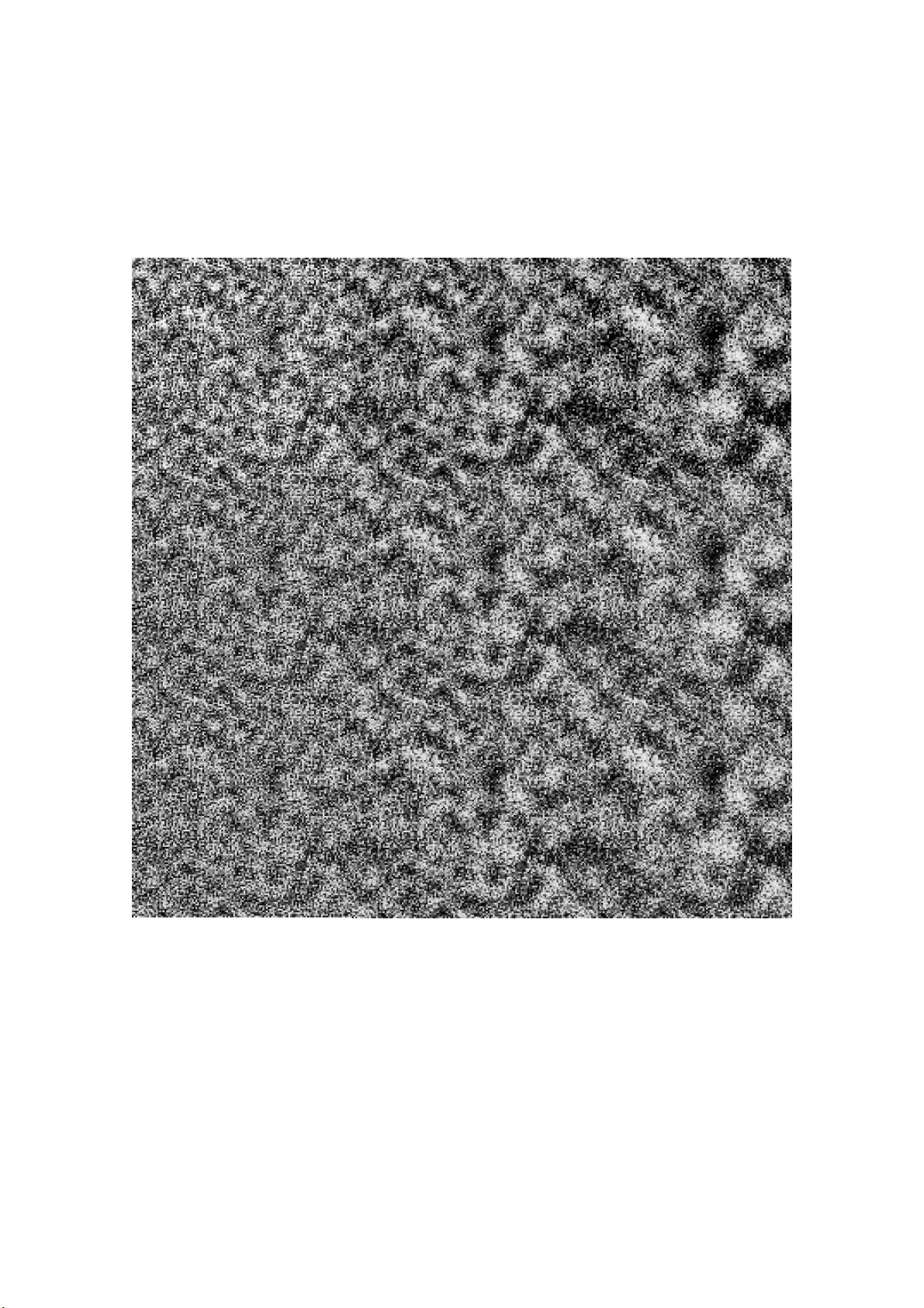
Sampling Spatially Correlated Clutter Oscar H. Bustos 1 Ana Georgina Flesia 1 Alejandro C. F rery 2 Mar ´ ıa Magdalena Lucini 3 Octob er 25, 2018 1 F acultad de Matem´ atica Astronom ´ ıa y F ´ ısica, Un iv ersidad Nacional de C´ ordoba, Ing. Medina A llend e esq. H a y a de la T orre, 5000 C´ ordoba, Argentina, F ax: 54-351-4334 054, { bustos,flesi a } @mate.un cor.edu 2 Universidade F ederal de Alagoas, Instituto de Computa¸ c˜ ao, Campus A. C. Simes, BR 104 - N orte, K m 97, T abu leiro dos Martins - Macei´ o - A L , CEP 57072-970. acfr ery@pesquis ador.cnpq.b r 3 Universidad Nacional de Nordeste, F acultad de Ciencias Exactas, Naturales y Agrimensura, Av. Lib ertad 5450 - Campus ”Deo doro Ro ca”, (3400) Corrientes, T el: +54 (3783) 473931/473 932 lucini@exa .unne.edu.a r Abstract Correla ted G distributions can be used to describ e the clutter seen in images obtained with coher en t illumination, as is the case of B -scan ultrasound, laser, sonar and synthetic ape r ture radar (SAR) ima gery . These distributions are derived using the square ro ot of the genera lized in verse Gauss ia n distribution for the amplitude backscatter within the m ultiplicativ e mo del. A t w o-para meters particular case of the a mplitude G distribution, called G 0 A , constitutes a modeling improvemen t with r e s pect to the widespr ead K A distribution when fitting ur ban, forested and defor ested ar eas in remote s ensing data. This ar ticle deals with the mo deling and the simulation of co rrelated G 0 A -distributed ra ndom fields. It is accomplished by means of the In v erse T r ansform metho d, applied to Ga ussian random fields with spatial cor relation. The main feature o f this a pproach is its genera lit y , since it allows the intro duction of negative c o rrelation v alues in the r esulting pro cess, necessa r y for the prop er explanation of the shadowing effect in many SAR ima g es. Keyw ords: imag e mo deling, simulation, spatia l cor relation, sp eckle. 1 In tro duction The demand fo r exha ustiv e a nd controlled clutter measur emen ts in all scenarios would b e alleviated if plausible data could b e obtained b y c omputer simulation. Clutter simulation is an impo rtan t element in the developmen t of ta rget detection algor ithms for radar , sona r, ultraso und and laser imaging systems. Using simulated data, the accuracy o f clutter mo dels may be assessed a nd the p erformance of tar get detection algorithms ma y b e quantified with controlled clutter backgrounds. This article is c o ncerned with the simulation of random clutter having appro priate b oth first and s econd o r der statistical pr oper ties . The use of correla tion in clutter mo dels is significant and relev an t since the co r relation effects within the clutter often dominate system per formance. Mo dels merely based on sing le-point statistics could, therefore, pro duce misleading res ults, and several co mmonly used for ms for clutter statistics fall into this categor y . The statistical pro perties of heter ogeneous clutter returned by Syn thetic Ape r ture Radar (SAR) senso rs hav e b een largely inv estigated in the literatur e. A theoretical model widely adopted for these images a ssumes that the v alue in every pixel is the observ ation of an uncorrelated sto c hastic pro cess Z A , characterized by single- po in t (firs t order) sta tis tics . A gener a l agreement has been reached that amplitude fields are well explained by the K A distribution. Such distribution arises when coher en t ra diation is scattered by a surface having Gamma-distributed cr oss-section fluctuations. Though agr icultural fields a nd wo odla nd are very well fitted by this dis tribution, it is also known that it fails giving a ccurate statistical descr iption of ex tr emely heterogeneous data, such a s ur ban ar eas and fore st gr owing o n undulated r elief. As discussed in [1, 2], ano ther distribution, the G A law, c a n b e used to descr ibe those extremely heterog eneous regions, with the adv antage that it has the K A distribution as a particula r ca se. This distribution arises in all coherent imaging applications as a r esult of the action o f multiplicativ e speckle no ise on an underlying square ro ot of a generalized inv erse Gaussia n distr ibution. The main dr a wback of this general mo del is that it requir es an extra para meter, b esides its theor etical co mplexit y . Nevertheless, it can b e seen in [3, 4, 5] that a sp ecial ca se of the G A distribution, namely the G 0 A law, which has a s many par ameters as the K A distribution, is able to mo del with a ccuracy every type of clutter. As a conseq ue nce , effo r ts have bee n directed toward the simulation of G 0 A textures, but no exa ct metho d for generating patterns with arbitrary spa tia l auto corr elation functions has been envisaged so far, in spite of it being more tracta ble than the K A distribution. As previously stated, spatial co r relation is ne e ded in order to increas e the a dequacy of the mo del to rea l situations. This pap er ta c kles the pr oblem o f sim ulating corr elated G 0 A fields. 2 Correlated G 0 A clutter The main prop erties a nd definitions o f the G 0 A clutter are prese nted in this section, starting with the first or der prop erties of the distributio n and concluding with the definition o f a G 0 A sto c hastic pro cess tha t will des cribe Z A fields. 2.1 Marginal prop erties The G 0 A ( α, γ , n ) distribution is c haracter ized by the following probability density function: f Z A ( z , ( α, γ , n )) = 2 n n Γ( n − α ) √ γ Γ( − α )Γ( n ) ·  z √ γ  2 n − 1  1 + z 2 γ n  n − α · I (0 , + ∞ ) ( z ) , α < 0 , γ > 0 , (1) being n ≥ 1 the num ber of lo oks of the image, whic h is controlled at the imag e g eneration pro cess, and I T ( · ) the indicator function of the set T . The pa rameter α descr ibes the r oughness, being small v alues (say α ≤ − 15 ) usually ass ocia ted to ho mogeneous targets, lik e pasture, v alues rang ing in the ( − 1 5 , − 5] interv al usually o bserved 1 in heteroge neous clutter, like forests, and big v alues ( − 5 < α < 0 for insta nce ) commonly seen when extremely heterogeneo us area s are imaged. The para meter γ is related to the scale, in the sense that if Z is G 0 A ( α, 1 , n ) distributed then Z A = √ γ Z obeys a G 0 A ( α, γ , n ) law. A SAR image o ver a suburban area of M¨ unch en, Germany , is shown in Fig ur e 1. It w as obtained with E-SAR, an exp erimental po la rimetric airb orne sensor op e rated by the German Aer ospace Agency (Deutsc hes Zentrum f ¨ ur Luft- und Raumfahrt – DLR e. V.) The da ta here shown were generated in single look fo rmat, and e x hibit the thre e discussed t ype s of r oughness: homo geneous (the dark areas to the middle of the imag e), heterogeneo us (the clear ar ea to the left) a nd extremely heteroge neo us (the clear area to the right). Figure 1: E-SAR image showing three types of texture. 2 The r -th moment s of the G 0 A ( α, γ , n ) distribution are E ( Z r A ) =  γ n  r 2 Γ( − α − r 2 )Γ( n + r 2 ) Γ( − α )Γ( n ) , α < − r / 2 , n ≥ 1 , (2) when − r/ 2 ≤ α < 0 the r -th order moment is infinite. Using eq uation (2) the mean a nd v ariance of a G 0 A ( α, γ , n ) distributed rando m v ariable can be computed: µ Z A = r γ n Γ( n + 1 2 )Γ( − α − 1 2 ) Γ( n )Γ( − α ) , σ 2 Z A = γ  n Γ 2 ( n )( − α − 1)Γ 2 ( − α − 1 ) − Γ 2 ( n + 1 2 )Γ 2 ( − α − 1 2 )  n Γ 2 ( n )Γ 2 ( − α ) . Figure 2 shows thr e e densities of the G 0 A ( α, γ , n ) distr ibution for the single lo ok ( n = 1) case. These densities are normaliz e d so that the expe cted v alue is 1 for every v alue of the roughness parameter. This is obta ined using equation (2) for setting the sca le para meter γ = γ α,n = n (Γ( − a )Γ( n ) / (Γ( − a − 1 / 2 )Γ( n + 1 / 2))) 2 . These densi- ties illustrate the three t ypical situations describ ed ab ov e: ho mogeneous areas ( α = − 1 5 , dashes), heterog eneous clutter ( α = − 5, dots) and an extremely heterogeneo us target ( α = − 1 . 5, solid line). Figure 2: Densities of the G 0 A ( α, γ α, 3 , 3) distribution. F ollowing Barndor ff-Nielsen and Blæsild [6], it is interesting to s ee these densities as lo g proba bilit y functions, particularly b ecause the G 0 A is closely related to the c la ss of Hyp erb olic distributions [7]. Fig ure 3 shows the 3 densities of the G 0 A ( − 3 , 1 , 1 ) and N (3 π / 16 , 1 / 2 − 9 π 2 / 256) distributions in semilogarithmic scale, along with their mean v a lue µ = 3 π / 16 . The parameters were chosen so that these distributions ha v e equal mean and v ar iance. The different deca ys of their tails is ev iden t: the for mer behaves logarithmically , while the latter decays quadratically . This behavior ensur es the ability of the G 0 A distribution to mo del data with ex tr eme v ar iabilit y . Figure 3 : Densities of the G 0 A and Gaussian distributions with same mean v alues µ = 3 π / 16 in se milogarithmic scale. Besides being essential for the simulation technique here prop osed, cumulativ e distribution functions are needed for carrying out g oo dness of fit tests and for the prop osal o f es timators based on o rder statistics. It can b e seen in [3, 8, 9] that the cum ulative distribution function of a G 0 A ( α, γ , n ) dis tr ibuted rando m v ariable is given, for every z > 0, by G ( z , ( α, γ , n )) = Υ 2 n, − 2 α ( − αz 2 /γ ), where Υ s,t is the cumulativ e distribution function of a Snedecor’s F s,t distributed random v ariable with s a nd t degrees of freedom. Both Υ · , · and Υ − 1 · , · are r eadily av ailable in most platforms for c omputational statistics. The single lo ok case is of particular interest since it descr ibes the noisiest imag es and it exhibits nice analytical prop erties. The distribution is characterized b y the density f ( z ; α, γ , 1) = − 2 α γ α z ( γ + z 2 ) α − 1 I (0 , ∞ ) ( z ), whith − α, γ > 0. Its cumulativ e distribution function is giv en b y F ( t ) = 1 −  1 + t 2 /γ  α I (0 , ∞ ) ( t ), and its inv erse, useful for the gener ation of r andom deviates and the computation of quantiles, is given by F − 1 ( t ) =  γ  (1 − t ) 1 /α − 1  1 / 2 I (0 , 1) ( t ). 4 2.2 Correlated clutter Instead of defining the mo del ov er Z 2 , in this section a rea listic description of finite-sized fields is made. Let Z A = ( Z A ( k , ℓ )) 0 ≤ k ≤ N − 1 , 0 ≤ ℓ ≤ N − 1 be the sto c hastic mo del that descr ib es the retur n amplitude imag e. Definition 1 We say that Z A is a G 0 A ( α, γ , n ) sto cha stic pr o c ess with c orr elation funct ion ρ Z A (in symb ols Z A ∼ ( G 0 A ( α, γ , n ) , ρ Z A ) ) if for al l 0 ≤ i, j, k , ℓ ≤ N − 1 holds that 1. Z A ( k , ℓ ) ob eys a G 0 A ( α, γ , n ) law; 2. the me an field is µ Z A = E ( Z A ( k , ℓ )) ; 3. the varianc e field is σ 2 Z A = V ar ( Z A ( k , ℓ )) ; 4. the c orr elation function is ρ Z A (( i, j ) , ( k , ℓ )) =  E ( Z A ( i, j ) Z A ( k , ℓ )) − µ 2 Z A  /σ 2 Z A . The sc a le prop erty of the para meter γ implies that cor relation function ρ Z A and γ are unrela ted a nd, therefore, it is enough to g enerate a Z 1 A ∼ ( G 0 A ( α, 1 , n ) , ρ Z A ) field and then simply mult iply every outco me by γ 1 / 2 to get the desir ed field. This pap er presents a v ariation of a metho d used for simulation of cor related Gamma v ariables, called T ra nsformation Me tho d, that can b e found in [10]. This metho d can b e summarized in the following three steps: 1. Generate indep endent outcomes fro m a conv enien t distribution. 2. Introduce cor relation in these da ta . 3. T ransform the corr elated obser v ations in to data with the desired marginal prop erties [11]. The trans formation that guarantees the v alidit y of this pr o cedure is obtained fro m the cum ulative distribu- tion functions o f the data obtained in step 2, a nd from the des ired set of distributions. Recall that if U is a contin uous random v ar iable with cum ulative dis tribution function F U then F U ( U ) ob eys a uniform U (0 , 1) law and, recipro cally , if V obeys a U (0 , 1) distribution then F − 1 U ( V ) is F U distributed. In order to use this metho d it is necessary to know the cor relation that the r andom v ariables will hav e after the transformatio n, be sides the function F − 1 U . The metho d here studied cons is ts of the following steps: 1. prop ose a cor relation structure for the G 0 A field, say , the function ρ Z A ; 2. genera te a field of indep endent identically distributed sta nda rd Gaussian o bs erv ations; 3. compute τ , the cor relation structure to b e imp osed to the Gaussian field from ρ Z A , and impa ir it using the F o urier transform without altering the marginal prop erties; 4. transfor m the correla ted Gaussian field into a field o f obser v ations of iden tically distributed U (0 , 1) r andom v ar iables, using the cum ulative distribution function o f the Gaussian distribution (Φ); 5. transfor m the uniform observ atio ns in to G 0 A outcomes, using the inv erse of the cumu lative distribution function of the G 0 A distribution ( G − 1 ). The function that relates ρ Z A and τ is computed using n umerical to ols. In principle, there are no r e strictions on the p ossible ro ughness parameter s v alues that can b e o bta ined by this metho d, but issues rela ted to machine precision must be tak en into account. Another imp ortant issue is that not every desired final correla tion structure ρ Z A is mapp ed onto a feasible in termediate correla tion structur e τ . The pro cedure is pres en ted in detail in the nex t s ection. 5 3 T ransformation M etho d Let G ( · , ( α, γ , n )) b e the cumulativ e distribution function of a G 0 A ( α, γ , n ) distributed r andom v a riable. As previously stated, G ( x, ( α, γ , n )) = Υ 2 n, − 2 α  − αx 2 γ  , where Υ ν 1 ,ν 2 is the cumulativ e distribution function of a Snedecor F ν 1 ,ν 2 distribution, i.e., Υ ν 1 ,ν 2 ( x ) = Γ  ν 1 + ν 2 2  Γ  ν 1 2  Γ  ν 2 2   ν 1 ν 2  ν 1 2 Z x 0 t ν 1 − 2 2  1 + ν 1 ν 2 t  − ν 1 + ν 2 2 dt. The inv erse of G ( · , ( α, γ , n )) is, therefore, G − 1 ( t, ( α, γ , n )) = r − γ α Υ − 1 2 n, − 2 α ( t ) . T o generate Z 1 A = ( Z 1 A ( k , ℓ )) 0 ≤ k ≤ N − 1 , 0 ≤ ℓ ≤ N − 1 ∼ ( G 0 A ( α, 1 , n ) , ρ Z A ) using the inv ersion metho d w e define ev- ery co ordina te of the pro cess Z A as a trans formation of a Gauss ian pro cess ζ as Z 1 A ( i, j ) = G − 1 (Φ( ζ ( i, j )) , ( α, 1 , n )), where ζ = ( ζ ( i, j )) 0 ≤ i ≤ N − 1 , 0 ≤ j ≤ N − 1 is a sto chastic pro cess such that ζ ( i, j ) is a sta ndard Gauss ian rando m v a ri- able and with co r relation function τ ζ (i.e. where τ ζ (( i, j ) , ( k , ℓ )) = E ( ζ ( i, j ) ζ ( k, ℓ ))) satisfying ρ Z A (( i, j ) , ( k , ℓ )) =  ( α,n ) ( τ ζ (( i, j ) , ( k , ℓ ))) (3) for all 0 ≤ i, j, k , ℓ ≤ N − 1 and ( i, j ) 6 = ( k , ℓ ) and where Φ denotes the cumulativ e distribution function o f a standard Gaussia n ra ndom v ar iable. Posed a s a diagr am, the metho d co nsists of the following transformatio ns among Gaussian ( N ), Uniform ( U ) and G 0 A -distributed ra ndom v ar iables: N U G 0 A ✲ Φ ❄ G − 1 A central issue of the metho d is finding the corr elation s tructure that the Gaussia n field has to obey , in order to hav e the desired G 0 A field a fter the transfor mation. The function  ( α,n ) is defined on ( − 1 , 1) by  ( α,n ) ( τ ) = R ( α,n ) ( τ ) −  1 n   Γ( n + 1 2 )Γ( − α − 1 2 ) Γ( n )Γ( − α )  2 − 1 1+ α −  1 n   Γ( n + 1 2 )Γ( − α − 1 2 ) Γ( n )Γ( − α )  2 , with R ( α,n ) ( τ ) = Z Z R 2 G − 1 (Φ( u ) , ( α, 1 , n )) G − 1 (Φ( v ) , ( α, 1 , n )) φ 2 ( u, v , τ ))) dudv = 1 | α | 2 π √ 1 − τ 2 Z Z R 2 q Υ − 1 2 n, − 2 α (Φ( u )) . Υ − 1 2 n, − 2 α (Φ( v )) exp  − u 2 − 2 τ .u.v + v 2 2(1 − τ 2 )  dudv , where φ 2 ( u, v , τ ) = 1 2 π p (1 − τ 2 ) exp  − u 2 − 2 τ .u.v + v 2 2(1 − τ 2 )  . Note that R ( α,n ) ( τ ζ (( i, j ) , ( k , ℓ ))) = E ( Z 1 A ( i, j ) Z 1 A ( k , ℓ )) for all 0 ≤ i , j, k , ℓ ≤ N − 1 and ( i, j ) 6 = ( k , ℓ ). The a nsw er to the question of finding τ ζ given ρ Z A is equiv alent to the problem of inverting the function  ( α,n ) . This function is only av ailable using numerical metho ds, an approximation that may impo se restrictions on the use of this simulation metho d. 6 3.1 In v ersion of  ( α,n ) The function  ( α,n ) has the following prop erties: 1. The set {  ( α,n ) ( τ ) : τ ∈ ( − 1 , 1 ) } is s trictly included in ( − 1 , 1), and dep ends on the v alues of α . 2. The function  ( α,n ) is strictly increa sing in ( − 1 , 1). 3. The v alues  ( α,n ) ( τ ) are strictly neg ativ e for a ll τ < 0 . Let ð ( α,n ) be the in verse function of  ( α,n ) . Then, in order to calculate its v alue for a fixed ρ ∈ ( − 1 , 1), we hav e to solve the following equation in τ : R ( α,n ) ( τ ) + ρ 1 + α + ( ρ − 1)  1 n   Γ( n + 1 2 )Γ( − α − 1 2 ) Γ( n )Γ( − α )  2 = 0 Then, it follows from the prop erties of  ( α,n ) , that for cer ta in v alues of α the set of τ such that this equation is solv a ble is a s tr ict subset of ( − 1 , 1). T able 1 shows s ome v a lues of the function ð ( α,n ) for sp ecific v a lues o f ρ , n and α . Figure 4 s hows τ a s a function of ρ for the n = 1 case and v arying v alues of α , a nd it can b e s een that the smaller α the clo ser this function is to the identit y . This is s ensible, since the G 0 A distribution beco mes more and mo re symmetric as α → −∞ and, therefore, simulating outcomes from this distribution b ecomes clo ser and closer to the pro blem of obtaining Gaussian deviates. Figure 5 presents the same function for α = − 1 . 5 and v arying num ber of lo oks. It is noticea ble that τ is far less sensitive to n than to α , a feature that sug gests a shortcut for computing the v alues of T able 1: disr egarding the dep endence on n , i.e., co nsidering τ ( ρ, α, n ) ≃ τ ( ρ, α, n 0 ) for a fixed conv enient n 0 . The so urce FOR TRAN file with r outines for computing the functions  ( α,n ) and ð ( α,n ) can be obtained from the first a utho r of this pa per. 3.2 Generation of the pro cess ζ The pr o cess ζ , that consists of spatially correla ted standa rd Gaussian r andom v a riables, will b e g enerated using a sp ectral technique that employs the F ourier transform. This metho d has computational adv an tages with resp ect to the direct application o f a conv olution filter . Again, the co ncern here is to define a finite proce s s instead of working o n Z 2 for the sake of simplicity . Consider the following sets : R 1 = { ( k , ℓ ) : 0 ≤ k , ℓ ≤ N / 2 } , R 2 = { ( k , ℓ ) : N / 2 + 1 ≤ k ≤ N − 1 , 0 ≤ ℓ ≤ N / 2 } , R 3 = { ( k , ℓ ) : 0 ≤ k ≤ N / 2 , N / 2 + 1 ≤ ℓ ≤ N − 1 } , R 4 = { ( k , ℓ ) : N / 2 + 1 ≤ k ≤ N − 1 , N/ 2 + 1 ≤ ℓ ≤ N − 1 } , R N = R 1 ∪ R 2 ∪ R 3 ∪ R 4 = { ( k , ℓ ) : 0 ≤ k , ℓ ≤ N − 1 } , R N = { ( k , ℓ ) : − ( N − 1) ≤ k , ℓ ≤ N − 1 } . Let ρ : R 1 − → ( − 1 , 1) b e a function, extended ont o R N by: ρ ( k , ℓ ) =                ρ ( N − k , ℓ ) if ( k , ℓ ) ∈ R 2 , ρ ( k , N − ℓ ) if ( k , ℓ ) ∈ R 3 , ρ ( N − k , N − ℓ ) if ( k , ℓ ) ∈ R 4 , ρ ( N + k , ℓ ) if − ( N − 1) ≤ k < 0 ≤ ℓ ≤ N − 1 , ρ ( k , N + ℓ ) if − ( N − 1) ≤ ℓ < 0 ≤ k ≤ N − 1 , ρ ( N + k , N + ℓ ) if − ( N − 1) ≤ k , ℓ < 0 . 7 h ρ α = − 1 . 5 α = − 3 . 0 α = − 9 . 0 n = 1 n = 3 n = 6 n = 1 0 n = 1 n = 3 n = 6 n = 10 n = 1 n = 3 n = 6 n = 10 − . 9 − . 953 − . 954 − . 958 − . 8 − . 877 − . 845 − . 845 − . 848 − . 7 − . 886 − . 881 − . 901 − . 915 − . 763 − . 737 − . 737 − . 740 − . 6 − . 747 − . 745 − . 761 − . 772 − . 650 − . 630 − . 630 − . 632 − . 5 − . 613 − . 612 − . 624 − . 632 − . 539 − . 523 − . 523 − . 525 − . 4 − . 844 − . 903 − .9 48 − . 9 72 − . 483 − . 4 83 − . 492 − . 498 − . 4 2 9 − . 417 − . 417 − . 419 − . 3 − . 591 − . 630 − .6 5 6 − . 67 0 − . 357 − . 35 7 − . 363 − . 367 − . 32 0 − . 312 − . 312 − . 31 3 − . 2 − . 370 − . 392 − .4 05 − . 4 12 − . 234 − . 2 35 − . 239 − . 241 − . 2 1 2 − . 207 − . 207 − . 208 − . 1 − . 174 − . 183 − .1 88 − . 1 90 − . 116 − . 1 16 − . 117 − . 119 − . 1 0 5 − . 103 − . 103 − . 104 0 . 0 . 0 .0 . 0 . 0 . 0 . 0 . 0 . 0 . 0 . 0 . 0 . 1 . 155 . 161 .164 . 165 . 11 2 . 113 . 11 4 . 115 . 1 04 . 103 . 1 03 . 10 3 . 2 . 294 . 303 .307 . 3 09 . 222 . 223 . 22 5 . 226 . 2 08 . 205 . 2 05 . 20 5 . 3 . 418 . 428 .433 . 4 35 . 328 . 329 . 33 2 . 334 . 3 10 . 306 . 3 06 . 30 7 . 4 . 529 . 539 .544 . 5 46 . 432 . 433 . 43 6 . 438 . 4 11 . 407 . 4 07 . 40 8 . 5 . 629 . 638 .642 . 6 44 . 533 . 534 . 53 7 . 539 . 5 12 . 507 . 5 08 . 50 8 . 6 . 719 . 727 .730 . 7 31 . 631 . 633 . 63 5 . 637 . 6 11 . 607 . 6 07 . 60 8 . 7 . 800 . 806 .808 . 8 09 . 727 . 728 . 73 1 . 732 . 7 10 . 706 . 7 06 . 70 7 . 8 . 873 . 877 .879 . 8 80 . 820 . 821 . 82 3 . 824 . 8 07 . 805 . 8 05 . 80 5 . 9 . 940 . 942 .942 . 9 43 . 911 . 912 . 91 3 . 913 . 9 04 . 903 . 9 03 . 90 3 T able 1: V alues o f function ð ( α,n ) . 8 Let Z A = ( Z A ( k , ℓ )) 0 ≤ k ≤ N − 1 , 0 ≤ l ≤ N − 1 be a G 0 A ( α, γ , n ) sto chastic pro cess with corr e lation function ρ Z A defined by ρ Z A (( k 1 , ℓ 1 ) , ( k 2 , ℓ 2 )) = ρ ( k 2 − k 1 , ℓ 2 − ℓ 1 ) . Assume that τ ( k , ℓ ) = ð ( α,n ) ( ρ ( k , ℓ )) is defined for a ll ( k , ℓ ) in R N . Let F ( τ ) : R N − → C b e the nor ma lized F o urier T ra nsform of τ , that is, F ( τ )( k , ℓ ) = 1 N 2 N − 1 X k 1 =0 N − 1 X ℓ 1 =0 τ ( k 1 , ℓ 1 ) exp( − 2 π i ( k · k 1 + ℓ · ℓ 1 ) / N 2 ) . Let ψ : R N − → C b e de fined by ψ ( k , ℓ ) = p F ( τ )( k , ℓ ) a nd let the function θ : R N = { ( k , ℓ ) : − ( N − 1) ≤ k , ℓ ≤ N − 1 } − → R be defined by θ ( k , ℓ ) = F − 1 ( ψ )( k, ℓ ) / N = 1 N N − 1 X k 1 =0 N − 1 X ℓ 1 =0 ψ ( k 1 , ℓ 1 ) exp(2 π i ( k · k 1 + ℓ · ℓ 1 ) / N 2 ) , (the nor malized inv erse F ourier T ransfo r m of ψ ) for all ( k , ℓ ) ∈ R N ; a nd θ ( k , ℓ ) =    θ ( N + k , ℓ ) if − ( N − 1) ≤ k < 0 ≤ ℓ ≤ N − 1 , θ ( k , N + ℓ ) if − ( N − 1) ≤ ℓ < 0 ≤ k ≤ N − 1 , θ ( N + k , N + ℓ ) if − ( N − 1) ≤ k , ℓ < 0 . A straightforward ca lculation shows that ( θ ∗ θ )( k , ℓ ) = N − 1 X k 1 =0 N − 1 X ℓ 1 =0 θ ( k 1 , ℓ 1 ) θ ( k − k 1 , ℓ − ℓ 1 ) = τ ( k , ℓ ) , for all ( k , ℓ ) ∈ R N . Remark 1 We c an se e that F ( τ )( k , ℓ ) ≥ 0 and the last e quality for al l ( k , ℓ ) ∈ R N is e asily de duc e d fr om the r esults in Se ction 5.5 of [12]; mor e details c an b e se en in [13]. Finally we define ζ = ( ζ ( i, j )) 0 ≤ i ≤ N − 1 , 0 ≤ j ≤ N − 1 by ζ ( k, ℓ ) = ( θ ∗ ξ )( k , ℓ ) = N F − 1 (( ψ F ( ξ )))( k , ℓ ) , where ξ = ( ξ ( k , ℓ )) ( k,ℓ ) . ∈ R N is a Gaussian white nois e with sta nda rd devia tion 1. Then it is easy to prov e that ζ = ( ζ ( i, j )) 0 ≤ i ≤ N − 1 , 0 ≤ j ≤ N − 1 is a sto c hastic pro cess suc h that ζ ( i, j ) is a standard Gaussia n ra ndom v ar iable with correlatio n function τ ζ satisfying (3). 3.3 Implemen t ation The results prese n ted in previous sections were implemen ted using the IDL V ersio n 5.3 Win 3 2 [14] developmen t platform, with the following algorithm: Algorithm 1 Input: α < − 1 , γ > 0 , n ≥ 1 inte ger, ρ and τ funct ions as ab ove, then: 1. Compute the fr e quency domain m ask ψ ( k , ℓ ) = p F ( τ )( k , ℓ ) . 2. Gener ate ξ = ( ξ ( k , ℓ )) ( k,ℓ ) ∈ R N , the Gaussian white noise with zer o me an and varianc e 1 . 3. Calculate ζ ( k , ℓ ) = N F − 1 (( ψ · F ( ξ )))( k , ℓ ) , for every ( k , ℓ ) . 4. Obtain Z 1 A ( k , ℓ ) = G − 1 (Φ( ζ ( k, ℓ )) , ( α, 1 , n )) , for every ( k , ℓ ) . 5. R eturn Z A ( k , ℓ ) = √ γ Z 1 A ( k , ℓ ) for every ( k , ℓ ) . 9 4 Sim u latio n results In practice b oth para metric and non-par ametric cor relation structures ar e of interest. The former rely on ana- lytic forms fo r ρ , while the latter merely sp ecify v alues for the correla tion. Parametric for ms for the corr elation structure are simpler to spe cify , and its inference amounts to estimating a few numerical v a lues; non-pa rametric forms do not suffer fr om lack of adequac y , but demand the sp ecification (and p ossibly the estima tio n) of po - ten tially lar ge sets of pa rameters. In the following examples the technique presented ab ov e will b e used to ge ne r ate samples from both par a- metric and non-pa r ametric cor relation str uctures. Example 1 (P arametric situation) Thi s c orr elation mo del is very p opular in applic ations. Consider L ≥ 2 an even inte ger, 0 < a < 1 , 0 < ε (for example ε = 0 . 001 ), α < − 1 and n ≥ 1 . L et h : R − → R b e define d by h ( x ) =  x if | x | ≥ ε , 0 if | x | < ε. L et ρ : R 1 − → ( − 1 , 1) b e define d by ρ (0 , 0 ) = 1 if ( k , ℓ ) 6 = (0 , 0 ) in R 1 by: ρ ( k , ℓ ) =  h ( a exp( − k 2 /L 2 )) if k ≥ ℓ, − h ( a exp( − ℓ 2 /L 2 )) if k < ℓ. The image shown in Figur e 6, of size 128 × 1 28 , was obtaine d assuming a = 0 . 4 , L = 2 , α = − 1 . 5 , γ = 1 . 0 and n = 1 . Example 2 (Mos ai c) A m osaic of nine simulate d fields is shown in Figur e 7. Each field is of size 1 28 × 12 8 and ob eys the m o del pr esente d in Example 1 with a = 0 . 4 , γ = 1 . 0 , n = 1 , r oughness α varying in the r ows ( − 1 . 5 , − 3 . 0 and − 9 . 0 fr om t op to b ottom) and c orr elation length L varying along the c olumns ( 2 , 4 and 8 fr om left to right). Example 3 (Non-parametric situation) The starting p oint is the urb an ar e a se en in Figur e 8. This 1 2 8 × 128 pixels image is a smal l sample of data obtai ne d by the E-SAR system over an u rb an ar e a. The c omplete dataset was use d as input for estimating the c orr elation stru ct ur e define d by an 16 × 16 c orr elation m atrix using Pe arson ’s pr o c e dur e ( ˆ ρ b elow, wher e only values bigger than 10 − 3 ar e shown; se e app endix A). The c orr elation structur e for the Gaussian pr o c ess is τ b elow, wher e only values bigger than 10 − 3 ar e shown. The r oughness and sc ale p ar ameters wer e estimate d using the moments te chnique. The simulate d G 0 A field is shown in Figur e 9 . ˆ ρ =                         1 . 00 0 . 65 0 . 22 0 . 97 0 . 63 0 . 22 0 . 88 0 . 58 0 . 21 0 . 76 0 . 50 0 . 19 0 . 64 0 . 43 0 . 16 0 . 53 0 . 36 0 . 14 0 . 43 0 . 30 0 . 12 0 . 36 0 . 25 0 . 10 0 . 29 0 . 20 0 . 00 0 . 24 0 . 17 0 . 00 0 . 20 0 . 13 0 . 00 0 . 16 0 . 11 0 . 00 0 . 13 0 . 00 0 . 00 0 . 11 0 . 00 0 . 00                         , τ =                         1 . 00 0 . 76 0 . 32 0 . 98 0 . 74 0 . 32 0 . 93 0 . 70 0 . 31 0 . 85 0 . 63 0 . 28 0 . 75 0 . 56 0 . 24 0 . 68 0 . 49 0 . 21 0 . 56 0 . 42 0 . 18 0 . 49 0 . 36 0 . 16 0 . 41 0 . 294 0 . 00 0 . 35 0 . 25 0 . 00 0 . 29 0 . 20 0 . 00 0 . 24 0 . 17 0 . 00 0 . 20 0 . 00 0 . 00 0 . 17 0 . 00 0 . 00                         10 5 Conclusions and future w ork A metho d for the simulation of cor related clutter with desirable marginal law and correlation structure w as presented. This metho d a llo ws the obtainment o f pr e c ise a nd controlled first and second order statistics, and can b e easily implemented using standard nu merical to ols. The adequacy of the metho d for the simulation of several scenar ios will b e as sessed using real data, following the pro cedure presen ted in E xample 3: estimating the under lying correlation structur e and then simulating fields with it. A mosaic of tr ue and synthetic textures will b e comp osed and made av aila ble for use in a lgorithm assessment. Ac kno wledgemen ts This work was partially suppo rted by Conicor and SeCyT (Arg en tina) and CNPq (Brazil). References [1] A. C. F rer y , H.-J. M ¨ uller, C. C . F. Y ana sse, and S. J . S. Sant’Anna. A mo del for e x tremely heterog eneous clutter. IEEE T r ansactions on Ge oscienc e and R emote Sensing , 3 5(3):648–6 5 9, May 199 7. [2] A. C. F rery , A. H. Cor r eia, C. D. Renn´ o, C. C. F reitas, J. Jaco bo-Be rlles, M. E. Me ja il, a nd K. L. P . V asc o ncellos. Mo dels for synthetic ap erture radar image analy sis. R esenhas (IME-US P) , 4(1 ):45–77, 1 999. [3] M. E . Mejail, A. C. F rery , J. Ja cobo -Berlles, and O. H. Bus tos. Approximation of dis tributions for SAR images: prop osal, ev alua tion a nd pra ctical consequences. L atin Americ an Applie d Re se ar ch , 31:83–9 2, 200 1. [4] O. H. Bustos, M. M. Lucini, and A. C. F rery . M-estimators of roughness and scale for GA0 - modelled SAR imagery . EURASIP Journal on A ppli e d Signal Pr o c essing , 2002(1):10 5–114, Jan. 2002 . [5] F. Cr ibari-Neto, A. C. F rery , a nd M. F. Silv a. Impr o ved estimation of clutter prop erties in sp eckled imagery . Computational Statistics and Data Analysis , 40(4):80 1 –824, 2002 . [6] O. E. Ba rndorff-Nielsen and P . Blæsild. Hyperb olic distributions and ra mifications: Contributions to theory and applications. In C. T a illie and B. A. Baldessar i, editors , Statistic al distributions in scientific work , pages 19– 44. Reidel, Dordre c h t, 1 981. [7] A. C. F rer y , C. C. F. Y a nasse, a nd S. J. S. San t’Anna. Alternative distributions for the mult iplicative mo del in SAR images . In International Ge osci enc e and Remote Sensing Symp osium: Qu antitative R emote R ensing for Scienc e and Applic ations , pages 1 69–171, Florence, Jul. 1995. IEEE Computer So ciety . IGARSS’95 Pro c. [8] M. E . Mejail, J. C. J acobo -Berlles, A. C. F rery , a nd O. H. B ustos. Cla ssification of SAR ima g es using a general and tra c table mult iplicative mo del. International Journal of R emote Sensing . In pre ss. [9] M. E. Mejail, J. Jacob o-Berlle s , A. C. F rery , a nd O. H. Bustos. Parametric r oughness estimation in amplitude SAR images under the m ultiplicative mo del. R evista de T ele dete c ci´ o n , 13:37–4 9, 20 0 0. [10] O. H. Bustos, A. G. Flesia, and A. C. F rer y . Generalized metho d for sampling spatia lly corr e lated heter o- geneous sp eckled imager y . EURASIP Journal on Applie d Signal Pr o c essing , 2001 (2):89–99, June 200 1. [11] C. O liv er a nd S. Queg an. Understanding S ynthetic Ap ertur e R adar Images . Artech House, Boston, 19 98. 11 [12] A. K. Jain. F u ndamentals of Digital Image Pr o c essing . Pr e ntice-Hall International E ditions, Englewoo d Cliffs, NJ, 19 89. [13] S. M. Kay . Mo dern Sp e ct ra l Est imation: The ory & A pplic ation . Prentice Hall, Englewo od Cliffs, NJ, USA, 1988. [14] Resea rc h Systems. Using IDL . htt p://www.rs inc.com, 1999 . A Estimating correlation structure with Pe arson’s metho d Consider the imag e z with M r o ws a nd N c o lumns z =    z (0 , 0 ) · · · z ( N − 1 , 0) . . . . . . . . . z (0 , M − 1 ) · · · z ( N − 1 , M − 1)    and n v a po s itiv e integer sma lle r than min( M , N ). Define n c = [ N / (2 n v )] and n f = [ M / (2 n v )], where [ x ] = max { k ∈ N : k ≤ x } for e v ery real num ber x . F or each i = 0 , . . . , n c − 1 and ea c h j = 0 , . . . , n f − 1 define c ( i, j ) the submatrix of z of size 2 n v × 2 n v given b y c ( i, j ) =    z (2 n v i, 2 n v j ) · · · z (2 n v i + 2 n v − 1 , 2 n v j ) . . . . . . . . . z (2 n v i, 2 n v j + 2 n v − 1) · · · z (2 n v i + 2 n v − 1 , 2 n v j + 2 n v − 1)    , and let z v ( i, j ) b e the submatrix of c ( i, j ) o f siz e n v × n v given b y z v ( i, j ) =    z (2 n v i, 2 n v j ) · · · z (2 n v i + n v − 1 , 2 n v j ) . . . . . . . . . z (2 n v i, 2 n v j + n v − 1) · · · z (2 n v i + n v − 1 , 2 n v j + n v − 1)    . W e will cons ide r that z v ( i, j ), fo r every i = 0 , . . . , n c − 1 a nd every j = 0 , . . . , n f − 1 is a sa mple of the random matrix Z =    Z (0 , 0) · · · Z ( n v − 1 , 0 ) . . . . . . . . . Z (0 , n v − 1) · · · Z ( n v − 1 , n v − 1)    . The auto corre la tion function of the rando m matrix Z is defined as ρ Z (( m, n ) , ( k , ℓ )) = E ( Z ( m, n ) Z ( k , ℓ )) − µ Z ( m, n ) µ Z ( k , ℓ ) σ Z ( m, n ) σ Z ( k , ℓ ) , where µ Z ( k , ℓ ) = E ( Z ( k , ℓ )) and σ Z ( k , ℓ ) = p V ar ( Z ( k, ℓ )), for every 0 ≤ m, n, k, ℓ ≤ n v − 1. The function ρ Z can be estimated using Pearson’s sample correla tion co efficient based on z v ( i, j ), i = 0 , . . . , n c − 1 and j = 0 , . . . , n f − 1, i.e., for 0 ≤ m, n, k, ℓ ≤ n v − 1 by r Z (( m, n ) , ( k , ℓ )) = C Z (( m, n ) , ( k , ℓ )) s Z ( m, n ) s Z ( k , ℓ ) , 12 where C Z (( m, n ) , ( k , ℓ )) = n f − 1 X j =0 n c − 1 X i =0 ( z (2 n v i + m, 2 n v j + n ) − z ( m, n )) ( z (2 n v i + k , 2 n v j + ℓ ) − z ( k, ℓ )) , s Z ( m, n ) = v u u t n f − 1 X j =0 n c − 1 X i =0 ( z (2 n v i + m, 2 n v j + n ) − z ( m, n )) 2 , z ( m, n ) = 1 n c n f n f − 1 X j =0 n c − 1 X i =0 z (2 n v i + m, 2 n v j + n ) . 13 Figure 4: V alues of τ as a function of ρ for n = 1 and v ary ing α . 14 Figure 5: V a lues o f τ as a function o f ρ for α = − 1 . 5 and v arying n . 15 Figure 6: Correlated G 0 ( − 1 . 5 , 1 , 1)-distributed a mplitude imag e with the corre la tion structure defined in Ex- ample 1. 16 Figure 7: Mo saic of nine sim ulated fields. 17 Figure 8: Urba n ar ea as seen by the E -SAR system. 18 Figure 9: Simulated ur ban ar ea using a no n-parametric correla tion s tructure. 19