An Adaptive Interacting Wang-Landau Algorithm for Automatic Density Exploration

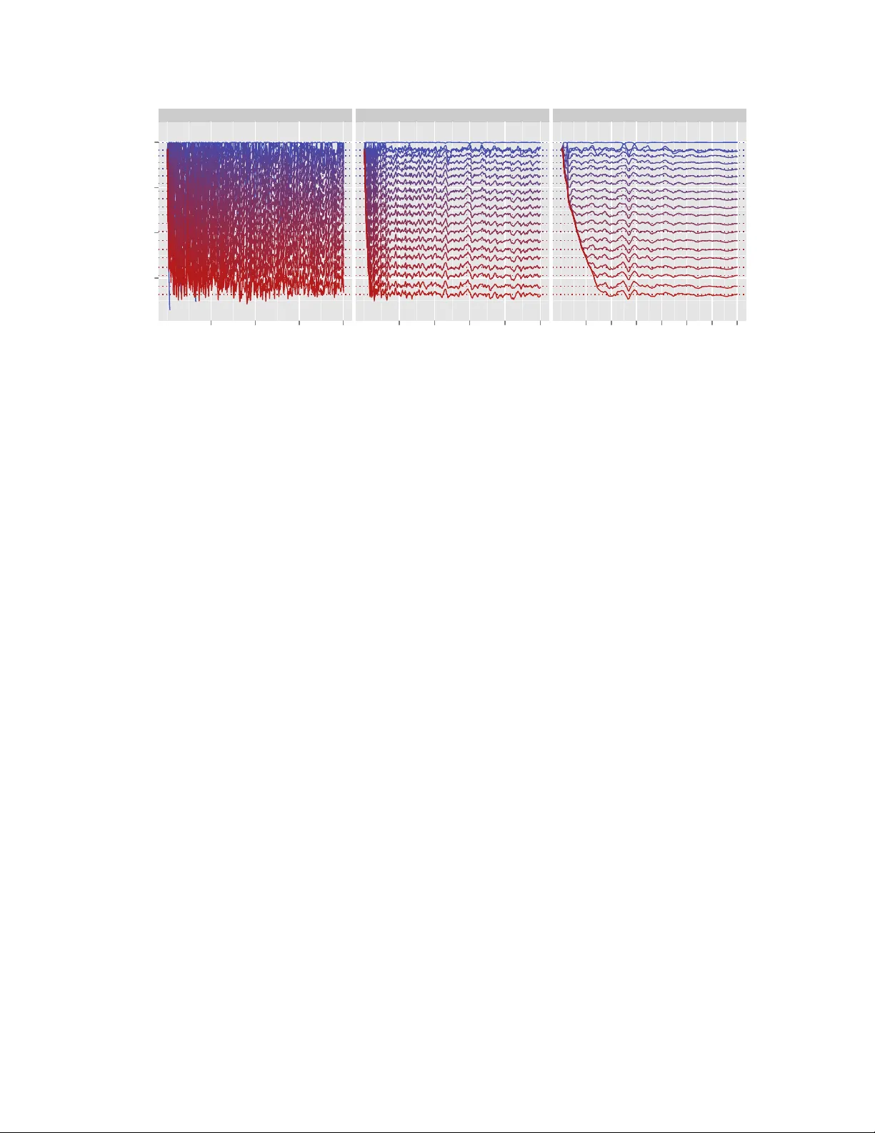
An Adaptiv e In teracting W ang-Landau Algorithm for Automatic Densit y Exploration Luk e Bornn 1 , Pierre E. Jacob 2 , Pierre Del Moral 3 , and Arnaud Doucet 4 1 Departmen t of Statistics, Harv ard Universit y , USA 2 CEREMADE, Universit ´ e Paris-Dauphine, F rance 3 INRIA Bordeaux Sud-Ouest and Universit y of Bordeaux, F rance 4 Departmen t of Statistics, Oxford Univ ersity , UK No vem ber 27, 2024 Abstract While statisticians are w ell-accustomed to p erforming exploratory analysis in the mo deling stage of an analysis, the notion of conducting preliminary general-purp ose exploratory analysis in the Mon te Carlo stage (or more generally , the mo del-fitting stage) of an analysis is an area which w e feel deserv es muc h further attention. T o wards this aim, this pap er prop oses a general-purpose algorithm for automatic density exploration. The proposed exploration algorithm combines and expands up on comp onen ts from v arious adaptiv e Mark ov c hain Mon te Carlo methods, with the W ang-Landau algo- rithm at its heart. Additionally , the algorithm is run on interacting parallel chains – a feature which b oth decreases computational cost as well as stabilizes the algorithm, improving its abilit y to explore the density . P erformance of this new parallel adaptiv e W ang-Landau (P A WL) algorithm is studied in several applications. Through a Bay esian v ariable selection example, the authors demonstrate the con vergence gains obtained with interacting c hains. The ability of the algorithm’s adaptiv e prop osal to induce mo de-jumping is illustrated through a Bay esian mixture mo deling application. Lastly , through a 2D Ising mo del, the authors demonstrate the ability of the algorithm to ov ercome the high correlations encountered in spatial mo dels. The appendices contain the full algorithmic description in pseudo-co de, a tri-mo dal toy example and remarks on the conv ergence of the prop osed algorithm. 1 In tro duction As impro vemen ts in technology introduce measuring devices capable of capturing ever more complex real-w orld phenomena, the accompanying mo dels used to understand such phenomena gro w accordingly . While linear mo dels under the assumption of Gaussian noise were the hallmark of early 20th cen tury 1 statistics, the past several decades ha ve seen an explosion in statistical models which pro duce com- plex and high-dimensional density functions for which simple, analytical in tegration is imp ossible. This gro wth was largely fueled by renewed interest in Bay esian statistics accompanying the Marko v c hain Mon te Carlo (MCMC) revolution in the 1990’s. With the computational p o wer to explore the p osterior distributions arising from Bay esian mo dels, MCMC allow ed practitioners to build mo dels of increasing size and nonlinearit y . As a core comp onen t of man y of the MCMC algorithms discussed later, w e briefly recall the Metrop olis- Hastings algorithm. With the goal of sampling from a density π , the algorithm generates a Marko v chain ( x t ) T t =1 with inv arian t distribution π . F rom a current state x t , a new state x 0 is sampled using a prop osal densit y q η ( x t , x 0 ) parametrized b y η . The prop osed state x 0 is accepted as the new state x t +1 of the c hain with probabilit y min  1 , π ( x 0 ) q η ( x 0 , x t ) π ( x t ) q η ( x t , x 0 )  and if it is rejected, the new state x t +1 is set to the previous state x t . F rom this simple algorithmic description, it is straigh tforward to see that if x t is in a local mo de and the proposal density q η ( x t , x 0 ) has not been carefully chosen to prop ose samples from distant regions, the chain will b ecome stuck in the curren t mode. This is due to the rejection of samples proposed outside the mo de, underscoring the imp ortance of ensuring q η ( x t , x 0 ) is in telligen tly designed. Though standard MCMC algorithms such as the Metrop olis-Hastings algorithm and the Gibbs sam- pler hav e b een studied thoroughly and the conv ergence to the target distribution is ensured under weak assumptions, man y applications in tro duce distributions whic h cannot b e sampled easily b y these algo- rithms. Multiple reasons can lead to failure in practice, ev en if long-run con vergence is guaran teed; the question then b ecomes whether or not the required num b er of iterations to accurately appro ximate the densit y is reasonable giv en the currently a v ailable computational p o wer. Among these reasons, let us cite a few that will be illustrated in later examples: the probability density function migh t b e highly m ultimo dal, in which case the c hain can get stuck in lo cal mo des. Alternatively or additionally , it might b e defined on a high-dimensional state space with strong correlations b et w een the comp onen ts, in which case the prop osal distributions (and in particular their large cov ariance matrices) are v ery difficult to tune man ually . These issues lead to error and bias in the resulting inference, and may b e detected through con vergence monitoring tec hniques (see, e.g., Rob ert and Casella ( 2004 )). Ho wev er, ev en when con ver- gence is monitored, it is possible that en tire modes of the p osterior are missed. T o address these issues, w e turn to a burgeoning class of Mon te Carlo methods which we refer to as “exploratory algorithms.” In the follo wing section, w e discuss the traits that allow exploratory MCMC algorithms to perform inference in m ultimo dal, high-dimensional distributions, connecting these traits to existing exploratory algorithms in the pro cess. In Section 3, we detail one of these, the W ang-Landau algorithm, and prop ose sev eral nov el improv ements that mak e it more adaptive, hence easier to use, and also improv e con vergence. 2 Section 4 applies the prop osed algorithm to v ariable selection, mixture mo deling and spatial imaging, b efore Section 5 concludes. 2 Exploratory Algorithms As emphasized b y Sc hmidler ( 2011 ), there are tw o distinct goals of existing adaptive algorithms. Firstly , algorithms whic h adapt the prop osal according to past samples are largely exploitative, in that they impro ve sampling of features already seen. Ho wev er, mo des or features not y et seen b y the sampler migh t b e quite differen t from the previously explored region, and as suc h adaptation might prev ent adequate exploration of alternate regions of the state space. As an attempted solution to this problem Craiu et al. ( 2009 ) suggest adapting regionally , with parallel chains used to p erform the adaptation. Secondly , there exists a set of adaptive algorithms whose goal is to adapt in suc h a w ay as to encourage density exploration. These include, for instance, the equi-energy sampler ( Kou et al. , 2006 ), parallel tempering ( Sw endsen and W ang , 1986 ; Geyer , 1991 ), and the W ang-Landau ( W ang and Landau , 2001a , b ; Liang , 2005 ; Atc had´ e and Liu , 2010 ) algorithms among others. The algorithm developed here fits into the latter suite of to ols, whose goal is to explore the target density , particularly distan t and p otentially unknown mo des. Although the aforementioned algorithms hav e pro ven efficient for sp ecific c hallenging inference prob- lems, they are not necessarily designed to be generic, and it is often difficult and time-consuming for practitioners to learn and co de these algorithms merely to test a mo del. As such, while statisticians are accustomed to exploratory data analysis, w e b eliev e that there is ro om for generic exploratory Mon te Carlo algorithms to learn the basic features of the distribution or mo del of interest, particularly the lo cations of mo des and regions of high correlation. These generic algorithms would ideally b e able to deal with discrete and con tinuous state spaces and any associated distribution of in terest, and w ould require as few parameters to tune as p ossible, suc h that users can use them before embarking on time- consuming, tailor-made solutions designed to estimate exp ectations with high precision. In this w ay one ma y p erform inference and compare b etw een a wide range of mo dels without building custom-purp ose Mon te Carlo metho ds for each. W e first describe v arious ideas that hav e b een used to explore highly-multimodal densities, and then describ e recen t w orks aimed at automatically tuning algorithmic parameters of MCMC methods, making them able to handle v arious situations without requiring muc h case-sp ecific work from the user. 2.1 Abilit y to Cross Lo w-Density Barriers The fundamen tal problem of density exploration is settling in to lo cal mo des, with an inabilit y to cross lo w-density regions to find alternativ e mo des. F or densities π whic h are highly multi-modal, or “rugged,” one can employ temp ering strategies, sampling instead from a distribution prop ortional to π 1 /τ with temp erature τ > 1. Through temp ering, the p eaks and v alleys of π are smo othed, allo wing easier 3 exploration. This is the fundamental idea b ehind parallel tempering, which employs m ultiple chains at differen t temp eratures; samples are then swapped b et ween c hains, using highly temp ered chains to assist in the exploration of the untempered chain ( Geyer , 1991 ). Marinari and Parisi ( 1992 ) subsequently prop osed simulated tempering, which dynamically mov es a single chain up or do wn the temp erature ladder. One may also fit tempering within a sequential Monte Carlo approac h, whereb y samples are first obtained from a highly temp ered distribution; these samples are transitioned through a sequence of distributions con verging to π using imp ortance sampling and mov es with a Mark ov kernel ( Neal , 2001 ; Del Moral et al. , 2006 ). Ho wev er, using temp ering strategies with complex densities, one must b e careful of phase transitions, where the densit y transforms considerably across a giv en temperature v alue. A related class of algorithms w orks by partitioning the state space along the energy function − log π ( x ). The idea of slicing, or partitioning, along the energy function is the hallmark of several auxiliary v ariable sampling metho ds, whic h iteratively sample U ∼ U [0 , π ( X )] then X ∼ U { X : π ( X ) ≥ U } . This is the fundamen tal idea behind the Sw endsen–W ang algorithm ( Sw endsen and W ang , 1987 ; Edw ards and Sok al , 1988 ) and related algorithms (e.g. Besag and Green ( 1993 ); Higdon ( 1998 ); Neal ( 2003 )). The equi-energy sampler ( Kou et al. , 2006 ; Baragatti et al. , 2012 ), in contrast to the ab o ve auxiliary v ariable metho ds, b egins b y sampling from a highly tempered distribution; once con vergence is reached, a new reduced-temp erature chain is run with up dates from a mixture of Metropolis mov es and exc hanges of the curren t state with the v alue of a previous chain in the same energy band. The process is contin ued un til the temp erature reac hes 1 and the in v arian t distribution of the c hain is the target of interest. As suc h, this algorithm w orks through a sequence of temp ered distributions, using previous distributions to create intelligen t mo de-jumping mov es along an equal-energy set. In a similar vein, the W ang-Landau algorithm ( W ang and Landau , 2001a , b ) also partitions the state space X along a reaction co ordinate ξ ( x ), t ypically the energy function: ξ ( x ) = − log π ( x ), resulting in a partition ( X i ) d i =1 . The algorithm generates a time-inhomogeneous Marko v c hain that admits an in v ariant distribution ˜ π t at iteration t , instead of the target distribution π itself as e.g. in a standard Metrop olis-Hastings algorithm. The distribution ˜ π t is designed such that the generated chain equally visits the v arious regions X i as t → ∞ . Because the W ang-Landau algorithm lies at the heart of our prop osed algorithm, it is extensiv ely described in Section 3 . It is worth discussing a similar, recently proposed algorithm which com bines Marko v chain Monte Carlo and free energy biasing ( Chopin et al. , 2012 ) and its sequen tial Monte Carlo coun terpart ( Chopin and Jacob , 2010 ). The central idea of the latter is to explore a sequence of distributions, successiv ely biasing according to a reaction coordinate ξ in a similar manner. How ever, w e ha ve found the method to b e largely dep endent on selecting a well-c hosen initial distribution π 0 , as is usually the case with sequen tial Monte Carlo metho ds for static inference. If the initial distribution is not c hosen to b e flatter than the target distribution, which is possibly the case since the regions of in terest with resp ect to the target distribution are a priori unkno wn, the efficiency of the SMC metho ds relies mostly on the mo v e steps within the particle filter, whic h are themselv es Metrop olis–Hastings or Gibbs mo ves. 4 2.2 Adaptiv e Prop osal Mechanism Concurren t with the increasing p opularit y of exploratory metho ds, the issue of adaptiv ely fine-tuning MCMC algorithms has also seen considerable gro wth since the foundational pap er of Haario et al. ( 2001 ), including a series of conferences dedicated solely to the problem (namely , Adap’ski 1 through 3 among others); see the reviews of Andrieu and Thoms ( 2008 ) and Atc had´ e et al. ( 2011 ) for more details. While the de-facto standard has historically b een hand-tuning of MCMC algorithms, this new w ork finds in terest in automated tuning, resulting in a new class of methods called adaptive MCMC. The ma jority of the existing literature fo cuses on creating intelligen t prop osal distributions for an MCMC sampler. The principal idea is to exploit past samples to induce b etter mo ves across the state space by matc hing moments of the prop osal and past samples, or b y encouraging a particular acceptance rate of the sampler. The raison d’ˆ etre of these algorithms is that tuning MCMC algorithms by hand is b oth time-consuming and prone to inaccuracies. By automating the selection of the algorithm’s parameters, practitioners migh t sav e considerable time in their analyses. This feature is pivotal in an automated density exploration algorithm. Due to its exploratory nature, it is lik ely that the practitioner migh t not ha ve complete kno wledge of ev en the scale of the densit y support; as a result, having a prop osal distribution which adapts to the densit y at hand is a crucial step in the automation process. One must be careful in selecting the type of adaptation mec hanism emplo yed to encourage exploration, rather th an simply exploiting previously explored modes. F or instance, tuning a prop osal co v ariance to a previously visited mo de migh t preven t the algorithm from reaching as yet unexplored modes in the direction of the current mo de’s minor axis. Additionally , when com bined with a progressiv ely biased distribution as in the W ang-Landau algorithm, it is desirable to ha ve a prop osal whic h first samples what it sees w ell, then later grows in step size to b etter explore the flattened (biased) distribution. 3 Prop osed Algorithm W e now develop our prop osed algorithm. After recalling the W ang-Landau algorithm, which constitutes the core of our metho d, we describ e three improv ements: an adaptiv e binning strategy to automate the difficult task of partitioning the state space, the use of interacting parallel chains to improv e the con ver- gence sp eed and use of computational resources, and finally the use of adaptive prop osal distributions to encourage exploration as w ell as to reduce the n um b er of algorithmic parameters. W e detail at the end of the section ho w to use the output of the algorithm, which we term parallel adaptive W ang-Landau (P A WL) to answ er the statistical problem at hand. 3.1 The W ang-Landau Algorithm As previously mentioned, the W ang-Landau algorithm generates a time-inhomogeneous Marko v chain that admits a distribution ˜ π t as the inv arian t distribution at iteration t . The biased distribution ˜ π t 5 targeted b y the algorithm at iteration t is based on the target distribution π , and mo dified suc h that a) the generated chain visits all the sets ( X i ) d i =1 equally , that is the proportion of visits in each set is con verging to d − 1 when t go es to infinity; and b) the restriction of the modified distribution ˜ π t to eac h set X i coincides with the restriction of the target distribution π to this set, up to a m ultiplicative constan t. The mo dification (a) is crucial, as inducing uniform exploration of the sets is the biasing mechanism whic h improv es exploration; in fact similar strategies are used in other fields, including com binatorial optimization ( W ei et al. , 2004 ). Ideally the biased distribution ˜ π w ould not dep end on t , and w ould be a v ailable analytically as: ˜ π ( x ) = π ( x ) × 1 d d X i =1 I X i ( x ) ψ ( i ) (1) where ψ ( i ) = R X i π ( x )d x and I X i ( x ) is equal to 1 if x ∈ X i and 0 otherwise. Chec king that using ˜ π as the in v ariant distribution of a MCMC algorithm would v alidate p oin ts a) and b) is straigh tforward. Figure 1 illustrates a univ ariate target distribution π and its corresp onding biased distribution ˜ π under t wo different partitions of the state space. X Log Density −12 −10 −8 −6 −4 −2 0 Original Density , with partition lines −5 0 5 10 15 Biased by X −5 0 5 10 15 Biased by Log Density −5 0 5 10 15 Figure 1: Probabilit y density functions for a univ ariate distribution π and its biased version ˜ π when partitioning the state space along the x -axis ( ξ ( x ) = x , middle) and the log density ( ξ ( x ) = − log π ( x ), righ t). The left-most plot also shows the partitioning of the state space with ξ ( x ); in b oth cases d = 20. The biasing is done suc h that the in tegral R X i ˜ π ( x )d x is the same for all X i (areas under the curve for eac h set) and such that π and ˜ π coincide on eac h set X i , up to a multiplicativ e constant. In practical situations, ho wev er, the in tegrals ( ψ ( i )) d i =1 are not a v ailable, hence we wish to plug estimates ( θ ( i )) d i =1 of ( ψ ( i )) d i =1 in to Equation ( 1 ). The W ang-Landau algorithm is an iterative algorithm whic h join tly generates a sequence of estimates ( θ t ( i )) t for all i and a Marko v c hain ( X t ) t , suc h that when t go es to infinit y , θ t ( i ) con verges to ψ ( i ) and consequently , the distribution of X t con verges to ˜ π . W e denote by ˜ π θ t the biased distribution obtained by replacing ψ ( i ) by its estimate θ t ( i ) in Equation ( 1 ). Note that the normalizing constan t of ˜ π θ t is no w unkno wn. A simplified version of the W ang-Landau algorithm is giv en in Algorithm 1 . 6 Algorithm 1 Simplified W ang-Landau Algorithm 1: P artition the state space in to d regions {X 1 , . . . , X d } along a reaction co ordinate ξ ( x ). 2: First, ∀ i ∈ { 1 , . . . , d } set θ ( i ) ← 1. 3: Choose a decreasing sequence { γ t } , typically γ t = 1 /t . 4: Sample X 0 from an initial distribution π 0 . 5: for t = 1 to T do 6: Sample X t from P θ t − 1 ( X t − 1 , · ), a transition k ernel with in v ariant distribution ˜ π θ t − 1 ( x ). 7: Up date the bias: log θ t ( i ) ← log θ t − 1 ( i ) + γ t ( I X i ( X t ) − d − 1 ). 8: Normalize the bias: θ t ( i ) ← θ t ( i ) / P d i =1 θ t ( i ). 9: end for The rationale b ehind the update of the bias is that if the c hain is in the set X i , the probability of remaining in X i should b e reduced compared to the other sets through an increase in the asso ciated bias θ t ( i ). Therefore the chain is pushed to wards the sets that hav e b een visited less during the previous iterations, improving the exploration of the state space so long as the partition ( X i ) d i =1 is well c hosen. While this biasing mechanism adds cost to each iteration of the algorithm the tradeoff is improv ed exploration. In step 6, the transition k ernel is t ypically a Metrop olis-Hastings mov e, due to the lack of conjugacy brought ab out by biasing. In this simplified form the W ang-Landau algorithm reduces to standard sto c hastic approximation, where the term γ t decreases at each iteration. The algorithm as given in W ang and Landau ( 2001a , b ) uses a more sophisticated learning rate γ t whic h do es not decrease deterministically , but instead only when a certain criterion is met. This criterion, referred to as the “flat histogram” criterion, is met when for all i ∈ { 1 , . . . , d } , ν ( i ) is close enough to d − 1 , where w e denote b y ν ( i ) the proportion of visits of ( X t ) in the set X i since the last time the criterion was met. Hence we in tro duce a real n umber c to con trol the distance b etw een ν ( i ) and d − 1 , and an integer k to count the num b er of criteria already met. W e describ e the generalized W ang-Landau in Algorithm 2 . Algorithm 2 W ang-Landau Algorithm 1: P artition the state space in to d regions {X 1 , . . . , X d } along a reaction co ordinate ξ ( x ). 2: First, ∀ i ∈ { 1 , . . . , d } set θ ( i ) ← 1 , ν ( i ) ← 0. 3: Choose a decreasing sequence { γ k } , typically γ k = 1 /k . 4: Sample X 0 from an initial distribution π 0 . 5: for t = 1 to T do 6: Sample X t from P θ t − 1 ( X t − 1 , · ), a transition k ernel with in v ariant distribution ˜ π θ t − 1 ( x ). 7: Up date the prop ortions: ∀ i ∈ { 1 , . . . , d } ν ( i ) ← 1 t [( t − 1) ν ( i ) + I X i ( X t )]. 8: if “flat histogram”: max i ∈ [1 ,d ] | ν ( i ) − d − 1 | < c/d then 9: Set k ← k + 1. 10: Reset ∀ i ∈ { 1 , . . . , d } ν ( i ) ← 0. 11: end if 12: Up date the bias: log θ t ( i ) ← log θ t − 1 ( i ) + γ k ( I X i ( X t ) − d − 1 ). 13: Normalize the bias: θ t ( i ) ← θ t ( i ) / P d i =1 θ t ( i ). 14: end for When c is set to low v alues (e.g. c = 0 . 1 or 0 . 5), the algorithm must explore the v arious regions suc h that the frequency of visits to the region X i is approximately d − 1 b efore the learning rate γ k is 7 decreased. Also, the algorithm ma y b e further generalized to target a desired frequency φ i instead of the same frequency d − 1 for every set; while such strategies may b e useful, as demonstrated in the following section, for notational simplicity we fo cus on the case φ i = d − 1 . As already mentioned, to answ er the general question of exploring the support of a target density π , the default choice for the reaction co ordinate is the energy function: ξ ( x ) = − log π ( x ), which has the benefit of being one-dimensional regardless of the dimension of the state space X . How ever, for specific mo dels other reaction coordinates ha ve b een used, such as one (or more) of the comp onen ts x j of x or a linear combination of comp onen ts of x . In the applications in Section 4 we discuss the use of alternative reaction co ordinates further. W e no w prop ose improv ements to the W ang-Landau algorithm to increase its flexibilit y and efficiency . 3.2 A No vel Adaptiv e Binning Strategy The W ang-Landau and equi-energy sampler algorithms are known to p erform w ell if the bins, or partitions of the one-dimensional reaction co ordinate ξ ( x ), are w ell chosen. How ever, dep ending on the problem it migh t be difficult to choose the bins to optimize sampler p erformance. A t ypical empirical approach to deal with this issue is to first run, for example, an adaptive MCMC algorithm to find at least one mo de of the target distribution. The generated sample and the asso ciated target density ev aluations determine a first range of the target densit y v alues whic h can be used to initialize the bins. A t this p oin t the user can choose a wider range of target densit y v alues (e.g. by m ultiplying the range by 2), in order to allo w for a wider exploration of the space. Within this initial range, one must still decide the num b er of bins. Due to difficulties with selecting the bins, it has been suggested that one should adaptiv ely compare adjacen t bins, splitting a bin if the corresponding estimate θ is significantly larger than a neigh b oring v alue ( Sc hmidler , 2011 ). Because each ψ i is a given bin’s normalizing constant, we feel it is more important to main tain uniformit y within a bin to allow easy within-bin mo vemen t. Our prop osed approach to ac hieve this “flatness” is to lo ok at the distribution of the realized reaction co ordinate v alues within eac h bin. Figure 2 illustrates this distribution on an artificial histogram. The plot of Figure 2(a) shows a situation where, within one bin, the distribution might b e strongly sk ewed tow ards one side. In this artificial example, v ery few p oints hav e visited the left side of the bin, which suggests that moving from this bin to the left neigh b oring bin migh t b e difficult. W e prop ose to consider the ratio of the num b er of p oin ts on the left side of the middle (dashed line) o ver the num b er of points within the bin as a very simple proxy for the discrepancy of the c hains within one bin (see e.g. Niederreiter ( 1992 ) for muc h more sophisticated discrepancy measures). In a broad outline, if this ratio was around 50%, the within-bin histogram would b e roughly uniform. On the con trary , the ratio corresp onding to Figure 2(a) is around 7%. Our strategy is to split the bin if this ratio go es b elo w a giv en th reshold, sa y 25%; t wo new bins are created, corresp onding to the left side and the righ t side of the former bin, and each bin is assigned a w eight of θ / 2 where θ is the weigh t of the former bin. These pro vide starting v alues for the e stimation of the w eight of the new bins during the following iterations of the algorithm. Note also that the desired frequency of visits to each of the new bins, which 8 Log density Frequency (a) Unique bin b efore the split Log density Frequency (b) Two bins after the split Figure 2: Artificial histograms of the log target densit y v alues asso ciated to the chains generated b y the algorithm, within a single bin (left) and within t wo bins created b y splitting the former bin (righ t). w as for instance equal to 1 /d before the split, has to be sp ecified as well. In the numerical exp erimen ts, w e set the desired frequency of the new bins as one half of the desired frequency of the former bin. Figure 2(b) shows the distribution of samples within the tw o new bins. The resulting histogram is not uniform, y et exhibits a more even distribution within the bin – a feature which is exp ected to help the c hain to mo ve from this bin to the left neigh b oring bin. The threshold could b e set closer to 50%, which would result in more splits and therefore more bins. In practice it is not necessary to chec k whether the bins hav e to b e split at ev ery iteration. Our strategy is to c heck ev ery n -th iteration, until the flat histogram criterion is met for the first time. When it is met, it means that the c hains can mo ve easily b et ween the bins, and hence the bins can b e kept unc hanged for the remaining iterations. Finally , when implementing the automatic binning strategy for discrete distributions, one m ust ensure that a new bin corresp onds to actual p oin ts in the state space. F or example if the bins are along the energy v alues and the state space is finite, there are certainly in terv als of energy to whic h no states corresp onds, and that would therefore nev er b e reac hed. Section 4 demonstrates the prop osed adaptiv e binning strategy in practice. In addition to allo wing for splitting of bins, it is also imp ortan t to allow the range of bins to extend if new states are found outside of the particular range. That said, one must differen tiate betw een the t wo extremes of the reaction co ordinate. F or example, if ξ ( x ) = − log π ( x ), then one migh t not wish to add more low-densit y (high-energy) bins, whic h would induce the sampler to explore further and further into the tails. Ho wev er, if one finds a new high-densit y (lo w-energy) mode b ey ond the energy range previously seen, then the sampler might b ecome stuck in this new mo de. In this case, w e prop ose to extend the first bin corresp onding to the low est level of energy to alw ays include the low est observ ed v alues. The 9 adaptiv e partition ( X i,t ) d t i =1 of the state space takes the following form at time t : X 1 ,t = [ e min ,t , e 1 ,t ] , X 2 ,t = [ e 1 ,t , e 2 ,t ] , . . . X d t ,t = [ e d t − 1 ,t , + ∞ ) where e min ,t = min t ≥ 0 {− log π ( X t ) } and ( e 1 ,t , . . . , e d t − 1 ,t ) defines the limits of the inner bins at time t , whic h is the result of initial bin limits ( e 1 , 0 , . . . , e d 0 − 1 , 0 ), an d possible splits b et ween time 0 and time t . As suc h, if new lo w-energy v alues are found, the bin X 1 ,t is widened. If this results in unequal exploration across the reaction co ordinate, then the adaptiv e bin-splitting mec hanism will automatically split this newly widened bin. 3.3 P arallel Interacting Chains W e prop ose to generate multiple chains instead of a single one to improv e computational scalability through parallelization as w ell a s particle div ersity . The use of interacting chains has b ecome of muc h in terest in recen t y ears, with the multiple c hains used to create div erse proposals ( Casarin et al. , 2011 ), to induce long-range equi-energy jumps ( Kou et al. , 2006 ), and to generally impro v e sampler p erformance; see Atc had´ e et al. ( 2011 ), Bro c kwell et al. ( 2010 ), and Byrd ( 2010 ) for recen t dev elopments. The use of parallelization is not constrained to multiple c hains, how ev er, and has also been employ ed to sp eed up the generation of a single c hain through pre-fetc hing ( Bro c kwell , 2006 ). Let N b e the desired n umber of chains. W e follow Algorithm 2 , with the following mo difications. First we generate N starting points X 0 = ( X (1) 0 , . . . , X ( N ) 0 ) indep enden tly from an initial distribution π 0 (Algorithm 2 line 4 ). Then at iteration t , instead of mo ving one c hain using the transition k ernel P θ t − 1 , w e mo ve the N c hains using the same transition k ernel, asso ciated with the same bias θ t − 1 (Algorithm 2 line 6 ). W e emphasize that the bias θ is common to all chains, which mak es the proposed metho d differen t from running W ang-Landau c hains entirely in parallel. The prop ortions ν ( i ) are up dated using all the c hains, simply by replacing the indicator function I X i ( X t ) b y the mean N − 1 P N j =1 I X i ( X ( j ) t ), that is the prop ortion of chains curren tly in set X i (Algorithm 2 line 7 ). Likewise the up date of the bias uses all the c hains, again replacing the indicator function by the prop ortion of chains currently in a given set (Algorithm 2 line 12 ). W e hav e therefore replaced indicator functions in the W ang-Landau algorithm by the la w of the MCMC c hain associated with the curren t parameter. Since this law is not accessible, we p erform a mean field approximation at eac h time step. A similar expression has recently b een employ ed b y Liang and W u ( 2011 ) for use in parallelizing the sto chastic appro ximation Monte Carlo algorithm ( Liang et al. , 2007 ; Liang , 2009 ). Note that while w e hav e designed the chains to communicate at eac h iteration, such frequent message passing can b e costly , particularly on graphics pro cessing units. In suc h situations, one could alter the algorithm suc h that the chains only communicate p eriodically . Our results (see Section 4 ) show that N in teracting c hains run for T iterations can strongly outp erform a single chain run for N × T iterations, in terms of v ariance of the resulting estimates. Sp ecifically , having a sample appro ximately distributed according to π θ t ( x ) instead of a single p oin t at iteration t impro v es 10 and stabilizes the subsequent estimate θ t +1 . W e explore the tradeoff b et ween N and T in more detail in Section 4 . Note that, while the original single-chain W ang-Landau algorithm was not straigh tforw ard to paral- lelize due to its iterative nature, the prop osed algorithm can strongly b enefit from multiple processing units: at a giv en iteration the N mov e steps can b e done in parallel, as long as the results are consequen tly collected to up date the bias b efore the next iteration. Therefore if multiple pro cessors are a v ailable, as e.g. in recent ce n tral processing units and in graphics processing units (see e.g. Lee et al. ( 2010 ); Suc hard and Ram baut ( 2009 )), the computational cost can b e reduced m uch more than what w as possible with the single-chain W ang-Landau algorithm. T o summarize, the proposed use of interacting c hains can b oth improv e the con vergence of the estimates, regardless of the num b er of av ailable pro cessors, and additionally b enefit from m ultiple pro cessors. Finally , an additional b enefit of using N parallel chains is that they can start from v arious points, dra wn from the initial distribution π 0 ; hence if π 0 is flat enough, the c hains can start from different lo cal mo des, which improv es de facto the exploration. Ho wev er, we show in Section 4 that the c hains still explore the space even if they start within the same mo de, and hence the efficiency of the method do es not rely on the c hoice of π 0 , con trary to what w e observ ed with sequen tial Mon te Carlo methods. Additionally , b ecause the sampler is attempting to explore both the state-space as w ell as the range of the reaction co ordinate sim ultaneously , our parallel form ulation allows the sampler to b orro w strength b et w een c hains, pro viding for exploration of the reaction co ordinate without ha ving to mov e a single c hain across p oten tially large and high-dimensional state-spaces to trav erse the reaction co ordinate v alues. 3.4 Adaptiv e Prop osal Mechanism As discussed earlier, it is important to automate the proposal mechanism to improv e mov emen t across the state space. A well-studied proxy for optimal mo vemen t is the algorithm’s Metrop olis-Hastings acceptance rate. T o o lo w an acceptance rate signifies the algorithm is attempting to make mo ves that are to o large, and are therefore rejected. T o o high an acceptance rate signifies the algorithm is barely mo ving. As suc h, we suggest adaptively tuning the prop osal v ariance to encourage an acceptance rate of 0 . 234 as recommended in Roberts et al. ( 1997 ), although we ha ve found settings in the range 0 . 1 to 0 . 5 to w ork w ell in all examples tested. The Robbins-Monro sto c hastic appro ximation update of the proposal standard deviation σ t is as follo ws: σ t +1 = σ t + ρ t (2 I ( A > 0 . 234) − 1) (2) where t is the current iteration of the algorithm, ρ t is a decreasing sequence (typically ρ t = 1 /t ), and A is the acceptance rate (prop ortion of accepted mo ves) of the particles. Through this up date, the prop osal v ariance grows after samples are accepted, and shrinks when samples are rejected, encouraging exploration of the state space. 11 Another approach to adaptively tuning the prop osal distribution is to use the following mixture of Gaussian random-walks: X ∗ ∼ w 1 N  X t − 1 , (2 . 38) 2 p Σ t  + w 2 N  X t − 1 , ( σ I ) 2 p I p  (3) with w 1 + w 2 = 1, Σ t the empirical cov ariance of the c hain history – an estimator of the co v ariance structure of the target – and I p the p × p iden tity matrix where p is the dimension of the target space. The first comp onen t of this mixture mak es the prop osal adaptive and able to learn from the past, while the second component helps to explore the space. F or instance, if the c hain is stuck in a mode, the first comp onen t’s v ariance migh t become small, yet the second comp onent guarantees a c hance to even tually escap e the mo de. Hence the second component acts as a “safety net” and therefore its weigh t is small, t ypically w 2 = 0 . 05, and its standard deviation σ I ma y b e set large to improv e mixing ( Guan and Krone , 2007 ). In our con text where parallel chains are run together, w e use all the chains to estimate the empirical co v ariance Σ t at eac h iteration. Note that the computation of this cov ariance do es not require the storage of the whole history of the c hain and can b e done at constant cost, since recurrence formulae exist to compute the empirical co v ariance, as explained for instance in W elford ( 1962 ). The v alue 2 . 38 2 is justified by asymptotic optimalit y reflections on certain classes of mo dels (see, e.g., Roberts et al. ( 1997 ) and Rob erts and Rosen thal ( 2009 )). 3.5 Using the Output to P erform Inference While the resulting samples from the proposed algorithm P A WL are not from π , but rather an appro xi- mation of the biased v ersion ( 1 ), one can use importance sampling or adv anced sequen tial Mon te Carlo ideas to transition the samples to π (see Chopin and Jacob ( 2010 ) for details). Alternativ ely , the samples from the exploratory algorithm can b e used to seed a more traditional MCMC algorithm, as adv o cated b y Sc hmidler ( 2011 ). The pseudo-co de for P A WL, combining the parallel W ang-Landau algorithm with adaptive binning and proposal mechanisms, is giv en in the Appendix. Before pro ceeding to examples, it is imp ortan t to reiterate the importance of the v alues ψ ( i ) = R X i π ( x )d x . Sp ecifically , certain c hoices of the reaction co ordinate ξ ( x ) result in ψ ( i ) ha ving inherent v alue. F or example, it is possible in a mo del selection application to use the mo del order as ξ ( x ), in which case the v alues ψ ( i ) could b e emplo yed to calculate Ba yes factors and other quantities of in terest. 4 Applications W e no w demonstrate P A WL applied to three examples including v ariable selection, mixture mo deling, and spatial imaging. A fourth pedagogical example is av ailable in the app endices. In each application 12 w e w alk through our prop osed algorithm (describ ed explicitly as Algorithm 3 in the Appendix), first running preliminary (adaptive) Metropolis-Hastings MCMC to determine the initial range for the reaction co ordinate ξ and initial v alues for the proposal parameters and starting state of the interacting W ang- Landau chains. This range is then increased to encourage exploration of low-densit y regions of the space, and an initial num b er of bins is sp ecified. Once this groundw ork is set, the same Metropolis-Hastings algorithm run in the preliminary stage is embedded within the P A WL algorithm. 4.1 g -Prior V ariable Selection W e pro ceed by conducting v ariable selection on the p ollution data set of McDonald and Sch wing ( 1973 ), wherein mortality is related to pollution levels through 15 indep endent v ariables including mean annual precipitation, p opulation p er household, and av erage annual relativ e humidit y . Measured across 60 metrop olitan areas, the resp onse v ariable y is the age-adjusted mortality rate in the giv en metrop olitan area. Our goal is to identify the pollution-related indep enden t v ariables which b est predict the resp onse. With 15 v ariables, calculating the posterior probabilities of the 32 , 768 mo dels exactly is p ossible but time-consuming. W e hav e chosen this size of data set to pro vide for difficult p osterior exploration, yet allo w a study of con v ergence of θ to wards ψ . With an ey e to wards model selection, we introduce the binary indicator v ariable γ ∈ { 0 , 1 } p , where γ j = 1 means the v ariable x j is included in the mo del. As such, γ can describ e all of the 2 p p ossible mo dels. Consider the normal likelihoo d y | µ, X , β , σ 2 ∼ N n ( X β , σ 2 I n ) . (5) If X γ is the mo del matrix whic h excludes all x j ’s if γ j = 0, we can emplo y the following prior distributions for β and σ 2 ( Zellner , 1986 ; Marin and Rob ert , 2007 ): π ( β γ , σ 2 | γ ) ∝ ( σ 2 ) − ( q γ +1) / 2 − 1 exp  − 1 2 g σ 2 β T γ ( X T γ X γ ) β γ  . where q γ = 1 T n γ represents the n umber of v ariables in the mo del. While selecting g can b e a difficult problem, we hav e chosen it to b e very large ( g = exp(20)) to induce a sparse mo del, which is difficult to explore due to the small marginal probabilities of most v ariables. After in tegrating ov er the regression co efficien ts β , the posterior densit y for γ is thus π ( γ | y , X ) ∝ ( g + 1) − ( q γ +1) / 2  y T y − g g + 1 y T X γ ( X T γ X γ ) − 1 X γ y  − n/ 2 . (6) While w e select the log energy function − log π ( x ) as the reaction co ordinate ξ ( x ) for our analysis, it is w orth noting that many other options exist. F or instance, it would b e natural to consider the model saturation q γ /p , which w ould ensure exploration across the differen t mo del sizes. Ho w ever, w e select 13 Iteration Log( θ ) −60 −40 −20 0 N = 1 20000 40000 60000 80000 N = 10 5000 10000 15000 20000 25000 N = 100 500 1000 1500 2000 2500 3000 3500 Figure 3: V ariable selection example: conv ergence of W ang-Landau for N = 1 , 10 , 100. Iterations set suc h that each algorithm runs in 2 minutes ( ± 5 seconds). θ for each bin sho wn in solid lines. T rue v alues ( ψ ) shown as dotted lines. ξ ( x ) = − log π ( x ) to emphasize the universalit y of using the energy function as the reaction coordinate. W e first run a preliminary Metrop olis-Hastings algorithm which flips a v ariable on/off at random, accepting or rejecting the flip based on the resulting p osterior densities. Due to high correlation b etw een v ariables, a b etter strategy migh t b e to flip m ultiple v ariables at once; ho wev er, w e restrain from exploring this to demonstrate P A WL’s abilit y to mak e viable ev en po orly designed Metropolis-Hastings algorithms. The preliminary algorithm run found v alues 377 < − log π ( x ) < 410, whic h we extend sligh tly to create 20 equally spaced bins in the range [377 , 450]. It is w orth reiterating that the resulting samples generated from P A WL are from a biased v ersion of π ; as such, imp ortance sampling tec hniques could be used to reco ver π , or the samples obtained could be used to seed a more traditional MCMC algorithm. Due to the size of the problem, we are able to en umerate all p osterior v alues, and hence ma y calcu- late ψ exactly . As suc h, we begin b y examining the effect of the n umber of particles N on the parallel W ang-Landau algorithm. T o further focus on this aspect, we suppress adaptive binning and proposals for this example. Figure 3 shows the con vergence of θ to Ψ for N = 1 , 10 , 100. W e see that the algorithm’s con vergence improv es with more particles. Using N = 100 particles, w e no w examine P A WL compared to the Metropolis-Hastings algorithm (run on N chains) men tioned ab o v e on the unnormalized targets π , π 1 / 10 , π 1 / 100 . Consider Figure 4 ; on the target distribution π , the Metrop olis-Hastings algorithm b e- comes stuck in high-probability regions. How ev er, on the temp ered distributions, the algorithm explores the space more thoroughly , although not to the same level as P A WL. Sp ecifically , P A WL explores a m uch wider range of mo dels, including the highest probability mo dels, whereas the temp ered distributions do not. Here the W ang-Landau algorithm as well as the Metropolis-Hastings algorithm both use N = 100 c hains for T = 3500 iterations, the former taking 253 ± 13 seconds and the latter taking 247 ± 15 seconds across 10 runs, indicating that the additional cost for P A WL is negligible. 14 Iteration Model Saturation 0.0 0.1 0.2 0.3 0.4 0.5 0.6 0.7 0.0 0.1 0.2 0.3 0.4 0.5 0.6 0.7 W ang−Landau Metropolis−Hastings, T emp = 10 500 1000 1500 2000 2500 3000 3500 Metropolis−Hastings, T emp = 1 Metropolis−Hastings, T emp = 100 500 1000 1500 2000 2500 3000 3500 Figure 4: V ariable selection example: exploration of model space b y P A WL and Metropolis-Hastings at 3 temp erature settings. (a) Mo del Saturation (proportion of non-zero v ariables in model) as function of algorithm iterations. The solid lines are the mean of N = 100 c hains, while the shaded regions are the middle 95% of the chains. 15 4.2 Mixture Mo deling Mixture models pro vide a challenging case of m ultimo dality , due partly to the complexit y of the mo del and partly to a phenomenon called “lab el switching” (see e.g. F r ¨ uhwirth-Sc hnatter ( 2006 ) for a bo ok co vering Ba yesian inference for these mo dels, Dieb olt and Rob ert ( 1994 ) and Ric hardson and Green ( 1997 ) for seminal pap ers using MCMC for mixture mo dels, and Stephens ( 2000 ) and Jasra et al. ( 2005 ) on the label switc hing problem). Articles describing explorativ e MCMC algorithms often tak e these mo dels as b enc hmarks, as e.g. population MCMC and SMC metho ds in Jasra et al. ( 2007 ), the W ang- Landau algorithm in Atc had ´ e and Liu ( 2010 ), free energy metho ds in Chopin et al. ( 2012 ); Chopin and Jacob ( 2010 ), and parallel temp ering with equi-energy mo ves in Baragatti et al. ( 2012 ). Consider a Ba y esian Gaussian mixture mo del, i.e. for i = 1 , . . . n , p ( y i | q , µ, λ ) = K X k =1 q k ϕ ( y i ; µ k , λ − 1 k ) , where ϕ is the probabilit y density function of the Gaussian distribution, K is the n umber of comp onents, q k , µ k and λ k are resp ectively the weigh t, the mean and the precision of component k . The component index k is also called its lab el. F ollowing Ric hardson and Green ( 1997 ), the prior is tak en as, for k = 1 , . . . , K , µ k ∼ N( M , κ − 1 ) , λ k ∼ Gamma( α, β ) , β ∼ Gamma( g , h ) , ( q 1 , . . . , q K − 1 ) ∼ Diric hlet K (1 , . . . , 1) with, e.g., κ = 4 /R 2 , α = 2, g = 0 . 2, h = 100 g /αR 2 , M = ¯ y , R =range( y ). The in v ariance of the likelihoo d to p erm utations in the labelling of the components leads to the “label switc hing” problem: since there are K ! possible permutations of the lab els, each mode has necessarily K ! − 1 replicates. W e emphasize that this mo del has b een thoroughly studied and is hence w ell-understo o d from a modeling p oin t of view, but it still induces a computationally c hallenging sampling problem for whic h difficult y can be artificially increased through the num b er of components K . Note that in this parametrization β , the rate of the Gamma prior distribution of the precisions λ k , is estimated along with the parameters of interest q 1: K − 1 , µ 1: K and λ 1: K . Chopin et al. ( 2012 ); Chopin and Jacob ( 2010 ) suggest that β can be used as a reaction coordinate, since a large v alue of β results in a small precision and hence in a flatter posterior distribution of the other parameters, which is easier to explore than the distribution associated with smaller v alues of β ; we refer to these articles for further exploration of this c hoice of reaction co ordinate, and instead default to ξ ( x ) = − log π ( x ). W e create a synthetic 100-sample from a Gaussian mixture with k = 4 comp onents, w eights 1 / 4, means − 3, 0, 3, 6 and v ariances 0 . 55 2 as in Jasra et al. ( 2005 ). The goal is to explore the highly m ultimo dal p osterior distribution of the 13-dimensional parameter θ = ( w 1:4 , µ 1:4 , λ 1:4 , β ) where w k is the unnormalized weigh t: q k = w k / P K k =1 w k . Unnormalized w eights may b e handled straightforw ardly 16 in MCMC algorithms since they are defined on R + and not on the K -simplex as with the q k . The prop osed algorithm is compared to a Sequen tial Monte Carlo sampler (SMC) and a parallel adaptiv e Metrop olis–Hastings (P AMH) algorithm, that w e detail b elo w. W e admittedly use naive v ersions of these comp etitors, arguing that most improv emen ts of these could b e carried o ver to P A WL. F or instance, a mixture of Mark ov k ernels as suggested for the SMC algorithm in Section 3.2 of Jasra et al. ( 2007 ) can b e used in the prop osal distribution of P A WL; and since P A WL is a p opulation MCMC algorithm, exc hange and crosso ver mov es could b e used as well, as suggested for the P opulation SAMC algorithm in Liang and W u ( 2011 ). T o get a plausible range of v alues for the reaction co ordinate of the prop osed algorithm without user input, an initial adaptiv e MCMC algorithm is run with N = 10 c hains and T init = 1 , 000 iterations. The initial points of these chains are dra wn from the prior distribution of the parameters. This provides a range of log density v alues, from whic h w e compute the 10% and 90% empirical quantiles, denoted b y q 10 and q 90 resp ectiv ely . In a conserv ative spirit, the bins are c hosen to equally divide the in terv al [ q 10 , q 10 + 2( q 90 − q 10 )] in 20 subsets. Hence the algorithm is going to explore log densit y v alues in a range that is appro ximately twice as large as the v alues initially explored. Note that we use quantiles instead of minim um and maxim um v alues to mak e the method more robust. Next, P A WL itself is run for T = 200 , 000 iterations, starting from the terminal p oin ts of the N preliminary chains, resulting in a total num b er of N ( T + T init ) target densit y ev aluations. In this situation, even with only 100 data p oin ts, most of the computational cost go es in to the ev aluation of the target density . This confirms that algorithmic parameters such as the n umber of bins do es not significan tly affect the ov erall computational cost, at least as long as the target densit y is not extremely c heap to ev aluate. The adaptive prop osal is such that it targets an acceptance rate of 23 . 4%. Meanwhile the P AMH algorithm using the same adaptive prop osal is run with N = 10 c hains and T ? = 250 , 000 iterations, hence relying on more target densit y ev aluations for a comparable computational cost. Finally , the SMC algorithm is run on a sequence of temp ered distribution ( π k ) K k =1 , each densit y b eing defined by: π k ( x ) ∝ π ζ k ( x ) p 1 − ζ k 0 ( x ) where p 0 is an initial distribution (here tak en to b e the prior distribution), and ζ k = k /K . The n um b er of steps K is set to 100 and the num b er of particles to 40 , 000. When the Effectiv e Sample Size (ESS) go es b elo w 90%, we p erform a systematic resampling and 5 consecutive Metropolis–Hastings mov es. W e use a random walk prop osal distribution, which v ariance is tak en to b e c ˆ Σ where ˆ Σ is the empirical cov ariance of the particles and c is set to 10%; see Jasra et al. ( 2007 ) for more details. The parameters are chosen to induce a computational cost comparable to the other metho ds. Ho wev er for the SMC sampler the n umber of target densit y ev aluations is a random num b er, since it dep ends on the random n umber of resampling steps: the computational cost is in general less predictable than using MCMC. First we lo ok at graphical represen tations of the generated samples. Figure 5 shows the resulting p oin ts pro jected on the ( µ 1 , µ 2 ) plane, restricted on [ − 5 , 9] 2 . In this plane there are 12 replicates of each 17 mo de, indicated by target sym b ols in Figure 5(a) . These pro jections do not allow one to chec k that all the mo des were visited since they pro ject the 13-dimensional target space on a 2-dimensional space. Figure 5(b) shows that the adaptiv e MCMC metho d clearly misses some of the modes, while visiting man y others. Figure 5(c) sho ws how the chains generated b y the modified W ang-Landau algorithm easily explore the space of in terest, visiting b oth global and local mo des. T o reco ver the main mo des from these c hains, w e use the final v alue of the bias, θ T , as imp ortance w eights to correct for the bias induced b y the algorithm; in Figure 5(c) the importance weigh ts define the transparency of eac h p oin t: the darker the p oin t, the more w eight it has. Finally Figure 5(d) sho ws ho w the SMC sampler also put particles in eac h mode; again the transparency of the points is prop ortional to their weigh ts. W e now turn to m ore quantitativ e measures of the error made on marginal quantities. Since the comp onen t means admit 4 identical mo des around − 3, 0, 3 and 6, w e kno w that their ov erall mean is appro ximately equal to µ ? = 1 . 5. W e then compute the follo wing error measuremen t: error = v u u t K X k =1 ( ˆ µ k − µ ? ) 2 where ˆ µ k is the mean of the generated sample (taking the w eights in to accoun t for P A WL and SMC). T able 1 sho ws the results a veraged o v er 10 independent runs: the means of each component, the error defined ab o ve and the (w all-clo c k) run times obtained using the same CPU, along with their standard deviations. The results highlight that in this context P A WL giv es more precise results than SMC, for the same or less computational cost; the comparison betw een parallel MCMC and SMC confirms the results obtained in Jasra et al. ( 2007 ). The small b enefit of P A WL ov er P AMH can b e explained b y considering the symmetry of the p osterior distribution: ev en if some mo des are missed b y P AMH as sho wn in Figure 5(b) , the appro ximation of the posterior exp ectation might b e accurate, though the corresp onding v ariance will b e higher. Metho d µ 1 µ 2 µ 3 µ 4 Error Time (s) P A WL 1.42 ± 0.99 1.42 ± 0.58 1.39 ± 0.90 1.75 ± 0.78 1.50 ± 0.59 209 ± 1 P AMH 1.58 ± 0.81 1.25 ± 0.72 1.04 ± 1.07 2.09 ± 1.00 1.75 ± 0.80 233 ± 1 SMC 1.00 ± 1.96 2.99 ± 1.38 0.92 ± 2.27 1.10 ± 2.11 3.89 ± 1.34 269 ± 7 T able 1: Estimation of the means of the mixture comp onen ts, for the proposed method (P A WL), Parallel Adaptiv e Metrop olis–Hastings (P AMH) and Sequen tial Monte Carlo (SMC), using the prior as initial distribution. Quantities a veraged o ver 10 indep endent runs for each method. Next we consider a more realistic setting, where the initial distribution is not w ell spread ov er the parameter v alues: instead of taking the prior distribution itself, w e use a similar distribution but with an hyperparameter κ equal to 1 instead of 4 /R 2 , which for our simulated data set is equal to 0 . 03. This higher precision mak es the initial distribution concentrated on a few mo des, instead of b eing fairly flat o ver the whole region of in terest. W e k eep the prior unchanged, so that the posterior is left unc hanged. 18 F or P A WL and P AMH, this means that the initial points of the chains are all close one to another; and lik ewise for the initial particles in the SMC sampler. The results are shown in T able 2 , and illustrate the degeneracy of SMC when the initial distribution is not well-c hosen; though this is not surprising, this is imp ortan t in terms of exploratory algorithms when one does not hav e prior knowledge of the region of in terest. Both parallel MCMC methods giv e similar results as with the previous, flatter initial distribution. Metho d µ 1 µ 2 µ 3 µ 4 Error Time P A WL 1.16 ± 0.75 2.04 ± 0.50 1.72 ± 0.80 1.07 ± 1.22 1.48 ± 1.10 210 ± 1 P AMH 1.37 ± 0.73 1.48 ± 1.39 1.71 ± 0.81 1.44 ± 1.11 1.75 ± 1.01 234 ± 1 SMC 0.35 ± 2.13 0.82 ± 1.55 3.19 ± 2.41 1.62 ± 1.85 4.17 ± 1.41 337 ± 8 T able 2: Estimation of the means of the mixture comp onen ts, for the proposed method (P A WL), Parallel Adaptiv e Metrop olis–Hastings (P AMH) and Sequential Monte Carlo (SMC), using a concentrated initial distribution. Quantities a veraged o ver 10 indep endent runs for each method. Finally , we compare differen t algorithmic settings for the P A WL algorithm, c hanging the n um b er of c hains and the num b er of iterations. The results are sho wn in T able 3 . First we see that, ev en on a single CPU, the computing time is not exactly prop ortional to N × T , the n umber of target density ev aluation. Indeed the computations are vectorized b y iteration, and hence it is typically cheaper to compute one iteration of N chains than N iterations of 1 c hain; although this w ould not hold for ev ery mo del. W e also see that the algorithm using only one c hain failed to explore the mo des, resulting in a h uge final error. Finally w e see that with 50 c hains and only 50 , 000 iterations, the algorithm pro vides results of approximately the same precision as with 10 c hains and 200 , 000 iterations. This suggests that the algorithm migh t b e particularly interesting if parallel processing units are av ailable, since the computational cost w ould then be m uch reduced. P arameters µ 1 µ 2 µ 3 µ 4 Error Time N = 1 0.37 ± 3.46 2.01 ± 3.27 2.53 ± 3.04 0.95 ± 3.46 6.39 ± 1.30 265 ± 40 T = 5 × 10 5 N = 10 1.42 ± 0.99 1.42 ± 0.58 1.39 ± 0.90 1.75 ± 0.78 1.50 ± 0.59 209 ± 1 T = 2 × 10 5 N = 50 1.51 ± 0.88 1.5 ± 0.9 1.65 ± 0.64 1.31 ± 0.31 1.22 ± 0.69 178 ± 2 T = 5 × 10 4 T able 3: Estimation of the means of the mixture comp onen ts, for the proposed method (P A WL), for differen t v alues of N , the num b er of chains, and T , the num ber of iterations. Quantities a veraged o ver 10 indep enden t runs for each set of parameters. 4.3 Spatial Imaging W e finish our examples b y iden tifying ice flo es from p olar satellite images as describ ed in Banfield and Raftery ( 1992 ). Here the image under consideration is a 200 by 200 gray-scale satellite image, with fo cus 19 (a) Lo cations of the global mo des of the p osterior distribution pro jected on ( µ 1 , µ 2 ) (b) Pro jection of the c hains generated b y the parallel adaptive MH algorithm on ( µ 1 , µ 2 ) (c) Pro jection of the c hains generated b y P A WL on ( µ 1 , µ 2 ) (d) Pro jection of the particles generated b y the SMC algorithm on ( µ 1 , µ 2 ) Figure 5: Mixture mo del example: exploration of the p osterior distribution pro jected on the µ 1 , µ 2 plane, using differen t algorithms. 20 (a) Original Image (b) F o cused Region of Image Figure 6: Spatial mo del example: (a) original ice flo e image with highligh ted region. (b) close-up of fo cused region. on a particular 40 b y 40 region ( y , Figure 6 ); the goal is to identify the presence and position of p olar ice flo es ( x ). T ow ards this goal, Higdon ( 1998 ) emplo ys a Bay esian model. Basing the lik eliho od on similarit y to the image and emplo ying an Ising mo del prior, the resulting p osterior distribution is log( π ( x | y )) ∝ α X i I [ y i = x i ] + β X i ∼ j I [ x i = x j ] . The first term, the lik eliho o d, encourages states x which are similar to the original image y . The second term, the prior, fa vors states x for whic h neighbouring pixels are equal. Here neighbourho od ( ∼ ) is defined as the 8 vertical, horizon tal, and diagonal adjacencies of eac h (in terior) pixel. Because the prior strongly prefers large blo c ks of iden tical pixels, an MCMC method which prop oses to flip one pixel at a time will fail to explore the posterior, and hence Higdon ( 1998 ) suggests a partial decoupling technique sp ecific to these types of mo dels. How ever, to demonstrate P A WL’s p ow er and univ ersality , w e demonstrate its abilit y to mak e simple one-at-a-time Metrop olis-Hastings feasible in these mo dels without more adv anced decoupling metho ds. First running a preliminary Metropolis-Hastings algorithm of length 20 , 000, w e use the range of explored energy v alues divided ev enly across 10 bins. The algorithm subsequen tly splits bins 6 times (with splitting stopped once the algorithm reaches the extremes of the reaction co ordinate v alues) resulting in 17 b ins at the algorithm’s conclusion. F or both algorithms, w e run 10 c hains for 1 , 000 , 000 iterations with mo del parameters α = 1, β = 0 . 7. Due to the flip-one-pixel approach, w e suppress adaptive proposals for this example. In con trast to the mixture mo deling example, in this example the target density is fairly straigh tforward to calculate, so it is a go o d w orst-case comparison to demonstrate the additional time 21 X 1 X 2 10 20 30 40 10 20 30 40 Iteration 600,000 10 20 30 40 Iteration 700,000 10 20 30 40 Iteration 800,000 10 20 30 40 Iteration 900,000 10 20 30 40 Iteration 1,000,000 10 20 30 40 Metropolis−Hastings Wang−Landau Pixel On Off Figure 7: Spatial mo del example: states explored o ver 400,000 iterations for Metropolis-Hastings (top) and prop osed algorithm (bottom). tak en b y the prop osed algorithm. F or this example, the MH algorithm to ok 388 ± 21 seconds across 10 runs, whereas P A WL required 478 ± 24 seconds. Th us in this case the W ang-Landau adds a 23% price to eac h iteration on av erage. How ever, as we will show, the exploration is significantly better, justifying the sligh t additional cost. Figure 7 shows a subset of the last 400 , 000 posterior realizations from one chain of each algorithm. W e see that the prop osed W ang-Landau algorithm encourages muc h more exploration of alternate mo des. The corresp onding av erage state explored ov er all 10 c hains (after 400 , 000 burn- in) is shown in Figure 8 . F rom this we see that W ang-Landau induces exploration of the mo de in the top-left of the region in question, as w ell as a bridge betw een the central ice flo es. In conclusion, while flip-one-pixel Metrop olis-Hastings is incapable of exploring the modes in the p osterior caused b y the presence/absence of large ice flo es, the prop osed algorithm encourages exploration of these mo des, ev en in the presence of high b et ween-pixel correlation. While Higdon ( 1998 ) develops a custom-tailored MCMC solution to o vercome the inabilit y of Metrop olis-Hastings to adequately explore the p osterior densit y in Ising mo dels, we emplo y P A WL – a general-purpose automatic densit y exploration algorithm – to ac hiev e similar results. 5 Discussion and Conclusion The proposed algorithm, P A WL, has at its core the W ang-Landau algorithm which, despite wide-spread use in the physics communit y , has only recently b een introduced into the statistics literature. A well- kno wn obstacle in implemen ting the W ang-Landau algorithm is selecting the bins through whic h to discretize the state space; in response, w e ha ve developed a no vel adaptiv e binning strategy . Additionally , w e employ an adaptive prop osal mec hanism to further reduce the amount of user-defined parameters. Finally , to improv e the conv ergence sp eed of the algorithm and to exploit mo dern computational p ow er, 22 X 1 X 2 10 20 30 40 Metropolis−Hastings 10 20 30 40 Wang−Landau 10 20 30 40 Pixel 0.0 0.2 0.4 0.6 0.8 1.0 Figure 8: Spatial mo del example: av erage state explored with Metrop olis-Hastings (left) and P A WL after imp ortance sampling (righ t). w e ha ve developed a parallel in teracting c hain v ersion of the algorithm whic h pro ves efficient in stabilizing the algorithm. Through a host of examples, we hav e demonstrated the algorithm’s abilit y to conduct densit y exploration o v er a wide range of distributions con tin uous and discrete. While a suite of custom- purp osed MCMC to ols exist in the literature for each of these mo dels, the proposed algorithm handles eac h within the same unified framew ork. As practitioners in fields ranging from image-processing to astronom y turn to increasingly complex mo dels to represent in tricate real-w orld phenomena, the computational tools to approximate these mo dels m ust grow accordingly . In this pap er, we hav e prop osed a general-purp ose algorithm for automatic densit y exploration. Due to its fully adaptive nature, we foresee its application as a black-box exploratory MCMC metho d aimed at practitioners of Bay esian metho ds. While statisticians are w ell-accustomed to p erforming exploratory analysis in the mo deling stage of an analysis, the notion of conducting preliminary general-purp ose exploratory analysis in the Mon te Carlo stage (or more generally , the mo del-fitting stage) of an analysis is an area which w e feels deserv es muc h further atten tion. As mo dels grow in complexity , and endless mo del-sp ecific Monte Carlo metho ds are prop osed, it is v aluable for the practitioner to ha ve a universally applicable to ol to throw at their problem b efore embarking on custom-tuned, hand-built Mon te Carlo methods. T ow ards this aim, the authors hav e published an R pack age (”P A WL”) to minimize user effort in applying the proposed algorithm to their sp ecific problem. 23 Ac kno wledgemen ts Luk e Bornn is supported b y gran ts from NSER C and The Mic hael Smith F oundation for Health Research. Pierre E. Jacob is supp orted by a PhD fellowship from the AXA Researc h F und. The authors also ac knowledge the use of R and ggplot2 in their analyses ( R Dev elopment Core T eam , 2010 ; Wic kham , 2009 ). Finally , the authors are thankful for helpful conv ersations with Yves Atc had ´ e, F ran¸ cois Caron, Nicolas Chopin, F aming Liang, Eric Moulines, and Christian Rob ert. References Andrieu, C. and Moulines, E. (2006). On the ergo dicit y prop erties of some adaptive MCMC algorithms. A nnals of Applie d Pr ob ability , 16(3):1462. Andrieu, C., Moulines, E., and Priouret, P . (2005). Stabilit y of sto c hastic approximation under v erifiable conditions. SIAM Journal on c ontr ol and optimization , 44(1):283–312. Andrieu, C. and Thoms, J. (2008). A tutorial on adaptive MCMC. Statistics and Computing , 18(4):343– 373. A tchad ´ e, Y., F ort, G., Moulines, E., and Priouret, P . (2011). A daptive Markov Chain Monte Carlo: The ory and Metho ds , chapter 2, pages 33–53. Cambridge Universit y Press, Cam bridge, UK. A tchad ´ e, Y. and Liu, J. (2010). The W ang-Landau algorithm in general state spaces: applications and con vergence analysis. Statistic a Sinic a , 20:209–233. Banfield, J. and Raftery , A. (1992). Ice flo e identification in satellite images using mathematical morphol- ogy and clustering ab out principal curves. Journal of the A meric an Statistic al Asso ciation , 87(417):7– 16. Baragatti, M., Grimaud, A., and P ommeret, D. (2012). Parallel temp ering with equi-energy mov es. Statistics and Computing , pages 1–17. Besag, J. and Green, P . (1993). Spatial statistics and Bay esian computation. Journal of the R oyal Statistic al So ciety. Series B (Metho dolo gic al) , 55(1):25–37. Bro c kw ell, A. (2006). P arallel Marko v c hain Mon te Carlo sim ulation by pre-fetching. Journal of Com- putational and Gr aphic al Statistics , 15(1):246–261. Bro c kw ell, A., Del Moral, P ., and Doucet, A. (2010). Sequentially interacting Mark o v chain Mon te Carlo metho ds. The Annals of Statistics , 38(6):3387–3411. Byrd, J. (2010). Par al lel Markov Chain Monte Carlo . PhD thesis, Universit y of W arwic k. Casarin, R., Craiu, R., and Leisen, F. (2011). Interacting m ultiple try algorithms with different prop osal distributions. Statistics and Computing , pages 1–16. 24 Chopin, N. and Jacob, P . (2010). F ree energy Sequen tial Monte Carlo, application to mixture mo delling. Bayesian Statistics 9 . Chopin, N., Lelievre, T., and Stoltz, G. (2012). F ree energy metho ds for Ba yesian statistics: Efficien t exploration of univ ariate Gaussian mixture p osteriors. Statistics and Computing , 22(4):897–916. Craiu, R. V., Rosen thal, J., and Y ang, C. (2009). Learn from thy neighbor: Parallel-c hain and regional adaptiv e MCMC. Journal of the A meric an Statistic al Asso ciation , 104(488):1454–1466. Del Moral, P . (2004). F eynman-Kac F ormulae . Springer. Del Moral, P ., Doucet, A., and Jasra, A. (2006). Sequen tial Mon te Carlo samplers. Journal of the R oyal Statistic al So ciety: Series B , 68(3):411–436. Dieb olt, J. and Robert, C. P . (1994). Estimation of finite mixture distributions through Ba yesian sam- pling. Journal of the R oyal Statistic al So ciety. Series B (Metho dolo gic al) , 56(2):pp. 363–375. Edw ards, R. and Sok al, A. (1988). Generalization of the Fortuin-Kasteleyn-Swendsen-Wang representa- tion and Mon te Carlo algorithm. Physic al r eview D , 38(6):2009–2012. F r ¨ uh wirth-Schnatter, S. (2006). Finite Mixtur e and Markov Switching Mo dels . Springer. Gey er, C. (1991). Marko v chain Mon te Carlo maxim um likelihoo d. In Keramigas, E., editor, Pr o c e e dings of the 23r d Symp osium on the Interfac e , pages 156–163, F airfax. Interface F oundations. Gilks, W., Rob erts, G., and Sah u, S. (1998). Adaptive Marko v c hain Mon te Carlo through regeneration. Journal of the Americ an Statistic al Asso ciation , 93(443):1045–1054. Guan, Y. and Krone, S. (2007). Small-world MCMC and con vergence to m ulti-mo dal distributions: F rom slo w mixing to fast mixing. The Annals of Applie d Pr ob ability , 17(1):284–304. Haario, H., Saksman, E., and T amminen, J. (2001). An adaptive Metrop olis algorithm. Bernoul li , 7(2):223–242. Higdon, D. (1998). Auxiliary v ariable metho ds for Marko v chain Mon te Carlo with applications. Journal of the A meric an Statistic al Asso ciation , 93(442). Jacob, P . E. and Ryder, R. J. (2011). The W ang-Landau algorithm reaches the Flat Histogram criterion in finite time. ArXiv e-prints . Jasra, A., Holmes, C. C., and Stephens, D. A. (2005). MCMC and the lab el switching problem in Ba yesian mixture mo dels. Statistic al Scienc e , 20:50–67. Jasra, A., Stephens, D., and Holmes, C. (2007). On population-based sim ulation for static inference. Statistics and Computing , 17(3):263–279. 25 Kou, S., Zhou, Q., and W ong, W. (2006). Equi-energy sampler with applications in statistical inference and statistical mec hanics. The A nnals of Statistics , 34(4):1581–1619. Lee, A., Y au, C., Giles, M., Doucet, A., and Holmes, C. (2010). On the utilit y of graphics cards to p erform massiv ely parallel simulation of adv anced mon te carlo metho ds. Journal of Computational and Gr aphic al Statistics , 19(4):769–789. Liang, F. (2005). A generalized Wang-Landau algorithm for Mon te Carlo computation. Journal of the A meric an Statistic al Asso ciation , 100(472):1311–1327. Liang, F. (2009). Improving SAMC using smo othing methods: Theory and applications to Bay esian mo del selection problems. The Annals of Statistics , 37(5B):2626–2654. Liang, F., Liu, C., and Carrol, R. (2010). A dvanc e d Markov chain Monte Carlo metho ds . Wiley Online Library . Liang, F., Liu, C., and Carroll, R. (2007). Stochastic appro ximation in Mon te Carlo computation. Journal of the Americ an Statistic al Asso ciation , 102(477):305. Liang, F. and W u, M. (2011). Population Sto c hastic Appro ximation MCMC algorithm and its weak con vergence. T e chnic al R ep ort, T exas A& M University . Marin, J. and Rob ert, C. (2007). Bayesian c or e: a pr actic al appr o ach to c omputational Bayesian statistics . Springer V erlag. Marinari, E. and P arisi, G. (1992). Simulated tempering: a new Monte Carlo scheme. EPL (Eur ophysics L etters) , 19:451. McDonald, G. and Sc hwing, R. (1973). Instabilities of regression estimates relating air p ollution to mortalit y . T e chnometrics , 15(3):463–481. Neal, R. (2001). Annealed importance sampling. Statistics and Computing , 11(2):125–139. Neal, R. (2003). Slice sampling. A nnals of Statistics , 31(3):705–741. Niederreiter, H. (1992). R andom numb er gener ation and quasi-Monte Carlo metho ds . So ciet y for Indus- trial Mathematics. R Dev elopment Core T eam (2010). R: A language and envir onment for statistic al c omputing . R F oun- dation for Statistical Computing, Vienna, Austria. Ric hardson, S. and Green, P . J. (1997). On Bay esian analysis of mixtures with an unknown num b er of comp onen ts (with discussion). Journal of the R oyal Statistic al So ciety: Series B (Statistic al Metho d- olo gy) , 59(4):731–792. Rob ert, C. and Casella, G. (2004). Monte Carlo Statistic al Metho ds . Springer. 26 Rob erts, G., Gelman, A., and Gilks, W. (1997). W eak con v ergence and optimal scaling of random walk Metrop olis algorithms. The A nnals of Applie d Pr ob ability , 7(1):110–120. Rob erts, G. and Rosenthal, J. (2009). Examples of adaptive MCMC. Journal of Computational and Gr aphic al Statistics , 18:349–367. Sc hmidler, S. (2011). Exploration vs. exploitation in adaptive MCMC. Adap’ski In vited Presen tation. Stephens, M. (2000). Dealing with lab el switching in mixture mo dels. Journal of the R oyal Statistic al So ciety: Series B , 62(4):795–809. Suc hard, M. and Ram baut, A. (2009). Many-core algorithms for statistical ph ylogenetics. Bioinformatics , 25(11):1370. Sw endsen, R. and W ang, J. (1986). Replica Monte Carlo simulation of spin-glasses. Physic al R eview L etters , 57(21):2607–2609. Sw endsen, R. and W ang, J. (1987). Nonuniv ersal critical dynamics in Monte Carlo sim ulations. Physic al R eview L etters , 58(2):86–88. W ang, F. and Landau, D. (2001a). Determining the density of states for classical statistical mo dels: A random walk algorithm to produce a flat histogram. Physic al R eview E , 64(5):56101. W ang, F. and Landau, D. (2001b). Efficient, multiple-range random w alk algorithm to calculate the densit y of states. Physic al R eview L etters , 86(10):2050–2053. W ei, W., Erenrich, J., and Selman, B. (2004). T ow ards efficient sampling: Exploiting random w alk strategies. In Pr o c e e dings of the National Confer enc e on A rtificial Intel ligenc e , pages 670–676. Menlo P ark, CA; Cam bridge, MA; London; AAAI Press; MIT Press; 1999. W elford, B. (1962). Note on a method for calculating corrected sums of squares and pro ducts. T e chno- metrics , 4(3):419–420. Wic kham, H. (2009). ggplot2: Ele gant gr aphics for data analysis . Springer New Y ork. Zellner, A. (1986). On assessing prior distributions and Ba yesian regression analysis with g-prior distri- butions. In Goel, P . and Zellner, A., editors, Bayesian Infer enc e and De cision T e chniques: Essays in Honor of Bruno do Dinetti , pages 233–243. North-Holland. A Details of Prop osed Algorithm In Algorithm 3 w e detail P A WL, fusing together a W ang-Landau base with adaptive binning, interacting parallel chains, and an adaptive prop osal mechanism. In comparison to the generalized W ang-Landau algorithm (Algorithm 2 ), when a flat histogram is reached the distribution of particles w ithin bins is 27 tested to determine whether a given bin should b e split. In addition, a suite of N in teracting chains is emplo yed, and hence the former chain X t is now made of N chains: X t = ( X (1) t , . . . , X ( N ) t ), each defined on the state space X . All the N chains are used to update the bias θ t , as described in Section 3.3 . The chains are mov ed using an adaptive mec hanism determined by the Metrop olis-Hastings accep- tance rate as explained in Section 3.4 . While w e present Algorithm 3 with adaptive proposal v ariance, it may also b e implemen ted with an adaptive mixture prop osal as describ ed in Section 3.4 . Note that when a bin is split, it is p ossible to set the desired frequency of the new bins to some reduced v alue, sa y eac h obtaining half the desired frequency of the original – in fact in the numerical exp erimen ts we do exactly that. How ever, for notational and p edagogical simplicity , we presen t here the algorithm where the desired frequency of each bin is equal to 1 /d t at iteration t . Algorithm 3 Proposed Densit y Exploration Algorithm 1: Run a preliminary exploration of the target e.g. using adaptive MCMC, and determine an energy range. 2: P artition the state space in to d 0 regions {X 1 , 0 , . . . , X d 0 , 0 } along a reaction co ordinate ξ ( x ), the default c hoice b eing ξ ( x ) = − log π ( x ). 3: ∀ i ∈ { 1 , . . . , d 0 } set θ ( i ) ← 1 , ν ( i ) ← 0. 4: Choose an initial prop osal standard deviation σ 0 5: Choose the frequency τ with whic h to chec k for a flat histogram. 6: Choose a decreasing sequence { ρ t } , typically ρ t = 1 /t , to update the prop osal standard deviation. 7: Choose a decreasing sequence { γ k } , typically γ k = 1 /k , to up date the bias. 8: Sample X 0 ∼ π 0 , an initial distribution. 9: for t = 1 to T do 10: Sample X t from P θ t − 1 ( X t − 1 , · ), a transition k ernel with in v ariant distribution Q N n =1 ˜ π θ t − 1 ( x ), parametrized by the prop osal standard deviation σ t − 1 . 11: Up date the prop osal standard deviation: σ t ← σ t − 1 + ρ t (2 I ( A > . 234) − 1), where A is the last acceptance rate. 12: Set d t ← d t − 1 . 13: Up date the prop ortions: ∀ i ∈ { 1 , . . . , d t } ν ( i ) ← 1 t h ( t − 1) ν ( i ) + N − 1 P N j =1 I X i,t ( X ( j ) t ) i . 14: Ev ery τ -th iteration, chec k the distribution of samples within each bin, extending the range if necessary . F or example, if if ξ ( x ) = − log π ( x ) and a new minimum v alue of ξ ( x ) w as found, extend the first bin in order to include this v alue. 15: for i ∈ { 1 , . . . , d t } do 16: if bin i should b e split then 17: Create tw o sub-bins co vering bin i , assign to eac h a w eight equal to θ t ( i ) / 2. 18: Set d t ← d t + 1, extend ν . 19: end if 20: end for 21: if “flat histogram”: max i ∈{ 1 ,...,d t } | ν ( i ) − d t − 1 | < c/d then 22: Set k ← k + 1. 23: Reset ∀ i ∈ { 1 , . . . , d t } ν ( i ) ← 0. 24: end if 25: Up date the bias: log θ t ( i ) ← log θ t − 1 ( i ) + γ k ( N − 1 P N j =1 I X i,t ( X ( j ) t ) − d − 1 t ). 26: Normalize the bias: θ t ( i ) ← θ t ( i ) / P d t i =1 θ t ( i ). 27: end for 28 B Algorithm Con v ergence The conv ergence of the W ang-Landau algorithm using a deterministic stepsize, also called the Stochastic Appro ximation Monte Carlo (SAMC) algorithm, and sto c hastic approximation algorithms in general, has b een w ell-studied in Atc had´ e and Liu ( 2010 ); Andrieu and Moulines ( 2006 ); Andrieu et al. ( 2005 ); Liang and W u ( 2011 ), see Chapter 7 of Liang et al. ( 2010 ) for a recen t in tro duction. Since writing this man uscript, we ha ve also learned of recent con vergence and ergodicity results for a parallel implementa- tion of the SAMC algorithm ( Liang and W u , 2011 ). How ev er, as noted in Liang and W u ( 2011 ) these results fail to explain wh y the parallel version is more efficient than the single-c hain algorithm in practice; instead it pro ves the consistency of the algorithm when the n umber of iterations go es to infinit y , and the asymptotic normalit y of the bias ( θ t ) t ≥ 0 , for any fixed num b er of chains. W e b eliev e that precise statemen ts on the impact of the num b er of c hains up on the stabilization of the bias ( θ t ) t ≥ 0 w ould require the analysis of the F eynman–Kac semigroup asso ciated with the algorithm, similar to what is commonly used to study the impact of the n umber of particles in Sequential Monte Carlo metho ds ( Del Moral , 2004 ). Eac h of our prop osed impro vemen ts adds a lev el of complexity to the pro of of the algorithm’s consis- tency . First and foremost, we are using the Flat Histogram criterion, and th us the usual assumptions on the stepsize of the sto chastic approximation are not easily verified (e.g. assumptions of Theorem 2.3 in Andrieu et al. ( 2005 ) and conditions (A4) in Liang and W u ( 2011 )). Indeed, if no flat histogram criterion w as met, then the stepsize ( γ k ) k ≥ 0 w ould sta y constant. W e rely on a result in Jacob and Ryder ( 2011 ) that prov es that the criterion is met in finite time, for any precision threshold c ; therefore the results of Andrieu et al. ( 2005 ) and th us the results of Liang and W u ( 2011 ) apply ev en when one uses the flat histogram criterion. Finally , with our inclusion of an adaptiv e prop osal as a Robbins-Monro st yle update, the algorithm still remains in the class of sto c hastic appro ximation algorithms. One could pragmatically stop the adaptation of the prop osal distribution after some iteration and fall back to the study of a homogeneous Metrop olis–Hastings algorithm. How ever, we believe that the algorithm could b e studied in the same framew ork as Andrieu and Moulines ( 2006 ); Liang and W u ( 2011 ), where no w the sto chastic appro xima- tion would b oth control the bias ( θ t ) t ≥ 0 and the standard deviation of the proposal ( σ t ) t ≥ 0 . C T rimo dal T arget Example W e in tro duce a to y target distribution to aid in demonstrating some of the concepts discussed earlier, esp ecially the bin splitting strategy . Consider the 2-dimensional trimodal target described in Liang et al. 29 Figure 9: T rimo dal example: log densit y function of the tar get distribution ( 4 ). The mo des are separated b y areas where the log densit y is v ery lo w, making exploration difficult. ( 2007 ): X ∼ 1 3 N     8 8   ,   1 . 9 . 9 1     + 1 3 N     6 6   ,   1 − . 9 − . 9 1     + 1 3 N     0 0   ,   1 0 0 1     , (4) a mixture of three biv ariate Gaussian distributions. The corresp onding log density is shown in Figure 9 . This density , while low-dimensional and with only three mo des, is kno wn to b e difficult to sample from with Metrop olis-Hastings (e.g. Gilks et al. 1998 ). Firstly , with different correlation structures in each mo de, an adaptive algorithm might conform to one mo de, missing (or p o orly sampling from) the other t wo. Secondly , there is a lo w-density region separating eac h mo de; as such, low-v ariance prop osals might b e incapable of jumping betw een mo des. Figure 10 displa ys the biased target (Equation (1), using the log densit y as reaction co ordinate) and one of its marginals, emphasizing the effect of biasing in impro ving the ability for the algorithm to explore the density . Here the plot is created using computationally exp ensiv e fine-scale n umerical integration. Initial exploration is p erformed by an adaptive MCMC algorithm, run with 2 parallel c hains and 500 iterations. The prop osal of this first run targets a sp ecific acceptance rate of 23 . 4%, as describ ed in Section 3.4. The explored energy range is expanded and divided into d 0 = 3 initial bins. In all examples, we use c = 0 . 5. The proposed algorithm is run with 2 parallel c hains for 2500 iterations. Figure 11(a) shows the regions reco v ered by the c hains; the c hains hav e mov ed easily b et w een the mo des, ev en if the distribution of the starting p oin t was not well spread ov er the target densit y supp ort. In this case, to reflect the p ossible lac k of information about the target supp ort, w e dra w the starting points 30 (a) Biased target density X 1 Log density −20 −15 −10 −5 0 −15 −10 −5 0 5 10 15 (b) Marginal of biased and unbiased target density Figure 10: T rimo dal example: (left) log density of the biased target distribution (Equation (1)). The former mo des are now all lo cated in a fairly flat region, allowing for straightforw ard exploration. (Right) marginal log density of one comp onen t of the (symmetric) trimo dal target. The solid line shows the target probabilit y density function and the dashed line sho ws an approximation of the marginal of the biased distribution of Equation (1). The biased marginal is flatter, hence easier to explore than the original target distribution. of all the chains from a N (0 , 0 . 1 × I 2 ) distribution, hence exclusiv ely in one of the three mo des. In this setting the free energy SMC method describ ed in Chopin and Jacob ( 2010 ) fails to reco ver the target distribution accurately; sp ecifically , the central mo de is ov er-sampled due to many particles not reac hing the outer modes. How ev er, if the initial distribution π 0 is well spread ov er the target support, the SMC algorithm reco vers the mo des. Figure 11(b) sho ws the points generated by 3000 iterations of the adaptive Metrop olis–Hastings algorithm (already used in the initial exploration), also using 2 chains. W e see that the exploration w as less successful, with the b ottom left mode hardly visited at all, although the same n umber of p oin t-wise density ev aluations w ere p erformed as for the prop osed algorithm. Along the iterations, the bins hav e been split three times. Here the c hosen strategy w as to split a bin if less than 25% of its p oin ts were situated in half of the bin. Figure 12 illustrates the effects of the binning strategy . Figure 12(a) shows the trace plot of the estimators θ , and the iterations at whic h bins are split are sho wn with vertical lines. After each split, the dimension of θ increases but the figure sho ws that the new estimators quickly stabilize. After the last split around iteration 450, the num b er of bins stays constant. Figure 12(b) shows the histogram of the log densit y ev aluations of the chain p oin ts, with vertical full lines sho wing the initial bins, and v ertical dashed lines showing the bins that hav e b een added during the run. W e see that the bin splits induce more uniformity within bins, and hence across the entire reaction co ordinate range, aiding in mov ement and exploration. 31 (a) Scatter plot of the c hains generated b y the proposed algorithm (b) Scatter plot of the chains generated by an adaptive Metrop olis–Hastings algorithm Figure 11: T rimo dal example: results of the prop osed algorithm: (a) Scatter plot of all samples, b efore normalization/imp ortance sampling, (b) Scatter plot of samples generated by an adaptive Metropolis– Hastings algorithm using the same n um b er of c hains and iterations. 32 iterations value −15 −10 −5 0 5 500 1000 1500 2000 2500 (a) T race plot of log θ , the log penalties, with vertical lines indicating the bin splits. energy density 0.0 0.5 1.0 1.5 4 6 8 10 12 14 16 (b) Histogram of the energy v alues computed during the algorithm. V ertical full lines sho w the initial bins and dashed lines show the cuts that hav e been added dynamically . Figure 12: T rimo dal example: histograms of the log densit y v alues of all the chain points just before the iterations at which the splitting mechanism is triggered. The num b er of bins increases automatically along the iterations. 33