Learning high-dimensional directed acyclic graphs with latent and selection variables

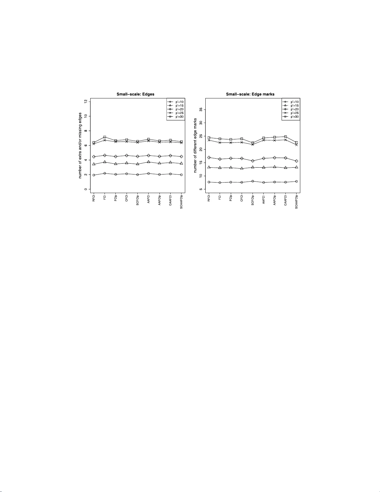
The Annals of Statistics 2012, V ol. 40, No. 1, 294–321 DOI: 10.1214 /11-AOS940 c  Institute of Mathematical Statistics , 2 012 LEARNING HIGH-DIMENSIONAL DIRECTED ACYCLIC GRAPHS WITH LA TENT AND SELECTION V ARIABLES By Diego Colombo 1 , Marlo e s H. Maa thuis 1 , Markus Kalisch and Thomas S. Richards on 2 ETH Z¨ urich, ETH Z ¨ urich, E TH Z¨ urich and University of W ashington W e consider the problem of learning causal information betw een random v ariables in directed acyclic graphs (DAGs) when allow ing arbitrarily many latent and selection v ariables. The FCI (F ast Causal Inference) algorithm has b een explicitly designed to infer conditional indep endence and causal information in su ch settings. H ow ever, FC I is computationally infeasible for large gra phs. W e therefore propose the new RFCI algorithm, which is m uch faster than FCI. In some situations the output of RFC I is slightly less informative, in particular with resp ect to conditional indep endence information. How ev er, we prov e that any causal information in th e outp ut of RFCI is correct in the asymptotic limit. W e also deﬁne a class of gra phs on which th e outputs of FC I and R FC I are identical. W e prov e consistency of FCI and RFCI in sparse h igh-dimensional settings, and demonstrate in sim ulations that the estimation p erformances of th e algorithms are very similar. All softw are is implemented in t h e R-pack age pcalg . 1. In tro duction. W e consider the pr oblem of learning the causal struc- ture b et we en r andom v ariables in acyc lic s y s tems with arbitrarily man y laten t an d selection v ariables. As backg roun d information, we ﬁrst discus s the situation w ithout laten t and selection v ariables in Section 1.1 . Next, in Section 1.2 w e discuss complications that arise w hen allo wing for arbitrarily man y latent and s election v ariables. Our n ew con tributions are outlined in Section 1.3 . Received Ap ril 2011; revised August 2011 . 1 Supp orted in part b y Swiss NSF Gran t 200021-129972 . 2 Supp orted in part b y U.S. NSF Grant CRI 0855230 and U.S. NIH Grant R01 AI032475. AMS 2000 subje ct classiﬁc ations. Primary 62H12, 62M45, 62-04; secondary 68T30. Key wor ds and phr ases. Causal structure learning, FC I algorithm, RFCI algorithm, maximal ancestra l graphs (MAGs), partial ancestral graphs (P AGs), high-dimensionality, sparsit y , consi stency . This is an electr onic r eprint of the original article published by the Institute o f Ma thematical Statistics in The Annals of Statistics , 2012, V ol. 40, No. 1, 2 94–32 1 . T his reprint diﬀers from the o riginal in pagination and typog raphic detail. 1 2 COLOMBO, MAA THUIS , KALISCH AND R ICHARDS O N 1.1. Systems without latent and sele ction var iables. W e ﬁr st consider sys- tems that satisfy the assump tion of causal suﬃciency , that is, that there are no un measured common causes and no un measured selection v ariables. W e assume that causal information b etw ee n v ariables can b e r epresen ted by a directed acyclic graph (D A G) in w h ic h the v ertices repr esen t random v ari- ables and th e edges represent direct causal eﬀects (see , e.g., [ 13 , 14 , 20 ]). In particular, X 1 is a direct cause of X 2 only if X 1 → X 2 (i.e., X 1 is a parent of X 2 ), and X 1 is a (p ossibly indirect) cause of X 2 only if there is a directed path from X 1 to X 2 (i.e., X 1 is an ancestor of X 2 ). Eac h causal D A G implies a set of conditional indep end ence relationships whic h can b e r ead oﬀ from the D A G using a concept called d -separation [ 13 ]. Sev eral D A Gs can describ e exactly the same co nditional indep endence infor- mation. Such D A Gs are called Mark o v equiv alent and form a Mark o v equiv- alence class. F or example, consider DA Gs on the v ariables { X 1 , X 2 , X 3 } . Then X 1 → X 2 → X 3 , X 1 ← X 2 ← X 3 and X 1 ← X 2 → X 3 form a Mark o v equiv al ence class, since they all imp ly the single conditional in d ep endence relationship X 1 ⊥ ⊥ X 3 | X 2 , that is, X 1 is conditionally indep end en t of X 3 giv en X 2 (using the shorthand notation of Da wid [ 7 ]). Another Mark o v equiv al ence class is giv en by the single D A G X 1 → X 2 ← X 3 , sin ce this is the only DA G that im p lies the conditional ind ep endence relationship X 1 ⊥ ⊥ X 3 alone. Mark o v equiv alence classes of D AG s can b e describ ed uniquely b y a completed p artially directed acyclic graph (CPDA G) [ 3 , 4 ]. CPD A Gs can b e learned from conditional indep end ence inform ation if one assumes faithfulness, that is, if the conditional indep endence relationships among the v ariables are exactly equal to those that are implied b y the DA G via d -separation. F or example, supp ose that the d istribution of { X 1 , X 2 , X 3 } is faithful to an unkno wn u nderlying causal D A G, and that th e only con- ditional ind ep endence relationship is X 1 ⊥ ⊥ X 3 | X 2 . Then the corresp ond ing Mark o v equiv alence class consists of X 1 → X 2 → X 3 , X 1 ← X 2 ← X 3 and X 1 ← X 2 → X 3 , and w e kn o w th at one of these three D A Gs m ust b e the true causal D A G. Algorithms that are based on this idea are calle d constrain t- based algorithms, and a prominent example is the PC algorithm [ 20 ]. The PC algorithm is sound (i.e., correct) and complete (i.e., maximally informa- tiv e) un der the assumptions of causal suﬃciency and faithfulness [ 20 ]. It is eﬃcien tly implemen ted in the R-pack age pcalg [ 9 ], and w as sh o wn to b e asymptotically consistent in spars e h igh-dimensional settings [ 8 ]. In practice, on e often w an ts to estimate n ot only the Mark o v equiv ale nce class of DA Gs, but also the size of causal eﬀects b et w een p airs of v ariables. In the sp ecial case th at the estimated CPD AG represen ts a single DA G, one can do this via, for example, P earl’s do-calc ulu s (also called in terv en tion cal- culus; see [ 13 ]) or marginal structural mo dels [ 18 ]. If the estimated CPD A G represent s sev eral D AG s, one can conceptually estimate causal eﬀects for eac h D A G in the Marko v equiv alence class, and u se these v alues to infer LEARNING DA GS WITH LA TENT AND SELECT ION V ARIABLES 3 b ound s on causal eﬀects. Th is idea, together with a fast lo cal implemen ta- tion, f orms th e b asis of the IDA algorithm [ 10 , 11 ] wh ich estimates b ound s on causal eﬀects from observ ational data th at are generated f rom an u nkno wn causal D A G (IDA stands for In terv enti on calculus when the D A G is Absent). The IDA algorithm was shown to b e consisten t in sparse h igh-dimensional settings [ 11 ], and w as v alidated on a c hallenging high-dimens ional y east gene expression data set [ 10 ]. 1.2. Complic ations arising f r om latent and sele ction variables. In prac- tice there are often laten t v ariables, that is, v ariables that are not mea- sured or recorded. Statistically sp eaking, these v ariables are marginalized out. Moreov er, there can b e selection v ariables, that is, unmeasured v ari- ables that determine whether or not a measured unit is included in the data sample. Statistically sp eaking, these v ariables are conditioned on (see [ 6 , 21 ] for a more detailed discussion). Laten t and selection v ariables cause sev eral complicatio ns. The ﬁrs t pr oblem is that causal inference based on the PC algorithm ma y b e incorrect. F or example, consider the D A G in Figure 1 (a ) with ob- serv ed v ariables X = { X 1 , X 2 , X 3 } and latent v ariables L = { L 1 , L 2 } . T h e only conditional in d ep endence relationship among th e observed v ariables is X 1 ⊥ ⊥ X 3 . Ther e is only one DA G on X th at implies th is single conditional indep end ence relationship, namely X 1 → X 2 ← X 3 , and this will ther efore b e th e outpu t of the PC algo rithm; see Fig ur e 1 (b). This output w ould lead us to b eliev e that b oth X 1 and X 3 are causes of X 2 . But this is clearly in - correct, since in the u nderlying D AG with laten t v ariables, there is neither a directed path from X 1 to X 2 nor one f rom X 3 to X 2 . A second problem is that the space of D A Gs is not closed un der marginal- ization and conditioning [ 16 ] in the follo wing sense. If a distribution is faith- ful to a D AG , then the distribution obtained by marginaliz ing out and co n- ditioning on some of the v ariables may not b e faithful to an y D A G on the observ ed v ariables. F or example, consider the D A G X 1 → X 2 ← L 1 → X 3 ← X 4 . This D A G implies the follo wing set of conditional ind ep endence relation- ships among the observed v ariables X = { X 1 , . . . , X 4 } : X 1 ⊥ ⊥ X 3 , X 1 ⊥ ⊥ X 4 , (a) (b) (c) Fig. 1. Gr aphs c orr esp onding to the examples in Se ction 1.2 . Thr oughout we use squar e b oxes to r epr esent latent variables and cir cles to r epr esent observe d variables. (a) DAG with late nt variables; ( b) CPDA G; (c) P A G. 4 COLOMBO, MAA THUIS , KALISCH AND R ICHARDS O N X 2 ⊥ ⊥ X 4 , X 1 ⊥ ⊥ X 3 | X 4 , X 1 ⊥ ⊥ X 4 | X 2 , X 1 ⊥ ⊥ X 4 | X 3 and X 2 ⊥ ⊥ X 4 | X 1 , and others implied by these. There is n o DA G on X that enta ils exactly this set of conditional indep endencies via d -separation. These problems can b e solv ed by in tro ducing a new class of graphs on the observed v ariables, called maximal ancestral graphs (MA Gs) [ 16 ]. Eve ry D A G with latent and selection v ariables can b e trans f ormed in to a unique MA G o v er the obser ved v ariables ([ 16 ], page 981 ). Sev eral DA Gs can lead to the same MA G. I n fact, a MA G describ es inﬁ nitely many D AG s sin ce no restrictions are m ade on the num b er of laten t and selection v ariables. MA Gs enco de ca usal rela tionships betw een the observed v ariables via th e edge marks. F or example, consider th e edge X 1 → X 2 in a MA G. The tail at X 1 implies that X 1 is a cause (ancestor) of X 2 or of a selection v ariable, and th e arrowhead at X 2 implies that X 2 is not a cause (not an ancestor) of X 1 nor of any s electio n v ariable, in all p ossible underlyin g D A Gs with laten t and selection v ariables. Moreo v er, MA Gs enco de conditional inde- p enden ce relationships among the observ ed v ariables via m -separation [ 16 ], a generalizatio n of d -separation (see Deﬁnition 2.1 in Section 2.2 ). Sev eral MA Gs can describ e exactly th e same conditional indep end ence r elation- ships; see [ 2 ]. Such MA Gs form a Mark o v equ iv alence class which can b e represent ed b y a partial ancestral graph (P AG); see Deﬁn ition 3.1 . P A Gs describ e causal features common to ev ery MAG in the Mark o v equiv alence class, and hence to ev ery D A G (possibly w ith laten t and selec tion v ariables) compatible with the observ able ind ep endence structure u nder the assump - tion of f aithfu lness. F or example, consider again the D A G in Figure 1 (a). The only conditional in d ep endence relationship among th e observed v ariables is X 1 ⊥ ⊥ X 3 , and this is represente d by the P AG in Figure 1 (c). This P A G implies that X 2 is not a cause (ancestor) of X 1 , X 3 or a s electio n v ariable, and this is indeed the case in the underlying D A G in Figure 1 (a) and is true of an y DA G that, assumin g faithfulness, could ha v e implied X 1 ⊥ ⊥ X 3 . The t w o circle mark s at X 1 and X 3 in Figure 1 (c) r epresen t uncertain t y ab out whether or not X 1 and X 3 are causes of X 2 . This reﬂects the fact that the single conditional ind ep endence relationship X 1 ⊥ ⊥ X 3 among the observ ed v ariables can arise from the D A G X 1 → X 2 ← X 3 in whic h X 1 and X 3 are causes of X 2 , but it can also arise fr om the DA G in Fig ure 1 (a) in whic h X 1 and X 3 are not causes of X 2 . Under the faithfulness assumption, a Marko v equiv alence class of D A Gs with laten t and selection v ariables can b e learned from cond itional indep en- dence information amo ng the observ ed v ariables alone using the F ast Causal Inference (F CI) algo rithm [ 20 ], which is a mo diﬁcation of the PC algorithm. Originally , the output of F CI w as deﬁned as a partially orien ted inducing path graph (POIPG), but its output can also b e inte rpr eted as a P A G [ 23 ]. Spirtes et al. [ 20 ] pro ve d that the F CI algo rithm is sound in the p resence of arbitrarily many la tent v ariables. Spirtes et al. [ 21 ] extended th e soundness LEARNING DA GS WITH LA TENT AND SELECT ION V ARIABLES 5 pro of to allo w for selec tion v ariables as w ell. Zhang [ 24 ] recen tly in tro du ced extra orien tation rules th at make FCI complete when its outpu t is int er- preted as a P AG. Despite its n ame, F CI is computationally very in tensive for large graph s. Spirtes [ 19 ] introdu ced a mo d iﬁed v ersion of F CI, called Anytime F CI, that only considers conditional indep endence tests with conditioning sets of size less than some presp eciﬁed cut-oﬀ K . Anytime F CI is t ypically faster but less in f ormativ e th an F CI, bu t the causal inte rpr etation of tails and arro wheads in its output is still s ou n d. Some w ork on the estimation of the size of causal eﬀects in situations with laten t and selection v ariables can b e foun d in [ 17 , 23 ] and in Chapter 7 of [ 20 ]. 1.3. New c ontributions. W e intro d uce a n ew algo rithm f or learning P A Gs, called the R e al ly F ast Caus al In ference (RF CI) algorithm (see S ection 3.2 ). RF CI u ses few er conditional ind ep endence tests than F CI, and its tests co n- dition on a smaller n umber of v ariables. As a result, RFCI is m uc h faster than FCI and its outp u t tends to b e more reliable for sm all samples, since conditional ind ep endence tests of high order hav e lo w p o w er. On the other hand, the output of RF CI m a y b e less informativ e. In this s ense, the algo- rithm is related to the Anytime F CI algorithm [ 19 ]. In Section 3.4 w e compare the outputs of F CI and RF CI, and deﬁne a class of graphs for which the outputs of FCI and RF CI are iden tical. In Section 4 we pro ve consistency of F CI and RF CI in sp arse high- dimensional settings. The sparsit y conditions needed for consistency of FCI are stronger than those for RFCI, du e to the h igher complexit y of the FCI algorithm. In order to compare RF CI to existing algorithms, we prop ose seve ral small mo diﬁ cations of F CI and An ytime FCI. In particular, w e in tro duce the Adaptiv e Anyti me FCI (AAF CI) algorithm (see Section 3 of the sup- plemen tary docu men t [ 5 ]) and w e p rop ose sev eral w a ys to sp eed up the F CI and AAF CI algorithms (see Section 3.1 ). W e sho w in sim ulations (see Section 5 ) that the n umb ers of errors made b y all algo rithms are ve ry similar. Moreo v er, we show that our mo diﬁcations of FCI and AAF CI sh orten the computation time considerably , but th at for large graphs , RF CI is the only f easible algorithm. All p ro ofs, a d escrip tion of AAF CI, pseud o co des and t w o additional exam- ples are giv en in the su pplemen tary do cument [ 5 ]. The R-pac k age pca lg [ 9 ] con tains implemen tations of all algorithms. 2. Preliminaries. This section introduces term in ology that is used thr ough- out the pap er. Section 2.1 deﬁnes v arious graphical concepts, and Secti on 2.2 describ es h ow graphs can b e in terpreted pr obabilistically and causally . 6 COLOMBO, MAA THUIS , KALISCH AND R ICHARDS O N 2.1. Gr aphic al deﬁnitions. A graph G = ( V , E ) is composed of a set of v ertices V = { X 1 , . . . , X p } and a set of edges E . In our framework, the ve r- tices represen t random v ariables and the edges d escrib e cond itional inde- p enden ce and ancestral relatio nsh ips. The edge set E can con tain (a s u b- set of ) the follo wing six t yp es of edges: → ( dir e cte d ), ↔ ( bi- dir e cte d ), − ( undir e cte d ), ❜ ❜ ( nondir e cte d ), ❜ ( p artial ly undir e cte d ) and ❜ → ( p artial ly dir e cte d ). Th e endp oin ts of an edge are called marks and they can b e tails , arr owhe ads or cir cles . W e use the symb ol “ ∗ ” to denote an arbitrary edge mark. A graph cont aining only directed edges is called dir e cte d , and one con taining only undirected edges is called undir e cte d . A mixe d graph can con tain directed, bi-directed and un directed edge s. If w e are only inte rested in the presence and absence of edges in a graph and not in the edge marks, w e r efer to the sk e leton of the graph. All the graphs we consider are si mple in that there is at most one edge b et we en an y t w o ve rtices. If an edge is present, the vertic es are said to b e adjac ent . If all pairs of v ertices in a graph are adjacent, the graph is called c om plete . The adjac ency set of a ve rtex X i in a graph G is th e set of all v ertices in V \ { X i } that are adjacen t to X i in G , d enoted b y adj( G , X i ). A ve rtex X j in adj( G , X i ) is called a p ar ent of X i if X j → X i , a child of X i if X i → X j , a sp ouse of X i if X i ↔ X j , and a neighb or of X i if X i − X j . The corresp ondin g sets of parents, children, sp ouses and neigh b ors are denoted b y pa( G , X i ), c h ( G , X i ), sp ( G , X i ) and n e( G , X i ), r esp ectiv ely . A p ath is a sequence of d istinct adjacen t v ertices. A p ath h X i , X j , . . . , X k i is said to b e out of ( into ) X i if the edge b et w een X i and X j has a tail (arro whead) at X i . A dir e c te d p ath is a path along directed edges that follo ws the direction of the arrowheads. A cycle o ccurs when there is a path from X i to X j and X i and X j are adjacent . A directed path from X i to X j forms a dir e cte d cycle together with the edge X j → X i , and it forms an almost dir e cte d cycle together with the edge X j ↔ X i . If there is a directed path π from X i to X j or if X i = X j , the v ertex X i is called an anc estor of X j and X j a desc endant of X i . The sets of ancesto rs and descendan ts of a v ertex X i in G are den oted by an ( G , X i ) and de( G , X i ), resp ectiv ely . T h ese deﬁnitions are applied to a set Y ⊆ V of distinct v ertices as follo ws: an( G , Y ) = { X i | X i ∈ an( G , X j ) for some X j ∈ Y } ; de( G , Y ) = { X i | X i ∈ de( G , X j ) for some X j ∈ Y } . Three vertic es that form a cycle are called a triangle . Th ree v ertices h X i , X j , X k i are called an unshielde d triple if X i and X j are adjacent , X j and X k are adj acen t, but X i and X k are n ot adjacen t. A non en dp oint v er- tex X j on a p ath π is a c ol lider on th e path if b oth the edges preceding and succeeding it ha v e an arro whead at X j , that is, if the path contai ns ∗ → X j ← ∗ . A nonendp oin t v ertex X j on a path π which is not a col lider is a non c ol lider on the path. An unsh ielded triple h X i , X j , X k i is called a v-structur e if X j is a collider on the path h X i , X j , X k i . LEARNING DA GS WITH LA TENT AND SELECT ION V ARIABLES 7 A path π = h X l , . . . , X j , X b , X p i in a mixed graph is called a discriminating p ath for X b if the follo wing three conditions hold: (i) π in cludes at lea st three edges; (ii) X b is a n onendp oin t v ertex on π and is adjacen t to X p on π ; and (iii) X l is not adjacen t to X p in the graph and ev ery ve rtex b et w een X l and X b is a collider on π and a paren t of X p . An example of a discrimin ating path is giv en in Figure 4 of [ 5 ], wh ere the circle m arks are r eplaced by stars. A graph G = ( V , E ) is called c onne cte d if there exists a path b et w een an y pair of v ertices in V . A graph is calle d bic onne cte d if it is connected and remains so if an y v ertex and its incident edges we re to b e remo v ed. A bic on- ne c te d c omp onent of a graph is a maximally biconnected su bgraph [ 1 ]. A directed graph G = ( V , E ) is called a dir e cte d acyclic gr aph (DA G) if it do es n ot con tain directed cycles. A mixed graph G = ( V , E ) is called an anc estr al gr aph if (i) it d o es not cont ain directed cycles, (ii) it do es not con tain almost d irected cycles, and (iii) for an y undirected edge X i − X j in E , X i and X j ha v e no parents or sp ouses. D A Gs form a subset of ancestral graphs. 2.2. Pr ob abilistic and c ausal interpr etation of g r aphs. A D A G ent ails conditional ind ep endence relationships via a graph ical criterion called d - separation, wh ic h is a sp ecial case of m -separation: Definition 2.1 (Ric hardson and Spirtes [ 16 ]). A path π in an ancestral graph is said to b e blo c k ed by a set of v ertices Y if and only if: (i) π con tains a subpath h X i , X j , X k i suc h that the mid dle vertex X j is a noncollider on this p ath and X j ∈ Y , or (ii) π con tains a v-stru cture X i ∗ → X j ← ∗ X k suc h that X j / ∈ Y and no descendan t of X j is in Y . V ertices Z and W are m -separated b y Y if ev ery path π b et w een Z and W is bloc ked by Y . S ets of v ertices Z and W are m -separated by Y if all pairs of ve rtices Z ∈ Z , W ∈ W are m -separated b y Y . If t w o v ertices X i and X j in a DA G G are d -separated by a subset Y of the remaining v ertices, then X i ⊥ ⊥ X j | Y in any distribution Q that factorizes according to G (i.e., the joint density can b e wr itten as the p ro duct of the conditional densities of eac h v ariable giv en its paren ts in G : q ( X 1 , . . . , X p ) = Q p i =1 q ( X i | pa( G , X i )). A d istr ibution Q is said to b e faithful to a DA G G if the r everse implication also holds, th at is, if the conditional indep endence relationships in Q are exa ctly the same as those that can b e inferred fr om G using d -separation. A set Y that d -separates X i and X j in a D A G is called a minimal sep ar ating set if no subs et of Y d -separates X i and X j . A set Y is a minimal sep ar ating set for X i and X j given S if X i and X j are d -separated b y Y ∪ S and there is n o subset Y ′ of Y su c h that X i and X j are d -separated b y Y ′ ∪ S . 8 COLOMBO, MAA THUIS , KALISCH AND R ICHARDS O N When a D A G G = ( V , E ) con tains latent and selectio n v ariables, we write V = X ˙ ∪ L ˙ ∪ S , where X represent s the observ ed v ariables, L represen ts the laten t v ariables and S represents the selection v ariables, and th ese sets are disjoin t (i.e., ˙ ∪ d enotes the union of disjoin t sets). A maximal anc estr al gr aph (MA G) is an ancestral graph in wh ic h ev- ery miss ing edge corresp onds to a cond itional indep en d ence relatio nsh ip. Ric hardson and S pirtes ([ 16 ], page 981) giv e an algorithm to transform a D A G G = ( X ˙ ∪ L ˙ ∪ S , E ) in to a u nique MA G G ∗ as follo w s. Let G ∗ ha v e v ertex set X . F or any pair of v ertices X i , X j ∈ X mak e them adjacen t in G ∗ if and only if th ere is an inducing p ath (see Deﬁn ition 3.5 ) b et w een X i and X j in G r elativ e to X giv en S . Moreo ve r, f or eac h edge X i ∗ ∗ X j in G ∗ put an arro whead at X i if X i / ∈ an( G , { X j } ∪ S ) and put a tail otherwise. The resu lting MAG G ∗ = ( X , E ∗ ) enco d es the conditional indep endence rela- tionships holding in G among the observ ed v ariables X conditional on some v alue for the select ion v ariables S = s ; thus if X i and X j are m -separated b y Y in G ∗ , then X i and X j are d -separated by Y ∪ S in G and hen ce X i ⊥ ⊥ X j | ( Y ∪ { S = s } ) in an y d istribution Q factorizing according to G . P erhaps more imp ortan tly , an ancestral graph p r eserv es the ancestral r ela- tionships enco ded in the D A G. Throughout th e remainder of th is pap er, S refers to either the set of v ariables S or the ev en t S = s , dep end in g on the con text. 3. Oracle v ersions of the algorithms. W e consider the follo wing problem: assuming that the distribution of V = X ˙ ∪ L ˙ ∪ S is faithfu l to an unkno wn underlying causal D A G G = ( V , E ) , and giv en oracle information ab out all conditional indep endence r elationships b et w een pairs of v ariables X i and X j in X giv en sets Y ∪ S where Y ⊆ X \ { X i , X j } , we w an t to infer in formation ab out the ancestral (causal) relationships of the v ariables in the underlying D A G, which w e represent via a P A G. W e discuss and compare t wo algorithms for this pur p ose, the F CI algo- rithm and our n ew RF CI algorithm. W e ﬁrst d eﬁne the outpu ts of b oth algorithms: an F CI-P A G and an RFCI-P A G. (An F CI-P A G is usually re- ferred to simply as a “P A G,” bu t in the remainder of this pap er w e u se the name F CI-P AG to make a clear distinction b et wee n the output of the tw o algorithms.) Definition 3.1. Let G b e a D A G with partitioned v ertex set X ˙ ∪ L ˙ ∪ S . Let C b e a simple graph with v ertex set X and edges of th e type → , ❜ → , ❜ ❜ , ↔ , − or ❜ . T hen C is said to b e an F CI-P A G that represen ts G if an d only if, f or any d istribution P of X ˙ ∪ L ˙ ∪ S that is faithful to G , the follo wing four conditions hold: (i) the absence of an edge b et w een tw o v ertices X i and X j in C implies that there exists a su bset Y ⊆ X \ { X i , X j } suc h that X i ⊥ ⊥ X j | ( Y ∪ S ) in P ; LEARNING DA GS WITH LA TENT AND SELECT ION V ARIABLES 9 (ii) the presence of an edge b et w een tw o v ertice s X i and X j in C implies that X i 6 ⊥ ⊥ X j | ( Y ∪ S ) in P for all subs ets Y ⊆ X \ { X i , X j } ; (iii) if an edge b et w een X i and X j in C has an arro whead at X j , then X j / ∈ an( G , X i ∪ S ) ; (iv) if an edge b et wee n X i and X j in C has a tail at X j , then X j ∈ an( G , X i ∪ S ). Definition 3.2. Let G b e a D A G with partitioned v ertex set X ˙ ∪ L ˙ ∪ S . Let C b e a simple graph with verte x set X a nd edges of the t yp e → , ❜ → , ❜ ❜ , ↔ , − , or ❜ . Then C is said to b e an RFCI-P A G that r epresen ts G if and only if, for an y distribu tion P of X ˙ ∪ L ˙ ∪ S that is faithful to G , conditions (i), (iii) and (iv) of Deﬁn ition 3.1 and the follo wing condition hold: (ii ′ ) the pr esence of an edge b etw een t wo ve rtices X i and X j in C implies that X i 6 ⊥ ⊥ X j | ( Y ∪ S ) for all subsets Y ⊆ adj( C , X i ) \ { X j } and for all su b sets Y ⊆ adj( C , X j ) \ { X i } . Condition (ii) in Deﬁnition 3.1 is s tr onger than condition (ii ′ ) in Deﬁ- nition 3.2 . Hence, th e presence of an edge in an RF CI-P AG has a weak er in terpretation than in an F CI-P A G. This has sev eral co nsequ ences. First, ev- ery F CI-P A G is an RFCI-P A G. S econd, diﬀeren t RF CI-P A Gs for the same underlying D A G ma y hav e diﬀeren t ske letons, while the F CI-P A G skel eton is unique. In general, the RF CI-P A G s kelet on is a su p ergraph of the FCI-P A G sk eleton. Finally , an RF CI-P A G can corresp ond to more th an one Marko v equiv al ence class of D A Gs (see Example 2 in S ection 3.3 ). It is w orth noting that ev ery FCI-P A G is an RF CI-P A G. Moreo v er, for a giv en pair of a graph G and a distribution P f aithful to it, there may b e t wo diﬀeren t FCI-P A Gs that represen t G b ut they will hav e the s ame sk eleton. On the other hand, for a giv en pair of a graph G and a distr ib ution P faithful to it, ther e ma y also b e more th an one RFCI-P A G that represent s G and these diﬀerent RF CI-P AGs can also ha v e diﬀerent sk eleto ns. The r emainder of this section is organized as follo ws. S ection 3.1 brieﬂy discusses the F CI algorithm and p rop oses mo diﬁ cations that can sp eed up the algorithm while r emaining sound and complete. S ection 3.2 in tro duces our new RF CI algorithm. Section 3.3 discu s ses sev eral examples that illus- trate the commonalities and diﬀerences b et w een the t wo algorithms, and Section 3.4 d eﬁnes a cla ss of graph s for whic h the outputs of F CI and RFCI are identic al. 3.1. The FCI algorithm. A high-lev el sketc h of F CI ([ 20 ], pages 144 and 145) is giv en in Algorithm 3.1 . The sub-algorithms 4.1– 4.3 are giv en in [ 5 ]. The determination of adjacencies in the P AG within the F CI alg orithm is based on th e follo wing fact: if X i is not an ancestor of X j , and X i and X j are conditionally indep enden t giv en some set Y ∪ S where Y ⊆ X \ { X i , X j } , 10 COLOMBO, MAA THUIS , KALISCH AND R ICHARDS O N Algorithm 3.1 The F CI algorithm Require: Conditional independence information among all v ariables in X given S 1: Use Algorithm 4.1 of [ 5 ] to ﬁ nd an initial skeleton ( C ), separation sets (sepset) and unshielded triple list ( M ); 2: Use Algorithm 4.2 of [ 5 ] to orien t v-struct u res (upd ate C ); 3: Use Algorithm 4.3 of [ 5 ] to ﬁnd the ﬁnal ske leton (up d ate C and sepset); 4: Use Algorithm 4.2 of [ 5 ] to orien t v-struct u res (upd ate C ); 5: Use rules (R1)–(R10) of [ 24 ] to orien t as many edge marks as p ossible ( up date C ); 6: return C , sepset. then X i and X j are conditionally indep endent giv en Y ′ ∪ S for some sub- set Y ′ of a certain set D-SEP( X i , X j ) or of D-SEP ( X j , X i ) (see [ 20 ], p age 134 for a deﬁnition). This means th at, in ord er to determine w hether there is an edge b et w een X i and X j in an F CI-P AG, one do es not need to test whether X i ⊥ ⊥ X j | ( Y ∪ S ) for all p ossible sub sets Y ⊆ X \ { X i , X j } , b ut only for all p ossible su bsets Y ⊆ D-SEP( X i , X j ) and Y ⊆ D-SEP( X j , X i ). Sin ce the s ets D-SEP( X i , X j ) cannot b e inferred from the observed conditional indep en- dencies, Sp irtes et al. [ 20 ] deﬁned a sup erset, calle d Po ssible-D-SEP , that can b e computed: Definition 3.3. Let C b e a graph with an y of the follo wing edge t yp es: ❜ ❜ , ❜ → , ↔ . P ossible-D-SEP ( X i , X j ) in C , denoted in s h orthand b y p ds( C , X i , X j ), is deﬁned as follo ws: X k ∈ p d s( C , X i , X j ) if and only if there is a path π b et w een X i and X k in C such that for ev ery s u bpath h X m , X l , X h i of π , X l is a collider on the su bpath in C or h X m , X l , X h i is a triangle in C . Remark 3.1. Note that X j do es not p lay a role in the deﬁnition of p ds( C , X i , X j ), but we keep it as an argumen t b ecause we will late r con- sider alt ernative deﬁnitions of P ossible-D-SEP (see Deﬁnition 3.4 ) wh ere the second vertex X j do es pla y a role. Since the deﬁnition of Possible-D-SEP requ ires some kn o wledge ab out the skel eton and orien tation of ed ges, the F CI algorithm ﬁrst ﬁnds an initial sk eleton denoted by C 1 in Step 1. This is done as in the PC-algorithm, b y starting with a complete graph with edges ❜ ❜ and p erform ing cond itional indep end ence tests giv en subs ets of increasing size of the adj acency sets of the v ertices. An edge b et w een X i and X j is deleted if a conditional indep en- dence is foun d, and the set resp ons ib le for this conditional indep endence is sa v ed in sepset( X i , X j ) and sepset( X j , X i ) (see Algorithm 4.1 of [ 5 ]). The sk eleton after completion of Step 1 is a sup erset of the ﬁn al sk eleton. In Step 2, the algorithm orients unsh ielded triples X i ∗ ❜ X j ❜ ∗ X k as v- structures X i ∗ → X j ← ∗ X k if and only if X j is n ot in sepset( X i , X k ) and sepset( X k , X i ) (see Algorithm 4.2 of [ 5 ]). The graph r esulting after Step 2, denoted by C 2 , cont ains suﬃcien t in - formation to compute the Po ssible-D-SEP sets. Th us, in Step 3, the algo - LEARNING DA GS WITH LA TENT AND SELECT ION V ARIABLES 11 rithm computes p ds( C 2 , X i , · ) for ev ery X i ∈ X . Then for ev ery elemen t X j in adj( C 2 , X i ), the algorithm tests whether X i ⊥ ⊥ X j | ( Y ∪ S ) for every su bset Y of p ds( C 2 , X i , · ) \ { X i , X j } and of p ds( C 2 , X j , · ) \ { X j , X i } (see Algorithm 4.3 of [ 5 ]). As in Step 1, the tests are arranged in a h ierarc hical w a y starting with conditioning sets of small size. If there exists a set Y that make s X i and X j conditionally indep end en t giv en Y ∪ S , th e edge b et w een X i and X j is remo v ed and the set Y is sa v ed as the separation set in s ep set( X i , X j ) and s ep set( X j , X i ). After all conditional indep endence tests are completed, ev ery edge in C is r eorien ted as ❜ ❜ , since the orienta tion of v-stru ctures in S tep 2 of the algorithm cannot necessarily b e interpreted as sp eciﬁed in conditions (iii) and (iv) of Deﬁnition 3.1 . In S tep 4, the v-structures are therefore orien ted again based on the u p- dated sk eleton and the up dated information in sepset (see Algorithm 4.2 of [ 5 ]). Finally , in Step 5 the algorithm replaces as m an y circles as p ossible b y arro wheads and tails using th e orien tation rules describ ed b y [ 24 ]. First pr op ose d mo diﬁc ation: FCI path . F or spars e graphs, Step 3 of the F CI algorithm dr amatical ly increases the compu tational complexit y of th e algorithm when compared to the PC algorithm. The additional computa- tional eﬀort can b e divided in t wo parts: co mpu ting the P ossible-D-SEP sets, and testing conditional in dep end en ce giv en all subsets of these sets. The lat- ter part is compu tationally infeasible when the sets p d s( C 2 , X i , · ) are large, con taining, sa y , more than 30 ve rtices. S ince the s ize of the P ossible-D-SEP sets plays suc h an imp ortan t role in the complexit y of the F CI algorithm, and since one has some freedom in deﬁnin g these sets (they simply must b e sup ers ets of the D-SEP sets), w e ﬁ rst prop ose a mo diﬁcation of the deﬁn ition of Po ssible-D-SEP that can decrease its s ize. Definition 3.4. Let C b e a graph with an y of the follo wing edge t yp es: ❜ ❜ , ❜ → , ↔ . T hen, for tw o v ertices X i and X j adjacen t in C , p ds path ( C , X i , X j ) is deﬁ ned as follo ws: X k ∈ p ds path ( C , X i , X j ) if and only if (i) there is a p ath π b et we en X i and X k in C suc h that for every su bpath h X m , X l , X h i of π , X l is a collider on the subpath in C or h X m , X l , X h i is a triangle in C , an d (ii) X k lies on a path b et w een X i and X j . F or any pair of adjacen t v ertices X i and X j in a graph C , the s et p d s path ( C , X i , X j ) can b e computed easily b y int ersecting p d s( C , X i , · ) with the unique biconnected comp onen t in C that con tains the edge b et w een X i and X j . Algorithm 4.3 of [ 5 ] can no w b e mo diﬁed as follo ws. Before lin e 1, we compute all biconnecte d comp onen ts of the graph C 2 , w here C 2 is the graph resulting from Step 2 of the FCI algo rithm. Then b et wee n lines 3 and 4, w e compute p ds path ( C 2 , X i , X j ) as d escrib ed ab o ve. Finally , on lines 8, 13 and 14, we replace p ds( C 2 , X i , · ) by p ds path ( C 2 , X i , X j ). W e refer to the F CI algorithm with this mo diﬁed ve rsion of Algorithm 4.3 of [ 5 ] as FCI path . 12 COLOMBO, MAA THUIS , KALISCH AND R ICHARDS O N Se c ond class of mo diﬁc ations: CF CI, CFCI path , SCF CI and SCFCI path . Another p ossibilit y to decrease the size of Possible-D -SEP is to u se conserv a- tiv e rules to orien t v-structures in Step 2 of the F CI algorithm, so that few er arro wheads are intro d uced, similarly to the Conserv ativ e PC algorithm [ 15 ]. This is esp ecially helpful in the sample version of the algorithm (see Sec- tion 4.1 ), as the sample v ersion tends to orient too many v-structures, whic h can lead to lo ng c hains of bi-dir ected edges and hence large Possible-D -SEP sets (see Figure 6 in S ection 5.3 ). The conserv ativ e orienta tion works as follo ws. F or all unsh ielded triples h X i , X j , X k i in C 1 , w here C 1 is the graph resulting from Step 1 of the FCI algorithm, w e determine all s ubsets Y of adj( C 1 , X i ) and of adj ( C 1 , X k ) sat- isfying X i ⊥ ⊥ X k | ( Y ∪ S ). W e refer to these sets as separating sets, and we lab el the triple h X i , X j , X k i as unambiguous if and only if (i) at least one separating set Y is found and either X j is in all separating s ets an d in sepset( X i , X k ) or X j is in none of the separating sets nor in sepset( X i , X k ), or (ii) no s uc h separating set Y is found. [Cond ition (ii) can o ccur, since sep- arating sets foun d in Step 1 of the F CI algorithm do not need to b e a su bset of adj( C 1 , X i ) or of adj( C 1 , X k ).] A t th e end of Step 2, w e only orien t un- am biguous triples satisfying X j / ∈ sepset( X i , X k ) as v-structures. This may lead to diﬀeren t P ossible-D-SEP sets in Step 3 (ev en in the oracle v ersion of the alg orithm), but other than that, Steps 3–5 of the algorithm remain unc hanged. W e refer to this version of the F CI alg orithm as Conserv ativ e F CI (CF CI). If CF CI is used in com bination with p ds path , w e use the name CF CI path . Finally , th e idea of conserv ativ e v-structures can also b e applied in S tep 4 of the FCI algorithm. F or eac h unsh ielded triple h X i , X j , X k i in C 3 , where C 3 is the graph resulting from S tep 3, we determine all subsets Y of ad j ( C 3 , X i ) and of adj( C 3 , X k ) satisfying X i ⊥ ⊥ X k | ( Y ∪ S ) . W e then determine if a triple is unambiguous, and only if this is th e case w e orien t it as v-structure or non-v-structure. Moreo v er, the orient ation rules in Step 5 of the algorithm are adapted so that they only rely on u nam biguous triples. W e use the name Sup erconserv ativ e F CI (SC F CI) to refer to the v ersion of F CI that uses con- serv ati ve v-structures in b oth Steps 2 and 4. If SCFCI is used in com bination with p d s path , w e use the name S CF CI path . The pro of of Theorem 3.1 sho ws that the output of the orac le version of SCF CI is iden tical to that of CF CI. W e still consider this version, ho we ve r, in the h op e to obtain b etter edge orien tations in the sample versions of the algorithms, where the outputs are t ypically not identi cal. Soundn ess of FCI follo ws from Theorem 5 of [ 21 ]. Sound ness resu lts f or the mo diﬁ cations FCI path , CF CI, CF CI path , SCFCI and S CF CI path are giv en in the f ollo wing theorem: Theorem 3.1. Consider one of the or acle versions of F CI path , CFCI, CF CI path , SCFCI or SCFCI path . L et the distribution of V = X ˙ ∪ L ˙ ∪ S b e LEARNING DA GS WITH LA TENT AND SELECT ION V ARIABLES 13 faithful to a DA G G and let c onditio nal i ndep endenc e information among al l v ariables in X giv e n S b e the input to the algorithm. Then the output of the algorithm i s an FCI-P AG of G . Completeness of FCI was pro ve d by [ 24 ]. This means th at the output of F CI is maximally informativ e, in the sense that for every circle mark there exists at least one MA G in the Mark o v equiv alence class represen ted b y the P AG w here the mark is oriented as a tail, and at least one where it is oriente d as an arro whead. Completeness results of F CI path , CF CI, CF CI path , SCF CI and SCF CI path follo w directly f r om the fact that, in the oracle v ersions, th e orien tation rules of these modiﬁ cations b oil down to the orien tation rules of F CI. 3.2. The RF CI algorithm . T h e Really F ast Cau s al Inference (RF CI) al- gorithm is a mo diﬁcation of F CI. The m ain diﬀerence is that RF CI a v oids the conditional indep end ence tests giv en su bsets of P ossible-D-SEP sets, whic h can b ecome very large ev en f or sparse graphs. I n stead, RF CI p er- forms some additional tests b efore orien ting v-structur es an d discriminating paths in order to ensu re soundness, based on Lemmas 3.1 and 3.2 b elo w. The num b er of these additional tests and the s ize of their cond itioning sets is sm all f or sp arse graphs, since RFCI only conditions on subsets of the adja- cency sets. As a resu lt, RF CI is m uch faster than F CI for sp arse graphs (see Section 5.3 ). Moreo ve r, the lo we r compu tational complexit y of RFCI leads to h igh-dimensional consistency r esults u nder weak er conditions than F CI [compare conditions (A3) and (A3 ′ ) in Sections 4.2 and 4.3 ]. A h igh-lev el sk etc h of RFCI is giv en in Algorithm 3.2 . Step 1 of the algorithm is identica l to S tep 1 of Algorithm 3.1 , and is used to ﬁnd an initial sk eleton C 1 that s atisﬁes conditions (i) and (ii ′ ) of Deﬁnition 3.2 . In Step 2 of the alg orithm, u nshielded triples are orien ted based on Lem- ma 3.1 and some further edges m ay b e remov ed. Lemma 3.1 (Unshielded triple ru le). L e t the distribution of V = X ˙ ∪ L ˙ ∪ S b e faithful to a DA G G . Assume tha t (a1) S ik is a minimal sep ar ating set Algorithm 3.2 The RF CI algorithm Require: Conditional independence information among all v ariables in X given S 1: Use Algorithm 4.1 of [ 5 ] to ﬁ nd an initial skeleton ( C ), separation sets (sepset) and unshielded triple list ( M ); 2: Use Algorithm 4.4 of [ 5 ] to orien t v-struct u res (upd ate C and sepset); 3: Use Algorithm 4.5 of [ 5 ] to orient as many edge marks as p ossible (upd ate C and sepset); 4: return C , sepset. 14 COLOMBO, MAA THUIS , KALISCH AND R ICHARDS O N for X i and X k given S , and (a2) X i and X j as wel l as X j and X k ar e c on- ditional ly dep endent given ( S ik \ { X j } ) ∪ S . Then X j ∈ an( G , { X i , X k } ∪ S ) if and only if X j ∈ S ik . The details of Step 2 are giv en in Algorithm 4.4 of [ 5 ]. W e start with a list M of all unshielded triples in C 1 , where C 1 is the graph resulting f rom Step 1 of the RF CI algorithm, and an empty list L th at is used to store triples that were found to satisfy the conditions of Lemma 3.1 . F or eac h triple h X i , X j , X k i in M , w e c hec k if b oth X i and X j and X j and X k are conditionally d ep endent giv en (sepset( X i , X k ) \ { X j } ) ∪ S . These conditional dep end en cies ma y not ha ve b een chec ked in Step 1 of the algorithm, s in ce sepset( X i , X k ) \ { X j } d o es n ot n eed to b e a sub set of adj( C 1 , X j ). If b oth con- ditional dep en d encies hold, the trip le satisﬁes the conditions of L emm a 3.1 and is added to L . On the other han d , an add itional conditional ind ep end- ence relationship ma y b e detected, sa y X i ⊥ ⊥ X j | ((sepset( X i , X k ) \ { X j } ) ∪ S ). This ma y arise in a situation wh ere X i and X j are n ot m -separated giv en a sub s et of v ertices adjacen t to X i , and are not m -separated giv en a subset of vertic es adjacent to X j , but th ey do happ en to b e m -separated giv en the set (sepset( X i , X k ) \ { X j } ) ∪ S . In this situation, we remo v e the edge X i ∗ ∗ X j from the graph, in agreemen t with condition (i) of Deﬁnition 3.2 . The remo v al of this edge can creat e new unshielded triples, which are added to M . Moreo v er, it can destroy u nshielded triples in L and M , whic h are therefore remov ed. Finally , by testing su b sets of the conditioning set whic h led to r emo v al of the edge, w e ﬁ nd a minimal separating set for X i and X j and store it in s ep set( X i , X j ) and sepset( X j , X i ). Example 1 of [ 5 ] shows that it is n ot suﬃcient to simply store sepset( X i , X k ) \ { X j } since it may not b e m inimal for X i and X j . W e wo rk with the lists M a nd L to en- sure that the result of Step 2 do es not dep end on the order in wh ic h the unshielded triples are considered. After Step 2, all unshielded tr iples still p resen t in the graph are co rrectly orien ted as a v-structure or n on-v-structure. In S tep 3, the algorithm orien ts as m any fu rther edges as p ossible, as describ ed in Algorithm 4.5 of [ 5 ]. This pro cedure consists of rep eated applications of th e orientati on rules (R1)– (R10) of [ 24 ], with th e diﬀerence that ru le (R4) ab out the discr im in ating path has b een mo diﬁed according to Lemma 3.2 . Lemma 3.2 (Discriminating path r ule). L et the distribution of V = X ˙ ∪ L ˙ ∪ S b e faithful to a DA G G . L et π ik = h X i , . . . , X l , X j , X k i b e a se qu e nc e of at le ast four vertic es that satisfy: (a1) X i and X k ar e c onditional ly inde- p endent given S ik ∪ S , (a2) any two suc c essive vertic es X h and X h +1 on π ik ar e c onditiona l ly dep endent given ( Y ′ \ { X h , X h +1 } ) ∪ S for al l Y ′ ⊆ S ik , (a3) al l vertic es X h b etwe en X i and X j (not including X i and X j ) satisfy X h ∈ an( G , X k ) and X h / ∈ an( G , { X h − 1 , X h +1 } ∪ S ) , wher e X h − 1 and X h +1 LEARNING DA GS WITH LA TENT AND SELECT ION V ARIABLES 15 denote the vertic es adjac ent to X h on π ik . Then the fol lowing hold: (b1) if X j ∈ S ik , then X j ∈ an( G , { X k } ∪ S ) and X k / ∈ an ( G , { X j } ∪ S ) , and (b2) if X j / ∈ S ik , then X j / ∈ an( G , { X l , X k } ∪ S ) and X k / ∈ an ( G , { X j } ∪ S ) . Lemma 3.2 is applied as f ollo ws. F or eac h triangle h X l , X j , X k i of the form X j ❜ ∗ X k , X j ∗ → X l and X l → X k , the algorithm searches for a discrim in ating path π = h X i , . . . , X l , X j , X k i for X j of minimal length, and c h ec ks that the v ertices in ev ery consecutiv e pair ( X r , X q ) on π are conditionally d ep endent giv en Y ∪ S for al l subsets Y of sepset( X i , X k ) \ { X r , X q } . (Example 2 of [ 5 ] sho ws wh y it is not suﬃ cien t to only c hec k conditional d ep endence giv en (sepset( X i , X k ) \ { X r , X q } ) ∪ S , as we did for the v-stru ctur es.) If we do not ﬁnd an y conditional ind ep endence relationship, the path satisﬁes the conditions of Lemma 3.2 and is orien ted as in rule (R4) of [ 24 ]. If one or more conditional in d ep endence relationships are found, the corresp ond ing edges are remo v ed, their minimal sep arating sets are stored, and any n ew unshielded tr ip les that are created by remo ving th e edges are orien ted u sing Algorithm 4.4 of [ 5 ]. W e note that the output of Step 3 ma y dep end on the order in wh ic h the discriminating p aths are considered. Soundn ess of RF CI is stated in the follo wing theorem. Theorem 3.2. L et the d istribution of V = X ˙ ∪ L ˙ ∪ S b e faithful to a DAG G and let c onditional indep endenc e information among al l v ariables in X give n S b e the i nput to the RF CI algorithm. Then the output of RFCI is an RFCI-P AG of G . Remark 3.2. Th e new orien tation rules b ased on Lemmas 3.1 and 3.2 op en p ossibilities for diﬀeren t modiﬁ cations of the F CI algo rithm. F or exa m- ple, one could replace p ds( C , X i , X j ) by p ds k ( C , X i , X j ), w h ere a vertex X l is in p d s k ( C , X i , X j ) if it is in p ds( C , X i , X j ) and there is a p ath betw een X i and X l con taining no m ore than k + 1 v ertices. This mo diﬁcation yields a skeleto n that is t ypically a s u p erset of the skelet on of the true FCI-P A G. In order to infer correct causal orien tatio ns b ased on this sk eleto n, one needs to use Algorithms 4.4 and 4.5 of [ 5 ] to d etermine the ﬁ nal orienta tions of the edges. The parameter k r epresen ts a trade-oﬀ b et wee n computing time and in formativ eness of the output, wh ere k = 1 corresp onds to the RFCI algorithm and k = | X | − 2 corresp on d s to the FCI algorithm. Another wa y to ob tain a more informativ e but slow er version of RF CI can b e obtained by mo difying Step 1 of th e RF CI algorithm: in s tead of considering all subsets of adj( C , X i ) and of adj( C , X j ), one can consider all subsets of the union adj ( C , X i ) ∪ adj( C , X j ). 3.3. Examples. W e now illustrate the algorithms in t w o examples. In Example 1 , the outputs of FCI and RF CI are identica l. In Example 2 , the outputs of FCI and RFCI are not ident ical, and the output of RF CI describ es t w o Mark o v equiv alence classes. W e will s ee, ho we ve r, that the ancestral or 16 COLOMBO, MAA THUIS , KALISCH AND R ICHARDS O N (a) (b) (c) Fig. 2. Gr aphs c orr esp onding to Example 1 , wher e the outputs of F CI and RFCI ar e identic al. (a) Underlying DA G with latent variables; (b) initial skeleton C 1 ; (c) RFCI-P AG and FCI-P AG. causal in formation inf er r ed from an RF CI-P AG is correct. Two additional examples illustrating details of Algorithms 4.4 and 4.5 of [ 5 ] are giv en in Section 5 of [ 5 ]. Example 1. Consider the D A G in Figure 2 (a) conta ining obser ved v ariables X = { X 1 , . . . , X 6 } , laten t v ariables L = { L 1 , L 2 } and n o selection v ariables ( S = ∅ ). Supp ose that all conditional indep endence r elationships o v er X that can b e read oﬀ from this D A G are used as input for the algo- rithms. In all algorithms, S tep 1 is the same, and consists of ﬁnd in g an initial sk eleton. This sk eleton, denoted b y C 1 , is s h o wn in Figure 2 (b). The ﬁ nal output giv en by b oth algorithms is sh o wn in Figure 2 (c). Comparing the initial sk eleton with the ﬁ nal skele ton, w e see th at the edge X 1 ❜ ❜ X 5 is pr esen t in the initial bu t not in the ﬁ n al ske leton. The absence in the ﬁ n al sk eleton is du e to the fact that X 1 ⊥ ⊥ X 5 |{ X 2 , X 3 , X 4 } . The edge is pr esen t in the initial skele ton, sin ce this conditional indep en dence is not found in Step 1 of the algorithms, b ecause { X 2 , X 3 , X 4 } is not a subset of adj( C 1 , X 1 ) n or of adj ( C 1 , X 5 ). The F CI algorithm ﬁn ds the co nditional indep end ence relati onship X 1 ⊥ ⊥ X 5 |{ X 2 , X 3 , X 4 } in Step 3 when s ubsets of P ossible-D-SEP are consid- ered, since p ds( C 2 , X 1 , X 5 ) \ { X 1 , X 5 } = { X 2 , X 3 , X 4 } and p ds( C 2 , X 5 , X 1 ) \ { X 5 , X 1 } = { X 2 , X 3 , X 4 , X 6 } , where C 2 is the graph resulting from Step 2 of the algorithm. In the RFCI algorithm, the conditional indep endence relatio nsh ip X 1 ⊥ ⊥ X 5 | { X 2 , X 3 , X 4 } is also foun d, b ut by another mec hanism. In Step 2 of Al- gorithm 3.2 , unshielded triples are oriented after p erforming some addi- tional conditional in dep enden ce tests. In particular, when considerin g the triple h X 1 , X 5 , X 6 i , the algorithm chec ks whether X 1 ⊥ ⊥ X 5 | (sepset( X 1 , X 6 ) \ { X 5 } ), wh ere sepset( X 1 , X 6 ) = { X 2 , X 3 , X 4 } . LEARNING DA GS WITH LA TENT AND SELECT ION V ARIABLES 17 (a) (b) (c) Fig. 3. Gr aphs c orr esp onding to Example 2 , wher e the outputs of F CI and RFCI ar e not identic al. The output of RFCI c orr esp onds to two Markov e quivalenc e classes when interpr ete d as an RF CI-P AG. (a) Underlying DA G G with latent variables; (b ) output of RFCI for G ; (c) output of F CI for G . This example also sho ws why it is necessary to chec k unsh ielded tr iples according to Lemma 3.1 b efore orient ing them as v-structures. Omitting this c hec k for triple h X 1 , X 5 , X 6 i wo uld o rient it as a v-structure, since X 5 / ∈ sepset( X 1 , X 6 ). Hence, w e wo uld conclude that X 5 / ∈ an ( G , { X 6 } ∪ S ), whic h con tradicts th e und erlying D A G. Finally , w e see that the orien tations of the edges are iden tical in the outputs of b oth algorithms, whic h implies that the outputs enco de the same ancestral inform ation. Example 2. Consider the D A G G in Figure 3 (a), conta ining observ ed v ariables X = { X 1 , . . . , X 5 } , laten t v ariables L = { L 1 , L 2 } and n o selection v ariables ( S = ∅ ) (see also [ 21 ], page 228, Figure 8a). Sup p ose th at all con- ditional indep end ence relationships ov er X that can b e read oﬀ fr om this D A G are used as input for the algorithms. The outputs of the RF CI and FCI algorithms are shown in Figure 3 (b) and (c), resp ectiv ely . W e see that the output of RFCI con tains an extra edge, namely X 1 ↔ X 5 . As in Example 1 , this edge is presen t after Step 1 of b oth algorithms. The reason is that th e conditional indep end ence X 1 ⊥ ⊥ X 5 |{ X 2 , X 3 , X 4 } is not found, because { X 2 , X 3 , X 4 } is not a subset of adj( C 1 , X 1 ) nor of adj( C 1 , X 5 ), where C 1 denotes the sk eleton after Step 1. The F CI algorithm ﬁnds this conditional indep endence in Step 3 when subsets of Possible-D-SEP are considered . Th e RFCI algorithm d o es n ot ﬁnd this conditional indep end ence, since the edge b et w een X 1 and X 5 do es not app ear in an un shielded triple or a discriminating p ath. Ho w ev er, the ancestral information enco d ed b y the output of RFCI is correct, and in this example ident ical to the ancestral information enco ded b y the output of F CI. Finally , w e sho w that the RF CI-P A G in Figure 3 (b) describ es t w o Mark o v equiv al ence classes. Consider a new D A G G ′ , which is adapted from G in Fig- 18 COLOMBO, MAA THUIS , KALISCH AND R ICHARDS O N ure 3 (a) by adding one add itional laten t v ariable L 3 p oint ing at X 1 and X 5 . This mod iﬁcation implies that X 1 and X 5 are conditional ly dep enden t giv en an y subs et of the r emaining observed v aria bles, so that G ′ b elongs to a dif- feren t Mark o v equiv alence cla ss than G . The output of b oth F CI and RFCI, when using as inp u t the conditional indep end ence relationships that can b e read oﬀ from G ′ , is giv en in Figure 3 (b). Hence, the P A G in Figure 3 (b) rep- resen ts more than one Marko v equiv alence class if interpreted as an RF CI- P AG. 3.4. A class of gr aphs for which the outputs of F CI and RFCI ar e identi- c al . W e no w sp ecify graphical conditions on an underlying DA G G = ( V , E ) with V = X ˙ ∪ L ˙ ∪ S suc h that the outputs of F CI and RF CI are ident ical (Theorem 3.3 ). Moreo ver, if the outputs of RF CI and FCI are not identical , w e inf er prop erties of edges that are present in the output of RF CI bu t not in that of F CI (Th eorem 3.4 ). The results in this s ection rely on th e concept of ind ucing paths [ 21 , 22 ], whic h we ha v e extended here: Definition 3.5. L et G = ( V , E ) b e a D A G with V = X ˙ ∪ L ˙ ∪ S and let Y b e a subset of X con taining X i and X j with X i 6 = X j . A path π b et we en X i and X j is called an inducing p ath r elative to Y given S if and only if ev ery mem b er of Y ∪ S that is a nonen dp oint on π is a collider on π and ev ery collider on π has a descendant in { X i , X j } ∪ S . W e note that our Deﬁnition 3.5 corresp onds to the one in [ 21 ] if Y = X . The existe nce of an in ducing path in a DA G is related to d -connection in the follo wing wa y . T h ere is an indu cing path b et w een X i and X j relativ e to Y giv en S if and only if X i and X j are not d -separated by ( Y ′ ∪ S ) \ { X i , X j } for all Y ′ ⊆ Y (see [ 21 ], Lemma 9, page 243). The d eﬁnition of an inducing path is monotone in th e follo wing sense: if Y 1 ⊆ Y 2 ⊆ X and th ere is an inducing path b et w een X i and X j relativ e to Y 2 giv en S , then there also is an ind ucing path b et wee n X i and X j relativ e to Y 1 giv en S . Consider a pair of v ertices X i , X j ∈ X in an underlyin g D A G G . W e in- tro duce the follo wing sh orthand notation. Let Adj ( i, j ) = adj( C 1 , X i ) \ { X j } , where C 1 is the initial sk eleton after Step 1 of the algorithms. Moreo v er, let Pds( i, j ) = p ds( C 2 , X i , X j ) \ { X j , X i } , where C 2 is the graph resulting from Step 2 of the F CI algorithm. By deﬁnition, Pd s ( k , i ) ⊇ Adj( k , i ) for an y pair of ve rtices X k , X i ∈ X . W e n o w consider the follo wing three scenarios: (S1) There is an inducing path b et w een X i and X j in G relat ive to Pds( i, j ) giv en S , and there is an in d ucing path b et w een X i and X j rel- ativ e to Pds ( j, i ) giv en S . (S2) There is an inducing path b et w een X i and X j in G relat ive to Adj( i, j ) giv en S , and th ere is an ind u cing path b et w een X i and X j relativ e to Adj( j, i ) given S . Moreo v er, there is n o inducing path b et w een X i and X j LEARNING DA GS WITH LA TENT AND SELECT ION V ARIABLES 19 in G relativ e to P d s( i, j ) giv en S , or there is n o in d ucing path b etw een X i and X j in G relativ e to Pds ( j, i ) give n S . (S3) There is no inducing path b et w een X i and X j in G relat ive to Adj( i, j ) given S , or there is n o inducing p ath b et w een X i and X j in G relativ e to Adj ( j, i ) giv en S . W e now obtain the follo wing theorem: Theorem 3.3. A ssume that th e distr ibution of V = X ˙ ∪ L ˙ ∪ S is faithful to an underlying DA G G . Then the output C ′ of RF CI e quals the output C ′′ of F CI if for every p air of vertic es X i , X j in X either (S1) holds or (S3) h olds. If C ′ 6 = C ′′ , then the skeleton of C ′ is a strict sup erset of the skeleton of C ′′ , and Sc enario (S2) must ho ld for every p air of v e rtic es that ar e adjac ent in C ′ but not i n C ′′ . Scenario (S 2) o ccurs if and only if (i) there is a path π ( i, j ) b et w een X i and X j in the underlyin g D A G G that s atisﬁes: (c1) all colliders on π ( i, j ) ha v e descendants in { X i , X j } ∪ S , (c2) ev ery memb er of Adj( i, j ) ∪ S on π ( i, j ) is a collider on π ( i, j ) , (c3) there is a mem b er of (Pds( i, j ) ∪ Pds ( j, i )) \ Adj( i, j ) on π ( i, j ) that is not a collider on the p ath, and (ii) th ere is a p ath π ( j, i ) b et w een X j and X i in the underlyin g D A G that satisﬁes conditions (c1)–( c3) ab o v e with the roles of i and j rev ersed. In cond ition (c3), an equiv- alen t formulation is giv en b y replacing Pd s( i, j ) ∪ P d s( j, i ) with X \ { X i , X j } . T o illustrate Theorem 3.3 , consider again Example 2 and the graphs in Figure 3 . The outpu t of RFCI for the u nderlying D A G sho wn in Figure 3 (a) con tains an edge b et we en X 1 and X 5 , wh ile the outpu t of F CI do es n ot. According to Theorem 3.3 , Scenario (S2) must h old for the vertices X 1 and X 5 . Hence, there m ust exist paths π (1 , 5) and π (5 , 1) b et w een X 1 and X 5 in th e und erlying D A G that satisfy conditions (c1)–(c3 ) abov e. T his is indeed the case for th e path π = π (1 , 5) = π (5 , 1) = h X 1 , L 1 , X 2 , X 3 , X 4 , L 2 , X 5 i : (c1 ) there are t w o colliders on π , X 2 and X 4 , b oth w ith d escendan ts in { X 1 , X 5 } , (c2) all mem b ers of Adj(1 , 5) = Adj (5 , 1) = { X 2 , X 4 } on π are colliders on the path, and (c3) X 3 is a mem b er of (Pds(1 , 5) ∪ Pds(5 , 1)) \ Adj(1 , 5) = (Pds(5 , 1) ∪ Pds(1 , 5)) \ Adj(5 , 1) on π and is a non collider on π . T o see that the o ccur rence of Scenario (S2) d o es not alw a ys lead to a dif- ference in the outputs of F CI and RFCI, we revisit E x amp le 1 an d the graphs in Figure 2 . The same path π as ab o v e satisﬁes conditions (c1)–( c3) in the underlying DA G, but th e outputs of FCI and RF CI are iden tical (du e to the extra tests in Step 2 of Algorithm 3.2 ). T h is illustrates that fulﬁllment of (S1) or (S3) for eve ry pair of v ertices is not a necessary condition for equalit y of F CI and RF CI. Finally , the follo wing theorem establishes features of edges that are presen t in an RF CI-P A G b ut not in an FCI-P A G. Theorem 3.4. A ssume that th e distr ibution of V = X ˙ ∪ L ˙ ∪ S is faithful to an underlying DA G G . If ther e is an e dge X i ∗ ∗ X j in an RFCI-P AG 20 COLOMBO, MAA THUIS , KALISCH AND R ICHARDS O N for G that is not pr e se nt in an FCI-P AG f or G , then the fol lowing hold: (i) X i / ∈ an( G , X j ∪ S ) and X j / ∈ an( G , X i ∪ S ) , and (ii) e ach e dge mark of X i ∗ ∗ X j in the RFCI-P AG is a ci r cle or an arr owhe ad. 4. Consistency of FCI and RFCI in sparse high-dimens ional settings. Let G = ( V , E ) b e a DA G with V = X ˙ ∪ L ˙ ∪ S and let M b e the corre- sp ondin g unique MA G o ve r X . W e assume that w e observ e n i.i.d. copies of W = ( W 1 , . . . , W p ) ∼ ( X 1 | S , . . . , X p | S ). T o repr esen t high-dim en sional b e- ha vior, we let the D A G G and the num b er of observ ed v ariables p in X gro w as a function of the sample size, s o that p = p n , G = G n and M = M n . W e do n ot imp ose an y restrictions on the num b er of latent and selectio n v ariables. Throu gh ou t, w e assum e that W is multiv ariate Ga uss ian, so th at conditional ind ep endence is equiv alen t to zero partial correlation. In Section 4.1 , we deﬁne the sample v ersions of RF CI and the diﬀeren t v ersions of F CI. Sections 4.2 and 4.3 con tain consistency results for RF CI and FCI in sparse h igh-dimensional settings. The conditions r equired for consistency of R FCI are considerably w eak er than those for F CI. 4.1. Sample versions of RFCI and the diﬀer ent versions of FCI. Let ρ n ; i,j | Y b e the p artial correlation b et we en W i and W j in W giv en a s et Y ⊆ W \ { W i , W j } , and let ˆ ρ n ; i,j | Y b e the corresp onding sample partial correlation. W e test if a partial correlation is equal to zero after applying Fisher’s z-transform deﬁned as g ( x ) = 1 2 log( 1+ x 1 − x ). T h us, we consider ˆ z n ; i,j | Y = g ( ˆ ρ n ; i,j | Y ) and z n ; i,j | Y = g ( ρ n ; i,j | Y ) and w e reject the null-h yp othesis H 0 ( i, j | Y ) : ρ i,j | Y = 0 against the tw o-sided alternativ e H A ( i, j | Y ) : ρ i,j | Y 6 = 0 at signiﬁcance lev el α if | ˆ z n ; i,j | Y | > Φ − 1 (1 − α/ 2)( n − | Y | − 3) − 1 / 2 , (4.1) where Φ( · ) d enotes the cumulativ e d istribution f unction of a standard n or- mal random v ariable. (W e assume n > | Y | + 3.) Sample versions of RF CI and the d iﬀeren t v ersions of F CI ca n b e obtained b y simply a dapting all steps w ith conditional indep endence d ecisions as fol- lo ws: X i and X j are judged to be conditionally indep enden t giv en Y ′ ∪ S for Y ′ ⊆ X \ { X i , X j } if and only if | ˆ z n ; i,j | Y | ≤ Φ − 1 (1 − α/ 2)( n − | Y | − 3) − 1 / 2 for Y ∼ Y ′ | S . The parameter α is used for man y tests, and pla ys th e r ole of a tuning p arameter. 4.2. Consistency of RFCI. W e imp ose the follo wing assumptions: (A1) The distribu tion of W is faithful to the u nderlying causal MA G M n for all n . (A2) The num b er of v ariables in X , denoted by p n , satisﬁes p n = O ( n a ) for some 0 ≤ a < ∞ . LEARNING DA GS WITH LA TENT AND SELECT ION V ARIABLES 21 (A3) The maximum size of the adjacency s ets after Step 1 of th e oracle RF CI algorithm, denoted by q n = max 1 ≤ i ≤ p n ( | adj( C 1 , X i ) | ), where C 1 is the sk eleton after Step 1, satisﬁes q n = O ( n 1 − b ) f or some 0 < b ≤ 1. (A4) The distrib ution of W is multiv ariate Gaussian. (A5) The p artial correlations satisfy the follo win g lo w er and upp er b ound for all W i , W j ∈ { W 1 , . . . , W p n } and Y ⊆ { W 1 , . . . , W p n } \ { W i , W j } w ith | Y | ≤ q n : inf {| ρ n ; i,j | Y | : ρ n ; i,j | Y 6 = 0 } ≥ c n , sup {| ρ n ; i,j | Y | : i 6 = j } ≤ M < 1 , where c − 1 n = O ( n d ) for some 0 ≤ d < b/ 2 with b f rom (A3). Assumption (A2) allo ws the num b er of v ariables to gro w as any polynomial of the sample size, representing a high-dimensional setting. Assum ption (A3) is a sparsen ess assu mption, and p oses a b ound on the growth of the max- im um size of the adjacency sets in the graph resulting f rom S tep 1 of the oracle RF CI algorithm. The upp er b oun d in assump tion (A5) excludes se- quences of models in whic h the partial correlations tend to 1, hence a v oiding iden tiﬁabilit y problems. The low er b oun d in assumption (A5) requires the nonzero partial correlations to b e outside of the n − b/ 2 range, with b as in assumption (A3). This co ndition is similar to assumption 5 in [ 12 ] and con- dition (8) in [ 25 ]. The similarities b et w een our assump tions and the assu mptions of [ 8 ] for consistency of th e PC algorithm are evident. The m ain diﬀerences are that our assu mption (A3) concerns the ske leton after Step 1 of the oracle RF CI algorithm in stead of the underlyin g D A G, and that our assumptions (A1) and (A4)–(A5) concern the d istribution of W instead of X . Theorem 4.1. A ssu me (A1)–(A5) . D enote by ˆ C n ( α n ) the output of the sample version of the RF CI algorithm and by C ′ n the or acle version of the RF CI algorithm. Then ther e exists a se quenc e α n → 0 ( n → ∞ ) and a c on- stant 0 < C < ∞ such that P [ ˆ C n ( α n ) = C ′ n ] ≥ 1 − O (exp( − C n 1 − 2 d )) → 1 as n → ∞ , wher e d > 0 is as in (A5). One such sequence for α n is α n = 2( 1 − Φ( n 1 / 2 c n / 2)), w here c n is the lo w er b oun d in (A5) (which dep ends on the u nknown d ata distribution). 4.3. Consistency of FCI. Assume (A1)–(A5 ) of Section 4.2 , bu t replace (A3) by (A3 ′ ): (A3 ′ ) The maxim um size of the P ossible-D-SEP sets in Step 3 of the oracle F CI algorithm, denoted b y r n = max 1 ≤ i ≤ p n ( | p ds( C 2 , X i , · ) | ), where C 2 is the graph resulting from Step 2, satisﬁes r n = O ( n 1 − b ) f or some 0 < b ≤ 1 . 22 COLOMBO, MAA THUIS , KALISCH AND R ICHARDS O N Assumption (A3 ′ ) is stronger th an assumption (A3), sin ce the sk eleton after Step 1 of the RFCI algorithm is identica l to the skele ton after Step 2 of the FCI algorithm, and since the adjacency set is con tained in Possible-D- SEP by deﬁnition. (In fact, one can construct sequences of graphs in whic h the maxim um size of the adjacency sets is ﬁxed, b ut the maximum size of the P ossible-D-SEP sets gro ws lin early with the num b er of v ertices.) T he stricter assumption (A3 ′ ) is needed for th e additional conditional indep end ence tests in Step 3 of the FCI algorithm. Theorem 4.2. Assume (A1)–(A5) with (A3 ′ ) inste ad of (A3) . Con- sider one of the sample versions of FCI, FCI path , CFCI, CFCI path , SCFCI or SCF CI path , and denote its output by C ∗ n ( α n ) . Denote the true underly- ing FCI-P AG by C n . Then ther e exists a se quenc e α n → 0 ( n → ∞ ) and a c onstan t 0 < C < ∞ suc h that P [ C ∗ n ( α n ) = C n ] ≥ 1 − O (exp( − C n 1 − 2 d )) → 1 as n → ∞ , wher e d > 0 is as in (A5) . As before, one suc h sequence for α n is α n = 2(1 − Φ ( n 1 / 2 c n / 2)), where c n is the low er b ound in (A5). 5. Numerical examples. In th is section w e compare the p erformance of RF CI and diﬀeren t ve rsions of F CI and An ytime F CI in sim ulation studies, considering b oth the computing time and th e estima tion p erformance. Since An ytime F C I requires an add itional tuning parameter (see [ 19 ] and Section 3 of [ 5 ]), we ca nnot compare it directly . W e therefore deﬁne a sligh t mo diﬁca- tion, called Adaptiv e Anytime F CI (AAF C I), where th is tuning parameter is set adaptively (see Section 3 of [ 5 ]). O ur pr op osed mo diﬁcations of F CI (see Section 3.1 ) can also b e applied to AAF CI, leading to the f ollo wing algo- rithms: AAF CI path , CAAF CI, C AAF CI path , SCAAF CI and SCAAF CI path . The remainder of this section is organized as follo ws. The simula tion setup is describ ed in Section 5.1 . Section 5.2 sho ws that the estimation p erformances of RFCI and all v ersions of FCI and AAF CI are very similar. Section 5.3 sho ws th at our adaptations of F CI and AAF CI can r ed uce th e computation time signiﬁcant ly for graphs of mo derate size, but that RF CI is the only feasible algorithm for large graph s. 5.1. Simulation setup. W e use the follo wing pro cedu r e to generate a ran- dom D A G with a giv en n um b er of v ertices p ′ and exp ected n eigh b orho o d size E ( N ). First, we generate a r andom adjacency matrix A w ith ind ep en- den t realizations of Bernoulli( E ( N ) / ( p ′ − 1)) rand om v ariables in the lo we r triangle of the matrix and zero es in the remaining en tries. Next, w e replace LEARNING DA GS WITH LA TENT AND SELECT ION V ARIABLES 23 the ones in A by indep enden t realizations of a Uniform([0 . 1 , 1]) r andom v ari- able. A nonzero en try A ij can b e in terpreted as an edge from X j to X i with “strength” A ij , in the sense that X 1 , . . . , X p ′ can b e generated as follo ws: X 1 = ε 1 and X i = P i − 1 r =1 A ir X r + ε i for i = 2 , . . . , p ′ , where ε 1 , . . . , ε p ′ are m utually ind ep endent N (0 , 1) random v ariables. The v ariables X 1 , . . . , X p ′ then ha ve a multiv ariate Gauss ian distribu tion with mean zero and co v ari- ance matrix Σ ′ = ( 1 − A ) − 1 ( 1 − A ) − T , where 1 is the p ′ × p ′ iden tit y matrix. T o assess the impact of laten t v ariables, w e randomly d eﬁne half of the v ariables th at ha ve n o paren ts and a t least t w o c hildr en to b e latent (we do not consider sele ction v ariables). W e restrict ourselv es to v ariables that ha v e no parents and at least t wo c hildr en, since these are particularly diﬃcult for RF CI in the sense that they are lik ely to satisfy Scenario (S2) in Section 3.4 . Throughout, we let p denote the num b er of observ ed v ariables. W e consider the oracle versions of RF CI and FCI path (note that the out- puts of F CI path and FCI are iden tical in the oracle ve rsions), and th e s am- ple versions of RF CI, (AA)F CI, (AA)F CI path , C(AA)F CI, C(AA)F CI path and SC(AA)F CI path . In all plots (AA)F CI path is abbreviated as (AA) FCIp. Let Σ b e the p × p matrix that is obtained fr om Σ ′ b y deleting the ro ws and columns th at corresp ond to laten t v ariables. The oracle versions of the algorithms use Σ as input, and the sample v ersions of the algorithms use sim ulated d ata from a N p (0 , Σ) d istribution as inpu t. The sim ulations we re p erformed on an AMD O pteron (tm) Quad Core Pro cessor 8380 with 2.5 GHz and 2 GB R AM on Linux using R 2.11.0. 5.2. Estimation p erformanc e. W e ﬁ r st inv estiga ted the diﬀerence b e- t w een the oracle v ersions of RF CI and FCI path , usin g simulat ion settings p ′ ∈ { 15 , 20 , 25 } an d E ( N ) = 2. F or eac h com bination of these p arameters, w e generated 1000 DA Gs, where the a verag e n um b er of obs er ved v ariables w as p ≈ { 14 , 18 , 23 } (rounded to the nearest int eger). F or eac h sim ulated graph, w e assessed whether the ou tp uts of FCI path and RF CI w ere diﬀer- en t, and if this w as the case, w e coun ted the num b er of additional edges in the output of RF CI when compared to that of FCI. F or p ′ = 15, p ′ = 20 and p ′ = 25, there were 0, 1 and 5 of the 1000 D A Gs that ga v e diﬀerent re- sults, and wh enev er there was a diﬀerence, the outp ut of RF CI had a single additional edge. Hence, for these sim ulation settings, the oracle ve rsions of F CI path and RF CI w ere almost alw a ys iden tical, and if there wa s a diﬀerence, the diﬀerence w as ve ry small. Next, we inv estiga ted the p erformance of the samp le v ersions of RF CI and our adaptations of F CI and AAF CI, considering the num b er of diﬀerences in the output w hen compared to the true F CI-P A G. W e used tw o sim ulation settings: small-scale an d large-scale. The small-scale s imulation setting is as follo ws. F or eac h v alue of p ′ ∈ { 10 , 15, 20 , 25 , 30 } , w e generated 50 random D A Gs with E ( N ) = 2 , where 24 COLOMBO, MAA THUIS , KALISCH AND R ICHARDS O N (a) (b) Fig. 4. Estimation p erformanc e of the sample versions of RFCI and the diﬀer ent ver- sions of FCI and AAF CI in the smal l-sc ale setting, when c omp ar e d to the true underlying FCI-P AG. The simulation settings wer e E ( N ) = 2 , n = 1000 and α = 0 . 01 . ( a) A ver age numb er of missing or extr a e dges over 50 r eplic ates; (b) aver age numb er of diﬀer ent e dge marks over 50 r eplic ates. the a v erage n umber of observe d v ariables w as p ≈ { 9 , 14 , 18 , 23 , 27 } . F or eac h suc h D A G, w e generated a data set of size n = 1000 and r an RF CI, (AA)F CI, (AA)F CI path , C(AA)F CI and SC(AA)F CI path with tuning parameter α = 0 . 01. Figure 4 sh o ws the resu lts for the small-scale setting. Figure 4 (a) sho ws the a v erage n umber of missing or extra edges ov er the 50 replicates, and w e see that this n umb er w as virtually iden tical for all algorithms. Figure 4 (b) sho ws the av erage num b er of diﬀerent edge m ark s o v er th e 50 replicates. W e again see that all algo rithms p erformed similarly . W e n ote th at the co n- serv ati ve and sup erconserv ativ e adaptatio ns of the algorithms yield sligh tly b etter edge orien tations th an the stand ard versions for larger grap h s. The large-scale simulat ion setting is as follo ws. F or ea c h v alue of p ′ ∈ { 100, 200 , 300 , 500 } w e generated 100 random D A Gs with E ( N ) = 3 , where the a v erage num b er of obser ved v ariables wa s p ≈ { 90 , 180 , 271 , 452 } . F or eac h D A G, we generated a data set of size n = 10 00, and ran RF CI, CFCI path and C AAF CI path [the other v ersions of (AA)F CI w ere compu tationally in- feasible] using tun in g parameter α = 0 . 01. T o ensur e reasonable compu tin g times, w e terminated an algorithm for a graph if it was not ﬁnished after eigh t h ours. F or CFCI path , termination o ccurred ﬁve times for p ′ = 300 and nine times for p ′ = 500. One of the latter nin e graph s also led to termination of CAAF CI path . T o ensure comparabilit y w e deleted any run whic h did not LEARNING DA GS WITH LA TENT AND SELECT ION V ARIABLES 25 (a) (b) Fig. 5. Estimation p erformanc e of the sample vers ions of RFCI and the faste st versions of FCI and AA FCI i n the lar ge-sc al e setting, when c omp ar e d to the true unde rlying F CI– P AG. The sim ulation settings wer e E ( N ) = 3 , n = 1000 and α = 0 . 01 . (a) A ver age numb er of mi ssing or extr a e dges over 91 r epli c ates (se e text); (b) aver age numb er of diﬀer ent e dge marks over 91 r eplic ates (se e text). complete for all algorithms and computed the a v erage n umb er of missing or extra edges [see Figure 5 (a)] and th e a ve rage num b er of diﬀerent edge marks [see Figure 5 (b)] o ve r the 91 remaining runs. W e again see that all algorithms p erformed similarly . 5.3. Computing time. W e ﬁrst compared the size of the P ossible-D-SEP sets in the diﬀerent v ersions of F CI, sin ce this is the most imp ortan t factor for the computing time of these alg orithms. In particular, if the size of Po ssible- D-SEP is, sa y , 25 v ertices or more, it b ecomes computationally infeasible to consider all of its s ubsets. F or all com binations of p ′ ∈ { 10 , 50 , 250 } and E ( N ) ∈ { 2 , 3 } , w e generated 100 random graphs and r an the oracle v ersion of FCI and F CI path and the samp le ve rsions of F CI, F CI path , CFCI and CF CI path . The a v erage num b er of observ ed v ariables was p ≈ { 9 , 46 , 230 } for E ( N ) = 2 and p ≈ { 9 , 45 , 226 } for E ( N ) = 3 . F or the sample v ersions of the algorithms we used sample size n = 100 0 and tun in g parameter α = 0 . 01. F or eac h simulated graph and eac h algo rithm w e computed the m axim um size of th e Possible-D- SEP sets o v er all v ertices in the graph. W e a v eraged these n umb ers o v er th e 100 r eplicates, and denoted the result b y mean-max-p d s. The r esu lts are sh o wn in Figure 6 . W e see that th e new deﬁnition of p ds path (see Deﬁnition 3.4 used in algorithm F CI path and CF CI path ) reduced mean- max-p ds slightly , while the conserv ativ e adaptations of the sample versions of the algorithms red u ced it drastically . These results are also relev ant for the 26 COLOMBO, MAA THUIS , KALISCH AND R ICHARDS O N Fig. 6. A plot of me an-max-p ds (se e text) versus p ′ , wher e b oth axes ar e dr awn i n lo g sc ale. The hor izontal line at me an-max-p ds = 24 indic ates an upp er b ound that stil l yields a f e asible running time of the algorithms. diﬀeren t versions of AAFCI, since AAF CI consid ers all subsets of Possible D-SEP up to a certai n size. This again b ecomes inf easible if P ossible D-SEP is large. Next, w e inv estig ated the computing time of the sample ve rsion of RFCI and mo diﬁcations of F CI and AAF CI und er the same simulation settings as in Section 5.2 . Figure 7 (a) sho ws the a v erage run ning times o v er the 50 r eplicates in the small-scale sett ing. W e see that RF CI wa s fastest for al l parameter settings, while the standard version of F CI w as slo west for all settings with p ′ ≥ 15. Our n ew adaptations of F CI and AAFCI reduced the run ning time of FCI and AAFCI signiﬁcant ly , whic h is in corresp ondence with the reduction in mean-max-p ds that w e s aw in Figure 6 . Figure 7 (b) sho ws th e a v erage r unning times o v er the 91 fastest runs in the large-scale setting. W e see that RF CI is the only algorithm that is computationally feasible for large graphs: for p ′ = 500 RFCI to ok ab out 40 seconds, while the fastest mo diﬁ cations of FCI to ok ab out 10,000 seconds. These results can b e explained by th e f act that Steps 2 and 3 in the RF CI algorithm only inv olv e lo cal tests (conditioning on su bsets of the adjacency set of a ve rtex), wh ile Step 3 of (AA)F CI consid er s sub sets of the Possible D-SEP sets, whic h can b e large even for sparse graphs (see Figure 6 ). 6. Discussion. In this p ap er, w e int ro d uce a n ew algorithm for learning P AGs, called the Really F ast Caus al In ference (RFCI) alg orithm. RFCI us es few er conditional indep en d ence tests than the existing FCI algorithm, and its tests cond ition on a s m aller num b er of v ariables. LEARNING DA GS WITH LA TENT AND SELECT ION V ARIABLES 27 (a) (b) Fig. 7. Running time of the sample versions of the algorithms, using simulation settings n = 1000 and α = 0 . 01 , wher e the y-axes ar e dr awn in lo g sc ale. (a) A ver age running time in se c onds of e ach algorithm over 50 r eplic ates, using E ( N ) = 2 ; (b) ave r age running ti m e in se c onds of e ach algor ithm over 91 r eplic ates (se e tex t), using E ( N ) = 3 . The ou tp ut of RFCI can b e in terpreted as the output of FCI, with the only diﬀerence that the presence of an edge has a wea k er meaning. In p articular, the int erpr etation of tails and arro wheads is ident ical for b oth algorithms. In th is s ense th e RFCI algorithm is similar to the An ytime FCI algorithm of [ 19 ]. W e describ e a class of graphs where the outp u ts of F CI and RF CI are iden tical, and show that diﬀerences b et wee n the tw o algorithms are caused b y v ery sp ecial s tructures in the underlying DA G. W e conﬁrm this ﬁn ding in sim ulation stud ies that sho w that diﬀerences b et w een the oracle versions of RFCI and F CI are v ery rare. W e pr o v e consistency of F CI and RF CI in sp arse high-dimensional set- tings. The sparsity conditions needed for consistency of RF CI are consid- erably weak er than those needed for F CI, due to the lo we r computational complexit y of the R FCI algorithm. W e compare RF CI with sev eral mo d iﬁcations of (Anytime) F CI in sim- ulation stud ies. W e sh o w that all algorithms p erform similarly in terms of estimation, and that RF CI is the only algorithm that is computationally feasible for high-dimensional sparse graph s. W e en vision several p ossible uses of RF CI. First, it could b e used in addition to the PC algorithm to assess the p oten tial imp act of the existence of laten t or selection v ariables. Second, it could b e used as a bu ilding blo c k 28 COLOMBO, MAA THUIS , KALISCH AND R ICHARDS O N for an IDA-li ke method [ 10 , 11 ] to obtain b ounds on causal eﬀects based on observ ati onal data that is faithful to an unknown un derlying causal graph with arbitr arily many latent and sele ction variables . In ord er to achiev e the latter, w e plan to build on the w ork of [ 17 , 23 ], w h o made a start with the study of causal reasoning for ancestral graphs. Other interesting op en problems include inv estiga ting wh ic h RFCI-P A Gs can only corresp ond to a s ingle Marko v equiv alence class, and inv estig ating completeness of the RF CI algorithm, that is, in ve stigating whether the edge marks in the output of RFCI are maximally inform ativ e. SUPPLEMENT AR Y MA T ERIAL Supp lemen t to “Learning h igh-dimensional d irected acyclic graphs with laten t and selection v ariables” (DOI: 10.121 4/11-A OS940SUPP ; .p df ). All pro ofs, a d escription of the Adap tive An ytime FCI alg orithm, pseu do co des, and t wo additional examples can b e foun d in the su pplement ary do cu- men t [ 5 ]. REFERENCES [1] Aho, A. , H opcr oft, J. and Ullman, J. D. (1974). The Design and Ana lysis of Computer A lgorithms . Addison-W esley , Boston, MA. [2] Ali, R . A. , Ri ch a rdson, T. S. and Sp ir tes, P. (2009). Marko v equiva lence for ancestral graphs. Ann. Statist. 37 2808–28 37. MR2541448 [3] Andersson, S. A. , Ma digan, D. and Perlman, M. D. (1997). A characteriza tion of Marko v equiva lence classes for acyclic digraphs. Ann. Statist. 25 505– 541. MR1439312 [4] Chickering, D. M. (2002). Learning eq u iv alence classes of Bay esian-netw ork struc- tures. J. Mach. L e arn. R es. 2 445–49 8. MR1929415 [5] Colombo, D. , Maa thuis, M. H. , Kalisch, M. and Richar d son, T. S. (2012). Supplement to “Learning h igh- dimensional directed acyclic graphs with laten t and selection v ariables.” DOI: 10.1214 /11-AOS940SUPP . [6] Cooper, G. (1995). Causal discov ery from data in th e presence of sel ection bias. In Pr eliminary Pap ers of the Fifth International Workshop on A rtiﬁcial Intel l igenc e and Statistics ( D. Fisher , ed.) 140–150. [7] D a wid, A. P. (1980). Conditional indep enden ce for statistical op erations. Ann. Statist. 8 598–617 . MR0568723 [8] Kalisch, M. and B ¨ uhlmann, P. (2007). Estimating high-dimensional d irected acyclic graphs with the PC-algorithm. J. Mach. L e arn. R es. 8 613–6 36. [9] Kalisch, M. , M ¨ achler, M. , Colombo, D. , M aa thuis, M. H. and B ¨ uhlmann, P. (2012). Causal inference u sing graphical mo dels with th e R pack age p calg. J. Stat ist. Softwar e . T o app ear. [10] Maa thuis, M. H . , Colombo, D. , Kalisch, M. and B ¨ uhlmann, P. (2010). Predict- ing causal eﬀects in large -scale systems from observ ational data. Nat. Metho ds 7 247–24 8. [11] Maa thuis, M. H. , Kalisch, M. and B ¨ uhlmann, P. ( 2009). Estimating high- dimensional in terven tion eﬀects from observ ational data. Ann . Statist. 37 3133– 3164. MR2549555 LEARNING DA GS WITH LA TENT AND SELECT ION V ARIABLES 29 [12] Meinshausen, N. and B ¨ uhlmann, P. (2006 ). High-dimensional graphs and v ariable selection with the lasso. Ann. Statist. 34 1436– 1462. MR2278363 [13] Pearl, J. (2000). Causality. Mo dels, R e asoning, and Infer enc e . Cam bridge Univ. Press, Cam bridge. MR1744773 [14] Pearl, J. (2009 ). Causal inference in statistics: An o verview. Stat. Surv. 3 96–146 . MR2545291 [15] Ramsey, J. , Zhang, J. and Sp ir tes, P. (2006). Adjacency-faithfulness and con- serv ativ e causal inference. In Pr o c e e dings of the 22nd Ann ual Conf er enc e on Unc erta inty in A rtiﬁcial Intel ligenc e . AUAI Press, Arlington, V A. [16] Richardson, T . and S pir tes, P. (2002). Ancestral graph Marko v mo dels. A nn. Statist. 30 962–10 30. MR1926166 [17] Richardson, T. S. and Spir tes, P. (2003). Causal inference via ancestral graph mod els. In Highly Structur e d Sto chastic Systems . Oxfor d Statistic al Scienc e Se- ries 27 83–113. Oxford Univ. Press, Oxford. MR2082407 [18] Rob ins, J. M. , H ern ´ an, M. A. and Brumba ck, B. (2000). Marginal structural mod els and causal infere nce in epid emiology. Epidemi olo gy 11 550 –560. [19] Spir tes, P. (2001). A n anytime algorithm for causal inference. In Pr o c. of the Eighth International Workshop on A rtiﬁcial I ntel li genc e and Statistics 213–221. Morgan Kaufmann, San F rancisco. [20] Spir tes, P. , Gl ymour, C. and Scheines, R. (2000). Causat ion, Pr e di ction, and Se ar ch , 2nd ed. MIT Pres s, Cambridge, MA. MR1815675 [21] Spir tes, P. , Meek, C. and Richa rdson, T. (1999). A n algorithm for causal in- ference in the p resence of latent v ariables and selection b ias. In Computation, Causation, and Disc overy 211–252 . AAAI Press, Menlo P ark, CA. MR1689972 [22] Verma, T. and Pearl, J. (1990). Equiv alence and synthesis of causal mo dels. In Pr o c e e dings of the Sixth Annual Confer enc e on Unc ertainty in Art iﬁcial Intel li- genc e 255– 270. Elsevier, New Y ork. [23] Zhang, J. (2008). Causal reasoning with ancestral graphs. J. Mach. L e arn. R es. 9 1437–14 74. MR2426048 [24] Zhang, J. (2008). On th e completeness of orientation rules for causal d isco very in the presence of laten t confounders and sel ection b ias. Ar tiﬁcial Intel li genc e 17 2 1873–18 96. MR2459793 [25] Zhao, P. and Yu, B. (2006). On mo del selection consistency of Lasso. J. Mach. L e arn. R es. 7 2541– 2563. MR2274449 D. Colombo M. H. Maa thuis M. Kalisch ETH Z ¨ urich Seminar for S t a tistics R ¨ amistrasse 101 8092 Z ¨ urich Switzerland E-mail: colom b o@stat.math.ethz.c h maath uis@stat.math.ethz.c h k alisc h@stat.math.ethz.c h T. S. Richardson Dep ar tment of St a tistics University of W ashington Sea ttle, W ashington 98195 USA E-mail: thomasr@u.wa shington.edu

Learning high-dimensional directed acyclic graphs with latent and selection variables

Original Paper

Comments & Academic Discussion

Leave a Comment

Original Paper

Related Papers

Comments & Academic Discussion

Leave a Comment