The Multivariate Watson Distribution: Maximum-Likelihood Estimation and other Aspects
This paper studies fundamental aspects of modelling data using multivariate Watson distributions. Although these distributions are natural for modelling axially symmetric data (i.e., unit vectors where $\pm \x$ are equivalent), for high-dimensions us…
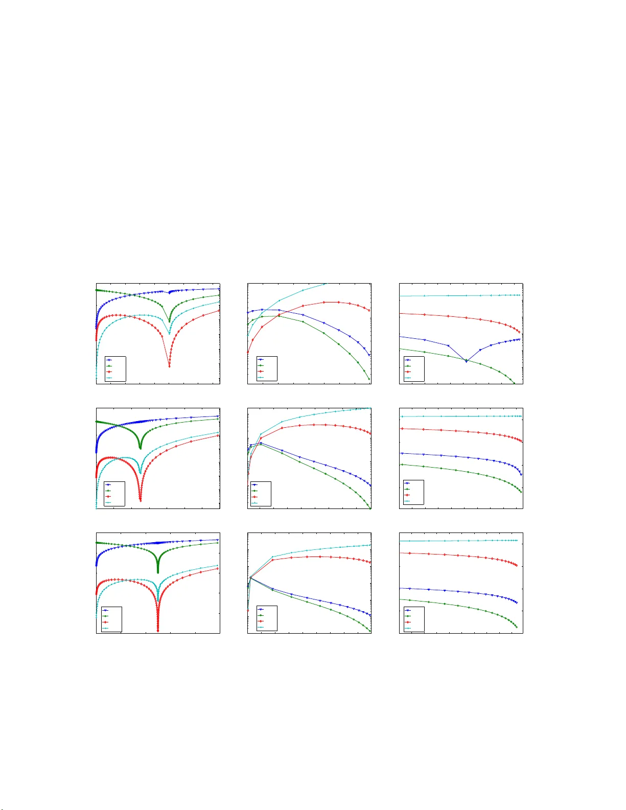
Authors: Suvrit Sra, Dmitrii Karp
The Multiv ariate W atson Distribution: Maxim um-Lik eliho o d Estimatio n and other Asp ects Suvrit Sra ∗ Dmitrii Karp Max Planc k Institute for In t e lligen t Systems Institute of Applied Mathematics T ¨ ubingen, Germany Vladiv ostok, R u ssian F e deration suvrit@tueb ingen.mpg.de dimkrp@gmai l.com Abstract This pap er studies fundamental asp ects of mo delling data using multiv ariate W atson distribu- tions. Alth o ugh t h es e distributions are natural for mo delling axially symmetric data ( i.e., unit vectors where ± x a re equiv alent), for high-dimensions using them can b e difficult—largely b ecause for W atson distributions even basic tasks such as maximum-lik elihoo d are numerically c halleng- ing. T o tackle the numerical difficu lties some app ro ximations hav e b een derived. But these are either gross ly inaccurate in high-dimensions ( Di r e ctional Statistics , Mardia & Jupp. 2000) or when reasonably accurate ( J. Machine L e arning R ese ar ch, W.& C.P., v2 , Bijral et al. , 2007, pp. 35– 42), they lack theoretical justification. W e deriv e asymptotically precise tw o-sided b ounds for t h e maximum-lik elihoo d estimates which lead to new approximati ons. Our approximations are t h e- oretically w ell-defined, numerically accurate, and easy to compute. W e build on our parameter estimation and discuss mixture-mo delling with W atso n d i stributions; here w e uncover a hitherto unknown conn ec tion to the “diametrical clustering” algorithm of Dhillon et al. ( Bioinformatics , 19(13), 2003, pp. 1612–1619). Keyw ords: W atson distribution, Kummer function, Co n fluent hypergeometr ic function, Directional statistics, Diametrical clustering , Spec ia l function, Hyp ergeometric identit y 1 In tro du ction Life on the surface of the unit h yp ersphere is more twisted than you might imag ine : designing e le gant probabilistic mo dels is ea s y but using them is o ften not. This difficult y usually stems fro m the co m- plicated normalising constants asso cia ted with dir ectional distributions. Nevertheless, owing to their powerful modelling ca pabilities, distributions on hyper spheres contin ue finding numerous applications— see e.g., the excellent bo ok Dir e ctional Statistics (Mardia and Jupp, 2 000). A fundamental directional distribution is the von Mises-Fisher (vMF) distribution, which mo dels data concentrated around a mean-direction. But for da ta that have additiona l structure, vMF ca n be ina ppropria te: in particular, for axially symmetric data it is more natural to prefer the (Dimroth- Scheidegger)-W atson distr ibutio n (Ma rdia and Jupp, 2 000; W atson, 19 6 5). And this distributio n is the fo cus of our pap er . Three ma in reasons motiv ate our study of the m ultiv ariate W atson (mW) distribution, namely: (i) it is fundamental to directiona l statistics; (ii) it ha s not r eceived m uc h attention in mo dern data- analysis setups involving high-dimens io nal da ta; and (iii) it provides a theoretical basis to “diametrical clustering”, a pro cedure develop ed for gene-expr ession analysis (Dhillon et al., 20 03). Somewhat s ur prisingly , for high-dimens io nal s ettings, the mW distribution se ems to b e fairly under - studied. One r eason might b e that the traditional do mains of dir ectional statistics are low-dimensional, e.g., circles or spheres . Mo reov er, in low-dimensions n umerical difficulties that are rife in high-dimensions ∗ This wo rk was largely done when the first author was affiliated with the Max Pl anc k Institute for Biological Cybernetics 1 are not so pro nounced. This pap er contributes theor etically and numerically to the study o f the mW distribution. W e hop e that thes e contributions a nd the c onnections we make to es tablished applications help promote wider use of the mW distr ibutio n. 1.1 Related W ork Beyond their use in t ypical a pplications of directional statistics (Mardia and Jupp, 2 000), directional distributions ga ined renewed a ttention in data- mining , where the vMF distribution was first used by (Banerjee et al., 200 3, 200 5), who also derived some ad-ho c parameter estimates; Non ad-ho c pa- rameter estimates for the vMF ca s e were obtained by T anab e et al. (200 7). More rec e nt ly , the W atson distribution was considere d in (Bijra l et al., 2 007) and also in (Sra, 2007). Bijral et al. (2007) used a n approach similar to that o f (Banerjee et al., 20 0 3) to obtain an ad-ho c approximation to the maximum-likelihoo d estimates. W e eliminate the ad-ho c approach and formally derive tight, t wo-sided b ounds which lead to par ameter approximations that are accur ate and efficiently computed. Our der iv atio ns ar e based on car efully exploiting pro p e r ties (several new ones are der ived in this pap er) of the confluen t hyper geometric function, which arises as a pa rt of the no r malisation constan t. Consequently , a large b o dy o f classic a l work on special functions is rela ted to our pa p er. But to av oid detracting from the main message limitations, we relegate highly technical details to the app endix. Another line of related work is base d on mixture- mo delling with dir ectional distributions, esp ecially for hig h-dimensional da ta sets. In (Baner jee e t al., 2005), mixture- mo delling using the Exp ectation Maximisation (E M) a lgorithm for mixture s o f vMFs was related to co sine-similarity based K- means clustering. Sp ecifically , B anerjee et al. (2005) show ed how the co sine based K-mea ns a lg orithm may b e viewed as a limiting ca se of the EM a lgorithm for mixtures o f vMFs. Similar ly , we inv estigate mixture- mo delling using W atson distr ibutio ns, and co nnect a limiting ca se of the corresp onding EM procedur e to a cluster ing algorithm called “ diametrical cluster ing” (Dhillon et al., 2 003). Our viewp oint provides a new in terpretation o f the (discr iminative) diametrical clustering a lgorithm a nd a ls o lends generative semantics to it. Consequently , using a mixture of W atson distributions w e also o btain a clustering pro cedure that can pr ovide be tter clustering results than plain diametric a l clustering alone. 2 Bac kground Let S p − 1 = { x | x ∈ R p , k x k 2 = 1 } b e the ( p − 1)-dimensio nal unit hyperspher e cen tred at the o rigin. W e fo cus on axially s ymmetric vectors, i.e., ± x ∈ S p − 1 are equiv alen t; this is also deno ted by x ∈ P p − 1 , where P p − 1 is the pr o jective hyper plane o f dimension p − 1. A natural choice for mo delling such da ta is the multiv ariate W atson distribution (Mardia a nd Jupp, 2 0 00). This distribution is pa rametrise d by a me an-dir e ction µ ∈ P p − 1 , and a c onc entr ation parameter κ ∈ R ; its pro bability density function is W p ( x ; µ , κ ) = c p ( κ ) e κ ( µ T x ) 2 , x ∈ P p − 1 . (2.1) The normalis ation co nstant c p ( κ ) in (2.1) is given by c p ( κ ) = Γ( p/ 2) 2 π p/ 2 M ( 1 2 , p 2 , κ ) , (2.2) where M is Kummer’s confluen t hypergeometr ic function defined as ((Erd´ elyi et a l., 1953, formula 6.1(1 )) or (Andrews et al., 1999, formula (2.1 .2 )) M ( a, c, κ ) = X j ≥ 0 a j c j κ j j ! , a, c, κ ∈ R , (2.3) and a 0 = 1 , a j = a ( a + 1 ) · · · ( a + j − 1), j ≥ 1, denotes the rising-factorial . Observe that fo r κ > 0, the dens ity concentrates around µ as κ increa s es, wherea s for κ < 0, it concentrates around the gre at circ le orthog o nal to µ . Observe that ( Qµ ) T Qx = µ T x for any orthogona l matrix Q . In particula r for Qµ = µ , µ T ( Qx ) = µ T x ; thus, the W atson density is rotationa lly symmetric ab out µ . 2 2.1 Maxim um Lik eliho o d Estimation W e now cons ide r the bas ic and appa rently simple task of maximum-lik elihoo d parameter estimation for mW distributions: this task turns out to b e sur prisingly difficult. Let x 1 , . . . , x n ∈ P p − 1 be i.i.d. p oints dr awn from W p ( x ; µ , κ ), the W atson density with mean µ and concentration κ . The corresp onding log-likeliho o d is ℓ ( µ , κ ; x 1 , . . . , x n ) = n κ µ T S µ − lo g M (1 / 2 , p/ 2 , κ ) + γ , (2.4) where S = n − 1 P n i =1 x i x T i is the sa mple sc atter matrix , and γ is a constan t ter m that w e c a n ig nore. Maximising (2.4) leads to the following parameter estimates (Mardia and Jupp, 2000, Sec. 10.3.2 ) for the mean vector ˆ µ = s 1 if ˆ κ > 0 , ˆ µ = s p if ˆ κ < 0 , (2.5) where s 1 , . . . , s p are nor malised eigenv ectors ( ∈ P p − 1 ) of the sca tter matrix S corres p o nding to the eigenv alues λ 1 ≥ λ 2 ≥ · · · ≥ λ p . The concentration estima te ˆ κ is obta ined b y solving 1 g ( 1 2 , p 2 ; ˆ κ ) := M ′ ( 1 2 , p 2 , ˆ κ ) M ( 1 2 , p 2 , ˆ κ ) = ˆ µ T S ˆ µ := r (0 ≤ r ≤ 1) , (2.6) where M ′ denotes the der iv ative with resp ect to ˆ κ . Notice that (2.5 ) and (2.6) a re coupled—so we need some wa y to decide whether to so lve g (1 / 2 , p/ 2; ˆ κ ) = λ 1 or to so lve g (1 / 2 , p/ 2; ˆ κ ) = λ p instead. An easy choice is to solve b oth equa tions, and sele c t the s olution that yields a higher log -likelihoo d. Solving these equations is muc h ha rder. One could solve (2.6) using a ro ot-finding metho d (e.g. Newton-Raphso n). But, the s itua tion is not that simple. F or reasons that will soo n become clear , a n out-of-the-b ox r o ot-finding approach can b e unduly s low o r even fraught with numerical p er il, effects that b ecome mo re pr onounced with inc r easing data dimensionality . Let us, therefor e, consider a s lightly mo re gener al e q uation (we also dr o p the accent on κ ): Solv e for κ g ( a, c ; κ ) := M ′ ( a, c ; κ ) M ( a, c ; κ ) = r c > a > 0 , 0 ≤ r ≤ 1 . (2.7) 3 Solving for κ In this section w e present tw o different solutions to (2.7). The first is the “ obvious” metho d based on a Newton-Raphso n r o ot-finder. The s econd metho d is the key num erical contribution of this pap er: a metho d that computes a clo s ed-form approximate solution to (2.7), thereby requiring merely a few floating-p oint op er ations! 3.1 Newton-Raphson Although we establish this fact no t until Section 3.2, supp ose for the moment that (2.7) do es ha ve a solution. F urther, as sume that by bisection o r otherwise, we have bracket ed the ro ot κ to b e within an int erv a l and are thus re ady to in v oke the Newton-Raphson metho d. Starting at κ 0 , Newton-Raphson so lves the equation g ( a, c ; κ ) − r = 0 by iterating κ n +1 = κ n − g ( a, c ; κ n ) − r g ′ ( a, c ; κ n ) , n = 0 , 1 , . . . . (3.1) 1 More precisely , we need λ 1 > λ 2 to ensure a unique m.l. e. for posi tive κ , and λ p − 1 > λ p , for negativ e κ . 3 This iteratio n may b e simplified b y rewriting g ′ ( a, c ; κ ). First no te that g ′ ( a, c ; κ ) = M ′′ ( a, c ; κ ) M ( a, b ; κ ) − M ′ ( a, c ; κ ) M ( a, c ; κ ) 2 , (3.2) then, recall the following tw o identit ies M ′′ ( a, c ; κ ) = a ( a + 1) c ( c + 1) M ( a + 2 , c + 2; κ ); (3.3) M ( a + 2 , c + 2; κ ) = ( c + 1)( − c + κ ) ( a + 1) κ M ( a + 1 , c + 1; κ ) + ( c + 1) c ( a + 1) κ M ( a, c ; κ ) . (3.4) Now, use b oth (3.3) a nd (3.4) to rewrite the der iv ative (3.2) as g ′ ( a, c ; κ ) = (1 − c/κ ) g ( a, c ; κ ) + ( a/ κ ) − ( g ( a, c ; κ )) 2 . (3.5) The main co nsequence of these simplifications is that itera tio n (3.1) can b e implemen ted with only one ev alua tion o f the ratio g ( a, c ; κ n ) = M ′ ( a, c ; κ n ) / M ( a, c ; κ n ). Efficiently computing this ratio is a non-trivial task in itself; an insig ht into this difficult y is offered b y obser v ations in (Gautschi, 1977; Gil et al., 200 7). In the worst case, one may have to compute the numerator and denominator separa tely (using multi-precision floating p oint a r ithmetic), and then divide. Doing so ca n require several million extended precisio n floating p o int op eratio ns , which is very undesirable. 3.2 Closed-form Appro ximation for (2.7) W e now derive t wo-sided b ounds which will lead to a clo s ed-form appr oximation to the so lution o f (2.7). This approximation, while margina lly less accur ate than the one via Newto n-Raphson, should suffice for most uses. Moreov er, it is incompara bly faster to compute as it is in closed- form. Before pro ceeding to the details, let us lo ok at a little history . F or 2–3 dimensional data, or under very restrictive assumptions on κ or r , some a pproximations had b een previo usly obtained (Mardia a nd Jupp, 2000). Due to their restr ictive a s sumptions, these appr oximations have limited a pplicability , esp ecia lly for high-dimensio nal data, where these assumptions are often violated (Baner jee et al., 2005). Re- cently Bijral et al. (2007) follow ed the technique o f Baner jee et al. (2 005) to esse nt ially obtain the ad-ho c approximation (actually particularly for the case a = 1 / 2) B B G ( r ) := cr − a r (1 − r ) + r 2 c (1 − r ) , (3.6) which they observed to be quite a ccurate. How ev er, (3 .6) lacks theoretical justification; other appr oxi- mations were pres e nt ed in (Sra, 200 7), though ag ain only ad-ho c . Below we presen t new appr oximations for κ that ar e theore tica lly w ell-motiv ated and also numer- ically more accurate. K ey to obtaining these approximations are a set o f bounds lo calizing κ , and we present these in a series of theor ems b e low. The pr o ofs are given in the a ppe ndix. 3.2.1 Existence and Uniquenes s The following theorem shows that the function g ( a, c ; κ ) is strictly increa sing. Theorem 3. 1. L et c > a > 0 , and κ ∈ R . Then the function κ → g ( a, c ; κ ) is monotone incr e asing fr om g ( a, c ; −∞ ) = 0 to g ( a, c ; ∞ ) = 1 . Pr o of. Since g ( a, c ; κ ) = ( a/c ) f 1 ( κ ), wher e f µ is defined in (A.11), this theor em is a direct c o nsequence of Theorem A.4. Hence the equation g ( a, c ; κ ) = r ha s a unique s olution for each 0 < r < 1. This solution is nega tive if 0 < r < a /c and p o s itive if a/c < r < 1. Let us now loca lize this so lution to a na rrow interv al by deriving tight b ounds o n it. 4 3.2.2 Bounds on the s olution κ Deriving tight bo unds for κ is key to obtaining o ur new theor etically well-defined n umerical approxi- mations; moreover, these approximations ar e e a sy to co mpute because the bounds are given in closed form. Theorem 3.2. L et the solution to g ( a, c ; κ ) = r b e denote d by κ ( r ) . Consider the fo l lowing thr e e b ounds: ( lower b ound ) L ( r ) = rc − a r (1 − r ) 1 + 1 − r c − a , (3.7) ( b ound ) B ( r ) = rc − a 2 r (1 − r ) 1 + s 1 + 4( c + 1) r (1 − r ) a ( c − a ) ! , (3.8) ( upp er b ound ) U ( r ) = rc − a r (1 − r ) 1 + r a . (3.9) L et c > a > 0 , and κ ( r ) b e the solution (2.7) . Then, we have 1. for a/c < r < 1 , L ( r ) < κ ( r ) < B ( r ) < U ( r ) , (3.10) 2. for 0 < r < a /c , L ( r ) < B ( r ) < κ ( r ) < U ( r ) . (3.11) 3. and if r = a/ c , t hen κ ( r ) = L ( a/c ) = B ( a/ c ) = U ( a/c ) = 0 . Al l thr e e b ounds ( L , B , and U ) ar e also asymptotic al ly pr e cise at r = 0 and r = 1 . Pr o of. The pr o ofs of parts 1 and 2 are g iven in Theor ems A.5 and A.6 (see App endix), re s p ectively . Part 3 is triv ial. It is ea s y to see that lim r → 0 , 1 U ( r ) /L ( r ) = 1, s o fro m inequalities (3.10) a nd (3.1 1), it follows that lim r → 0 , 1 L ( r ) κ ( r ) = lim r → 0 , 1 B ( r ) κ ( r ) = lim r → 0 , 1 U ( r ) κ ( r ) = 1 . More precise a s ymptotic characteriza tions of the appr oximations L , B and U ar e given in sec- tion 3.2.4. 3.2.3 BBG appro ximation Our b ounds ab ove also provide some insight into the prev io us heuristically mo tiv ated κ -approximation B B G ( r ) of Bijr al et al. (200 7) g iven b y (3.6). Sp ecifically , we chec k whether B B G ( r ) satisfies the low er and upper bounds from Theor em 3.2. T o see when B B G ( r ) v iolates the lower b ound, solv e L ( r ) > B B G ( r ) for r to obtain 2 c 2 + a − p (2 c 2 − a )(2 c 2 − a − 8 ac ) 2(2 c 2 − a + c ) < r < 2 c 2 + a + p (2 c 2 − a )(2 c 2 − a − 8 ac ) 2(2 c 2 − a + c ) . F or the W atson case a = 1 / 2; this mea ns that B B G ( r ) violates the low er bound a nd under estimates the solutio n for r ∈ (0 . 1 1 , 0 . 81) if c = 5 ; for r ∈ (0 . 0528 , 0 . 9 04) if c = 1 0 ; for r ∈ (0 . 005 03 , 0 . 99) if c = 100 ; for r ∈ (0 . 00 0500 25 , 0 . 999) if c = 10 00. This fact is a lso reflected in Figure 2. T o see when B B G ( r ) v iolates the upp er bound, so lve B B G ( r ) > U ( r ) for r to obtain r < 2 ac 2 c 2 − a . F or the W atson c a se a = 1 / 2; this means that B B G ( r ) violates the upp er b ound and over estimates the solution fo r r ∈ (0 , 0 . 1) if c = 5; for r ∈ (0 , 0 . 0 5) if c = 10 ; for r ∈ (0 , 0 . 005) if c = 100 ; for r ∈ (0 , 0 . 0005 ) if c = 100 0. What do these violations imply? T he y sho w that a com bination of L ( r ) and U ( r ) is g uaranteed to give a b etter a pproximation than B B G ( r ) for nearly a ll r ∈ (0 , 1 ) except for a very small neighbo urho o d of the p oint where B B G ( r ) in tersects κ ( r ). 5 3.2.4 Asymptotic precision of the appro ximations Let us now lo ok more pr ecisely at how the v arious approximations b ehav e at limiting v alues o f r . There are three points wher e we can compute asymptotics: r = 0, r = a/c , and r = 1. First, we ass ess ho w κ ( r ) itself b ehaves. Theorem 3.3. L et c > a > 0 , r ∈ (0 , 1) ; let κ ( r ) b e the solution to g ( a, c ; κ ) = r . Then, κ ( r ) = − a r + ( c − a − 1) + ( c − a − 1 )(1 + a ) a r + O ( r 2 ) , r → 0 , (3.12) κ ( r ) = r − a c c 2 (1 + c ) a ( c − a ) + c 3 (1 + c ) 2 (2 a − c ) a 2 ( c − a ) 2 ( c + 2) r − a c + O r − a c 2 , r → a c (3.13) κ ( r ) = c − a 1 − r + 1 − a + ( a − 1)( a − c − 1) c − a (1 − r ) + O ((1 − r ) 2 ) , r → 1 . (3.14) This theorem is given in the a pp e ndix with detailed proof as Theo r em A.7. W e ca n compute as ymptotic expansions for the v arious approximations by s tandard Laur ent expa n- sion. F or L ( r ) w e obtain: L ( r ) = − a ( c − a + 1) ( c − a ) r + ( c/ ( c − a ) + c − a ) + O ( r ) , r → 0 , L ( r ) = c 2 ( c + 1) a ( c − a ) ( r − a/c ) + c 3 ( ac − ( c + 1 )( c − a )) a 2 ( c − a ) 2 ( r − a/c ) 2 + O (( r − a/c ) 3 ) , r → a/ c, L ( r ) = c − a 1 − r + (1 − a ) + a ( a − c − 1) c − a (1 − r ) + O ((1 − r ) 2 ) , r → 1 . F or U ( r ) w e get: U ( r ) = − a r + ( c − a − 1) + ( c − a )( a + 1 ) a r + O ( r 2 ) , r → 0 , U ( r ) = c 2 ( c + 1) a ( c − a ) ( r − a/c ) + c 3 (2 ac + a − c 2 ) a 2 ( c − a ) 2 ( r − a/c ) 2 + O (( r − a/ c ) 3 ) , r → a/ c, U ( r ) = (( c/a ) − a + c − 1) 1 − r − (( c/a ) + a ) + O (1 − r ) , r → 1 . F or B ( r ) the expansions ar e: B ( r ) = − a r + a 2 − 2 ac + c 2 − c − 1 c − a + O ( r ) , r → 0 , B ( r ) = c 2 (1 + c ) a ( c − a ) ( r − a/c ) + c 3 (1 + c ) 2 (2 a − c ) a 2 ( c − a ) 2 ( c + 2) ( r − a/c ) 2 + O (( r − a/ c ) 3 ) , r → a/ c, B ( r ) = c − a 1 − r + c + 1 − a 2 a + O (1 − r ) , r → 1 . Finally , for the approximation (3.6) we have the follo wing expansions: B B G ( r ) = − a r + ( c − a ) + O ( r ) , r → 0 , B B G ( r ) = a 2 c ( c − a ) + O ( r − a/c ) , r → a/c, B B G ( r ) = 2 ac − 2 c 2 − 1 2 c (1 − r ) − 2 ac + 1 2 c + O (1 − r ) , r → 1 . W e summar ize the results in T able 1 b elow. 6 T able 1 uses the following terminology: (i) we call an appr oximation f ( r ) to b e inc orr e ct around r = α , if f ( r ) /κ ( r ) → 0 , ∞ as r → α ; (ii) w e say f ( r ) is c orr e ct of or der 1 around r = α , if f ( r ) /κ ( r ) → C such that C 6 = 0 , ∞ as r → α ; (iii) we say f ( r ) is c orr e ct of or der 2 a round r = α if f ( r ) /κ ( r ) = 1 + O ( r − α ) as r → α ; and (iv) f ( r ) is c orr e ct of or der 3 aro und r = α if f ( r ) /κ ( r ) = 1 + O (( r − α ) 2 ) as r → α . No matter ho w we c ount the total ”o r der of cor rectness” it is clear from T able 1 that our appr oxi- mations are sup erio r to that o f (Bijr a l et al., 2 0 07). The table shows that a ctually L ( r ) a nd U ( r ) can b e viewed as three-p oint [2 / 2] Pad ´ e appr oximations to κ ( r ) at r = 0 a nd r = a/c and r = 1 with different orders at different p oints, while B ( r ) is a sp ec ial non-rationa l three p oint approximation with even hig her total order of co ntact. Moreov er, since we not only give the or der o f c orrectnes s but also prove the inequalities, we always know exactly which approximation underestimates κ ( r ) and which ov erestimates κ ( r ). Such information might b e impor tant to some applications. The a pproximation o f (Bijral et al., 20 0 7) is clear ly less precis e and do es not satisfy such inequalities. Also, note that all the a bove facts ar e eq ually true in the W atson case a = 1 / 2. ❳ ❳ ❳ ❳ ❳ ❳ ❳ ❳ ❳ P oint Approx. L ( r ) B ( r ) U ( r ) B B G ( r ) r = 0 Correct of order 1 Correct of order 2 Correct of order 3 Correct of order 2 r = a/c Correct of order 2 Correct of order 3 Correct of order 2 Incorrect r = 1 Correct of order 3 Correct of order 2 Correct of order 1 Correct of order 1 T able 1: Summary of v arious approximations 4 Application to M ixture M o d elling and Clustering Now that w e ha ve shown how to compute maximum-lik eliho o d parameter estimates, w e pr o ceed onto mixtur e-mo del ling for mW distributions. Suppo se w e observe the set X = { x 1 , . . . , x n ∈ P p − 1 } of i.i.d. samples. W e wish to mo del this set using a mixture of K mW distributions. Let W p ( x | µ j , κ j ) be the density of the j -th mixture comp onent, and π j its prior ( 1 ≤ j ≤ K ) – then, for obser v atio n x i we hav e the density f ( x i | µ 1 , κ 1 , . . . , µ K , κ K ) = X K j =1 π j W p ( x i | µ j , κ j ) . The corr esp onding log -likelihoo d for the entire data s et X is g iven by L ( X ; µ 1 , κ 1 , . . . , µ K , κ K ) = X n i =1 log X K j =1 π j W p ( x i | µ j , κ j ) . (4.1) T o ma ximise the log -likelihoo d, we follow a sta ndard Exp ectation Maximis a tion (EM) pro cedur e (Dempster et a l., 1977). T o that end, first bound L fro m b elow as L ( X ; µ 1 , κ 1 , . . . , µ K , κ K ) ≥ X ij β ij log π j W p ( x i | µ j , κ j ) β ij , (4.2) where β ij is the p osterior proba bilit y (for x i , given comp onent j ), and it is defined by the E-Step : β ij = π j W p ( x i | µ j , κ j ) P l π l W p ( x i | µ l , κ l ) . (4.3) 7 Input : X = x 1 , . . . , x n : where each x i ∈ P p − 1 , K : num b er of comp onents Output : Para meter estimates π j , µ j , and κ j , for 1 ≤ j ≤ K Initialise π j , µ j , κ j for 1 ≤ j ≤ K while not c onver ge d do { Perform the E-step of EM } foreac h i and j do Compute β ij using (4.3) (or v ia (4.6) if using hard-assignments) end { Perform the M-step of EM } for j = 1 to K do π j ← 1 n P n i =1 β ij Compute µ j using ( 4.4 ) Compute κ j using (4.5) end end Algorithm 1: EM Algorithm for mixt ure of W atson (moW) Maximising the low er-b ound (4.2) sub ject to µ T j µ j = 1, yields the M-Step : µ j = s j 1 if κ j > 0 , µ j = s j p if κ j < 0 , (4.4) κ j = g − 1 (1 / 2 , p/ 2 , r j ) , where r j = µ T j S j µ j , (4.5) π j = 1 n X i β ij , where s j i denotes the eige nv e ctor cor resp onding to e ig env alue λ i (where λ 1 ≥ · · · ≥ λ p ) o f the weighte d- sc att er matrix: S j = 1 P i β ij X i β ij x i x T i . Now we can iterate b etw een (4.3), (4.4) and (4.5) to o btain an EM a lgorithm. Pseudo-co de for suc h a pro cedure is shown b elow as Algorithm 1. Note: Hard As signme nts. W e note that a s usua l, to reduce the computatio na l burde n, we can replace can E-s tep (4 .3) by the standard har d-assignment heur istic: β ij = ( 1 , if j = a r gmax j ′ log π j ′ + log W p ( x i | µ j ′ , κ j ′ ) , 0 , o ther wise . (4.6) The corr esp onding M -Step also simplifies cons iderably . Such hard- assignments maximize a low er- bo und on the incomplete log-likeliho o d, and yield p artitional-clustering algorithms (in fa c t, we show exp erimental results in Sec tion 5.2 where we cluster data using a pa r titional-cluster ing algor ithm based on this hard-a ssignment heur istic). 4.1 Diametrical Clustering W e now turn to the diametr ical clustering algo rithm of Dhillon et al. (200 3), and s how that it is mere ly a specia l case of the mixture -mo del describ ed ab ov e. Diametrical clustering is motiv ated by the need to group tog ether corr elated and anti-correlated data p oints (see Figure 1 fo r an illus tration). F or data normalised to have unit euclidean nor m, suc h clustering trea ts diametric al ly oppo site p oints equiv alen tly . In other words, x lies on the pro jective plane. Therefore, a natur al question is whether diametr ical clustering is related to W atson distributio ns , and if so, how? The answer to this question will b ecome a pparent once we reca ll the diametrical clustering algor ithm (shown as Alg orithm 2) of (Dhillon et al., 20 0 3). In Algorithm 2 we have labelled the “E-Step” and the “M-Step” . These tw o steps are s implified instances of the E -step (4.3) (alter natively 4.6) and 8 Input : X = { x 1 , . . . , x n : x i ∈ P p − 1 } , K : num ber of clusters Output : A partition {X j : 1 ≤ j ≤ K } of X , and centroids µ j Initialise µ j for 1 ≤ j ≤ K while not conv erged do E-step: Set X j ← ∅ for 1 ≤ j ≤ K for i = 1 to n do X j ← X j ∪ { x i } where j = argmax 1 ≤ h ≤ K ( x T i µ h ) 2 end M-step: for j = 1 to K do A j = P x i ∈X j x i x T i µ j ← A j µ j / k A j µ j k end end Algorithm 2: D iametrical Clustering −1 −0.5 0 0.5 1 −1 −0.5 0 0.5 1 −1 −0.5 0 0.5 1 −1 −0.5 0 0.5 1 −1 −0.5 0 0.5 1 −1 −0.5 0 0.5 1 Figure 1: The left panel shows a xially symmetric data that has tw o c lus ters (centroids are indicated by ’+’ a nd ’x ’). The middle and right panel shows cluster ing yielded by (Euclidea n) K -means (note that the centroids fail to lie on the cir cle in this case) with K = 2 and K = 4, resp ectively . Diametrical clustering recovers the tr ue cluster s in the left panel. M-step (4.4). T o s ee why , consider the E-step (4.3). If κ j → ∞ , then for each i , the co rresp onding po sterior probabilities β ij → { 0 , 1 } ; the particular β ij that tends to 1 is the one for which ( µ T j x i ) 2 is maximised – this is pr ecisely the choice used in the E - step of Algorithm 2. With bina ry v alue s for β ij , the M-Step (4.4) also reduces to the version follow ed by Algo r ithm 2 . An a lternative, per ha ps b etter view is obtained b y reg arding dia metr ical clustering as a specia l case o f mixture-mo delling wher e a hard-assig nment rule is used. Now, if all mixture compo ne nts hav e the same, p ositive concentration par ameter κ , then while computing β ij via (4.6) we may ignor e κ altogether, which reduce s Alg orithm 1 to Algor ithm 2. Given this interpretation o f diametrical clustering, it is natur a l to exp ect that the additiona l mo d- elling p ow er offered by mixtures o f W atson distributions might lead to b etter clus tering. This is indeed the case , as indicated by some of our exp er iment s in Section 5.2 b elow, w he r e we s how that mer ely including the c oncentration para meter κ can lead to improv ed c lus tering accur acies, or to cluster s with higher quality (in a sens e that will b e made mor e precise b elow). 5 Exp erimen ts W e now come to numerical results to asses s the metho ds presented. W e divide our exp eriments int o tw o groups. The fir st group co mprises num erical r esults that illustra te accurac y of our approximation to κ . The se c ond gro up suppo rts our cla im that the extra modelling pow er offere d b y moWs also tra nslates 9 int o b etter clustering r esults. 5.1 Estimating κ W e show tw o representativ e exp er iment s to illustrate the a ccuracy of o ur approximations. The first set ( § 5.1.1) compare s our approximation with tha t of Bijra l et al. (2007), as given by (3.6). This set considers the W atson case, namely a = 1 / 2 and v arying dimensionality c = p/ 2 . The seco nd set ( § 5.1 .2) of exper iments shows a sampling of results for a few v alues of c and κ as the para meter a is v a ried. This set illustrates how well o ur approximations b ehave for the general nonlinear equation (2.7). 5.1.1 Comparison with the BBG appro ximation for the W atson case Here w e fix a = 1 / 2 , and v ar y c on an exp o nent ially spaced g r id r anging from c = 1 0 to c = 10 4 . F or each v a lue of c , we gener ate g eometrically spaced v a lues of the “ true” κ ∗ in the r ange [ − 200 c, 20 0 c ]. F or each choice of κ ∗ pick e d within this rang e, we compute the r atio r = g (1 / 2 , c, κ ∗ ) (using Ma thema tica for high precision). Then, given a = 1 / 2, c , and r , we e stimate κ ∗ by solving κ ≈ g − 1 (1 / 2 , c, r ) using B B G ( r ), L ( r ), B ( r ), and U ( r ), giv en by (3.6), (3.7), (3 .8), and (3.9), res pe c tively . 0 0.01 0.02 0.03 0.04 0.05 0.06 0.07 0.08 10 −7 10 −6 10 −5 10 −4 10 −3 10 −2 10 −1 r Relative error: | κ − κ * |/| κ * | Approximation BBG(r) versus ours, c = 10 (r ≈ 0) BBG(r) L(r) B(r) U(r) 0.1 0.2 0.3 0.4 0.5 0.6 0.7 0.8 0.9 10 −3 10 −2 10 −1 10 0 r Relative error: | κ − κ * |/| κ * | Approximation BBG(r) versus ours, c = 10 BBG(r) L(r) B(r) U(r) 0.9 0.91 0.92 0.93 0.94 0.95 0.96 0.97 0.98 0.99 10 −4 10 −3 10 −2 10 −1 10 0 10 1 r Relative error: | κ − κ * |/| κ * | Approximation BBG(r) versus ours, c = 10 (r ≈ 1) BBG(r) L(r) B(r) U(r) 0 0.002 0.004 0.006 0.008 0.01 0.012 0.014 10 −8 10 −7 10 −6 10 −5 10 −4 10 −3 10 −2 10 −1 r Relative error: | κ − κ * |/| κ * | Approximation BBG(r) versus ours, c = 100 (r ≈ 0) BBG(r) L(r) B(r) U(r) 0.1 0.2 0.3 0.4 0.5 0.6 0.7 0.8 0.9 10 −3 10 −2 10 −1 10 0 r Relative error: | κ − κ * |/| κ * | Approximation BBG(r) versus ours, c = 100 BBG(r) L(r) B(r) U(r) 0.9 0.91 0.92 0.93 0.94 0.95 0.96 0.97 0.98 0.99 10 −6 10 −4 10 −2 10 0 r Relative error: | κ − κ * |/| κ * | Approximation BBG(r) versus ours, c = 100 (r ≈ 1) BBG(r) L(r) B(r) U(r) 0 0.2 0.4 0.6 0.8 1 x 10 −3 10 −12 10 −10 10 −8 10 −6 10 −4 10 −2 r Relative error: | κ − κ * |/| κ * | Approximation BBG(r) versus ours, c = 1000 (r ≈ 0) BBG(r) L(r) B(r) U(r) 0 0.1 0.2 0.3 0.4 0.5 0.6 0.7 0.8 0.9 10 −5 10 −4 10 −3 10 −2 10 −1 10 0 10 1 r Relative error: | κ − κ * |/| κ * | Approximation BBG(r) versus ours, c = 1000 BBG(r) L(r) B(r) U(r) 0.9 0.91 0.92 0.93 0.94 0.95 0.96 0.97 0.98 0.99 10 −8 10 −6 10 −4 10 −2 10 0 r Relative error: | κ − κ * |/| κ * | Approximation BBG(r) versus ours, c = 1000 (r ≈ 1) BBG(r) L(r) B(r) U(r) Figure 2: Relative error s | ˆ κ − κ ∗ | / | κ ∗ | of B B G ( r ), L ( r ), B ( r ), and U ( r ) for c ∈ { 10 , 10 0 , 1 000 , 10000 } as r v ar ies b etw een (0 , 1). The left column shows errors for “small” r (i.e., r clo se to 0), the middle column shows e r rors for “ mid- r ange” r , a nd the la s t c o lumn shows er rors for the “ high” range ( r ≈ 1 ). Figure 2 shows the res ults of co mputing these a pproximations. Two p oints ar e immediate from 10 the plots: (i) appr oximation L ( r ) is more accurate than B B G ( r ) acros s a lmost the whole r a nge of dimensions and r v alues; and (ii) for small r , B B G ( r ) can b e mo re a ccurate than L ( r ), but in this c a se bo th U ( r ) and B ( r ) are muc h more accurate. 5.1.2 Comparisons of the appro ximation for fi xed c and v arying a 0 0.2 0.4 0.6 0.8 1 10 −4 10 −3 10 −2 10 −1 10 0 r (varies montonically with a) Relative error: | κ − κ * |/| κ * | Approximation BBG(r) versus ours, κ =2, c = 10, a ∈ [.01c, .99c] BBG(r) L(r) B(r) U(r) 0.5 0.6 0.7 0.8 0.9 1 10 −5 10 −4 10 −3 10 −2 10 −1 10 0 r (varies montonically with a) Relative error: | κ − κ * |/| κ * | Approximation BBG(r) versus ours, κ =200, c = 100, a ∈ [.01c, .99c] BBG(r) L(r) B(r) U(r) 0 0.2 0.4 0.6 0.8 1 10 −6 10 −5 10 −4 10 −3 r (varies montonically with a) Relative error: | κ − κ * |/| κ * | Approximation BBG(r) versus ours, κ =500, c = 1000, a ∈ [.01c, .99c] BBG(r) L(r) B(r) U(r) 0.4 0.5 0.6 0.7 0.8 0.9 1 10 −6 10 −5 10 −4 10 −3 10 −2 r (varies montonically with a) Relative error: | κ − κ * |/| κ * | Approximation BBG(r) versus ours, κ =1500, c = 1000, a ∈ [.01c, .99c] BBG(r) L(r) B(r) U(r) Figure 3: Relative erro rs of B B G ( r ), L ( r ), B ( r ), and U ( r ) for differen t sets of c and κ v alues, as a is v arie d fr om 0 . 01 c to 0 . 99 c . In our next set of exp eriments, we chose a few v alues of c a nd κ (see Figure 3), and v a r ied a linea rly to lie in the range [0 . 01 c, 0 . 9 9 c ]. Fig ure 3 rep or ts the relative e rror s of approximation incurred by the v ario us a ppr oximations. F rom the plots it is clear that one of L ( r ), B ( r ), or U ( r ) alwa ys yields results more ac c ur ate than B B G ( r ). The v arious r esults sug gest the following ro ugh rule-o f-th umb: prefer U ( r ) for 0 < r < a/ (2 c ), prefer B ( r ) for a / (2 c ) ≤ r < 2 a/ √ c and prefer L ( r ) for 2 a / √ c ≤ r < 1. 5.2 Clustering using mW distributions Now we turn to our se c o nd set of exp eriments. Below we show r esults of tw o ex p er iments: (i) with synthetic data, w her e a desired “true- clustering” is known; and (ii) with ge ne expressio n data for which previously axially symmetr ic clus ter s hav e b een considered. F or b oth our exp eriments, we compare mo W (Algo rithm 1 with (4.6) fo r the E -step) against the diametrical clustering pr o cedure of Dhillon et al. (2003). The key aim o f the exp eriments is to show that the ex tr a mo de lling p ow er o ffered by a mixture of mW distributions ca n provide clustering results better than plain diametrical clustering. 11 T able 2: Percent ages of accurately clustered points for dia metrical c lus tering vs . moW (ov er 10 runs ). Since this is simu lated data, we knew the cluster labels. The accura cy is then computed by ma tching the pr edicted lab els with the k nown ones. In line with the theory , with increasing co ncentration the mo delling p ow er o ffered by moW shows a c lear adv antage over o rdinary diametrical cluster ing. κ 2 Diametrical (avg/best/w orst)-% moW (avg/best/w orst)-% 3 52.65 / 56.50 / 51.50 51.65 / 53.50 / 50.50 10 52.75 / 56.00 / 50.50 54.10 / 57.00 / 50.00 20 57.60 / 64.00 / 51.50 74.45 / 87.00 / 63.50 50 66.00 / 78.50 / 50.00 99.50 / 99.50 / 99.50 100 71.20 / 81.00 / 55.00 100.00 / 100.00 / 100.00 5.2.1 Syn thetic data W e genera ted data that merely ex hibit axial s ymmetry a nd have v arying degre e s of co nc e ntration aro und given mea n directions. Since bo th the diametrical method as well as moW mo del axial symmetry they can be fair ly compared on this data. The distinction comes, how ever, wher e moW fur ther mo dels con- centration (via κ ), and in case the g enerated data is sufficient ly co ncentrated, this mo delling translates int o empirically superio r performa nce. Natur ally , to avoid unfairly skewing results in fa vour of moW, we do not co mpare it a gainst diametrica l clustering o n synthetic da ta sampled from a mixture of mW distributions as moW explicitly optimises such a model. F or our data gene r ation we need to sa mple p oints from W p ( κ, µ ), for whic h we inv oke a simplified version o f the p ow erful Gibbs sampler of (Hoff, 2009) that can sim ulate Bing ham-von Mise s -Fisher distributions. W e no te he r e that Bingham distribution is parametrised by a matrix A , and to use it for sampling W atson dis tributions, we mere ly nee d to rea lise that A = κ µµ T . With the sa mpling co de in hand, we generate synthetic data sets with v arying concentration as follows. First, t w o random unit vectors µ 1 , µ 2 ∈ P 29 are selected. Then, we fix κ 1 = 3 a nd sa mple 2 00 po ints from W 3 ( κ 1 , µ 1 ). Next, we v ary κ 2 in the set { 3 , 1 0 , 2 0 , 5 0 , 1 00 } , a nd generate 200 p oints for each v alue of κ 2 by sampling from W p ( κ 2 , µ 2 ). Finally , b y mixing the κ 1 comp onent with eac h of the five κ 2 comp onents we obtain fiv e datas ets X t (1 ≤ t ≤ 5). Each o f these five datasets is then cluster ed into tw o clusters, us ing mo W and diametrical clustering. Both algor ithms are run ten times each to smo oth out the e ffect of ra ndo m initializations. T able 2 shows the results o f clustering by displaying the accuracy which measur e s the p ercentage o f data p o ints that were a ssigned to the “tr ue” clusters (i.e., the true co mp onents in the mixture). The a ccuracies stro ngly indicate that explicit mo delling of co ncentration leads to b etter clustering a s κ 2 increases. In other words, lar ger κ 2 makes p o ints fro m the second clus ter more co ncentrated ar ound ± µ 2 , thereby allowing easier separatio n b etw een the clusters. 5.2.2 Real Data W e now compar e cluster ing r e sults of moW with those of dia metrical clustering on thr ee gene micro array datasets that were als o used in the origina l dia metrical clustering pap er (Dhillon et a l., 2003). These datasets are: (i) Human Fibrobla sts (Iyer et a l., 1999); (ii) Y est Cell Cycle (Sp ellman et a l., 19 98); a nd (iii) Rosetta yeast (Hughes et al., 200 0). The resp ective matrix sizes that w e used were: (i) 517 × 12; (ii) 696 × 82; a nd (iii) 90 0 × 300 (these 900 genes were randomly selected from the o riginal 5245 ). Since we do not hav e ground- tr uth clusterings for these datasets, we v alidate our results using int ernal measures. Sp ecifically , we compute tw o sco r es: homo geneity and sep ar ation , which ar e defined below by H avg and S avg , resp ectively . Let X j ⊂ X denote cluster j ; then we define H avg = 1 n K X j =1 X x i ∈X j ( x T i µ j ) 2 , (5.1) S avg = 1 P j 6 = l |X j ||X l | X j 6 = l |X j ||X l | min( µ T j µ l , − µ T j µ l ) . (5.2) 12 T able 3: Clustering accuracy on gene-expr ession datasets (over 10 runs). Noticeable difference s (i.e., > 0 . 02) b etw e e n the a lgorithms are highlighted in b o ld. Method Diametrical (avg/best/w orst) moW (avg/best/w orst) Y east-4 Homogeneit y 0.38 / 0.38 / 0.38 0.37 / 0.37 / 0.37 Separation -0.00 / - 0.23 / 0.24 -0.04 / -0.23 / 0.20 Y east-6 Homogeneit y 0.41 / 0.41 / 0.40 0.41 / 0.41 / 0.40 Separation -0.06 / - 0.15 / 0.14 -0.07 / -0.20 / 0.13 Rosetta-2 Homogeneit y 0.16 / 0.17 / 0.16 0.16 / 0.17 / 0.16 Separation 0.24 / 0.08 / 0.28 -0.20 / -0.28 / 0.09 Rosetta-4 Homogeneit y 0.23 / 0.23 / 0.23 0.23 / 0.23 / 0.23 Separation -0.01 / - 0.08 / 0.16 -0.03 / -0.09 / 0.12 Fibroblast-2 Homogeneit y 0.70 / 0.70 / 0.70 0.70 / 0.70 / 0.70 Separation 0.26 / -0.65 / 0.65 -0.01 / -0.65 / 0.65 Fibroblast-5 Homogeneit y 0.78 / 0.78 / 0.78 0.76 / 0.76 / 0.75 Separation -0.05 / - 0.28 / 0.40 -0.12 / -0.30 / 0.35 W e note a slight departure from the sta ndard in our definitions ab ove. In (5.1 ), instead o f summing ov er x T i µ j , we sum ov er their squa res, while in (5.2), instead of µ T j µ l , we use min( µ T j µ l , − µ T j µ l ) because for us + µ j and − µ j represent the same cluster. W e note that diametrical clustering optimises precisely the criterio n (5.1), and is th us fav oured by our criterio n. Higher v alues of H avg mean that the clusters hav e higher intra-cluster cohe s iveness, and th us ar e “ be tter” cluster s. In contrast, low er v a lues of S avg mean that the in ter-cluster dissimilar ity is high, i.e., b etter sepa rated clusters. T able 3 shows results yielded by diametrica l clustering a nd moW on the three differen t gene datasets. F or ea ch da taset, we show r esults for tw o v alues o f K . The H avg v alues indicate that moW yields clusters having appr oximately the same intra-cluster cohesiveness a s diametr ical. How ev er, moW attains b etter int er-cluster separa tion a s it more freq uent ly leads to lower S avg v alues. 6 Conclusions W e studied the multiv ariate W atson distribution, a fundamental tool for modelling axia lly symmetric data. W e solv ed the difficult no nlinear eq uations that arise in maximum-likelihoo d parameter estima- tion. In high-dimensio ns these equations p os e severe numerical challenges. W e derived tig ht tw o -sided bo unds that led to approximate solutions to these equa tions; we also showed our so lutions to b e accura te. W e applied our results to mixture-mo delling with W atson dis tributions and consequently uncovered a connection to the diametrical clustering algor ithm of (Dhillon et a l., 20 0 3). Our e x p e r iments show e d that fo r clustering axia lly symmetric data, the additional mo delling p ow er o ffered by mixtures of W at- son distr ibutions can lead to b etter c lustering. F urther r efinements to the clustering pro cedur e, as w ell as other applications o f W atson mixtures in high- dimensional settings is left as a tas k for the future. Ac kno wledgemen ts The first author thanks Prateek Ja in for initial disc ussions rela ted to W atson distributions. The seco nd author acknowledges supp or t of the Russia n Ba sic Research F und (grant 11-0 1-00 038-a ). 13 References References Andrews, G. E., Askey , R ., Roy , R., 1999. Sp ecial functions. Cambridge Universit y Press. Banerjee, A., D hillon, I. S ., Ghosh, J., Sra, S., 2003. Generative mo del-based clustering of directional data. In: Pro ceedings of The Ninth ACM SI GKDD In ternational Conference on Kno wledge Disco very and Data Mining(KDD-2003). p p . 19–28. Banerjee, A., Dhillon, I. S., Ghosh, J., Sra, S., S ep 2005. Clustering on th e U nit Hyp ersph ere u sing von Mises- Fisher Distributions. J. Mac hine Learning R esearc h 6, 1345–138 2. Bijral, A., Breitenbac h, M., Grudic, G. Z., 2007. Mixture of W atson Distributions: A Generative Mod el for Hyp erspherical Embedd ings. In: Artificial I ntelli gence and Statistics (AIST A TS 2007). pp. 35–42. Cuyt, A., P etersen, V. B., V erdonk , B., W aadeland, H., Jones, W. B., 2008. Handb o ok of Contin ued F ractions for Sp ecial F un ctions. Springer. Dempster, A., Laird, N., Rub in, D., 1977. Maxim um Likelihood from Incomplete Data V ia the EM Algorithm. Journal of the R oy al Statistical So ciet y 39. Dhillon, I. S., Marcotte, E. M., R oshan, U., 2003. Diametrical clustering for identif ying anti-correlated gene clusters. Bioinformatics 19 (13), 1612–1619. Erd´ elyi, A., Magnus, W., Oberhett inger, F., T rico mi, F. G., 1953. Higher transcendental functions. V ol. 1. McGra w Hill. Gautsc hi, W ., 1977. Anomalous Conv ergence of a Con tinued F raction for Ratios of Kummer F unctions. Math- ematics of Computation 31 (140), 994–999. Gil, A., S egura, J., T emme, N . M., 2007. N u merical Methods for Sp ecial F un ct ions. Cambridge Universit y Press. M.O. Gonzalez, Classical Complex Analysis (Pure and App lied Mathematics), CRC Press, 1991. A. Hurwitz, R. Couran t, V orlesungen ¨ u b er allgemeine F uktionentheorie un d Elliptisc he F uktionen, Second Edi- tion, V erlag von Julius Springer, Berlin, 1925. R. L. Graham, D. E. Knuth, and O . Patashnik, 1998. Concrete Mathematics. Ad dison W esley . Hoff, P . D., 2009. Simulatio n of the Matrix Bingham–v on Mises–Fisher D istribution, W ith Applications to Multiv ariate and Relational D ata. Journal of Comput ational and Graphical Statistics 18 ( 2), 438–456. Hughes, T. R., Marton, M. J., Jones, A. R., Rob erts, C. J., Stoughton, R., A rmour, C. D., Bennett, H. A., Coffey , E., Dai, H., Shoemaker, D. D., Gac h otte, D., Chakraburtty , K ., Simon, J., Bard, M., F riend, S . H., 2000. F unctional discov ery via a compen dium of expression profiles. Cell 102, 109–126. Iyer, V. R ., Eisen, M. B., Ross, D. T., Sch uler, G., Mo ore, T., Lee, J. C. F., T ren t, J. M., Staudt, L. M., Hu dson, J., Boguski, M. S., Lashk ari, D., Sh alon, D., Botstein, D., Bro wn, P . O., 1999. The T ranscriptional Program in the Resp onse of Human Fibroblasts to Serum. Science 283 (5398), 83–87. Karp, D., 2011. T ur´ an’s inequalit y for the Kummer function of th e p hase shift of tw o parameters. Journal of Mathematical Sciences 178 (2), 178–186. Karp, D., Sitnik , S. M., 2010. Log-conv exit y and log-conca vity of hypergeometric-like functions. Journal of Mathematical A n alysis and App lications 364, 384–394 . Mardia, K. V ., Jupp, P ., 2000. Directional Statistics, 2nd Edition. John Wiley & Sons. Sp ellman, P . T., Sherlock, G., Zhang, M., Iyer, V . R., Anders, K., Eisen, M., Bro wn, P . O., Botstein, D ., F utcher, B., 1998. Comprehensiv e identification of cell cycle regulated gene of the yeast S accharo myces Cerevisia by microarra y hybridization. Mol. Bio. Cell 9, 3273–3297. Sra, S., 2007. Matrix Nearness Problems in Data Mining. Ph.D. thesis, Un iv. of T exas at A ustin. T anabe, A., F uk u mizu, K., Ob a, S., T ak enouchi, T., Ishii, S., 2007. P arameter estimation for von Mises-Fisher distributions. Computational Statistics 22 (1), 145–15 7. W atson, G. S., 1965. Equatorial distribut ions on a sphere. Biometrik a 52 (1-2), 193–201. 14 A Mathematical Details This app endix includes mathematical details supp or ting the technical ma terial of the main text. While many of the facts are classic knowledge, s ome migh t b e found only in sp ecialised literature. Thus, we hav e erred on the side of including to o m uch ra ther than too little. A.1 Hyp ergeometric functions Hyper geometric functions pro vide one of the ric hest classes of functions in a nalysis. Indeed, any series with ratio of neighbour ing ter ms equal to a rationa l function o f the summation index is a constant m ultiple of the gener alise d hyp er ge ometric function p F q defined by the p ow er-serie s p F q ( a 1 , . . . , a p ; c 1 , . . . , c q ; z ) = X k ≥ 0 a 1 k · · · a p k c 1 k · · · c q k z k k ! , (A.1) where a k = a ( a + 1) . . . ( a + k − 1) is the rising factorial (often a lso denoted by the Pochhammer sy mbol ( a ) k ). Hyp erg e o metric functions arise naturally as solutions to cer ta in differen tial equations; for a gentle int ro duction to hyper geometric functions we refer the reader to (Graha m et al., 1998), while for a mor e adv ance d trea tment the reader may find (Andrew s et al., 1999) v alua ble . In this pa p er, we restrict our attention to Kummer’s confluent hyper geometric function: 1 F 1 , w hich is also denoted a s M . Moreov er, we limit our attention to the case of r eal v alued arg uments. A.1.1 Some useful ide n tities for M ( a, c , x ) W e list below some ident ities for M that w e will need for our a nalysis. T o ea se the notational burden, we also use the sho r thand M i ≡ M ( a + i, c + i, x ); e .g ., M 0 ≡ M ( a, c, x ). d n dx n M 0 = a n c n M n . (A.2) M 1 = c (1 − c + x ) ax M 0 + c ( c − 1) ax M − 1 . (A.3) ( c − a ) M ( a + 1 , c + 2 , x ) = ( c + 1) M 1 − ( a + 1) M 2 (A.4) ( c − a ) xM ( a + 2 , c + 3 , x ) = ( c + 1)( c + 2)[ M 2 − M 1 ]; (A.5) ( a + 1) xM 2 = ( c + 1 )( x − c ) M 1 + c ( c + 1 ) M 0 (A.6) xM ( a + 2 , c + 3 , x ) = ( c + 2)[ M 2 − M ( a + 1 , c + 2 , x )] , (A.7) Ident ity (A.2) follows inductiv ely; (A.3) fro m (Cuyt et al., 2 008, 1 6 .1.9c); (A.4) from (Erd´ elyi et al., 1953, formula 6.4 (4 )); (A.5) on combining (Erd´ elyi et a l., 1953, formula 6.4(5 )) with (Er d´ elyi et al., 1953, formula 6 .4(4)); (A.6) from (A.3) by replacing c → c + 1, a → a + 1 ; and (A.7) from (Erd´ elyi et al., 1953, formula 6.4(5)). Now we build on the ab ove identit ies to introduce a technical but crucia l lemma. Lemma A.1. The fol lowing identity hold s for the Ku mmer function: M 2 1 − M 2 M 0 = ( c − a ) x c + 1 1 c + 1 M ( a + 1 , c + 2 , x ) 2 − 1 c + 2 M ( a + 2 , c + 3 , x ) M ( a, c + 1 , x ) + 1 c ( c + 1) M ( a + 1 , c + 2 , x ) M ( a + 2 , c + 2 , x ) . (A.8) 15 Pr o of. Application of (A.4) a nd (A.5) yields after collecting terms 1 c + 1 M ( a + 1 , c + 2 , x ) 2 − 1 c + 2 M ( a + 2 , c + 3 , x ) M ( a, c + 1 , x ) + 1 c ( c + 1) M ( a + 1 , c + 2 , x ) M 2 = a ( a + 1) c ( c − a ) 2 M 2 2 − c ( c + 1) ( c − a ) 2 x M 2 M 0 − ( c + 1)( a − x ) ( c − a ) 2 x M 2 1 + c ( c + 1) ( c − a ) 2 x M 1 M 0 + ac ( c + 1 ) − x ( a + c + 2 ac ) ( c − a ) 2 cx M 2 M 1 . (A.9) Application of this formula allows us to write the differenc e betw een the left-hand and rig ht-hand sides of (A.8) as lhs − r hs = cM 1 − aM 2 c ( c + 1)( c − a ) x ( a + 1) M 2 − ( c + 1 )( x − c ) M 1 − c ( c + 1 ) M 0 = 0 , where the equality to 0 is due to (A.6 ). A.2 The Kummer ratio The central ob ject of study in this paper is the Ku mmer-r atio : g ( x ) = g ( a, c ; x ) := M ′ ( a, c, x ) M ( a, c, x ) = a c M ( a + 1 , c + 1 , x ) M ( a, c, x ) . (A.10 ) This ratio satisfies many fascinating prop erties; but of necessity , we must conten t ours elves with only the essential pr op erties. In particula r, o ur analys is fo cuses o n the fo llowing: (i) proving that g is monotonic, and ther eby inv ertible; and (ii) obtaining b o unds o n the ro ot of g ( x ) − r = 0. In the sequel, it will b e useful to use the slig htly more gener al function f µ ( x ) := M ( a + µ, c + µ, x ) M ( a, c, x ) , µ > 0 , (A.11) so that g ( x ) = ( a/ c ) f 1 ( x ). Befor e proving monotonicity of g , we derive tw o useful lemmas. Lemma A.2 (Lo g-conv exity) . L et c > a > 0 and x ≥ 0 . Then the function µ 7→ Γ( a + µ ) Γ( c + µ ) M ( a + µ, c + µ, x ) = ∞ X k =0 Γ( a + µ + k ) Γ( c + µ + k ) x k k ! =: h a,c ( µ ; x ) is strictly lo g-c onvex on [0 , ∞ ) (n ote that h is a function of µ ). Pr o of. W rite the pow er-series e x pansion in x for h a,c ( µ ; x ) a s h a,c ( µ ; x ) = ∞ X k =0 h k ( a, c, µ ) x k k ! , h k ( a, c, µ ) = Γ( a + µ + k ) Γ( c + µ + k ) . Since log- conv exit y is additive it is sufficien t to prove that µ 7→ h k ( a, c, µ ) is lo g -conv ex. F or this we compute the seco nd-deriv a tive ∂ 2 ∂ µ 2 log h k ( a, c, µ ) = ψ ′ ( a + µ + k ) − ψ ′ ( c + µ + k ) , where ψ is the logarithmic der iv ative of the gamma function. W e need to show that this expr e ssion is po sitive when c > a > 0, k ≥ 0 and µ ≥ 0 . According to the Gauss formula (Andrews et a l., 1999, Theorem 1.6.1 ) ψ ( x ) = ∞ Z 0 e − t t − e − tx 1 − e − t dt, 16 so that ψ ′′ ( x ) = − ∞ Z 0 t 2 e − tx 1 − e − t dt < 0 . Hence the function ψ ′ ( x ) is decreas ing and our cla im fo llows. Lemma A.3. L et c > a > 0 , and x ≥ 0 . Then the function µ 7→ Γ( a + µ ) Γ( c + µ ) M ( c − a, c + µ, x ) =: ˆ h a,c ( µ ; x ) is strictly lo g-c onvex on [0 , ∞ ) . Pr o of. Using pre c isely the same arg ument as in the pro of of L e mma A.2 we see that µ 7→ Γ( a + µ ) / Γ( c + µ ) is lo g -conv ex. Next, the log-conv exity of µ 7→ M ( c − a ; c + µ ; x ) has b een prov ed by many authors (see, for instance, Karp and Sitnik (201 0) and refere nces there in). Thus multiplicativit y of log-conv exity completes the pro o f. With these tw o lemmas in hand we ar e r eady to prov e the fir st main theorem. Theorem A.4 (Mono tonicity) . L et c > a > 0 . The funct ion x 7→ f µ ( x ) is monotone incr e asing on ( −∞ , ∞ ) , with f µ ( −∞ ) = 0 and f µ ( ∞ ) = Γ( c + µ )Γ( a ) / Γ( c )Γ( a + µ ) . Pr o of. W e divide the pro of in to tw o c a ses: (i) x ≥ 0 , and (ii) x < 0. Case i: Let x ≥ 0. It fo llows from (A.2) that d dx M ( a, c, x ) = a c M ( a + 1 , c + 1 , x ) , whereby (using our co mpa ct no tation) we have M 2 0 f ′ µ ( x ) = a + µ c + µ M µ +1 M 0 − a c M µ M 1 . W e need to show that the ab ove expr ession is p ositive, which amo unts to showing a + µ c + µ M µ +1 M µ > a c M 1 M 0 , (A.12) or equiv a lently [Γ( a + µ + 1 ) / Γ( c + µ + 1)] M µ +1 [Γ( a + µ ) / Γ( c + µ )] M µ > [Γ( a + 1) / Γ( c + 1)] M 1 [Γ( a ) / Γ( c )] M 0 . The last inequality follo ws from Lemma A.2. T o see how, r ecall that if µ 7→ h ( µ ) is log- c onv ex, then the function µ 7→ h ( µ + δ ) /h ( µ ) is increas ing 2 for each fixed δ > 0. Th us, in particular applying this prop erty to h a,c ( µ ; x ) with δ = 1 we hav e h a,c ( µ + 1; x ) h a,c ( µ ; x ) > h a,c (1; x ) h a,c (0; x ) , which is precisely the r equired inequa lity . This establishes the monotonicity . The v alue of f µ ( ∞ ) follows from the asymptotic formula (Andre w s et al., 1999, Cor ollary 4.2.3): M ( a, c, x ) ∼ Γ( c ) Γ( a ) e x x c − a 2 F 0 ( c − a, 1 − a ; − ; 1 /x ) , x → ∞ . (A.13) 2 Easily verified by noting that when h is l og-con v ex, its logarithmic deriv ativ e h ′ ( µ ) /h ( µ ) i s increasing, which imme- diately implies that the deriv ativ e of h ( µ + δ ) /h ( µ ) is p ositive. 17 Case ii: L e t x < 0. Lik e in Case (i) we need to s how that [Γ( a + µ + 1 ) / Γ( c + µ + 1)] M µ +1 [Γ( a + µ ) / Γ( c + µ )] M µ > [Γ( a + 1) / Γ( c + 1)] M 1 [Γ( a ) / Γ( c )] M 0 . (A.14) but this time for x < 0. Apply the Kummer transformation M ( a ; c ; x ) = e x M ( c − a ; c ; − x ) and write y = − x > 0 to get [Γ( a + µ + 1 ) / Γ( c + µ + 1)] M ( c − a ; c + µ + 1; y ) [Γ( a + µ ) / Γ( c + µ )] M ( c − a ; c + µ ; y ) > [Γ( a + 1) / Γ( c + 1)] M ( c − a ; c + 1; y ) [Γ( a ) / Γ( c )] M ( c − a ; c ; y ) . Using the notation introduced in Lemma A.3 the last inequa lity b e comes ˆ h a,c ( µ + 1; x ) ˆ h a,c ( µ ; x ) > ˆ h a,c (1; x ) ˆ h a,c (0; x ) , which ho lds as a consequence of the log-conv exity of µ 7→ ˆ h a,c ( µ ; x ). Finally from the Kummer trans- formation and formula (A.13) we hav e f µ ( x ) = M ( c − a ; c + µ ; − x ) M ( c − a ; c ; − x ) ∼ Γ( c + µ ) Γ( c ) 1 ( − x ) µ 2 F 0 ( a + µ, 1 + a − c ; − ; − 1 /x ) 2 F 0 ( a, 1 + a − c ; − ; − 1 /x ) → 0 as x → −∞ . (A.15) A.3 Bounds on κ W e now der ive b ounds on κ ( r ), the so lution to the equatio n g ( a, c ; κ ) = r . F or ease of exp osition we divide the b ounds into t wo cases : (i) positive κ ( r ) and (ii) negativ e κ ( r ). Theorem A.5 (Positive κ ) . L et κ ( r ) b e the solution to (2.7); c > a > 0 , and r ∈ ( a/c, 1) . Then, we have the b ounds rc − a r (1 − r ) 1 + 1 − r c − a < κ ( r ) < rc − a 2 r (1 − r ) 1 + s 1 + 4( c + 1) r (1 − r ) a ( c − a ) ! < rc − a r (1 − r ) 1 + r a . (A.16 ) Pr o of. L ower-b ound. T o simplify notation we use x = κ ( r ) b elow. Denote r 1 = g ( a + 1 , c + 1; x ). Now, replace a ← a + 1 , c ← c + 1 and divide by M 1 in identit y (A.3 ) to obtain x = cr − a r (1 − r 1 ) , (A.17) where as b efore r = g ( a, c, x ). T o prov e the lower b o und in (A.16) w e need to show that cr − a r (1 − r 1 ) > cr − a r (1 − r ) + cr − a r ( c − a ) . Elementary calculation r e veals that this inequality is equiv alent to ( c − a − 1 ) r + 1 c − a + 1 − r < r 1 , once we account for cr − a > 0 by our hypothesis . Plug ging in the definitions of r and r 1 we get: ( c − a − 1 ) aM 1 + cM 0 ( c − a + 1 ) cM 0 − aM 1 < ( a + 1) M 2 ( c + 1) M 1 , where as b efore we use M i = M ( a + i, c + i, x ). Cross-multiplying, we obtain h ( x ) := c ( c − a + 1)( a + 1) M 2 M 0 − ( c + 1 )( c − a − 1) aM 2 1 − c ( c + 1 ) M 1 M 0 − a ( a + 1) M 2 M 1 > 0 . 18 Now on noticing tha t c ( c − a + 1)( a + 1) = ac ( c − a ) + c ( c + 1) and ( c − a − 1)( c + 1) a = ac ( c − a ) − a ( a + 1), we can regro up h ( x ) to get h ( x ) = a c ( c − a )[ M 2 M 0 − M 2 1 ] + ( M 2 − M 1 )[ c ( c + 1) M 0 − a ( a + 1) M 1 ] . Now identit y (A.5) yields M 2 − M 1 = x ( c − a ) ( c + 1)( c + 2 ) M ( a + 2 , c + 3 , x ) , and a simple calculatio n s hows that c ( c + 1) M 0 − a ( a + 1) M 1 = ax ( c − a ) c + 1 M ( a + 1 , c + 2 , x ) + ( c − a )( c + a + 1) M ( a, c + 1 , x ) . Substituting these formulae in to h ( x ) and using identit y (A.8) we get a r ather complicated term h ( x ) = − ac ( c − a ) 2 x c + 1 1 c + 1 M ( a + 1 , c + 2 , x ) 2 − 1 c + 2 M ( a + 2 , c + 3 , x ) M ( a, c + 1 , x ) + 1 c ( c + 1) M ( a + 1 , c + 2 , x ) M 2 + a ( c − a ) 2 x 2 ( c + 1) 2 ( c + 2) M ( a + 2 , c + 3 , x ) M ( a + 1 , c + 2 , x ) + ( c − a ) 2 ( c + a + 1 ) x ( c + 1)( c + 2) M ( a + 2 , c + 3 , x ) M ( a, c + 1 , x ) . (A.18) How e ver, o n in voking the contiguous r elation (A.7), h ( x ) ca n be simplified co nsiderably to yield ( c + 1) h ( x ) ( c − a ) 2 x = ( a + 1)( c + 1 ) c + 2 M ( a, c + 1 , x ) M ( a + 2 , c + 3 , x ) − a M ( a + 1 , c + 2 , x ) 2 . (A.19) Therefore, the condition h ( x ) > 0 is equiv alent to (after intro ducing the notation c ′ = c + 1) c ′ c ′ + 1 M ( a, c ′ , x ) M ( a + 2 , c ′ + 2 , x ) − a a + 1 M ( a + 1 , c ′ + 1 , x ) 2 > 0 , (A.20) or, in other words ( a + 1) ( c ′ + 1) M ( a + 2 , c ′ + 2 , x ) M ( a + 1 , c ′ + 1 , x ) > a c ′ M ( a + 1 , c ′ + 1 , x ) M ( a, c ′ , x ) . But this final inequality follows from Theorem A.4 by using µ = 1 in (A.12). Upp er-b ound. T o prove the upp er b ound, first for brevity int ro duce the no tation b = c − a , and q = 1 − r . The low er-bo und in (A.16 ) can b e then r e w r itten as ( b − cq = cr − a > 0) b − cq q (1 − q ) 1 + q b < x, which in turn can b e r earr a nged to q 2 ( x − c/b ) − q ( x + c − 1) + b < 0 . Note first that the equation q 2 ( x − c/b ) − q ( x + c − 1 ) + b = 0 has tw o distinct real ro ots since the discriminant (up on using b = c − a ) D = ( x + c − 1) 2 − 4( c − a )( x − c/ ( c − a )) = (1 − x − c ) 2 + 4 ax + 4 c (1 − x ) = (1 − x + c ) 2 + 4 ax > 0 . W e need to consider thr e e cases: (1) x − c/ b > 0 implies q lies b etw een the ro ots b ( x + c − 1 ) 2( bx − c ) − b √ D 2( bx − c ) < q < b ( x + c − 1 ) 2( bx − c ) + b √ D 2( bx − c ) . 19 (2) x − c/ b < 0 implies q is sma ller than the sma ller r o ot or bigg e r than the bigg er r o ot, i.e., q < b ( x + c − 1 ) 2( bx − c ) + b √ D 2( bx − c ) , or b ( x + c − 1 ) 2( bx − c ) − b √ D 2( bx − c ) < q . (3) x − c/ b = 0 implies b / ( x + c − 1) < q . Since lim x → c/b b ( x + c − 1 ) 2( bx − c ) − b √ D 2( bx − c ) ! = b x + c − 1 , in all three situa tions we hav e b ( x + c − 1) − b √ D 2( bx − c ) < q . Changing a → a + 1 a nd c → c + 1 here (reca ll that b = c − a ) we get 0 < b ( x + c ) − b p ( x + c ) 2 − 4( bx − c − 1) 2( bx − c − 1) < 1 − r 1 , (A.21) where a s b efore r 1 = g ( a + 1 , c + 1 , x ). The p ositivity is clear on insp ection for b oth bx − c − 1 > 0 a nd bx − c − 1 < 0 . Next, after suitably rewr iting (A.17), we have x = b − cq (1 − q )(1 − r 1 ) . Applying inequality (A.21) here, we obta in x < 2( b − cq )( bx − c − 1) (1 − q ) b ( x + c − p ( x + c ) 2 − 4( bx − c − 1)) . Squaring and simplifying we get the inequality ( bx − c − 1 )( x 2 q (1 − q ) b ( c − b ) − xb ( b − cq )( c − b ) − ( c + 1 )( b − cq ) 2 ) < 0 for bx − c − 1 > 0 a nd the inequality ( bx − c − 1 )( x 2 q (1 − q ) b ( c − b ) − xb ( b − cq )( c − b ) − ( c + 1 )( b − cq ) 2 ) > 0 for bx − c − 1 < 0 . Hence bo th situations reduce to the sing le inequality x 2 q (1 − q ) b ( c − b ) − xb ( b − cq )( c − b ) − ( c + 1 )( b − cq ) 2 < 0 , which on plugging q = 1 − r and b = c − a b ecomes x 2 r (1 − r ) a ( c − a ) − xa ( c − a )( cr − a ) − ( c + 1)( cr − a ) 2 < 0 . Since the co efficient at x 2 is clearly p o sitive x must lie betw een the ro ots, in particula r it s ho uld be smaller than the bigger root, which is the upp er b ound in (A.16). The rightmost b oun d. V erifying the rig ht most inequality is an e x ercise in high-schoo l alg ebra. Theorem A.6 (Negative κ ) . L et κ ( r ) b e the solution to (2.7), c > a > 0 , and r lie in (0 , a/c ) . The n, we ha ve the fo l lowing b ounds: rc − a r (1 − r ) 1 + 1 − r c − a < rc − a 2 r (1 − r ) 1 + s 1 + 4( c + 1) r (1 − r ) a ( c − a ) ! < κ ( r ) < rc − a r (1 − r ) 1 + r a (A.22) 20 Pr o of. Upp er b ound: T o simplify no tation we write as befo re x = κ ( r ). Recall that r 1 = g ( a + 1 , c + 1 ; x ); according to (A.14), the v alue r 1 > r ; so in view of cr − a < 0 a nd (A.17), we hav e the inequality x < cr − a r (1 − r ) , which is equiv alen t to (noting that x < 0) r 2 + c x − 1 r − a x < 0 . Thu s, r m ust lie b etw een the roo ts of the quadratic r 2 + c x − 1 r − a x = 0 . Straightforw ard analysis s hows that the discriminant is p os itive for all r eal x if c > a > 0, and we hav e t wo distinct rea l ro ots so that 1 2 − c 2 x − 1 2 r 1 + 2(2 a − c ) x + c 2 x 2 < r < 1 2 − c 2 x + 1 2 r 1 + 2(2 a − c ) x + c 2 x 2 . (A.23) W e will use the low er b o und ab ov e written here for r 1 = g ( a + 1 , c + 1 ; x ) 0 < 1 2 − c + 1 2 x − 1 2 r 1 + 2(2 a − c + 1 ) x + ( c + 1) 2 x 2 < r 1 . Applying this lower b ound for r 1 to (A.17) and dividing by 2 x < 0, we o btain the b ound x < 2( cr − a ) r (1 + ( c + 1 ) /x + p 1 + 2(2 a − c + 1) /x + ( c + 1) 2 /x 2 ) . By high schoo l alg e bra we immediately conclude that the denominator is p o s itive, so that ( − x ) p 1 + 2(2 a − c + 1) /x + ( c + 1) 2 /x 2 < ( x + 1 − c ) + 2 a/r Squaring and rea rrang ing we obtain the desired upp er bound in (A.22). L ower b ounds: First we pr ov e the leftmost b ound in (A.22) (i.e., we show that it less than x ). Since r ∈ (0 , a/ c ) we hav e cr − a < 0; so, following the line o f pro of of Theorem A.5 w e get ( c − a − 1 ) r + 1 c − a + 1 − r > r 1 which lea ds to h ( x ) < 0 where h is as defined in the course of pro of of Theorem A.5. How ev er, since x < 0 for r ∈ (0 , a/c ) we must a gain s how that (where c ′ = c + 1) ( a + 1) M ( a + 2 ; c ′ + 2; x ) ( c ′ + 1) M ( a + 1; c ′ + 1; x ) > aM ( a + 1; c ′ + 1; x ) c ′ M ( a ; c ′ ; x ) , but this time for x < 0 . Applying the Kummer tr ansformatio n to the inequality ab ove leads to [Γ( a + µ + 1) / Γ( c + µ + 1 )] M ( c − a ; c + µ + 1; y ) [Γ( a + µ ) / Γ( c + µ )] M ( c − a ; c + µ ; y ) > [Γ( a + 1) / Γ( c ′ + 1)] M ( c ′ − a ; c + 1; y ) [Γ( a ) / Γ( c ′ )] M ( c ′ − a ; c ′ ; y ) , with µ = 1 and y = − x > 0 . This inequality follows immedia tely from Theorem A.3 as we have demonstrated in the pr o of of the previous theor em. Proving the seco nd (and tighter) lower b ound in (A.22) r equires more work. Introduce thus the notation b = c − a a nd q = 1 − r . The leftmost b ound in (A.22) can be rewr itten a s b − cq q (1 − q ) 1 + q b < x, 21 which can b e r earra nged to q 2 ( x − c/b ) − q ( x + c − 1) + b < 0 . The discriminant of the co rresp o nding quadra tic equatio n equals D = ( x + c − 1) 2 − 4( c − a )( x − c/ ( c − a )) = ( x + c − 1) 2 − 4( c − a ) x + 4 c > 0 , since c − a > 0 and x < 0 . F or x − c/b < 0 this implies that q must b e smalle r than the sma ller ro o t or bigger than the bigg er r o ot of q 2 ( x − c/b ) − q ( x + c − 1) + b = 0. That is , q < b ( x + c − 1 ) 2( bx − c ) + b p ( x + c − 1) 2 − 4( bx − c ) 2( bx − c ) , or b ( x + c − 1 ) 2( bx − c ) − b p ( x + c − 1) 2 − 4( bx − c ) 2( bx − c ) < q . Changing a → a + 1 a nd c → c + 1 here (reca ll that b = c − a ), from the se c o nd inequality we obtain 0 < b [( x + c ) − p ( x + c ) 2 − 4( bx − c − 1)] 2( bx − c − 1) < 1 − r 1 , where as b efo r e r 1 = g ( a + 1 , c + 1 , x ). Positivit y follows by separa tely co nsidering x + c ≥ 0 and x + c < 0 . Next, a simple manipula tion of (A.17) shows that x = b − cq (1 − q )(1 − r 1 ) . Applying the ab ove inequa lity concerning r 1 here, we obtain the b ound (since b − cq < 0) x > 2( b − cq )( bx − c − 1) b (1 − q )[( x + c ) − p ( x + c ) 2 − 4( bx − c − 1)] . Here b − cq < 0 (since r < a/c ), bx − c − 1 < 0 (since x < 0 , b > 0 ) a nd ( x + c ) − p ( x + c ) 2 − 4( bx − c − 1 ) < 0 (since the second ter m is bigg er than the first). So the ab ov e b ound on x is negative as exp ected. By simple algebr a a nd in view of the signs we have x + c − 2( b − cq )( bx − c − 1) xb (1 − q ) > p ( x + c ) 2 − 4( bx − c − 1) > 0 . Squaring yields x 2 b 2 (1 − q ) 2 ( x + c ) 2 − 4( b − cq )( bx − c − 1 ) xb (1 − q )( x + c ) + 4( b − cq ) 2 ( bx − c − 1 ) 2 > (( x + c ) 2 − 4( bx − c − 1 )) x 2 b 2 (1 − q ) 2 , whereby reducing simila r terms and on dividing by − 4 ( bx − c − 1 ) > 0 we obtain ( b − cq ) xb (1 − q )( x + c ) − ( b − cq ) 2 ( bx − c − 1) − x 2 b 2 (1 − q ) 2 > 0 . Simplifying we get x 2 q (1 − q ) b ( c − b ) − xb ( b − cq )( c − b ) − ( c + 1 )( b − cq ) 2 < 0 , so that after plugging in q = 1 − r and b = c − a we have the ineq ua lity x 2 r (1 − r ) a ( c − a ) − xa ( c − a )( cr − a ) − ( c + 1)( cr − a ) 2 < 0 . Thu s, x m ust b e betw een the roo ts of this q ua dratic. The fact that it is bigg er than the smallest roo t is precisely the inequality b etw een x and the middle term in (A.22). Finally , compa r ing the t w o lower b o unds in (A.22) lea ds to the ineq ua lity 1 2 + 1 − r c − a > 1 2 s 1 + 4(1 − r ) r ( c + 1) ( c − a ) a , which up on squar ing and simplifying reduces to r < a/c , the h ypothesis o f the theorem. 22 In the next theore m we find the asymptotic expansio ns o f the solution to g ( a, c ; x ) = r a round r = 0 , r = a/c and r = 1. Theorem A.7. L et c > a > 0 , r ∈ (0 , 1) ; let x ( r ) b e the solution to g ( a, c ; x ) = r . T hen, x ( r ) = − a r + ( c − a − 1) + ( c − a − 1 )(1 + a ) a r + O ( r 2 ) , r → 0 , (A.24) x ( r ) = r − a c c 2 (1 + c ) a ( c − a ) + c 3 (1 + c ) 2 (2 a − c ) a 2 ( c − a ) 2 ( c + 2) r − a c + O r − a c 2 , r → a c (A.25) x ( r ) = c − a 1 − r + 1 − a + ( a − 1)( a − c − 1) c − a (1 − r ) + O ((1 − r ) 2 ) , r → 1 . (A.26) Pr o of. The fir s t step is the standar d division of p ower s eries (see, for ins ta nce, (Go nzalez , 1991, The- orem 8.8) or (Hurwitz, Couran t , 1 925, Chapter 2.3)) which yie lds in a neighbourho o d of x = 0: g ( x ) = aM ( a + 1 , c + 1; x ) cM ( a, c ; x ) = a c + a ( c − a ) c 2 (1 + c ) x + a ( a − c )(2 a − c ) c 3 (1 + c )(2 + c ) x 2 + O ( x 3 ) . (A.27) Next, the division of the a symptotic formulas (A.13) used with appropr iate para meters gives in the neighbourho o d of x = ∞ : g ( x ) = aM ( a + 1 , c + 1; x ) cM ( a, c ; x ) = 1 + ( a − c ) 1 x + ( a − c )(1 − a ) 1 x 2 + (1 − a )( c − a )(2 a − c − 2) 1 x 3 + O ( x − 4 ) . (A.28) The inv ersion of a p ow er ser ie s in a neighbour ho o d of a finite p oint x 0 is achiev ed via the following formula of Lagr ange (Hurwitz, Co urant , 19 25, Chapter 7 , Theorem 1* ): x ( r ) = x 0 + ∞ X n =1 lim x → x 0 d n − 1 dx n − 1 x − x 0 g ( x ) − r 0 n ( r − r 0 ) n n ! , where r 0 = g ( x 0 ) and g ′ ( x 0 ) 6 = 0. Intro ducing the notatio n g ( x ) − r 0 = g 1 ( x − x 0 ) + g 2 ( x − x 0 ) 2 + g 3 ( x − x 0 ) 3 + · · · for the T aylor co efficients of g , we obtain (see (Go nza lez , 199 1, (8.14.1 1))): x ( r ) − x 0 = 1 g 1 ( r − r 0 ) − g 2 g 3 1 ( r − r 0 ) 2 + 2 g 2 2 − g 1 g 3 g 5 1 ( r − r 0 ) 3 + O (( r − r 0 ) 4 ) . (A.29) In o ur case we hav e expansions in the neighbourho o ds of x 0 = 0 and x 0 = ∞ . F or the ca se x 0 = 0 formula (A.29) immediately r eveals: x ( r ) = ( r − a/c ) c 2 (1 + c ) a ( c − a ) + c 3 (1 + c ) 2 (2 a − c ) a 2 ( c − a ) 2 ( c + 2) ( r − a/c ) + O (( r − a/c ) 2 ) (A.30) which is pre c isely formula (A.25). F or the p oint a t infinity the Lagra nge formula do e s not hav e the form giv en ab ove. T o co mpute the cor rect expr ession intro duce the new v ar iable y = 1 /x and rewrite the expansion (A.28) in the form: r = ˜ f ( y ) = f (1 /y ) = q 0 + q 1 y + q 2 y 2 + · · · Then accor ding to (A.29): y = 1 q 1 ( r − q 0 ) − q 2 q 3 1 ( r − q 0 ) 2 + 2 q 2 2 − q 1 q 3 q 5 1 ( r − q 0 ) 3 + O (( r − q 0 ) 4 ) . Again applying standard division of p ow er series (see , fo r instance (Gonzalez , 1 991, Theorem 8.8) o r (Hurwitz, Courant , 19 25, Chapter 2.3)) we ge t: x ( r ) = 1 y ( r ) = q 1 r − q 0 + q 2 q 1 + 1 q 1 q 3 q 1 − q 2 2 q 2 1 ( r − q 0 ) + O (( r − q 0 ) 2 ) 23 Substituting here the v alues of q i from (A.28), we obtain the ex pansion: x ( r ) = 1 1 − r ( c − a ) + (1 − a )(1 − r ) + ( a − 1)( a − c − 1) c − a (1 − r ) 2 + O ((1 − r ) 3 ) . (A.31) This proves formula (A.26). F rom for mula (A.15) w e immediately deriv e g ( a ; c ; x ) = a − x + a (1 + a − c ) ( − x ) 2 + a (1 + a − c )(2 + 2 a − c ) ( − x ) 3 + O (1 / ( − x ) 4 ) Int ro ducing y = − 1 /x we rewrite this a s r = ay + a (1 + a − c ) y 2 + a (1 + a − c )(2 + 2 a − c ) y 3 + O ( y 4 ) = q 0 + q 1 y + q 2 y 2 + q 3 y 3 + O ( y 4 ) Then accor ding to (A.29): y = 1 q 1 ( r − q 0 ) − q 2 q 3 1 ( r − q 0 ) 2 + 2 q 2 2 − q 1 q 3 q 5 1 ( r − q 0 ) 3 + O (( r − q 0 ) 4 ) . Again applying standard division of p ow er series (see , fo r instance (Gonzalez , 1 991, Theorem 8.8) o r (Hurwitz, Courant , 19 25, Chapter 2.3)) we ge t: x ( r ) = − 1 y ( r ) = − q 1 r − q 0 − q 2 q 1 − 1 q 1 q 3 q 1 − q 2 2 q 2 1 ( r − q 0 ) + O (( r − q 0 ) 2 ) or x ( r ) = − 1 y ( r ) = − a r − a (1 + a − c ) a − 1 a a (1 + a − c )(2 + 2 a − c ) a − a 2 (1 + a − c ) 2 a 2 r + O ( r 2 ) = − a r + ( c − a − 1) + ( c − a − 1 )(1 + a ) a r + O ( r 2 ) , which completes the demo ns tration of (A.24). 24
Original Paper
Loading high-quality paper...
Comments & Academic Discussion
Loading comments...
Leave a Comment