Markov invariants, plethysms, and phylogenetics (the long version)

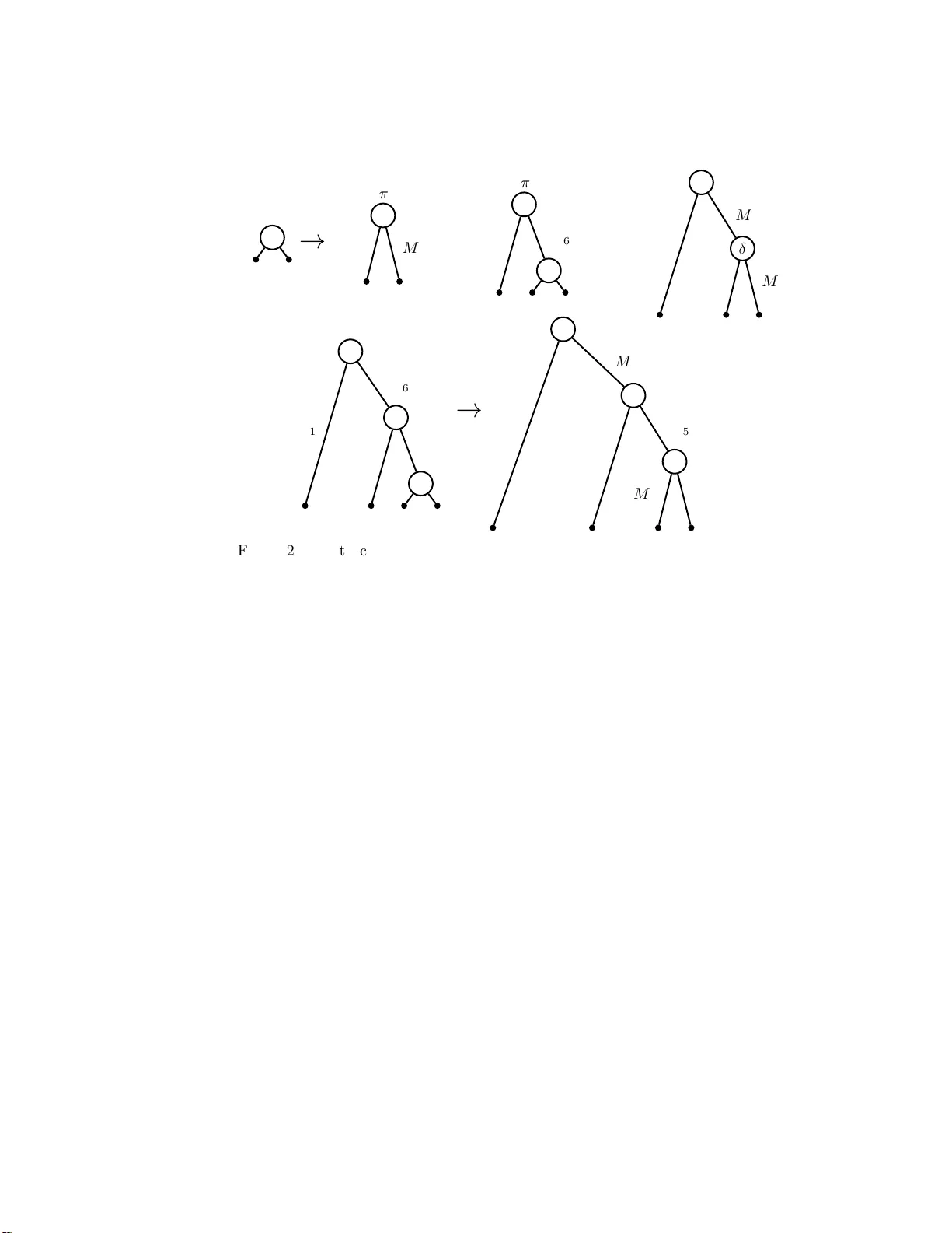
Mark o v in v arian ts, pleth ysms, and phyl ogenetics ∗ J G Sumner 1 , 2 , M A Charlesto n 1 , 4 , 5 , L S Jermiin 3 , 4 , 5 , and P D J arvis 2 , † 1 Scho ol of Information T e chnolo gies, 3 Scho ol of Biolo gic al Scienc es, 4 Centr e fo r Mathematic al Biolo gy, 5 Sydney Bi oinformatics, University of Sydney, N S W 2006, Austr alia 2 Scho ol of Mathematics and Physics, University of T asmania , T AS 7001, Austr alia Abstract W e explore mo del-ba s ed techniques of phylogenetic tree inference exer cising Ma rko v inv a riants. Marko v in v ariants a r e group inv a riant p olynomia ls and are distinct from what is known in the literature as phylogenetic inv a riants, although w e establish a commonality in so me s pe c ia l c a ses. W e show that the simplest Markov in v ariant forms the foundation of the Log -Det distance measur e . W e take as our primar y to ol gr oup r epresentation theory , and show that it provides a genera l framework for a nalyzing Marko v pro cesse s on trees . F ro m this algebr aic p ersp ective, the inherent symmetries of these pro cesses bec ome apparent, and fo cusing on plethysms, we are a ble to deﬁne Marko v in v ariants and give e xistence pro ofs. W e give an explicit technique for constr ucting the inv ariants, v alid for any num ber o f ch ar acter states and taxa. F or ph ylogenetic trees with three a nd four leaves, we demonstrate that the corr esp onding Marko v in v ariants can b e fr uitfully exploited in applied phylogenetic studies. ∗ This i s the “long v ersi on” that includes an extended introduction, a subsection on mi xed-w eight i nv ariants, a third appendix on the K3ST model, and a more rel axed pace with additional di scussion throughout . The “short version” appears in Journal of The or etic al Biolo g y , 253:601-615, 2008. † Alexander v on Humboldt F ello w keywor ds: inv arian ts, pleth ysm, phylogenet ics, Sc hur functions, branc hing rules email: js umner@it.usyd.edu.au UT AS-P H YS-2007-31 Con ten ts 1 In tro duction 1 1.1 Background . . . . . . . . . . . . . . . . . . . . . . . . . . . . . . . . . . . . . . . . 1 1.2 Marko v inv aria nts . . . . . . . . . . . . . . . . . . . . . . . . . . . . . . . . . . . . 3 2 Measure theory , the Mark ov sem igroup, and phy lo g enetic tensors 4 2.1 Probability mea sures on ﬁnite sets . . . . . . . . . . . . . . . . . . . . . . . . . . . 4 2.2 Random v ariables, genera ting function, expecta tio n v alues and estimators . . . . . 5 2.3 The Markov semigroup . . . . . . . . . . . . . . . . . . . . . . . . . . . . . . . . . . 7 2.4 Phylogenetic tensors . . . . . . . . . . . . . . . . . . . . . . . . . . . . . . . . . . . 9 2.5 Marko v inv aria nts, de ﬁnitio n . . . . . . . . . . . . . . . . . . . . . . . . . . . . . . 12 3 Group representation theory in phy log enetics 13 3.1 The Markov semigroup and aﬃliated g roups . . . . . . . . . . . . . . . . . . . . . . 13 3.2 Representations of GL ( k ) and Sc hur-W eyl dualit y . . . . . . . . . . . . . . . . . . . 14 3.3 Representations of × m GL ( k ) . . . . . . . . . . . . . . . . . . . . . . . . . . . . . . 17 3.4 Symmetric plethysms and inv ariants . . . . . . . . . . . . . . . . . . . . . . . . . . 18 3.5 Marko v inv aria nts, e xistence theorems . . . . . . . . . . . . . . . . . . . . . . . . . 19 4 Mark o v in v arian ts i n phylogenetics 21 4.1 Zo o of inv a riants and nomencla tur e . . . . . . . . . . . . . . . . . . . . . . . . . . . 2 1 4.2 What happ ens on a ph ylogenetic tree? . . . . . . . . . . . . . . . . . . . . . . . . . 2 2 4.3 Mixed weigh t Markov in v ariants . . . . . . . . . . . . . . . . . . . . . . . . . . . . 28 5 Discussion 29 A Pro of of Theorem 1 31 B The construction of Mark ov inv arian ts 33 C Kimura 3ST mo del and ph ylogeneti c in v arian ts 34 1 In tro duc tion 1.1 Bac kground Molecular phylogenetic metho ds aim to infer the pa s t evolutionary relationships o f organisms from present da y molecular data such as n ucleotide sequences. Pr o gress is made b y mak ing as tute assumptions ab out the e volutionary pro cess, whic h simplify the pro blem into a mathematical for m, while retaining muc h of the structure motiv ating the biological question at hand. This pro c e ss of mathematical mo de ling is esse nt ial if informed inference s from observed data sets ar e to be made. The most signiﬁcant simpliﬁcation made in phylogenetic mo dels is that the evolutionary change of the molecular units is assumed to progress by mutation under environmen tal inﬂuences and the Darwinian eﬀects of se lection are ignored. Another ov erriding simpliﬁcatio n, featuring in all the po pular models , is that the eﬀect o f mutations is mo delled as a sto chastic (rando m) pro c e s s assumed to b e Mar ko v. Also, it is often assumed that any given site in a molecula r seq uence evolv ed independently of the o ther sites, and the pr obability o f m utation a t each site is iden tically distributed (known together a s the I ID assumption). Although the IID a ssumption is kno wn not to hold in ma ny cases [58], we will assume throughout that I ID holds, and defer mo diﬁcation of the results presented here to this more genera l case. Much pr ogres s in ph ylogenetic inference has b een ac hieved in recent years with the use of so- phisticated mathematics, proba bility and statistical theory , a nd the adv ent o f pow erful computing techn iques . A general rule that rates the scientiﬁc credence of a ph ylog e netic metho d is that mo del b ase d techniques are preferred. In pa r ticular, some rece nt work has focus e d on the elucidation of 1 the implicit mo del a ssumptions o f p opular metho ds such as Neigh b or -Joining [9, 2 6] a nd Maxi- m um P ar simony [85]. This t yp e o f analys is is an essential part of the scien tiﬁc justiﬁcation because otherwise it is not exactly clea r what is being estimated in the statistical sense. Without such a framework the bio logist is left without any infor ma tion reg a rding the conﬁdence in the inference pro duced. An ov erlying diﬃculty in phylogenetic tree inference is that the num ber of po ssible tre es is v ast, and the spa ce of trees is non-Euclidea n; hence it is not clear ho w one should pro ceed in s e arching through it. It is norma l to begin with a candidate tree a nd then consider each of its neigh b ouring trees (under a given adjacency rule) and cho ose the new tree as that with the b est sco re. There is a range of a v ailable tree perturbatio n types suc h as “prune and regraft” or Nearest Neighbour Int erchange, which deﬁne these a djacencies. Which t yp e is preferable is a matter of o ngoing debate [14, 3 4] a nd such heuristic tec hniques sometimes ﬁnd only lo cally o ptimal so lutio ns. In this pap er we will not discuss the problems asso cia ted with la rge trees, but co nsider how small tree s may be built under ge neral mo del assumptions. W e give a ge neral framework for co nstructing small trees, whic h can then b e used as a springb oa rd for building large r trees using techniques suc h as ‘quartet puzzling’ [7 8] or sup er tr ee metho ds (for arbitr arily sized subtrees) [8, 89]. Due to its importanc e for calculating divergence times o f lineages, the rate of m utation present in mo dels of evolution is of central imp ortance in phylogenetics. There are several well-kno wn limitations of the s ta ndard mo dels inv olv ing the rate of mutation o n a phylogenetic tr ee. F o r instance, the I ID assumption is almost a lwa ys viola ted b y the exis tence of site-to- site rate v ariation [67] and by the existence o f inv ar iable sites [56]. Other issues include non-statio nary pro cesses of evolution (whic h leads to ‘co mpo sitional heterog eneity’ [44]), ‘pattern heter ogeneity’ (where the pattern of substitutions v a ries acr oss the sites [67]) and ‘heter otach y’ (diﬀerential rates across the tree) [57]. Ignoring the in v alidit y o f the simple mo dels when suc h as sumptions are v io lated leads to mo del mis-sp eciﬁcatio n [75] and (po tent ially ) incorrect tree inference. An issue for an y inference tec hnique is that of ‘consistency’; where consistency is always with resp ect to an ex plicit o r implicit mo del (or family of mo dels) of sequence evolution. Sta tis tica l consistency req uires that if the data set is sampled from a distribution genera ted under the mo del assumptions, then the inference metho d tends to the correct answer 100% of the time as the size of the data set (length of the sequences ) tends to inﬁnit y . F o r example F els enstein [21] showed that Maximum Parsimo ny (MP) is s ta tistically inc onsistent (with all but a small family of mo dels [74]). As exe mpliﬁed by the ﬁrs t three c hapters of the recent review b o o k [2 5], the statistically consistent, mo del ba sed ph ylogenetic methods can be placed in to three ca tegories: Minim um Evolution (ME) and distance based metho ds, Maximum Likelihoo d (ML), and Bayesian metho ds. ME pro ceeds by deﬁning a (mo del based) ma tr ix of pairwise distances b etw een the molecula r sequences, and then minimizes the total tree length acros s the space of possible trees sub ject to some sta tistical cr iteria s uch as least squares (see Chapter 1 of [25]). ML pro ceeds by maximizing the ‘likelihoo d’ of the o bserved da ta set a c ross the set of p ossible tre es and mo dels of evolution [22, 25]. B ay esian metho ds pr o ceed using Bayes’ theorem to ca lc ula te a pos terior distribution on the space of po ssible trees given a prior distribution (usually uniform–which is an issue in itself as this does not co rresp ond to any evolutionary model of tre e g eneration [9 3]). F or each o f these metho ds the underlying model assumptions are ex plicit, a nd curr ent research e ﬀo r ts revolve around implementing these metho ds under expanded ass umptions and/or in a computationally eﬃcient ma nner. Another desirable feature of any ph ylogenetic method is that the model o n whic h it is based should b e deﬁned by as few numerical parameters as p os sible. The iss ue of scientiﬁc conten t of a mo del a nd parameter coun ts is discussed b y Steel [75] in relation to the eﬀectiveness o f MP vs ML, where it was s ta ted that the “predictive pow er of the theory. . . tends to be dr owned out in a sea of parameter estimation”. This is a fundamen tal problem in mo del selection for biolog ical inference, and co rresp onds to what is known as the bias/v aria nce trade o ﬀ o f parameter estimatio n [11]; which in turn equates to the problem of “o verﬁtting” or “underﬁtting” a data set. F rom an information theoretic p er s pe ctive, a given data set contains only so muc h information from which the numerical para meters of a model ma y b e estimated. A model with many parameters may ﬁt 2 the data very well, in that the pa rameter es timates may b e close to their true v alues, but the corres p o nding v aria nces will be large be cause there are relatively few data po ints. On the other hand, the v ariance of the estimates of a mo de l with very few parameters will be smaller as there are man y data po int s to estimate each pa rameter, but in this case the model runs the risk of being badly mis-sp eciﬁed, so that the parameter estimates may b e biased. In this light, the ‘cov ario n’ mo del [69] deals with the eﬀects o f in v ariable sites whilst int ro ducing only one extra par ameter, and the ‘gamma ’ mo del [92] a ccounts for site-to-site rate v aria tio n, with only an additional tw o parameters . Other methods for coping with heterotach y , r ate v ariatio n and pattern hetero geneity include the partitioning of data s e ts and mixture models [67]. How ever, all of these metho ds suﬀer bec ause, in the genera l case, the mo dels must include an individual rate matrix (containing up to tw elve parameter s) and an edge length parameter for eac h and ev ery edge of the ph ylog e netic tree. In [70] it w as rec ent ly no ted that the task of ph ylogenetic tree inference often lies in a region where there are mor e pa rameters than data p oints. T o reduce the num b er o f para meters in phylogenetic mo dels, the evolutionary pro cess is usually assumed to b e stationar y and r eversible, the ra te matrices a re assumed to have a certa in for m (such as the J ukes-Can tor mo del with one para meter, or the Kim ura mo dels with tw o or three parameters ), and eac h edge of the ph ylogenetic tr ee is assigned the same r a te matrix (for details on these a ssumptions, see [10, 45]). T o a ccommo date non- s tationary pro cesses and asso ciated comp ositional heterog eneity , it b eco mes necessary to introduce many more par ameters in to the mo del. In this circumstance it then b eco mes desir able to use a tec hnique based on a gener al mo del but without the need to estimate the numerical parameters. In this ligh t, a matrix of Log- Det pairwise distances combined with the Neighbor-J oining algo rithm [59] achieves statistically consistent tree inference under the assumption of a genera l mo del. How ever this technique has its own shortcomings a s distance methods only conside r pairwis e sequence alignments, ignoring m uch of the information a v ailable in the data set, and has problems with model mis- sp eciﬁcation [84], and the statistical prope r ties of the Log -Det are not exa ctly kno wn [29]. A recently presen ted metho d [42] ﬁts a v ery general model, but clearly will hav e iss ues with ov er- pa rameteriza tion and computational requir ements. In summary , the desirable fea tures o f a given ph ylogenetic metho d are that it is based on a general model of se q uence e volution, it is statistically consistent with a family of known mo dels, and the num ber of parameters to b e estimated is minimal. 1.2 Mark o v in v arian ts In this work w e in tro duce the us e of ma thematical r epresentation theory to the pro blem of ph ylo- genetic inference (further background to the results is pres ented in the PhD thesis [81]). W e deﬁne ‘Marko v inv aria nts’ a nd show that these functions, when ev a luated on sequence data, can b e put to work in the problem of ph ylo g enetic tree inference under ra ther general mo del assumptions. Marko v inv a riants are distinct from what is k nown in the literatur e as ‘phylogenetic in v ariants’ [13, 19, 51, 77]. Marko v in v ariants are a pa rticular cas e of group in v ariant functions [6 6] and a re hence more constrained by deﬁnition than ph ylog enetic inv ariants. Some Marko v inv ariants are simult aneo usly phylogenetic inv aria nts, but the r everse is not true in genera l. The structure of Marko v in v ariants is more akin to that of the L o g-Det function [52, 59], whic h is constructed using the simplest exa mple of a Markov in v ariant, yet it is not a phylogenetic in v ariant. The app eal of this approach is that Mar ko v inv aria nts do not assume any particula r rate matrices or edge length parameter s on the phylogenetic tree. Broad conditions of molecular evolution a re thus accommo dated, incorp ora ting arbitrar y substitution rates, non-statio nary and time-inhomogeneous pro ce s ses, heterota chy , and arbitrar y pattern heter ogeneity a cross the tree. F urther, Marko v in v ariants sa tisfy certain alg e br aic r elations for particula r phylogenetic trees, and can provide a no vel metho d o f tree inference. This appro ach to ph ylog enetic tree inference sa tisﬁes the desirable features given in the sum- mary ab ov e. That is, Mar ko v inv ar iants are v alid for a g eneral mo del o f sequence evolution, statistical consistency is as sured, and only a few parameters need to be estimated. 3 In pa rticular, for the q ua rtet case, we give a tree inference ro utine, v alid for these inclusive conditions, optimizing o ver o nly one parameter. It is hoped that, with additio na l understanding , this technique can b e extended to large r tre e s. This will res ult in phylogenetic tree inference metho ds, v a lid for general models, that ma ke use o f o nly a few para meters. Suc h a p ossibility is very attractive, a s a ll of the data is utilized, a nd a gener al model may b e ass umed with the risk of ov erﬁtting signiﬁcantly re duce d. In this pap er we o utline the theo r etical background require d to understand the deriv ation of Markov inv arian ts. This will necess ita te, in § 2, an excur sion into elementary measure theory on ﬁnite sets, a nd the c o nstruction of ‘ph ylo genetic tensors ’. In § 3 we analyse ce r tain gro ups aﬃliated with the Marko v pro ces s, and review standard re s ults from group representation theory . This section concludes with a der iv ation of existence conditions for Mar ko v inv a riants. In § 4 we rep ort on the structure of Markov inv ariant s for phylogenetic trees with three and four lea ves, and give ex amples of how they can be incor p orated in to practical ph ylogenetic ana ly ses. 2 Measure theory , the Mark o v semigroup, and phylo genetic tensors In § 2.1 we co llect so me bas ic pro p e r ties of measur es on ﬁnite sets, justifying the use o f tensor pro duct spaces in the con text of Marko v pro cesses on ph ylog enetic tr ees. The res ults are r ather elementary , but ultimately neces sary to place the subse quent discuss ion on its prop er fo oting . See, for example, [30] for an in tro duction to measure theory . In § 2.2 we use gener ating function techn iques to c a lculate ex pe ctation v alues of v arious r andom v aria bles (and functions thereo f ) asso ciated with ph ylog e netic data sets. W e give a simple example and show how to compute its un bias e d estimator. W e deﬁne the ‘Ma rko v semig roup’ for the general time-inhomo geneous pr o cess ( § 2.3), construct ‘phylogenetic tensors’ ( § 2.4), and, ﬁnally , deﬁne Marko v inv ariants ( § 2.5). 2.1 Probabilit y measures on ﬁnite set s Consider a ﬁnite set lab elled b y natura l n umbers, K = { 1 , 2 , . . . , k } . A pr ob ability me asur e on K , is a function µ : K → [0 , 1 ], s uch that, for any pro p er subset A ⊂ K a nd any sequence A 1 , A 2 , . . . of pairwise disjoint subsets, the following conditions hold: µ ( ∅ ) = 0 , µ ( A ) < 1 , µ [ i A i ! = X i µ ( A i ) , µ ( K ) = 1 . W e denote the s e t o f pr o bability measures on K a s M ( K ). It follows from the third c ondition that for 1 ≤ i ≤ k the measur es, δ i ( A ) = 1 if i ∈ A and 0 otherwise, form a basis such that µ = k X i =1 µ i δ i , for all µ ∈ M ( K ) with µ i := µ ( { i } ). This deﬁnition is equiv alent to the usual r equirement of a probability distribution on a ﬁnite set: k X i =1 µ i = µ k [ i =1 { i } ! = µ ( K ) = 1 . In ph ylog enetics the data se ts under consideration a re a ligned sequences of mole c ula r units. F or example, in the ca s e of DNA made up of the four nucleotides adenine, cytosine, gua nine, thymine, 4 we would hav e K = { A, C, G, T } , k = 4 and write K = { 1 , 2 , 3 , 4 } . How ever, the results presented here and in § 3 a r e v alid for any k . In § 4 we will concentrate on ca ses relev an t to ph ylog enetics and in vestigate the Markov in v ariants for k = 2 , 3 a nd 4. In this work we do no t consider the pro blem of aligning the s equence data, a nd assume through- out tha t the ‘true’ alignment (without gaps) can a nd ha s b een fo und (where truth is relativ e to the mo delling pro cess). Under this circumstance, it b eco mes necessary to consider the direct product of K with itself m times: K m := × m K = K × K × . . . × K with | K m | = k m . Exactly as above, for any prop er subset E ⊂ K m and a ny sequence of pairwise disjoint s ubsets E 1 , E 2 , . . . , a probabilit y measure, µ ∈ M ( K m ), must equiv a le nt ly satisfy µ ( ∅ ) = 0 , µ ( E ) < 1 , µ [ i E i ! = X i µ ( E i ) , µ ( K m ) = 1 . Given that under a measure unions decompose in to summations, it follows that w e ha ve the tensor pro duct: M ( K m ) = ⊗ m M ( K ) := M ( K ) ⊗ M ( K ) ⊗ . . . ⊗ M ( K ) . Concretely , any subset of K m can be expressed as a union of disjoint subsets of the form A 1 × A 2 × . . . × A m , with A 1 , A 2 , . . . , A m ⊆ K . A ba sis for ⊗ m M ( K ) is then, for 1 ≤ i 1 , i 2 , . . . , i m ≤ k , δ i 1 ⊗ δ i 2 ⊗ . . . ⊗ δ i m ( A 1 × A 2 × . . . × A m ) := δ i 1 ( A 1 ) δ i 2 ( A 2 ) . . . δ i m ( A m ) , with δ i 1 ( A 1 ) δ i 2 ( A 2 ) . . . δ i m ( A m ) = 1 if { i 1 } ×{ i 2 } × . . . × { i m } ∈ A 1 × A 2 × . . . × A m and 0 otherwise. W e index the e lement s { i 1 } × { i 2 } × . . . × { i m } as I = i 1 i 2 . . . i m , and write µ I ≡ µ i 1 i 2 ...i m := µ ( { i 1 } × { i 2 } × . . . × { i m } ) . W e refer to m a s the r ank of the tensor µ . Previous ly the author s JGS and PDJ have presen ted pro ba bility distributions on ph ylogenetic trees in a tensor pro duct fo r malism motiv ated from ana logies to qua ntum ph ysics [40, 8 3]. The formulation prese nted a bove places this constr uction on its pr op er measure-theor etic fo oting 1 . In § 2.4 w e will re la te a given (Markov) model of evolution on a phylogenetic tree with m leav es, to a unique rank m tensor P ∈ ⊗ m M ( K ). 2.2 Random v ariables, generating function, exp ectation v alues and es- timators An y da ta set consider ed in a phylogenetic study is necessar ily of ﬁnite extent, and we supp os e that it is a sample drawn from some unknown distribution. W e wish to deﬁne exp ecta tion v alues of such data (or event s) and functions thereof. Througho ut w e will assume the IID assumption 1 W e are indebted to Michae l Baake for dra wing our atte ntion to this. 5 holds, so that w e need only consider the distribution of a single random v ariable. The probability of obser v ing a particular state at a given site will be iden tical for all the o ther sites. F or a set of m aligned s e quences o f length N , deﬁne a p attern to b e the (ordered) set of s tates read a cross the m sequences at a pa rticular site in the alignment. Tha t is , a pattern takes the form I = i 1 i 2 . . . i m , where i a is the character s tate in the a th sequence. Deﬁne the ra ndom v aria ble X as the pattern obser ved at a given site. A probability distribution for X c an be sp eciﬁed using a probability measure µ ∈ ⊗ m M ( K ): P [ X = i 1 i 2 . . . i m ] = µ i 1 i 2 ...i m . (1) F or a sequence of ﬁnite length N , deﬁne Z as the r a ndom v ariable that co un ts the num b er of o ccurrences of ea ch pattern I = i 1 i 2 . . . i m in the alignment, so that Z = ( Z I ) = ( Z i 1 i 2 ...i m ) 1 ≤ i 1 ,i 2 ,...,i m ≤ k , and P I ∈ K m Z I = N . A ssuming that each site in the a lig nment is ident ica lly and independently distributed as (1), it follo ws that Z is multinomially distributed under the measur e µ : P [ Z = z ; N ] = Y I ∈ K m N ! z I ! µ z I I . This ex presses, under the a ssumptions o f µ , the pr obability of obser ving within the a lignment of m sequences the sp eciﬁc num b er of o ccurrences of each o f the p ossible character patterns Z = z . When w e describ e Mar ko v inv a riants, w e will need to discuss expecta tion v alues of the random v ariable Z and functions thereof. F or an y function φ , the e xp ectation v alue with resp ect to the measure µ is deﬁned a s E [ φ ( Z )] := X z φ ( z ) P [ Z = z ; N ] , with the summation ov er all z s uch that P I ∈ K m z I = N . Remem b ering that Z follows a mu ltinomial distribution, it is in practice nece ssary to use generating function tech niques in o rder to calculate thes e ex p ec ta tion v alues. The genera ting function on the for mal v ariables s = ( s I ) = ( s i 1 i 2 ...i m ) 1 ≤ i 1 ,i 2 ,...,i m ≤ k of the multinomial distribution is G ( s ) := E [ e ( s,Z ) ] = X I ∈ K m µ I e s I ! N , (2) with ( s, Z ) := X I ∈ K m s I Z I . F rom the prop er ties of the exp onential function and the commutivit y of diﬀerentiation a nd exp e c- tation, ∂ G ( s ) ∂ s i 1 i 2 ...i m     s =0 = E [ Z i 1 i 2 ...i m ] . Using the ab ov e closed form of the g enerating function, an elementary calculation returns E [ Z i 1 i 2 ...i m ] = N µ i 1 i 2 ...i m , as of course w ould be expected. This ca n b e extended to ﬁnd the exp ectation of an y function of Z : E [ φ ( Z )] = φ  ∂ ∂ s  G ( s )     s =0 . 6 As a c o ncrete exa mple, take m = 2 a nd consider the case φ ( Z ) = Z 2 44 − Z 12 Z 13 . F rom the linearity of the expectation v alues we ha ve E [ Z 2 44 − Z 12 Z 13 ] = E [ Z 2 44 ] − E [ Z 12 Z 13 ] , so we ca n consider each term in tur n. T aking deriv atives of the closed form of the gener ating function gives E [ Z 2 44 ] = N ( N − 1) µ 2 44 + N µ 44 and E [ Z 12 Z 13 ] = N ( N − 1) µ 12 µ 13 . Thu s, in this case, the exp ectation v alue of φ is E [ φ ( Z )] = N ( N − 1 )( µ 2 44 − µ 12 µ 13 ) + N µ 44 . Given a (po ssibly unobserv able) r andom v ariable θ , a n estimator is another random v ar iable which is a function of observ able quan tities suc h that its expecta tion v a lue somehow approximates θ . The bias o f an estimator b θ is deﬁned as the diﬀerence b ( ˆ θ ) = E [ b θ ] − E [ θ ] , allowing for θ to simply b e a co nstant so that E [ θ ] = θ . An unbiase d estimator is simply an estimator with bias equal to zero. F or ex ample, a short calculation reveals that the unbiased estimator of φ ( µ ) ab ove is φ ( Z ) − Z 44 N ( N − 1) . In g eneral, if φ is p olynomial, computing an unbiased form is a str aightforw ar d matter of solving a seq ue nce of diﬀere nce equations. When it comes to discussing estimator s for Marko v inv ariants, we w ill show tha t unbiased for ms can easily b e deﬁned. Howev er, we will no te that explicit computation is diﬃcult due to a required change o f basis. 2.3 The Marko v semigroup A sto chastic proc e ss can b e describ ed b y in tro ducing a time-dep endent random v ariable X ( t ). A crucial comp onent of the subseq uent discussion will b e that the time evolution o f the corr esp onding probability distribution ca n b e view ed a s a linear mapping upon a vector space. Presently we will establish the conditions for a Markov pr o cess, and show that such a proces s satisﬁes the des ired prop erty . See , for example, [38] for an eq uiv alen t deriv ation. Consider a time-dependent, ﬁnite-state rando m v ariable, X ( t ), taking on v a lues in K , any set of times t 1 < t 2 < . . . < t n < t , and the joint distribution of X acros s those times: P [ X ( t 1 ) = i 1 , X ( t 2 ) = i 2 , . . . , X ( t n ) = i n , X ( t ) = i ] . The distribution of X at the particular time t is giv en by the marginal, P [ X ( t ) = i ] = X 1 ≤ i 1 ,i 2 ,...,i n ≤ k P [ X ( t 1 ) = i 1 , X ( t 2 ) = i 2 , . . . , X ( t n ) = i n , X ( t ) = i ] , and this can b e re-expressed b y inv oking the conditional distribution: P [ X ( t ) = i ] = X 1 ≤ i 1 ,i 2 ,...,i n ≤ k P [ X ( t ) = i | X ( t 1 ) = i 1 , X ( t 2 ) = i 2 , . . . , X ( t n ) = i n ] · P [ X ( t 1 ) = i 1 , X ( t 2 ) = i 2 , . . . , X ( t n ) = i ] . 7 The simplest sto chastic pr o cess is the pro cess for which the pr obability o f a transition to a new state at a given time is indep endent of the states a t all pr eceding times (suc h as tossing of a coin–the Bernoul li pr o c ess ). A Markov pr o c ess ca n be seen a s the next simplest case where the probability of a tra nsition is indep endent o f a ll but the state at the mos t r ecent time. Thus, for a Marko v pro c ess the conditional distributio n sa tisﬁes P [ X ( t ) = i | X ( t 1 ) = i 1 , X ( t 2 ) = i 2 , . . . , X ( t n ) = i n ] = P [ X ( t ) = i | X ( t n ) = i n ] . This implies that the mar ginal distribution of X at the time t is P [ X ( t ) = i ] = X 1 ≤ i n ≤ k P [ X ( t ) = i | X ( t n ) = i n ] · X 1 ≤ i 1 ,...,i n − 1 ≤ k P [ X ( t 1 ) = i 1 , X ( t 2 ) = i 2 , . . . , X ( t n ) = i n ] = X 1 ≤ i n ≤ k P [ X ( t ) = i | X ( t n ) = i n ] P [ X ( t n ) = i n ] . Int ro ducing the time-dep endent measur e µ t with µ t ( { i } ) := µ t i = P [ X ( t ) = i ], we can express this as µ t i = X 1 ≤ j ≤ k M ij ( t, s ) µ s j , for all s < t , and for M ij ( t, s ) := P [ X ( t ) = i | X ( s ) = j ]. If we consider the ( M ij ( t, s )) 1 ≤ i,j ≤ k as the matrix elements of a linear op era tor M ( t, s ) acting on the vector space R k ⊃ M ( K ) with basis elements δ 1 , δ 2 , . . . , δ k , we see that, as pro mis e d, for a Markov pro cess the time evolution of the probability distribution is given b y a linea r map on R k deﬁned by its action on time-dep endent probability measures: µ s M ( t,s ) 7→ µ t , µ t = M ( t, s ) µ s . (3) This linear map descr ib e s the genera l time-inhomogeneous ﬁnite state Ma r ko v pr o cess and can easily b e extended to the whole of R k . In [83] JGS a nd PDJ co nsidered sto chastic matrices as elements of the genera l linear group, and used this prop erty to study the structure of inv a riant p olyno mials (used as measures of ent ang lement in quantum physics) when ev aluated o n a phylogenetic tree. Presently we will deﬁne the Mar ko v semigroup which serves to reﬁne the deﬁnition of inv ar ia nt functions to the more relev ant cas e of a sto chastic (but linea r) time evolution. Deﬁne the time-dep endent r ate matrix , Q ( t ), as a (contin uous) one-para meter family of lin- ear op er ators o n the vector space M ( K ), which in the δ 1 , δ 2 , . . . , δ k basis has matrix elements satisfying: Q ij ( t ) ≥ 0 , ∀ i 6 = j ; Q ii ( t ) = − X j 6 = i Q j i ( t ) . The summation conditions can b e equiv alently expre ssed by deﬁning the vector θ = δ 1 + δ 2 + . . . + δ k and its transp os e θ ⊤ , and setting θ ⊤ Q ( t ) = 0 , for all t . The Marko v semigro up on k elements, M ( k ), with parameters 0 ≤ s ≤ t < ∞ , is deﬁned as the subset of (diﬀerentiable) t wo-parameter linear op erator s o n M ( K ) which satisfy M ( t, s ) = 1 , ∀ t = s ; 8 the Chapman-Ko lmogor ov equation: M ( t, s ) M ( s, r ) = M ( t, r ) , ∀ r < s ; and the backw ards and forwards equations: ∂ M ( t, s ) ∂ s = − M ( t, s ) Q ( s ) , ∂ M ( t, s ) ∂ t = Q ( t ) M ( t, s ); (4) for a ny ra te matrix Q ( t ) [27, 38]. Solutions o f (4 ) c a n b e repre s ented using the time-ordered pro duct (or or dered-exp one ntial): M ( t, s ) = T exp Z t s Q ( u ) du (5) [39, Chap. 4], from which it follows tha t det M ( t, s ) = exp Z t s tr ( Q ( u )) du, (6) and θ ⊤ M ( t, s ) = θ ⊤ . The time-order ed product is b est understoo d by considering the appr oximation M ( s + 2 ǫ, s ) = M ( s + 2 ǫ, s + ǫ ) M ( s + ǫ, s ) ≃ e Q ( s + ǫ ) ǫ e Q ( s ) ǫ . By co nsidering (4) for the case t = s , it follows that in the δ 1 , δ 2 , . . . , δ k basis, the ma trix elements of each M ( t, s ) lie in the interv al [0 , 1] for all s ≤ t . Thu s, the Markov s emigroup corres p o nds to the subset of the set of sto chastic matrices sub ject to the condition that for eac h matrix ther e exists a rate matrix (or gener ator) Q ( t ) suc h that (5) is satisﬁed. W e refer to elemen ts of the Mar ko v semig roup as Markov op er ators . In the time-homogeneous case wher e the rate matrix is time-independent: Q := Q ( t ) = Q (0) , it follows that M ( t, s ) is dependent only up on the diﬀerence ( t − s ), and for m (5) becomes simply M ( t ) = e tQ = X 0 ≤ n< ∞ ( tQ ) n n ! . In § 3 w e will discuss some representation-theoretic pro pe rties o f certain groups a ﬃlia ted with the Marko v semigroup. 2.4 Ph ylogenetic tensors A tree, T , is a connected g raph without c y cles and consis ts of a set of vertices and edges. V ertices of degree o ne are calle d le aves . W e work with oriente d tree s, which are deﬁned by directing each edge of T aw ay from a distinguished v ertex , ρ , known as the r o ot o f the tr e e. Conse quently , a given edge lying b etw een a djacent v ertices u and v is spe ciﬁed as an ordered pa ir ( u, v ), where u lies on the unique path fro m ρ to v . A cherry is a pair of leaf v ertices with the same pa r ent vertex. Assign a r andom v aria ble, X v , to ea ch vertex of the tree, and, as descr ib ed in [7 2, Chap. 8 ], a joint distr ibution of the random v ariables at the leav es is determined b y specifying a distribution π ∈ M ( K ) at ρ and a Marko v opera tor M v, u ∈ M ( k ) for ev ery edge ( u, v ). In particular , for every 9 π δ b M 1 b M 2 Figure 1: Phylogenetic tree with tw o leaves v , the random v aria ble X v is co nditional on o nly the random v ariables lying on the path fro m ρ and v , and for each pair of vertices v 1 , v 2 with common par ent u , the jo int distr ibutio n of X v 1 and X v 2 is given by P [ X v 1 = i 1 , X v 2 = i 2 ] = X 1 ≤ j ≤ k M v 1 ,u i 1 j M v 2 ,u i 2 j µ u j , (7) where µ u is the distribution of X u . The empirica l int er pr etation of the joint distribution across the leaves is that of a s ampling distr ibution fr om which an alignment of molecular s equences is constructed b y drawing one character pa tter n at a time. Througho ut this paper, we will cons ider ph ylo genetic trees where the ro ot distribution and the Mar ko v o p erators are arbitra ry . Note that we insist that the Mar ko v op erator s b elo ng to the Markov semig r oup, s o a co nt inuous- time pro cess is in action throughout the tree. This additional ana lytic structure means that this mo del is slightly less general than the gener al Markov mo del a s deﬁned in [1, 4 1]. The g eneral Marko v mo del allo ws for arbitrar y tra nsition matr ices with positive entries and unit row-sum (unit column-sum in o ur for m ulatio n), and it is not hard to ﬁnd a matrix satisfying these conditions but with determinant less than or equal to zer o, directly contradicting (6). W e will co nsider a jo int pr o bability distribution on m leav es as a probability measure, P ∈ ⊗ m M ( K ), that we refer to a s a phylo genetic tensor . Pr e sently we review how these tensors can be constructed using purely alg ebraic opera tions. The branching pro cess (7) ca n be interpreted as a map that takes probability mea sures on K to probability measures on K × K = K 2 . In [40, 83], it was shown how to formalize this by deﬁning the linear op era tor δ : M ( K ) → M ( K ) ⊗ M ( K ) . Demanding the conditional dep endencies that a re r equired for the standard deﬁnition of a tree distribution [72, Cha p. 8], we ha ve (expres sed in the δ 1 , δ 2 , . . . , δ k basis) the sp eciﬁcation δ : δ i 7→ δ i ⊗ δ i , 1 ≤ i ≤ k . The phylogenetic tr ee with tw o leav es (Figure 1) can then b e represented as the string P = ( M 1 ⊗ M 2 ) · ( δ · π ) , where M 1 and M 2 are the Mar ko v op erato rs on the t wo edges of the tree a nd, if X 1 and X 2 are the random v ariables at the leav es 1 and 2, re s pe ctively , we hav e P [ X 1 = i, X 2 = j ] = P ij := P ( { i } × { j } ) . This cons tr uction can b e genera liz ed to any ph ylo g enetic tree by colo uring the r o ot o f the tree with a distribution π , ea ch in ternal v ertex (including the root) with a br anching ope rator δ , a nd every edg e with an arbitra ry Markov op erator. The phylogenetic tensor is constructed by b eginning at the ro o t of the tree, and then recursively mo ving to the child vertices and applying the relev ant op erator s to the corre sp onding s lots in the (growing) tensor . Whenever a leaf is encountered, contin ually apply the identit y op erator at that leaf, until all leav es hav e b een reached and the ph ylo genetic tensor is complete. A phylogenetic tensor, P , is then r e presented as a str ing made 10 π • → π δ b b → π δ b M 1 b M 6 → π δ b M 1 δ M 6 b b → π δ b M 1 δ M 6 b M 2 b M 5 → π δ b M 1 δ M 6 b M 2 δ M 5 b b → π δ b M 1 δ M 6 b M 2 δ M 5 b M 3 b M 4 Figure 2: Constr ucting the phylogenetic tensor for a four taxon tree up of the c har acters π , M 1 , M 2 , . . . , and δ , and the joint distribution o f the r andom v ariables X 1 , X 2 , . . . , X m at the leav es 1 , 2 , . . . , m is given by P [ X 1 = i 1 , X 2 = i 2 , . . . , X m = i m ] = P i 1 i 2 ...i m := P ( { i 1 } × { i 2 } × . . . × { i m } ) . F or example, the phylogenetic tensor of four leaves (Figure 2) is re presented by the string P = (1 ⊗ 1 ⊗ M 3 ⊗ M 4 ) · (1 ⊗ 1 ⊗ δ ) · (1 ⊗ M 2 ⊗ M 5 ) · (1 ⊗ δ ) · ( M 1 ⊗ M 6 ) · ( δ · π ) , and is constructed in the steps π → δ · π → ( M 1 ⊗ M 6 ) · ( δ · π ) → (1 ⊗ δ ) · ( M 1 ⊗ M 6 ) · ( δ · π ) → (1 ⊗ M 2 ⊗ M 5 ) · (1 ⊗ δ ) · ( M 1 ⊗ M 6 ) · ( δ · π ) → (1 ⊗ 1 ⊗ δ ) · (1 ⊗ M 2 ⊗ M 5 ) · (1 ⊗ δ ) · ( M 1 ⊗ M 6 ) · ( δ · π ) → (1 ⊗ 1 ⊗ M 3 ⊗ M 4 ) · (1 ⊗ 1 ⊗ δ ) · (1 ⊗ M 2 ⊗ M 5 ) · (1 ⊗ δ ) · ( M 1 ⊗ M 6 ) · ( δ · π ) . In order to deﬁne Marko v inv a riants, we must a lso de ﬁne t wo reduced tens o rs based on P , the trimme d tenso r e P a nd the prune d tensor P ∗ . These are both constructed by mo difying the underlying tree. The trimmed tensor e P is co ns tructed by taking P and setting the Markov op erator s on the penda nt edges all equal to the iden tity op erator , or equiv alen tly s etting the lengths of the p endant edg es to zero . The pruned tensor P ∗ is co nstructed b y removing all cherries from the trimmed tensor. The rank of the pruned tensor is ( m − c ) wher e c is the n umber of cherries on the underlying tree. In the general case, we can relate P and e P as P = ( M 1 ⊗ M 2 ⊗ . . . ⊗ M m ) · e P , (8) where M 1 , M 2 , . . . , M m are the Marko v o p erators on the leaf edges. In what is to come, we will contin ually use this relatio n. As an illustration o f the relationship b etw een P , e P a nd P ∗ , ta ke the sev en leaf tree (Figur e 3), with phylogenetic tensor given by P = (1 ⊗ M 2 ⊗ M 3 ⊗ M 4 ⊗ M 5 ⊗ M 6 ⊗ M 7 ) · (1 ⊗ δ ⊗ δ ⊗ δ ) · ( M 1 ⊗ M 8 ⊗ M 9 ⊗ M 10 ) · ( δ ⊗ δ ) · ( M 11 ⊗ M 12 ) · ( δ · π ) . 11 The trimmed tensor co r resp onding to the tree (Figure 4) is obtained by clipping oﬀ the pendant edges: e P = (1 ⊗ δ ⊗ δ ⊗ δ ) · (1 ⊗ M 8 ⊗ M 9 ⊗ M 10 ) · ( δ ⊗ δ ) · ( M 11 ⊗ M 12 ) · ( δ · π ) , and, ﬁnally the pruned tenso r corresp onding to the tree (Figure 5) is expressed as: P ∗ = ( M 8 ⊗ M 9 ⊗ M 10 ) · (1 ⊗ δ ) · ( M 11 ⊗ M 12 ) · ( δ · π ) . 2.5 Mark o v in v arian ts, deﬁnition With the form (8) in mind, we deﬁne a Marko v invariant of weight ( w 1 , w 2 , . . . , w m ) as a function satisfying f ( P ) = (det M 1 ) w 1 (det M 2 ) w 2 . . . (det M m ) w m f ( e P ) , (9) for all M 1 , M 2 , . . . , M m ∈ M ( k ). W e exclusively c o nsider po lynomial functions, and wher e w 1 = w 2 = . . . = w m ≡ w , the Mark ov inv ar iant is sa id to b e of weigh t w . Considering the ab ove dis cussion o f un biased e s timators o f ra ndom v ariables, an unbiased estimator of a Markov inv ar iant is a function, b f , such tha t E [ b f ( Z )] = f ( P ) = (det M 1 ) w 1 (det M 2 ) w 2 . . . (det M m ) w m f ( e P ) . Such an es timator depends, up to the multiplicativ e s caling factor, only up on the internal str ucture of the phylogenetic tree. It is exactly this property that can be pro ductively engaged in the co nt ext of phylogenetic tr ee inference. Conv ersely , a phylo genetic invariant is a function satisfying f ( P ) ≡ 0 for all P b elo nging to the family o f phylogenetic tenso r s a rising from a particular tree (or s ubset of tr e es). In § 4 w e will show that there exist Mark ov inv aria nts for trees with three a nd four lea ves that ar e simultaneously ph ylo genetic inv aria nt s. Given a Mar ko v in v ariant, f , co nsider the induced function, f ∗ , deﬁned o n pruned tensors and sp eciﬁed by e v aluating the trimmed tensor: f ∗ ( P ∗ ) = f ( e P ) . This induced function is easily extended to b e deﬁned up on all of ⊗ m − c M ( K ), wher e c is the nu mber of c herr ie s on the underlying tr e e of P . Such case s ar e of sp ecial interest for ph yloge ne tic problems. In § 4 we will review a case (repo r ted in a less general con text in [84]) where this induced function is itse lf a Markov inv ar ia nt. W e exp ect that future inv estigations of Markov inv aria nt s will reveal more cases suc h as this. In § 3.5 w e will establish existence conditions for Marko v in v ariants using standard results from group representation theo ry . π δ δ M 11 b M 1 δ M 8 b M 2 b M 3 δ M 12 δ M 9 b M 4 b M 5 δ M 10 b M 6 b M 7 Figure 3: Phylogenetic tensor P for s e ven taxo n tr ee ((1,23 ),(45 ,67)) 12 π δ δ M 11 b δ M 8 b b δ M 12 δ M 9 b b δ M 10 b b Figure 4: T rimmed ph ylogenetic tensor e P π δ δ M 11 b b M 8 δ M 12 b M 9 b M 10 Figure 5: Pr uned ph ylog enetic tensor P ∗ 3 Group represen tation theory in p h ylogenetics In this sectio n we use the algebraic description of probability distributions on ph ylogenetic trees given in § 2 .4 to esta blish natural connections with asp ec ts of repres ent atio n theo ry , for certa in groups aﬃliated to the Markov semigr oup. These are discussed in § 3.1. T he n follows ( § 3 .2 and § 3.3) a brief outline of those a sp ects of the repres entation theor y of the genera l linear group and its subg roups that ar e needed for the discussio n of gr oup branching r ules. This leads to the construction of one-dimensional repres ent atio ns and their identiﬁcation as inv a riants ( § 3.4), with existence conditions given in § 3.5. 3.1 The Marko v semigroup and aﬃliated groups The linear tra nsformation (3) eﬀected under the Mar ko v semigroup on pr o bability mea s ures is closely related to c e rtain g roup ac tio ns on the vector space R k . Giv en that the c orresp o nding representation theory is unc hanged [4 8], in this sec tio n we w ill g eneralize to complex vector space, (as with [1]). That is, here and below, for algebraic purp oses w e regar d the δ 1 , δ 2 , . . . , δ k as elements of a basis for V ∼ = C k . Thus, the probability measures b eco me a subset lying in the ambien t c o mplex space ⊗ m C k ⊃ ⊗ m M ( K ). F or related co nsiderations inv olving the study of inv ariants o f sto chastic matrices see [46, 65]. Referring to (6) and noting that −∞ < tr ( Q ( t )) ≤ 0 for all t , the determinant of ea ch elemen t M ( t, s ) lies in the in terv al (0 , 1], and the Ma rko v semigr oup o ccur s as a subset o f the general linear group: M ( k ) ⊂ GL ( k ) . GL ( k ) is the group o f invertible linear op er ators on the k -dimensional vector spa ce C k . The smallest subgroup of GL ( k ) that con tains M ( k ) is obtained b y taking M ( k ) toge ther with all of its op erator inv erse s . In order to apply known methods of representation theor y , we will, how ever, not work with this g r oup directly . W e deﬁne a slig ht ly less reﬁned subgro up as the focus o f the impending discussion. Generalizing the notation o f [65], w e deﬁne the s ubgroup GL 1 ( k ) ⊳ GL ( k ) as the subse t of GL ( k ) 13 whose matrices in the δ 1 , δ 2 , . . . , δ k basis hav e unit column-sum. That is, for all g ∈ GL 1 ( k ): θ ⊤ g = θ ⊤ . The gro up pr op erty clearly holds, as for all g 1 , g 2 ∈ GL 1 ( k ): θ ⊤ ( g 1 g 2 ) = ( θ ⊤ g 1 ) g 2 = θ ⊤ g 2 = θ ⊤ . This gro up is isomorphic to the complex aﬃne gr oup 2 GL ( k − 1) ⋉ T ( k − 1) ≡ A ( k − 1 ) , where T ( k − 1 ) is the group of linear translations on C k − 1 . As shown in App endix A, this isomorphism is due to the column-sum c ondition be ing, in eﬀect, a statement that the gro up elements a re dual to linear transforma tions in k -dimensional co mplex space, leaving a ﬁxed vector inv ariant. Consider also the doubly-sto chastic Marko v semigroup, M ∗ ( k ), obtained b y requiring an addi- tional condition on the r ate matrices: Q ( t ) θ = 0 . The asso ciated subg roup o f the general linear g r oup is then denoted as GL 1 , 1 ( k ); the subg roup o f matrices in GL ( k ) which hav e unit column- and row-sum with, for all g ∈ GL 1 , 1 ( k ): θ ⊤ g = θ ⊤ , g θ = θ. Again the gro up pr op erty can eas ily b e sho wn to hold. Thus the doubly-sto chastic Markov semi- group is naturally aﬃliated to the as so ciated group GL 1 , 1 ( k ) which, a lso as sho wn in Appendix A, itself is iso mo rphic to GL ( k − 1). T o summarise, consider the s ubg roup c hain: GL ( k − 1) ∼ = GL 1 , 1 ( k ) ⊳ GL ( k − 1) ⋉ T ( k − 1) ≡ A ( k ) ∼ = GL 1 ( k ) ⊳ GL ( k ) . (10) and the set inclusions : M ( k ) ⊂ GL 1 ( k ) , M ∗ ( k ) ⊂ GL 1 , 1 ( k ) . W e now hav e a clear picture of how to develop the r epresentation theo ry of the Markov semi- group whic h foc uses on alg ebraic prop erties and avoids the analytic details due to the positivity requirement a nd semigroup prop er t y . This is the cor rect framework in whic h to exploit the Sch ur- W eyl dualit y ( § 3.2) and, cons idering the ab ove inclusions, all r esults presented will b e v alid for the Marko v semigroup. The ab ove subgroup chain will fea ture in § 3.4 where we give existence conditions for Markov inv ar iants. 3.2 Represen tations of GL ( k ) and Sch ur-W eyl dualit y Our pur p o se here is to show that the close relation of the Markov semigroup to aﬃliated subgroups of the general linea r gr oup allows the machinery o f repres ent atio n theory to b e applied in analysing the mo dels used in phylogenetic inference. F rom the form of the gener al Mar ko v mo del on phylogenetic trees given ea rlier (8 ), it is evident that the repr esentation-theoretic considera tions m ust b e ex tended to tenso r pro ducts. W e now provide some sta nda rd results within this se tting (see, for example, [24, Lecture 6]). 2 The symbol ⋉ denotes the semi-dir e ct pr o duct of t wo gr oups [3, Chap. 1]. The standard ph ysical example is the Euclidean group, which o ccurs as the semi-dir ect pr oduct b et ween rota tions and translations in R n . These are none other than the s et of transformations th at deﬁne Euclidean geometry . 14 F or GL ( k ) and its classical subgro ups it is well known that for the deﬁning repr esentation on V ∼ = C k , with v 7→ g v , extended to a reducible representation on ⊗ m V in the o bvious wa y , v 1 ⊗ v 2 ⊗ . . . ⊗ v m 7→ g v 1 ⊗ g v 2 ⊗ . . . ⊗ g v m , there is a dir e ct sum decomp osition, ⊗ m V = X λ ⊢ m ⊕ f λ V λ , (11) int o (p ossibly reducible) subspaces V λ . These subspaces (or mo dules ) are lab elled by integer partitions, λ = ( λ 1 , λ 2 , . . . , λ n ), of m , the λ i being nonzero and nonincre a sing and s uch that λ 1 + λ 2 + . . . + λ n = m . If λ is a partition o f m , we write λ ⊢ m and | λ | = m . The c o rresp o nding mo dule V λ is determined b y a unique pro jector o n ⊗ m V ; the Y oung’s op er ator Y λ . The f λ are int eger m ultiplicities determining how many times each mo dule o c c urs in the decomp osition. The Schur-Weyl duality is the classic result that each f λ is none other than the dimensio n of the irreducible representation asso ciated with the same partition λ of the symmetric g roup S m . This reﬂects the role of the symmetric group’s action on ⊗ m V by per mut ing bas is ele ment s acr oss the tensor pro duct, when co ns tructing the Y oung’s op er ators. The char acter of a r epresentation is deﬁned as the set of traces of the repres e nt ing matrices; one for ea ch g roup element. The ir reducible r epresentations of a group can b e enumerated b y solely considering the corr esp onding irreducible c hara cters. Thus the problem of decompo sing a representation int o irreducible mo dules (computing the m ultiplicities f λ ) can be per fo rmed at the level of the c hara cters 3 . F or instance, in the case of GL ( k ) itself, the V λ are irreducible, with character given by the celebrated Sch ur functions, s λ , with s λ ( x ) = tr( π λ ( g )) , where π λ ( g ) is the representing matrix for gr oup element g and x 1 , x 2 , . . . , x k are its eige nv alues. The Sch ur functions are deﬁned in their own right, and are uniquely determined by the semi- standard tableaux co r resp onding to the partition λ [60]. The deﬁning k -dimensional repr esentation in this notatio n is V { 1 } ∼ = C k , in which case the Sch ur function is s { 1 } ( x ) = x 1 + x 2 + . . . + x k . The Sc hur functions form a basis for the ring of symmetric functions on any n umber of v ariable s , and the trace is a symmetric function. Hence, the pr oblem of iden tifying the ir r educible GL ( k ) mo dules in the ab ov e repr esentation o n ⊗ m V , reduces to identif ying the Sch ur functions in the decomp osition of the character with resp ect to this basis 4 . A c o nv enient a nd standard notation for Sch ur functions is given by enclosing the partition (or parts thereof ) in brace s [54]. Th us { λ } a nd { 1 } , are the Sch ur functions co rresp o nding to a general irreducible and the deﬁning representation of GL ( k ) res p ec tively . F or simplicity , w e write π { 1 } ( g ) = g . F or classical subgr oups of GL ( k ), the mo dules V λ are no longer necessar ily irreducible, and further combinatorial consider a tions (not required here) are nee de d to eﬀect a complete reduction 5 . More impor tantly , for GL ( k ) itself with V not the deﬁning, but an arbitrar y mo dule, V ρ say , the equiv alen ts of the abov e mo dules, ( V ρ ) λ , are again no long er irreducible in genera l. This construction introduce s a fundamen tal op eration for com bining representations together; that of plethysm [54]. The character of ( V ρ ) λ is denoted { ρ }⊗ { λ } ; the plethysm of { ρ } b y { λ } . In the simplest case { ρ } is the character for the deﬁning r epresentation, { 1 } , and by deﬁnitio n { 1 }⊗ { λ } = { λ } . In general, for a ny symmetric functions A, B we ha ve { ρ }⊗ ( A + B ) = { ρ }⊗ A + { ρ }⊗ B , a nd 3 Within the con text of ph ylogenetics, see [62] for an unrelated di scussion of the irreducible characte rs of the symmetric group. 4 The stronger statemen t that the V λ prov ide the complete s et of irreducible mo dules of any in tegral represen- tation of GL ( k ) is v alid [48]. 5 The classical subgroups of GL ( k ) are constructed by requiring, under the group action, the inv ariance of bilinear forms on V . 15 we recover { ρ }⊗  X λ ⊢ m f λ { λ }  = { ρ } ⊗ { ρ } ⊗ . . . ⊗ { ρ } , where { ρ } ⊗ { λ } denotes the (comm utative and asso ciative) point wise multiplication of the Sc hur functions, ( { ρ } ⊗ { λ } )( x ) := { ρ } ( x ) · { λ } ( x ) , and the Sch ur functions o ccur ring in the decomposition of { ρ } ⊗ { λ } corresp ond to partitions of | ρ | + | λ | . This of cours e reﬂects (11) with V r eplaced by V ρ : V ρ ⊗ V ρ ⊗ . . . ⊗ V ρ = X λ ⊢ m ⊕ f λ ( V ρ ) λ . In particular , for rank 2 we hav e V λ ⊗ V λ = ( V λ ) { 2 } ⊕ ( V λ ) { 1 2 } , which a t the level o f the c hara cters is des crib ed completely by { λ } ⊗ { λ } = { λ }⊗ { 2 } + { λ }⊗{ 1 2 } . This is the well-known decompo sition of a repr e sentation in to its symmetric and a nt i-s y mmetric Kronecker square, resp ectively 6 . Although it is a diﬃcult task to ev aluate the general pleth ysm (see [60] for a revie w of sym- metric functions and their v arious manipulatio ns), in pr actice all required op eratio ns of symmetric functions in volving pr o ducts, pleth ysms and group branching rules can b e ev aluated symbo lically using an appr o priate group theory pack ag e. Wher e r equired, we use Schur [91] for this purp ose. F rom (8), which gives the for m of the phylogenetic tensor for a tre e with m leav es, it is clea r that the appropriate repr esentation space to consider is indeed ⊗ m C k , r e garded not a s a module of GL ( k ) a s ab ove, but rather carrying an ir reducible r epresentation of the action of the direct pro duct group × m GL ( k ) = GL ( k ) × GL ( k ) × . . . × GL ( k ). That is, considering that a ph ylogenetic tensor lies in the a m bient space ⊗ m C k , the generic analo gue of (8) is ψ ′ = ( g 1 ⊗ g 2 ⊗ . . . ⊗ g m ) · ψ , (12) where ψ ∈ ⊗ m C k . In a phylogenetic setting, we must allow for diﬀering Marko v op erato rs to act on each e dg e; hence the above form. It is usual in phylogenetics to take a ﬁx e d r ate matrix for a ll edges, and a llow the edge le ng ths to v ary , thus crea ting diﬀerent Marko v op era to rs from ident ical ge nerators . In fact, the ab ove ge ne r alization o f the group a ction allows for diﬀering Marko v pr o c esses o n every e dge of the phylogenetic tree 7 . A complete representation-theoretic analysis incorp ora ting the tr e e structure of phylogenetic tensors is a topic for future r esearch, and we defer such a theor y . W e concentrate on a nalysing the gro up action deﬁned b y (8), leading tow ard the deriv ation of Marko v in v ariants while ignoring the underlying tree structur e. In § 4 we will in tro duce a p ost- ho c pro cedure which allows the tree structure to be incorp or ated. This will a llow Markov inv arian ts to b e applied in a practical setting without the need for the complete theory . 6 In the context of quantum phy sics, this corresponds exactly to the s tatistical proper ties for ensembles of b osonic and fermionic particles, respectiv ely . 7 Under a (somewhat biologically unsound) mo del in which the evo lution along the p endant edges occurs with iden tical transition probabilities, the group becomes the diagonal GL ( k ) subgroup of the m -fold direct product group, and the represen tation reduces accordingly , precisely as in the initial discussion abov e. 16 3.3 Represen tations of × m GL ( k ) Here we de r ive the g roup bra nching rule which is r equired to identify the irreducible mo dules under the group actio n (12). There is yet ano ther pro duct of symmetric functions; the inner pr o duct , deﬁned as { λ } ⊙ { ρ } = X σ ⊢ n γ σ λρ { σ } , where | λ | = | ρ | = | σ | = n , and the γ σ λρ are the integer m ultiplicities of o ccurrence s o f the σ representation in the Kroneck er pro duct r epresentation betw een λ and ρ of the symmetric group S n [55]. Consider the direc t pro duct g roup GL ( k ) × GL ( ℓ ), with gr oup actio n o n V 1 ⊗ V 2 , where V 1 is k -dimensional and V 2 is ℓ -dimensional, deﬁned by v 1 ⊗ v 2 7→ g 1 v 1 ⊗ g 2 v 2 . If the eigenv alues of g 1 , g 2 are x 1 , x 2 , . . . , x k and y 1 , y 2 , . . . , y ℓ resp ectively , then the character of this repr esentation is the pro duct { 1 } ( x ) · { 1 } ( y ) = ( x 1 + . . . + x k )( y 1 + . . . + y l ) = { 1 } ( xy ) , with ( xy ) = ( x 1 y 1 , x 1 y 2 , . . . , x 2 y 1 , . . . , x k y ℓ ) . Generalizing this result, consider the natural embedding, GL ( k ) × GL ( ℓ ) ⊂ GL ( k ℓ ), and the { λ } repres ent atio n of GL ( k ℓ ) restricted to the direct pro duct group: Ψ 7→ π λ ( g 1 × g 2 )Ψ with Ψ ∈ ( V 1 ⊗ V 2 ) λ . The character of this repre sentation has decomp osition { λ } ( xy ) = X ρ,σ ⊢| λ | γ λ ρσ { ρ } ( x ) · { σ } ( y ); (13) for details see [50, 88]. Th us, w e see that the inner pro duct plays an e ssential role in dec o mp o sing representations of the dire ct pr o duct gro up GL ( k ) × GL ( ℓ ) int o tenso r products o f irreducible mo dules of GL ( k ) with irreducible modules of GL ( ℓ ): ( V 1 ⊗ V 2 ) λ = X ρ,σ ⊢| λ | ⊕ γ λ ρσ V ρ 1 ⊗ V σ 2 . Presently w e will use this result to derive branching rules for the gro up action that is relev an t to ph ylo genetics (8). In its general setting, a (gr oup) br anching ru le describ es the decomp ositio n of a re presentation of a group, G , when restric ted to a subgroup, H ⊂ G (written as G ↓ H ) [87, Chap. V, § 18 ]. F or the present pur p o se, we co ns ider × m GL ( k ) as a subgro up o f GL ( k m ), and given the deﬁning representation o f GL ( k m ), the corr esp onding branching rule is GL ( k m ) ↓ × m GL ( k ) : { 1 } − → { 1 } ⊗ { 1 } ⊗ . . . ⊗ { 1 } = ⊗ m { 1 } . On the left-side of the arrow, { 1 } denotes the deﬁning r epresentation of GL ( k m ), whereas on the right-side, { 1 } denotes the deﬁning r epresentation of GL ( k ). If we take the generic { λ } representation of GL ( k m ), the appro priate branching rule is 8 GL ( k m ) ↓ × m GL ( k ) : { λ } − → { σ 1 }⊙{ σ 2 }⊙ ... ⊙{ σ m }∋{ λ } X σ 1 ,σ 2 ,...,σ m ⊢| λ | { σ 1 } ⊗ { σ 2 } ⊗ . . . ⊗ { σ m } . (14) This result can b e co nﬁrmed using the identit y (13). 8 This is a special case of a more general embedding { 1 } → { λ 1 } ⊗ { λ 2 } ⊗ . . . ⊗ { λ m } , for whic h eac h { σ i } i n the decomposition is replaced b y the appropriate plethysm { λ i }⊗ { σ i } . F or a recen t discussion of the calculus of pleth ysms see [20]. 17 The branching rule (14) gives the deco mpo sition of irreducible mo dules of the time evolution at the p endant edges of a tree, as induced b y (8), but conside r ed as the repres entation o f × m GL ( k ) ⊂ GL ( k m ) deﬁned by Ψ ′ = π λ ( g 1 × g 2 × . . . × g m ) · Ψ , for Ψ ∈ ( ⊗ m C k ) λ . In the se tting of ph ylogenetics, we show in § 3.4 that specia lizing to { λ } ≡ { d } gives the decom- po sition of (ho mogeneous degree d ) poly nomials o f phylogenetic tensors. In a practica l setting, this corr esp onds ex actly to taking (p olynomial) trans formations of the observed data set of char- acter pa tter n counts. That is, recalling that the expecta tion v alue o f character pattern co unts in a sequence alig nment is gov erned b y a join t distribution on a tree cor resp onding to a ph ylogene tic tensor P , the ab ove branc hing rule tells us how arbitr a ry polyno mia l functions of the character pattern co unts decompo se into comp onents whic h transform a mong themselves under the time evolution given in (8). In additio n to what is presented her e, this p otentially has application to any analysis in volving pattern counts in molecula r s e quence data (see § 5 for further comments on this matter). In § 3 .5, w e will exploit the branching rule directly , deﬁning the one-dimensional mo dules in the decomp osition (14) as invariants , and giv e existence conditions for Mark ov inv ar iants. W e must ﬁrst establish the isomorphism b etw een homog eneous deg r ee d polyno mia ls on a vector space V , and the mo dule V { d } . 3.4 Symmetric plethysms and inv arian ts Asso ciated with any representation V of a group G is the so-called co ordinate ring P ( V ) of po lynomials 9 ov er C in the compo nents v 1 , v 2 , . . . , v k , cor r esp onding to a given basis for V . F or such p olyno mia ls, f ( v ), there is a na tural group action, f ( v ) → g · f ( v ) := f ( g − 1 v ) . There is an isomo rphism betw een the r ing P ( V ) and the s ymmetric tensor alge br a 10 ∨ ( V ): P ( V ) ≡ ∞ X d =0 P d ( V ) ∼ = ∨ ( V ) ≡ ∞ X d =0 ∨ d ( V ) , (15) with ∨ d ( V ) ∼ = V { d } and P d ( V ) denoting the homogene o us polyno mials of degree d . This reﬂects that a n arbitrary homog eneous polynomia l of degree d in k indeterminates ca n b e sp eciﬁed b y an array of de ter minates f i 1 i 2 ...i d which is s ymmetric under p ermutation of indices: f ( v ) = X 1 ≤ i 1 ,i 2 ,...,i d ≤ k f i 1 i 2 ...i d v i 1 v i 2 . . . v i d . Our in teres t in the abov e co nstruction lies in the invariant ring , P ( V ) G , o f p o lynomials that are inv ariant up to a multiplicativ e factor under the action of G , or more generally , for any subgroup H E G , f ( hv ) = det ( h ) w f ( v ) , (16) for all h ∈ H and v ∈ V . F or matrix groups the multiplicativ e factor is the determinan t with w denoting the weight of the inv ar iant. Using the isomorphis m (15 ), the identiﬁcation of a linear basis of such inv aria nts of deg ree d reduces to the iden tiﬁcatio n, in the reductio n of the V { d } , of the one-dimensiona l representations of H in the branching rule G ↓ H . 9 P ( V ) is the ring of polynomials in the basis elemen ts, ξ 1 , ξ 2 , . . . , ξ k , of the dual space V ∗ so that P ( V ) ≡ C [ ξ 1 , ξ 2 , . . . , ξ k ] with ξ i ( δ j ) = δ ij for all 1 ≤ i, j ≤ k . 10 See [28, Chap. 4] for a discussion of the symmetric tensor algebra. 18 In pa rticular, the one-dimensio nal r e pr esentations of GL ( k ) o ccur as follows. Note that the dimension of a r epresentation is equal to the trace of the representing matrix of the iden tity . F or the ir reducible mo dule V λ this is given by s λ (1 , 1 , . . . , 1). Thus, for a one-dimensional mo dule, the cor resp onding Sch ur function m ust b e monomial and (consider ing the deﬁnition of the Sc hur functions using summations ov er semi-standa rd tableaux given in [6 0]) this o ccur s only for par- titions of the fo r m { r k } for any integer r > 0. Additionally , cons idering that one-dimensional representations act b y simply multiplying b y the character itself, and that s { r k } ( x ) = ( x 1 x 2 . . . x k ) r , = det( g ) r , (17) we see that, for an y ψ ∈ V { r k } , we have ψ 7→ det( g ) r ψ , under the { r k } representation of GL ( k ). This should b e compared directly to (16). T aking M ( k ) ⊂ GL 1 ( k ), we can construct Mar ko v in v ariants b y identif ying polynomia ls lying in the inv ar iant ring for GL 1 ( k ). Clearly , any p oly nomial f ∈ P ( ⊗ m V ) × m GL 1 ( k ) m ust also satisfy (9) and is hence a Ma r ko v in v ariant. Recalling the salient subg roup chain (10), aﬃliated to the Mar ko v semigro up, the r epresentation-theoretic task is to e v aluate the relev ant branching rules for sp eciﬁc cases. The require d br anching rules der ive from (14), together with ident iﬁcatio n of the sp eciﬁc for m of one-dimensiona l representations of the subgr oup in question. It should be noted that this pro cedur e leaves op en the p ossibility that there ex ist Mar ko v inv ariants that do not occur in the inv a riant ring for GL 1 ( k ). W e leav e this as a n op en problem, but note that it is pla us ible that such a poss ibilit y could b e ex c luded by co nt inuit y arg uments. 3.5 Mark o v in v arian ts, existence theorems Presently , we use the facts we hav e colle c ted ab ov e to establish existence conditions for p oly no mial inv ariants fo r the group actions of GL ( k ) , GL 1 ( k ) and GL 1 , 1 ( k ). Theorem 1 : Polynomial inv aria nts for phylogenetic models. Linearly indep endent polyno mial inv ariants a t degree d of the groups: i. × m GL ( k ) , ii. × m GL 1 ( k ) , and iii. × m GL 1 , 1 ( k ) , are giv en by the one-dimensional mo dules of these gr oups occur r ing in the decomp os itio n o f the GL ( k m ) mo dule ( ⊗ m V ) { d } . In each cas e the one-dimensional modules corresp o nd to m -fold pro ducts of Sch ur functions lab elle d by partitions of d : i. { r k } ⊗ { r k } ⊗ . . . ⊗ { r k } , ii. { r 1 + s 1 , r k − 1 1 } ⊗ { r 2 + s 2 , r k − 1 2 } ⊗ . . . ⊗ { r m + s m , r k − 1 m } , and iii. { r 1 + s 1 , r k − 2 1 , t 1 } ⊗ { r 2 + s 2 , r k − 2 2 , t 2 } ⊗ . . . ⊗ { r m + s m , r k − 2 m , t m } , resp ectively , with k r ≡ d , k r a + s a ≡ d , and 19 ( k − 1) r b + t b + s b ≡ d , for all 1 ≤ a, b ≤ m resp ectively . Given the iso morphism (15) a nd the branching r ule (14 ) with { λ } ≡ { d } , in each case the nu mber of admiss ible partitions o f the given fo r ms { σ 1 } ⊗ { σ 1 } ⊗ . . . ⊗ { σ m } is the num ber of times the inner pro duct { σ 1 } ⊙ { σ 2 } ⊙ . . . ⊙ { σ m } of irreducible representations of the symmetric group S d contains the one-dimensional irreducible representation { d } . This is also the n umber of linearly indep endent polyno mia l in v ariants in eac h case. Pro of : E ach ca s e identiﬁes represent atio ns of × m GL ( k ) with character { σ 1 } ⊗ { σ 2 } ⊗ . . . ⊗ { σ m } , each component of which is a partition that c o rresp o nds to a one-dimensio nal repres entation of the resp ective subgroup. The dimension of this representation is the pr o duct of the dimension of each of the representations lab elled by { σ a } . Ther efore the representation is one- dimensional if and only if, for ea ch { σ a } , the corr esp onding representation is one - dimensional. F or case (i), GL ( k ), as we show ed in § 3.4, the representation labelled by { r k } is one-dimensional, providing a n inv ariant of weight w ≡ r . F or c ase (ii), GL 1 ( k ), it is established in the app endix that the represe ntation of GL ( k ) lab elled by { r a + s a , r k − 1 a } contains a unique one-dimensional mo dule under GL 1 ( k ). F or case (iii), as will also b e established in the app endix, GL 1 , 1 ( k ) is is omorphic to GL ( k − 1 ) and the GL ( k ) character { r a + s a , r k − 2 a , t a } contains under branching to GL ( k − 1), a unique one-dimensio nal module with c haracter { r k − 1 a } .  Note that case (ii) is a sp ecia l instance of case (iii), with t a = 0, and c ase (i) is a s pe cial instance of case (ii), with s a = 0. This r eﬂects the deﬁnition (16). Recall the inclusion M ( k ) ⊂ GL 1 ( k ) ⊳ GL ( k ) . It is clear that a ny in v ariant that exists for case (i), with w ≡ r , or (ii), with w ≡ r 1 = r 2 = . . . = r m , is necessarily a Ma rko v in v ariant, (9), with the pa rticular form f ( P ) = (det M 1 det M 2 . . . det M m ) w f ( e P ) . (18) In § 4 we will co unt o ccurrences o f this type of Ma r ko v in v ariant for v ario us cas es of in teres t to ph ylo genetics; k = 2 to 4 character states and trees with m = 2 to 10 leav es. W e will also br ieﬂy review the algebra ic struc tur e of these in v ariants in the ca ses m = 2 to 4 when ev aluated upo n ph ylo genetic tenso rs, and give examples of how this str uc tur e can b e ga infully employ ed in the problem of phylogenetic tree inference from molecular se q uence data. T aking case (ii) in its genera l form, we see that for w 1 ≡ r 1 , w 2 ≡ r 2 , . . . w m ≡ r m , it is p ossible that there exist Ma rko v in v ariants, taking the ge neral form f ( P ) = ( de t M w 1 1 det M w 2 2 . . . det M w m m ) f ( e P ) . When the distinction is r equired, we refer to these inv aria nts a s mixe d weight Ma rkov invariants . In § 4.3 we will show that such in v ariants do indeed exist in v ar ious case s of in terest to ph ylogenetics . How ever, a s yet the explicit form of these in v ariants has not been constructed, a nd their structure remains unexplore d. Recall the inclusion M ∗ ( k ) ⊂ GL 1 , 1 ( k ) ⊂ GL ( k ) , for the doubly-sto chastic Markov semigro up. The case (iii) establis hes ex is tence conditions for po lynomial inv ar iants for this semigroup. These inv ar iants will b e v alid for a ny joint distribution on a phylogenetic tree whic h is constructed using only doubly-sto chastic matrices. This includes oft-used mo dels such a s Jukes-Cantor, K80, K3ST a nd SYM [94]. W e repor t the abov e theo rem, but defer the explo ration of the inv aria nt s in this cas e. 20 4 Mark o v in v arian ts in ph ylogenetics In § 4.1 we es tablish existence of Mar ko v inv ar iants relev an t to ph ylog enetics for the cases of k = 2 to 4 character states, distinguishing betw een true Mar kov inv aria nt s and inv ar iants which a re v alid for the full general linear group. In § 4.2 we rep ort upon known alg ebraic relations betw een Marko v inv ariants when ev alua ted upo n ph ylogenetic tensors for k = 2 to 4 c hara cter states and for trees with m = 2 to 4 leav es. W e also discuss the application of Mar ko v in v ariants to the pro blem of ph ylo genetic tree re c o nstruction in these ca ses. Finally , in § 4.3 w e establish existence of mixed weigh t Ma rko v inv a riants for k = 4 character states and trees with m = 2 to 5 leav es. Throug hout, we used S chur [91] for all non- tr ivial manipulations of Sch ur functions. 4.1 Zo o of inv arian ts and nomenclature W e gav e, in § 3 .4, a suﬃcient condition for the existence o f a Markov in v ariant, (18), of degree d and weigh t w : { r + s, r k − 1 } ⊙ { r + s, r k − 1 } ⊙ . . . ⊙ { r + s, r k − 1 } ∋ { d } , (19) where r = w and the inner pro duct is ta ken m times, subseq ue ntly written as ⊙ m { r + s, r k − 1 } . F or reas ons disc us sed below, taking r = 0 results in the triv ia l inner pro duct: { s } ⊙ { s } = { s } , for all integers s > 0. Extending to m > 2, ⊙ m { s } = { s } , and the cor resp onding Mar ko v inv ariant is deno ted as Φ with degree d = 1 and w eight w = 0, a nd simply expres ses the conserv ation of total probability under the action of the Marko v semigroup: Φ( P ) ≡ X i 1 ,i 2 ,...,i m P i 1 i 2 ...i m = 1 . Here Φ is the inv ar iant co rresp onding to s = 1 and for s > 1 the inv a riant is simply the p ower Φ s . F or ﬁxed m , and any tw o inv aria nt s f , f ′ of degr ee d, d ′ and weigh t w, w ′ , we can fo rm the po int wise pr o duct f · f ′ which is itself an in v ariant of degree d + d ′ and weight w + w ′ . If w = w ′ , we can fo r m an inv a r iant fro m the sum f + f ′ . These statements establish that the inv ariants, P ( V ) G , form a gr ade d ring [47] (where the gr a ding is ov er both the deg ree d and the weigh ts w ). In particula r, it is importa nt to note that we can incr e a se the degree o f any in v ariant (keeping the weigh t ﬁxed) by multiplying it with the trivia l in v ariant Φ. When sear ching for Markov inv ar ia nts, w e must note tha t the suﬃciency condition (1 9) will include these powers, and hence in what follows we must allow for this ov er-c o untin g. In the conclusions we will expand upon this observ ation with some comments in regard to classifying the ring of inv aria nt s. The general li near, or s = 0 , case Recalling Theor e m 1, we s ee that for s = 0, the Markov in v ariants are sim ultaneously inv ar iants under the action o f the general linear gro up. T aking r = 1 , the inner mult iplicatio n is trivial: { 1 k } ⊙ { 1 k } = { k } . This reﬂects that the Kroneck er pro duct of the alternating repr esentation of S k , asso c ia ted with the partition (1 k ), taken with itself, is the trivial repr esentation, which in turn is asso ciated with the partition ( k ). Recall that the alternating r epresentation is one - dimensional whose action on C deﬁned as m ultiplication by +1 if σ is an even per mutation a nd is − 1 otherwise. F o r this 21 k = 2 k = 3 k = 4 m { 21 } { 31 } { 21 2 } { 31 2 } { 21 3 } { 31 3 } 2 1 1 1 1 1 1 3 1 1 1 1 0 1 4 3 4 4 13 4 16 5 5 1 0 10 61 6 137 6 11 31 31 397 40 139 6 7 21 91 91 2 3 17 126 138 81 8 43 274 274 1402 9 568 1389 16 9 85 820 820 8391 7 2142 138 8857 10 171 2461 2 4 61 504013 8824 1388 8996 T able 1: O ccurrences of { d } in ⊙ m { r + s, r k − 1 } with rk + s = d one-dimensional r epresentation, the Kr oneck er pro duct is simply the numeric pro duct, with the result b eing the triv ial representation where ev ery p ermutation is mappe d to +1. Simila rly { 1 k } ⊙ { k } = { 1 k } , and we see that there exists a single Mar ko v in v ariant of degr ee d = k and w eight w = 1 for a ll even v alues of m . A very familiar example o ccurs fo r m = 2 where, as we will discuss in § 4 .2, the inv aria nt arises as the Log-Det distance function [76]. In the nex t ca se, m = 4, we refer to the cor resp onding Marko v in v ariant a s the quangle . Considering m = 2 and r = 2, we hav e { 2 k } ⊙ { 2 k } ∋ { 2 k } , for 2 ≤ k ≤ 4. F or e a ch k , these inv ar iants ca n b e acco unt ed for b y taking the previous inv aria nt and m ultiplying b y Φ. Thus nothing new is gained. How ever, taking m = 3, it follows that there exists an in v ariant of degr ee d = 2 k a nd w eight w = 2 : { 2 k } ⊙ { 2 k } ⊙ { 2 k } ∋ { 2 k } . F or k = 2 this inv a riant is kno wn in the quantum physics literatur e as the tangle [1 5, 16], where it is drawn up on to class ify entanglemen t in 3-qubit systems, a nd has been generalized fo r k = 3 and 4 in the context of ph ylog enetics in [84]. In § 4.2 we will brieﬂy review the mos t striking prop erties of the tangle r e lev an t to phylogenetics. Bona-ﬁde Mark ov in v arian ts, s > 0 Here we co nsider the case s > 0 , where the resulting Ma r ko v inv ariants are not sim ultaneous ly v alid for the ge neral linear gr o up. In T able 1 we present the n umber of w eight w = 1 inv ariant s that ex ist for the cases k = 2 , 3 , 4; m = 2 , 3 , . . . , 1 0 and s = 1 , 2. All requir ed computations were per formed using Schur , a nd we hav e not reduce d for over-coun ting. In T able 2 we summarize the Marko v inv aria nts for which w e have success fully computed explicit p olynomial fo r ms. Here we also reco rd the nomenclature we hav e dev elop ed. P resently w e discuss the pa rticular prop erties o f these inv ar iants when ev aluated on phylogenetic tensors derived from a tree. 4.2 What happens on a ph ylogenetic t ree? By deﬁnition, the exp ectation v alue of a (bias corr ected) Mar kov in v ariant, f , dep ends only up on the internal part of the phylogenetic tree : E [ b f ( Z )] = f ( P ) = (det M 1 det M 2 . . . det M m ) w f ( e P ) , 22 Name Symbol Inner multiplication Gr o up ( d, w ) det Det ⊙ 2 { 1 2 } = { 2 } × 2 GL (2) (2,1) ⊙ 2 { 1 3 } = { 3 } × 2 GL (3) (3,1) ⊙ 2 { 1 4 } = { 4 } × 2 GL (4) (4,1) tangle T ⊙ 3 { 2 2 } ∋ { 4 } × 3 GL (2) (4,2) ⊙ 3 { 2 3 } ∋ { 6 } × 3 GL (3) (6,2) ⊙ 3 { 2 4 } ∋ { 8 } × 3 GL (4) (8,2) stangle T s ⊙ 3 { 21 } ∋ { 3 } × 3 GL 1 (2) (3 ,1) ⊙ 3 { 21 2 } ∋ { 4 } × 3 GL 1 (3) (4 ,1) ⊙ 3 { 31 3 } ∋ { 6 } × 3 GL 1 (4) (6 ,1) quangle Q ⊙ 4 { 1 2 } ∋ { 2 } × 4 GL (2) (2,1) ⊙ 4 { 1 3 } ∋ { 3 } × 4 GL (3) (3,1) ⊙ 4 { 1 4 } ∋ { 4 } × 4 GL (4) (4,1) squangle Q s ⊙ 4 { 21 } ∋ 3 { 3 } × 4 GL 1 (2) (3 ,1) ⊙ 4 { 21 2 } ∋ 4 { 4 } × 4 GL 1 (3) (4 ,1) ⊙ 4 { 21 3 } ∋ 4 { 5 } × 4 GL 1 (4) (5 ,1) T able 2: Markov inv ar iants of deg r ee d and w eight w for m lea ves, where Z is the observed counts o f character patter ns, P is the ph ylogenetic tensor c o rresp o nding to the joint distribution o n the tree, and the trimmed tensor e P , de ﬁned in § 2.4, is formed by setting the lengths of the p endant edges to zero. It is exactly this pr o p erty that can b e exploited in the practica l setting of recons tr ucting ph ylogenetic trees from molecular s equence data. As discussed in the clo s ing commen ts of § 3.2, Marko v in v ariants exist indep endently of any no- tion o f a tree, and to unco ver their p otential use in the pro blem of phylogenetic tr ee reconstruction it becomes necessa ry to analyse their structur e on par ticula r tre es. Crucial to this examina tion is the gener alize d pul ley principle presented in [84], which establishes that the family of probability distribution r esulting fr om taking the g eneral Mar ko v mo del o n a pa rticular tr ee is unchanged under arbitrar y placemen t of the ro o t of the tre e (see [1 ] for a n equiv alen t discussion). Thus, our task is to sea rch for algebra ic relations b etw een the Mar ko v in v ariants v alid for a given m , when ev aluated upon the trimmed phylogenetic tensors corres po nding to particular trees with m lea ves. W e ar e free to place the roo t arbitrarily , a nd we cho ose to ev aluate the Mar ko v in v ariants on trees where the ro o t is loca ted to our conv enience. In Appendix B we present the gener al procedur e for co mputing the ex plicit po lynomial form of Marko v inv aria nts using the Y oung’s op er ators ( § 3.2) as s o ciated with the relev an t par titions. O ur general pr o cedure was to take these e x plicit for ms and then se arch for a lgebraic relatio ns when the in v ariants ar e ev aluated on the pruned tensor e P deﬁned by a par ticular tree. In the general case, a ny s uch r elations p otentially lead to phylogenetically informative statistics, v alid under a general model of se q uence ev olution. Presently w e will r ep ort upon this pr o cedure in the known cases, m = 2 , 3 a nd 4. The sim p l est Mark o v in v arian t: the Log-Det Recall that the gener ic ph ylo genetic tensor on m = 2 leaves (Figure 1) can b e written in the form P = ( M 1 ⊗ M 2 ) · ( δ · π ) . The corr esp onding trimmed tensor, e P = δ · π , can be expressed in the δ 1 , δ 2 , . . . , δ k basis with the comp onents e P i 1 i 2 = δ i 1 i 2 π i 1 . As w e show ed a b ov e, there exists a single Markov in v ariant for m = 2. The po ly nomial form of this inv ariant is easily de r ived by considering rank 2 tensors a s matrices, and taking the determinant. 23 π δ b M 1 δ M 4 b M 2 b M 3 Figure 6: Phylogenetic tensor for the tree (1,23 ) Since the inv ar ia nt is a function on tenso rs, we make the distinction b y using a capital letter and denoting the inv aria nt as Det. This distinction can b e compared directly to the use of the determinant function in [4] as opp osed to the use in [76 ]. Substitution gives Det( e P ) = Y 1 ≤ i ≤ k π i , such that, by the deﬁnition of Det a s a Ma rko v inv ariant, Det( P ) = det( M 1 ) det( M 2 ) Y 1 ≤ i ≤ k π i . (20) This for m ho lds for any k , and is e x ploited by tak ing the logarithm and computing the Log-Det distance measure [52, 5 9]. T riplet distances: the tangle Insp e ction of T able 1 reveals that for m = 3 a nd s = 0 ther e exists a Marko v in v ariant, for ea ch of k = 2 , 3 and 4 , of degree d = 2 k and weight w = 2. This inv ariant is v alid fo r ph ylog enetic trees with three leav es. F o r each of k = 2 , 3 and 4, the explicit poly no mial forms o f the tangle a re basis independent (by deﬁnition) and hav e 12, 1152 and 4314 24 ter ms resp ectively . The generic phylogenetic tenso r on the thr e e leaf tree (Figure 6) can be expre s sed as P = (1 ⊗ M 2 ⊗ M 3 ) · (1 ⊗ δ ) · ( M 1 ⊗ M 4 ) · ( δ · π ) . (21) The trimmed tensor , e P = (1 ⊗ δ ) · (1 ⊗ M 4 ) · ( δ · π ), has comp onents e P i 1 i 2 i 3 = P ∗ i 1 i 2 δ i 2 i 3 , (22) where P ∗ = (1 ⊗ M 4 ) · ( δ · π ) is the pruned tensor. The tangle is a Markov inv ariant and hence satisﬁes T ( P ) = (det M 1 det M 2 det M 3 ) 2 T ( e P ) . By explicit computation we hav e found that, for each of k = 2 , 3 and 4, T ( e P ) = Det 2 ( P ∗ ) . Thu s w e see that the induced function o f the tangle is T ∗ ≡ Det 2 . This is the example we pro mised in § 2.5. Consistent with (2 0) we hav e Det( P ∗ ) = de t M 4   Y 1 ≤ i ≤ k π i   , 24 so, ﬁnally , we see that T ( P ) = (det M 1 det M 2 det M 3 det M 4 ) 2   Y 1 ≤ i ≤ k π i   2 . (23) Due to the generaliz e d pulley pr inciple, (23) holds for the phylogenetic tenso r co rresp onding to any tree with three leaves. Compar ing dir ectly to (20) it is clear that the tangle may b e use d similarly to the Log-Det pa irwise distance but for tr iplets of molecular sequence data . F or further details in this directio n see [84]. Informativ e statis tic: the stangle W e see from T able 1 that for m = 3 and s = 2 there also exists, for e a ch k = 2 , 3 and 4, a w eight w = 1 Ma rko v inv a riant v alid for trees with three leaves (of deg ree d = 6 for k = 4 states). W e refer to this in v ariant as the stangle , that is, the s to chastic tangle (see [81] for explicit expres sions for the k = 2 and 3 ca ses). As discussed in Appendix B, the ex plicit po lynomial form of the sta ng le for k = 4 is known only in a ba sis diﬀerent from the standard δ 1 , δ 2 , . . . , δ k . In this basis, the stangle has 1 404 ter ms with relev ant data ﬁles av ailable on Cha rleston’s website [8 2]. This do es no t, how ever, preven t us from using the s tangle in a pra ctical setting as e v aluatio n can b e p erformed in this basis by transforming the data set (pattern coun ts) int o the r equired basis. F or the trimmed tenso r with co mpo nents given by (22), explicit co mputation shows that the stangle satisﬁes T s ( e P ) ≡ 0. Thus the stangle is s imultaneously a phylo genetic invariant for a tree with three leaves (of course this a gain holds for any tree with three leaves). Given a n un bias e d estimator, b T s , of the sta ngle, we see that under the family of probability distributions des crib ed by (21), the e x pe ctation v alue o f this e s timator when ev alua ted on triplets of aligned DNA sequences is zer o : E [ b T s ( Z )] = 0 , where Z is the tensor of o bserved pattern counts in the alig ned sequence data. Deviation fro m zero by the observed v alue of the stangle can thus be viewed as evidence that the data set violates the assumptions of the Marko v mo del. W e ha ve ha d some preliminary (unpublished) success capitalizing on this prop er ty to rank subsets of aligned molecular sequences acco rding to apparent concurrence with mo del a ssumptions. Note that the s tangle m ust occur within the framework o f ph ylo genetic inv ar ia nts prese nt ed in [1] and the discussion of [53]. It w ould b e interesting to determine whether the s tangle is a linear combination (with coe ﬃcient s that are d = 1 polyno mials) of the quintic phylogenetic in v ariants presented in [79]. How ever, whether or not this is the case is b eyond the theoretica l techniques presented in this pap er and more work needs to be done b efor e the precise c o nnections betw een the s tangle and the known phylogenetic inv ar iants for this case beco me tra ns parent. F urther, bec ause the explicit polynomia l fo r m of the s tangle in the standard ba sis is not k nown, brute-fo r ce determination is impra ctical using algor ithms presen tly known to the authors. Quartet inference: the squangles Insp e ction of T a ble 1 r eveals that for k = 4 and m = 4 , there exis t four Mar ko v in v ariants of degree d = 5 and weight w = 1 relev an t to phylogenetic trees with four le aves. W e refer to these inv ar iants as the squangles . Aga in, the explicit p olyno mia l form of the squangles is known only in a basis diﬀerent fro m the standard one, and data ﬁles can be found on Char le ston’s w ebsite [82]. W e have found that three particula r linear combinations of the squa ngles are tree infor ma tive. Here we denote these three sq uangles a s Q 1 , Q 2 and Q 3 . In the no n-standard basis, Q 1 has 77004 ter ms , whereas b o th Q 2 and Q 3 hav e 91620 terms. On the quartet tree in Figur e 7, the generic phylogenetic tensor is P = ( M 1 ⊗ M 2 ⊗ M 3 ⊗ M 4 ) · ( δ ⊗ δ ) · ( M 5 ⊗ M 6 ) · ( δ · π ) . 25 π δ δ M 5 b M 1 b M 2 δ M 6 b M 3 b M 4 Figure 7: Phylogenetic tensor for the tree (12,3 4) π δ δ M 5 b M 1 b M 3 δ M 6 b M 2 b M 4 Figure 8: Phylogenetic tensor for the tree (13,2 4) The trimmed tensor e P = ( δ ⊗ δ ) · ( M 5 ⊗ M 6 ) · ( δ · π ) has comp onents: e P i 1 i 2 i 3 i 4 = P ∗ i 1 i 3 δ i 1 i 2 δ i 3 i 4 , with the pruned tensor giv en b y P ∗ = ( M 5 ⊗ M 6 ) · ( δ · π ). This form of the trimmed tensor can be ev aluated direc tly on the explicit p oly nomial for m of the squangle s. W e found that on the tree (12 , 34) the squangles satisfy the algebraic r elations: Q 1 ( e P ) = 0 , Q 2 ( e P ) = − Q 3 ( e P ) > 0 , with, intriguingly , the p o lynomial form of Q 2 ( e P ) with resp ect to the comp onents P ∗ i 1 i 2 taking that of the p ermanent 11 , which, unfor tunately for the phylogenetic co nt ext, is not a Marko v inv ar iant. An iden tical pro cedure was carr ied out on the phylogenetic tenso rs corresp onding to the trees in Figure 8 and Figure 9 . This pro duced the relations Q 2 ( e P ) = 0 , Q 1 ( e P ) = Q 3 ( e P ) > 0 , Q 3 ( e P ) = 0 , − Q 1 ( e P ) = − Q 2 ( e P ) > 0 , resp ectively . Noting these r elations, we see that we hav e constructed tre e -informative ph ylog enetic inv ar ia nts for trees with four leaves. In particular , for the unbiased e s timators thereof, we ha ve E [ b Q 1 ( Z )] ≡ 0 , E [ b Q 2 ( Z ) + b Q 3 ( Z )] ≡ 0; for the tree (12 , 34 ), E [ b Q 2 ( Z )] ≡ 0 , E [ b Q 1 ( Z ) − b Q 3 ( Z )] ≡ 0; for the tree (13 , 24 ), and E [ b Q 3 ( Z )] ≡ 0 , E [ b Q 1 ( Z ) − b Q 2 ( Z )] ≡ 0; 11 The permanen t has iden tical algebraic f orm to the determinan t of a matrix but with eac h term replaced by i ts absolute v alue. 26 π δ δ M 5 b M 1 b M 4 δ M 6 b M 2 b M 3 Figure 9: Phylogenetic tensor for the tree (14,2 3) for the tree (14 , 34 ). W e also note that the linear combination W := Q 1 − Q 2 − Q 3 , satisﬁes E [ c W ( Z )] ≡ 0 , for any phylogenetic tree with four leav es. The bar charts in Figure 1 0 compare the succ ess of three tree inference metho ds tested on data sets created using Hete ro [43]. All parameter s ettings used ar e as presented in [44] with sequence length N =1 0000 and 1 0000 runs being completed in each case. A molecular clock w as impos ed, and for each r un the tree used to simulate the data was tree1 = (( S e q 1 : 0 . 495 , S eq 2 : 0 . 495) : 0 . 005 , ( S eq 3 : 0 . 49 5 , S eq 4 : 0 . 495) : 0 . 005) , with branch lengths given in time units and t = 0 . 495 and .0 05 corres p o nding to 0.1485 and 0.0015 exp ected n umber of state changes, r esp ectively . The G+C cont ent was made to increase in lea ves 1 and 4 and was reduced in leav es 2 and 3. This tends to bias tree inference to tree3 = (14 , 23) as sequences 1 and 4 will tend to be mo re similar purely b ecaus e o f the G+C conten t. The Maximum Lik eliho o d a nd Log -Det+NJ quartet inferences w ere pe r formed using the default settings in Phyli p [23], whereas the Log-Det+BIONJ inferences w ere perfor med using the R [71] pack ag e “ ape ” [68]. Finally , the squangles inferences w ere implemen ted in R using our own orig inal co de [82]. F or the purp o se of making a roug h comparison, on av erag e each ev alua tio n to ok .58s for maximum likelihoo d, .03 6s for Log- Det+NJ, .090s for Log-Det+BIONJ, and .08 5s for the squangles. The squangles routine was des igned for illustr ative purp os es only a nd w as perfor med under simple statistical as sumptions, as follows. The squangles were taken to b e sto chastically indep endent and normally distributed, with ident ical v a riances, σ 2 , and mean v alues set to 0 or u > 0 , dep ending on the quartet under consideratio n a nd the exp ectation v alues given above. That is, for ea ch quartet in turn, w e to o k P [ Q 1 , Q 2 , Q 3 | (12 , 34)] ∼ N (0 , σ 2 ) ∗ N ( u, σ 2 ) ∗ N ( − u, σ 2 ), P [ Q 1 , Q 2 , Q 3 | (13 , 24)] ∼ N ( u, σ 2 ) ∗ N (0 , σ 2 ) ∗ N ( u, σ 2 ), P [ Q 1 , Q 2 , Q 3 | (14 , 23)] ∼ N ( − u , σ 2 ) ∗ N ( − u, σ 2 ) ∗ N (0 , σ 2 ). Our primary scientiﬁc justiﬁcation for these assumptions is that the resulting quartet inference routine p erforms ra ther well. Under these assumptions the maximum lik eliho o d estimate (MLE) of u is indep endent of σ 2 , and is equiv alent to the least squares estimator. Analytic solutions ar e easily derived: MLE [ u | (12 , 34)] = max  0 , Q 2 ( Z ) − Q 3 ( Z ) 2  , MLE [ u | (13 , 24)] = max  0 , Q 1 ( Z ) + Q 3 ( Z ) 2  , MLE [ u | (14 , 23)] = max  0 , − ( Q 1 ( Z ) + Q 2 ( Z )) 2  . 27 Maximum Likelihood 0 2000 4000 6000 8000 10000 Log−Det+NJ 0 2000 4000 6000 8000 10000 Log−Det+BioNJ 0 2000 4000 6000 8000 10000 Squangles 0 2000 4000 6000 8000 10000 0.00323 0.0359 0.0719 0.108 0.172 0.00323 0.0359 0.0719 0.108 0.172 0.00323 0.0359 0.0719 0.108 0.172 0.00323 0.0359 0.0719 0.108 0.172 tree 1 tree 2 tree 3 G+C differe nce Figure 10: Quartet reconstruction usi ng the squangles . The charts pr esent how man y times the tree 1 =(12,3 4), tree2 =(13,2 4) and tree3 =(14 ,23) were reco ns tructed using each of the three metho ds display ed. The tree used to sim ulate the data was tree1 . F or ea ch data set a nd ca ndidate quar tet, we computed the MLE for the mean v a lue u and chose the quartet with the max imum likeliho o d. While our demonstration is no t intended as an exhaustiv e compariso n b etw een the p erfo rmance of our metho d and ML using the default settings o f Phyli p , it do e s show that using a statio nary mo del for ML ca n lead to inco rrect tree inference if the data was pro duced by a non-stationar y pro cess. With that caveat, it is clear tha t ML perfor ms very badly as the G+C conten t increases, strongly fav ouring tr ee3 . The Lo g-Det r outine is robust aga inst v arying G+C co nten t as the techn ique is ba sed on a genera l mo de l (this is consistent with wha t was found in [44]). Being v alid for a gener al mo del, the squangle s ar e a lso r obust aga inst v arying G+C co nt ent, and actually per form slightly better than Log-Det. Int ere s tingly , as the G+C conten t increase s, the Log-Det and the squangles infer the true tree mor e often. Careful inspe c tion reveals that this is b ecause, a s the G+C conten t increases, bo th these techniques tend to infer tr ee2 less often and tr ee3 at approximately the same rate, fav ouring tre e1 . This eﬀect is more pr o nounced for the squangles. 4.3 Mixed w eigh t Mark o v in v arian ts Here we r ep o rt up on the existence of so me mixed weigh t inv ar iants for v arious c ases of in tere s t to ph ylo genetics. The p olynomial form and a lgebraic structure o n trees of these inv ariant s remains completely unexplored. W e concentrate on k = 4 and lo ok for mixed weigh t inv aria nts fo r the degree d = 8 par tition shap es { 2 4 } and { 51 3 } , corres po nding to s = 0 and 4 respectively . In the m = 2 case, we ﬁnd that { 2 4 } ⊙ { 5 1 3 } do es not contain { 8 } , which mea ns there do es not exist a mixe d weight inv ar iant for trees on t wo leav es. In the m = 3 case, we have { 2 4 } ⊙ { 5 1 3 } ⊙ { 5 1 3 } ∋ { 8 } , { 2 4 } ⊙ { 2 4 } ⊙ { 5 1 3 } ∋ { 8 } . 28 W riting w = ( w 1 , w 2 , w 3 ), we see that, including the three p oss ible p ermutations across the inner pro ducts, there exist mixed w eight in v ariants for the cases w = (2 , 1 , 1) , (1 , 2 , 1) , (1 , 1 , 2) and w = (2 , 2 , 1) , (2 , 1 , 2) , (1 , 2 , 2) resp ectively . In the m = 4 case, we have { 2 4 } ⊙ { 5 1 3 } ⊙ { 5 1 3 } ⊙ { 5 1 3 } ∋ 1 4 { 8 } , { 2 4 } ⊙ { 2 4 } ⊙ { 5 1 3 } ⊙ { 5 1 3 } ∋ 9 { 8 } , { 2 4 } ⊙ { 2 4 } ⊙ { 2 4 } ⊙ { 5 1 3 } ∋ 4 { 8 } . T aking acco unt of the per mutations, we see that there exist 14 × 4 = 54, 9 × 6 = 54 and 4 × 4 = 16 mixed w eight inv ar iants for the ca ses w = (2 , 1 , 1 , 1), w = (2 , 2 , 1 , 1) and w = (2 , 2 , 2 , 1) respe ctively . Finally , in the m = 5 ca se, we have { 2 4 } ⊙ { 5 1 3 } ⊙ { 5 1 3 } ⊙ { 5 1 3 } ⊙ { 5 1 3 } ∋ 5 27 { 8 } , { 2 4 } ⊙ { 2 4 } ⊙ { 5 1 3 } ⊙ { 5 1 3 } ⊙ { 5 1 3 } ∋ 2 12 { 8 } , { 2 4 } ⊙ { 2 4 } ⊙ { 2 4 } ⊙ { 5 1 3 } ⊙ { 5 1 3 } ∋ 9 0 { 8 } , { 2 4 } ⊙ { 2 4 } ⊙ { 2 4 } ⊙ { 2 4 } ⊙ { 5 1 3 } ∋ 4 6 { 8 } . Again taking account of the p ermutation, w e see that there exist 527 × 5 = 2635 , 212 × 10 = 2120, 90 × 10 = 900 and 46 × 5 = 230 mixed w eight inv a r iants for the ca ses w = (2 , 1 , 1 , 1 , 1), w = (2 , 2 , 1 , 1 , 1), w = (2 , 2 , 2 , 1 , 1) and w = (2 , 2 , 2 , 2 , 1) resp ectively . W e expect that a future ana lysis of the explicit form of these inv ar iants will lead to quite an array of info r mative s tatistics for phylogenetics. 5 Discussion In this work we hav e deﬁned and explor ed the construction of ‘Markov inv arian ts’. The pr imary to ol exercis ed w as gr oup representation theory , applied to the us ua l Markov process pre s ent in probabilistic mo dels of phylogenetic trees. It is evident that our present appr oach to ph ylog enetics oﬀer s many p o ssibilities for further study . The v arious Ma rko v inv a riants that we have identiﬁed and constr ucted pr ovide stro ng candidates fo r impro ved tree estimation and pa rameter rec overy under general mo del assumptions. In par ticula r, the stangle ( § 4.2) seems to provide a robus t indicator of phylogenetic signal in subs ets of a ligned molecular sequences. Eﬀorts are underw ay to inco rp orate the stangle in to a clustering algorithm that provides the means to divide larg e ph ylog e netic data sets int o s maller, manag eable parts, inspired, in part, by the Disk-Cov ering technique of [37]. In § 4.2, w e presented a Mark ov inv ariant based q uartet infer ence technique. The maximum likelihoo d estimation we employ ed was based on rather s imple s tatistical a ssumptions, and it is clea r that this tec hnique co uld ea sily be improved up on. Detailed knowledge of the in v ariants’ dis tribution is desirable no t o nly in order to ac hieve corr ect tree inferences, but als o to ﬁnd conﬁdence in terv als (as [61] do for Log - Det and ML distances ). In all its glor ious detail, the joint distributio n of the squa ngles can be derived using the multinomial distribution of Z : P [ Q 1 ( Z ) = q 1 , Q 2 ( Z ) = q 2 , Q 3 ( Z ) = q 3 ] = X z ∈ Υ P [ Z = z ; N ] = N ! X z ∈ Υ Y I ∈ K m µ z I I z I ! ! , where the summation is over the v arie ty Υ := { z | Q 1 ( z ) − q 1 = Q 2 ( z ) − q 2 = Q 3 ( z ) − q 3 = 0 } . How ever, this distribution dep ends implicitly up on the mo del para meters underlying µ , and therefor e negates the whole point of employing inv a riants in the ﬁrst place ! Clear ly , a more coars e grained approach is desir able for intuiting an approximate distribution for the inv ar iants that dep ends on just a few s ha p e para meters. This can be achiev ed v ariously b y studying the relev ance and impact of the central limit theor e m, deriving the ﬁrst few moments using the g enerating function (2), or 29 conducting extensive sim ulatio n s tudies. This would he lp to provide r igorous justiﬁcation for taking the inv ar iants as nor ma lly distributed, as we did for the squangles in § 4.2. Citing p o or p erformance on shor t sequences [33, 35], there is a so mewhat p opular opinion that ph ylo genetic inv a riants are of limited utility when it comes to ph ylogenetic infer ence in practice. How ever, recent work suggests that this per formance can be greatly improv ed by iden tifying “p ow erful” inv ariants [17]. F o r instance , [1 2] c hose in v ariants for the K3ST mo del using a cr iterion arising fro m algebr aic geometr y , a nd [18] us ed a learning algorithm to choose inv ariants for the K3ST and Jukes-Can tor mo dels. How ever, determining criteria that guarantee identiﬁcation of statistically p ow erful inv ar iants is in genera l a n outstanding problem. In this context, we hav e shown clearly that Marko v in v ariants can be of signiﬁcant practical utilit y . F or instance, one need only note that the simplest Ma r ko v inv ariant forms the structure o f the Log-Det distance measur e, an extremely p o pular too l employ ed in countless phylogenetic studies, while the s imulation study we presen ted in § 4.2 shows that Mar ko v inv aria nts can be used to infer quartet phylogenies with a success rate equiv alen t to, or greater than, p opular metho ds. F or phylogenetic in v ariants that arise as Marko v in v ariants, it would be in teresting to determine whether the a dditional analytic structure imp o s ed by group inv ariance provides an eﬀective criterion for ident iﬁcatio n of powerful inv ariants. Marko v in v ariants o ccur a s one-dimensional repr esentations of a gr oup action asso c iated with the Markov s emigroup. In this regard, we a pplied only a pa r ticular instance of the group branching rule (14) that r equires ea ch of the ir r educible modules to b e one-dimensiona l. The standard approach to maximum likeliho o d exploits the trivial insta nce of the same br anching rule with { λ } = { σ 1 } = { σ 2 } = . . . = { σ m } ≡ { 1 } , taking m c opies of the k -dimensio nal deﬁning represe ntation to obtain a k m -dimensional and degree d = 1 p olynomial representation. F ro m this p er sp ective, the standard approa ch and the Markov inv aria nts are simply tw o cases where the trans formation prop erties of p olynomials of molecular sequence data under the time ev olution (8 ) are explo ited. This b egs the question whether ther e exist p oly nomial repres entations, of dimension other than these tw o extremes, that can a lso be eﬀectiv ely utilized in practical phylogenetic tree inference. Many of the diﬀerent clas ses o f phylogenetic mo dels [36 ] can b e aﬃliated with appr opriate subgroups of GL ( k ), and can therefore b e expec ted to hav e a plac e in the subg r oup chain (10). In principle w e can modify Theorem 1 ( § 3.5) fo r each of these models and construct their a s so ciated Marko v-type inv a riants. In this vein, Appendix C outlines a group- theoretic ana ly sis of the Kimura 3ST mo del connecting the Hadamard conjuga tio n with the construction o f the Cartan subalgebra for this model. The same considerations apply in principle to amino acid sequence mo dels: this is simply a matter of setting k = 20 a nd us ing the s a me theory , though the computations inv olved will of course b e mo re lengthy . As noted in § 3.2, a re pr esentation-theoretic analysis of the space of phylogenetic tensors that includes the underlying tree structur e has not been developed in this work. Ideally , for a given tree, one w ould like to obta in the structure of the r ing o f Mar ko v inv ariants as a theoretica l outcome, rather than o btain this structure using the p ost-ho c pr o cedure presented in § 4.2. A po ssible direc tion in this reg a rd is to consider , for each tr ee with m la b elled leav es, the subgro up of S m induced by iden tifying p ermutations that leave the leaf labelling inv ariant. This subgroup is discussed in [72, Chap. 2 ] and, in a diﬀerent con text, in [6, Chap. 1 2, T opic 3 ]. W e conjecture that this gr oup may play a role, ana logous to that of the symmetric gr oup for the Sch ur- W eyl duality , in the construction of the irr educible mo dules fo r the space of phylogenetic tenso r s. The phylogenetic inv ar iants fo rm an ide al in the asso cia ted p olynomial r ing, and hence Hilb er t’s basis theorem for ﬁnite-gene r atedness applies. How ever, whether Markov inv aria nt s are ﬁnitely- generated is unknown. T echnically , the gr oup GL 1 ( k ) is non- r e ductive (its ﬁnite-dimensional representations are not co mpletely reducible). In the non-reductive case, sta ndard theorems, s uch as ﬁnite-g eneratedness of p olyno mia l in v ariant rings, do no t a pply . Th us it is unlikely that the Marko v-type in v ariants will be ﬁnitely generated in g eneral. A notable exc e ption is provided by W eitzenb¨ ock’s theorem [73, 8 6] for ﬁnite-dimensio nal r epresentations of one-dimensiona l Lie groups. Cont inuing the s ubgroup chain (10) to its na tural limit, it follows that in the case of ph ylo genetic tensor s, the gr oup GL 1 ( k ) provides, o n r estriction, an indeco mpo sable representation of the additive g roup R + (corresp o nding to time e volution). Thus, W eitzen b¨ ock’s theorem is 30 relev ant to the analys is of Markov in v ariants in the current con text. In fact, this o bserv ation is per tinent to ph ylog enetic inv ar iants for con tinuous time mo de ls , as they would o ccur as syzygies [66, Chap. 2] b etw een inv a r iants b elonging to the genera ting set o f the inv aria nt ring for the representation o f R + in question. Ac kno wledgm en ts This pap er is the culminatio n of se veral years work r esulting fr o m interactions with many re- searchers in what is, for Sumner a nd Jarvis, an unfamiliar ﬁeld. There are man y peo ple to ackno wledge for their v arious contributions ranging fro m simple p os itive encour agement to im- po rtant technical insigh ts. In this regar d, we would lik e to thank Michael Baake, Peter F orrester, Alexei Drummond, David Bryant, Mike Steel, David Penn y , Mike Hendy , Susan Ho lmes , Mar k Pagel, Andreas Dre ss, Elizab eth Allman, Jo hn Rho des, John Robinson, Ber tfried F auser, Ron King, Mike E astw o o d, Jim Bashford, Malgor zata O’Reilly , and Simon W other s p o on. This resea r ch was conducted with supp ort fro m the Australia n Research Council grants DP 03449 96, DP0770 9 91 and DP0877447 . A Pro of of Theorem 1 W e provide a tenso r-based completion of the pro o f o f Theorem 1 ( § 3.5), regarding the iden tiﬁcation of one-dimensio nal irreducible representations of the groups GL ( k ), GL 1 ( k ) and GL 1 , 1 ( k ). F ollowing the notation o f § 2, a pr obability measure can b e written in a ba sis of p oint meas ur es, µ = P 1 ≤ i ≤ k µ i δ i , with the Markov semigro up acting as µ 7→ M µ , M δ i = X 1 ≤ j ≤ k δ j M j i , M µ = X 1 ≤ i ≤ k µ ′ i δ i , µ ′ i = X 1 ≤ j ≤ k M ij µ j . (A-1) Moreov er , probability conse r v ation requires the column-sum condition P 1 ≤ i ≤ k M ij = 1 , fo r all 1 ≤ j ≤ k . As dis cussed in § 3, this aﬃlia tes the linear trans fo rmations M ∈ M ( k ) with the subgroup GL 1 ( k ) ⊳ GL ( k ). Cor resp ondingly , a hig her rank tensor, ψ , transforms under the a c tion of g ∈ GL 1 ( k ), ψ 7→ ψ ′ , with ψ ′ i 1 i 2 i 3 ... = X 1 ≤ j 1 ,j 2 ,j 3 ... ≤ k g i 1 j 1 g i 2 j 2 g i 3 j 3 . . . ψ j 1 j 2 j 3 ... . In order to ﬁnd com binations o f ψ i 1 i 2 i 3 i 4 ... which remain inv ar iant up to scaling under the GL 1 ( k ) action, w e transform to a more conv enient basis in which the distinguished role of the vector (1 , e ⊤ ) = (1 , 1 , . . . 1) is identiﬁed. F ollo wing [65], deﬁne a nonsingular k × k matrix, X , with 1 × 1 + ( k − 1) × ( k − 1) blo ck decomp osition: X :=  1 e ⊤ η x  . (A-2) Lemma: With resp ect to the similar ity transfor mation g 7→ e g = X g X − 1 deﬁned by any ﬁxed X of the a b ove form, GL 1 ( k ) is isomorphic to the a ﬃne g roup A ( k ) ∼ = GL ( k − 1) ⋉ T ( k − 1). F urthermore, under the same mapping sub ject to the cons traint η = − x · e , GL 1 , 1 ( k ) is isomorphic to the group GL ( k − 1). Pro of: Check explicitly that if g =  λ ℓ ⊤ 1 ℓ 2 m  , then X g X − 1 =  1 0 e ℓ e m  , using the column-s um condition on g . Clearly , det g = det e m , so e m ∈ GL ( k − 1) for all such X . Finally , if ℓ 2 = 1 − m · e , λ = 1 − ℓ ⊤ 1 · e and η = − x · e , then e ℓ = 0 in X g X − 1 and g ∈ GL 1 , 1 ( k ) is 31 thereby identiﬁed with the GL ( k − 1) subgroup of GL ( k ) consisting of matrices in block form a s display ed.  It is co nv enient to re-la b el the basis as X δ 1 := e δ 0 = δ 1 + δ 2 + . . . + δ k , X δ a := e δ a , a = 2 , 3 , . . . , k . In the new basis, probability measur es will trans form in homogeneo us ly , with the e δ 0 comp onents inv ariant; for example mimic king (A-1) e µ ′ 0 = e µ 0 , e µ ′ a = e ℓ a e µ 0 + k X b =2 e m ab e µ b , (A-3) and in this wa y we can deduce the transforma tion proper ties of higher-ra nk tensor s. As we discussed in § 3.2, the ﬁnite dimensional irr e ducible repre sentations of GL ( k ) asso cia ted with pa rtitions λ , are realized by tensor s o f ra nk | λ | whose indices s a tisfy par ticular symmetr iz ation conditions to be outlined in App endix B: symmetrize across the r ows and then ant i-sy mmetrize down the columns of the asso ciated standard ta ble a u T . Conv entionally , for exa mple, we write for suc h a tenso r the comp onents ψ [ i 1 i 2 ... ][ j 1 j 2 ... ][ ... ] . Here the indices enclo sed in braces [ . . . ] are mutually an ti-symmetric , cor r esp onding to column entries in T , a nd there are further cy clic ident ities (w e need not conside r ) reﬂecting row dep endencies of ψ . Below we will discuss prop erties of such tensors in the e δ 0 , e δ 2 , . . . e δ k basis under the transforma- tion (A-3). The crucial r esult will dep end absolutely on the indices, and the symbol ‘ ψ ’ will b e sup e rﬂuous. Hence, for ease of reading we will suppr ess the ‘ ψ ’: ψ [ i 1 i 2 ... ][ j 1 j 2 ... ][ ... ] ≡ [ i 1 i 2 . . . ][ j 1 j 2 . . . ][ . . . ] . This is consistent with the amusing co mment s in the preface of [63]. Consider the reduction of an irreducible r epresentation λ of GL ( k ) with respect to the subgr oup GL ( k − 1) (equiv alen t, b y the Lemma ab ov e, to consider ing the restriction to GL 1 , 1 ( k ) aﬃliated to the doubly-sto chastic Marko v semigr oup). The partition lab els λ of irreducible r e presentations of GL ( k − 1) arising from this restriction are rela ted to those of λ b y the standa rd b etw eenness conditions [87, Chap. V, § 18] (see also [7, 8 8]): λ 1 ≥ λ 1 ≥ . . . ≥ λ n − 1 ≥ λ n . (A-4) Our present pur p o se is to iden tify one-dimensio nal r epresentations of GL ( k − 1), tha t may extend to one-dimensional repres entations of GL 1 ( k ) ∼ = GL ( k − 1 ) ⋉ T ( k − 1). Suc h tensor r epresentations must be asso ciated with partitions λ = ( r k − 1 ) all of whose columns hav e leng th k − 1 corresp onding to the r th power of the r epresentation M 7→ det M . Howev er, for such a λ , (A-4) above immediately implies that λ = ( r + s, r k − 2 , t ) , for some s ≥ 0 , t ≤ r, and we ha ve established par t (iii) of Theorem 1. Within such tensor representations of type ( r + s, r k − 2 , t ), the compo nent asso ciated with the scalar repres e ntation ( r k − 1 ) of GL ( k − 1) is clearly [0 a 12 . . . a 1 k ][0 a 22 . . . a 2 k ] . . . [0 a t 2 . . . a tk ][ b 11 b 12 . . . b 1 ,k − 1 ] . . . [ b r − t, 1 b r 2 . . . b r − t,k − 1 ]0 1 0 2 . . . 0 s . How ever, under the inhomogeneous group transformations (A-3) with e m ab = δ ab , e ℓ a 6 = 0, we ha ve [0 a 12 . . . a 1 k ][0 a 22 . . . a 2 k ] . . . [0 a t 2 . . . a tk ][ b 11 b 12 . . . b 1 ,k − 1 ] . . . [ b r − t, 1 b r 2 . . . b r − t,k − 1 ]0 1 0 2 . . . 0 s − → [0 a 12 . . . a 1 k ][0 a 22 . . . a 2 k ] . . . [0 a t 2 . . . a tk ][ b 11 b 12 . . . b 1 ,k − 1 ] . . . [ b r − t, 1 b r 2 . . . b r − t,k − 1 ]0 1 0 2 . . . 0 s + e ℓ a 12 [00 . . . a 1 k ][0 a 22 . . . a 2 k ] . . . [0 a t 2 . . . a tk ][ b 11 b 12 . . . b 1 ,k − 1 ] . . . [ b r − t, 1 b r 2 . . . b r − t,k − 1 ]0 1 0 2 . . . 0 s + . . . + e ℓ b 11 [0 a 12 . . . a 1 k ][0 a 22 . . . a 2 k ] . . . [0 a t 2 . . . a tk ][0 b 12 . . . b 1 k − 1 ] . . . [ b r − t, 1 b r 2 . . . b r − t,k − 1 ]0 1 0 2 . . . 0 s + e ℓ b 12 [0 a 12 . . . a 1 k ][0 a 22 . . . a 2 k ] . . . [0 a t 2 . . . a tk ][ b 11 0 . . . b 1 ,k − 1 ] . . . [ b r − t, 1 b r 2 . . . b r − t,k − 1 ]0 1 0 2 . . . 0 s + . . . , 32 wherein the c o eﬃcients of the e ℓ a ... terms v anish by anti-symmetry , but those of the e ℓ b ... terms clearly do not. The comp onents corresp o nding to the desired λ = ( r k − 1 ) o ne-dimensional r ep- resentation of GL ( k − 1) within λ = ( r + s, r k − 2 , t ) is therefor e not inv ariant under inhomo ge- neous transfor ma tions corresp onding to translatio ns in GL ( k − 1) ⋉ T ( k − 1 ) ∼ = GL 1 ( k ) unless the [ b 1 , 1 . . . b r − t,k − 1 ] columns a re absent, that is , t ≡ r . Thus, the r e q uirement of inv a riance o f the one-dimensional repre sentations under GL 1 ( k ) necess ita tes λ = ( r + s, r k − 1 ) as claimed in pa rt (ii) of Theorem 1. B The construction of M arko v in v arian ts The standard constr uction of the irreducible modules V λ is giv en, for example, in [24, Lecture 4 ]. Here we mo dify this procedur e, to give the explicit polyno mial form of the Mar ko v inv ariant s. Consider the representation of S m on ⊗ m V deﬁned b y the action v 1 ⊗ v 2 ⊗ . . . v m 7→ v α (1) ⊗ v α (2) ⊗ . . . ⊗ v α ( m ) for all α ∈ S m . Giv en a s t andar d tableau T with shap e λ a nd | λ | = m , deﬁne the p ermutations p ∈ S m as those that in terchange the in tegers in the same r ow, and the per mutations q ∈ S m as those that int er change n umbers in the same column. In the algebr a of the represe ntation of the symmetric gro up who se action is deﬁned a b ov e, consider the quantit ies A = X p ∈ T p, and B = X q ∈ T sign( q ) q . The Y oung’s op er ator corres po nding to T is then deﬁned as Y λ = B A. It follows that for a standard tablea u of sha p e λ , the corr esp onding Y oung’s o p e r ator pro jects onto a n ir r educible mo dule of GL ( k ): V λ = Y λ · ⊗ m V . This co nstruction is indep endent o f k , and Y oung’s op erator s corres po nding to standard tableau of the same shap e pro ject onto equiv alen t mo dules. The indep endent tensor compo nents of these irreducible modules are found by inserting in tegers from semi-standar d tableaux in to the indices of the generic tensor. T o compute the explicit form of Mar kov inv ar iants, we must apply this standard pro cedur e to our sp ecial case. Begin with the gener ic form of a monomial in the co mpo nent s of the tensor ψ ∈ ⊗ m V : ψ i 1 ...i m ψ i m +1 ...i 2 m . . . ψ i m ( d − 1)+1 ...i md . T o ﬁnd the p olynomial for m of an inv a riant tha t arises fro m an inner pro duct of Sc hur functions { σ 1 } ⊙ { σ 2 } ⊙ . . . ⊙ { σ m } with σ a = { r + s, r k − 1 } for all 1 ≤ a ≤ m , a nd rk + s = d , we must apply the Y oung’s op er a tors to these indices. In an abuse of notation we write Ψ i 1 ...i dm := Y σ 1 Y σ 2 . . . Y σ m ψ i 1 ...i m ψ i m +1 ...i 2 m . . . ψ i m ( d − 1)+1 ...i md , where e ach Y oung ’s o pe r ator Y σ a , 1 ≤ a ≤ m , is ge nerated from a sta nda rd tableau of shap e { σ a } with integers chosen from the set { a, m + a, . . . , ( d − 1) m + a } . That is, ea ch Y σ a per mutes the indices i a , i a + m , . . . , i a + md . The ﬁnal step is to insert indices into Ψ using the se mi-standard tableau whic h res ults from ﬁlling the 1 st row with the integer 0, and, for 2 ≤ i ≤ k , the i th row with the integer i . The justiﬁcation for ﬁlling the “ov erhang” of length s in the ﬁrst r ow of the 33 tableau with the integer 0, is that in the basis given in Appendix A, the e δ 0 comp onent is an inv ariant subs pa ce. F o r more details, including multiple examples, see [81]. This pro c edure has b een implemen ted to gar ner the p oly nomial form of the Ma rko v in v ariants for phylogenetic trees with up to fo ur leaves. These are pr esented in T able 2. The algor ithms required were per formed in Mathemat ica [90], and, unfortunately , do not s c a le w ell for trees with more leav es. W e ar e currently inv estiga ting the des ign of eﬃcien t alg orithms for this construction, and note here that [6 4] provides a pr omising direction. Additionally , in this constr uction the resulting po lynomial form of the inv ariant is not in the δ 1 , δ 2 , . . . , δ k basis, and the requir ed c hange of basis computation has th us far not b een feasible. T o ev aluate the in v ariants on observed da ta, we therefore pro ce e d by transforming the data itself int o the appro priate basis . This a llows us to ev aluate Markov in v ariants on o bs erved c hara c ter pattern counts taken from phylogenetic data sets. The calculation of un biased forms, as deﬁned in § 2.2, is straight forward in pr inciple. How ever, the calculation requires that the inv a r iants b e expressed in the δ 1 , δ 2 , . . . , δ k basis. This appe a rs to be a r ather c hallenging co mputational task, and to date the required algorithms have not b een developed. C Kim ura 3ST mo del and ph ylogenetic in v arian ts Our a pproach to ph ylo g enetic mo dels via group a c tio ns and representations ﬁnds sp eciﬁc a pplica- tion in some special cases, such a s the Kim ura 3ST [49] model and certain generalizatio ns to b e describ ed b elow. Here we provide a brief discussio n as an illustration of our fo cus. In the usual basis of p oint measures δ A , δ C , δ U , δ G , the K3ST rate matrix Q ,     Q AA Q AG Q AU Q AC Q GA Q GG Q GU Q GC Q U A Q U G Q U U Q U C Q C A Q C G Q C U Q C C     = − ( α + β + γ )1 +     0 α β γ α 0 γ β β γ 0 α γ β α 0     (B-1) can be re-written [5], Q = ( α + β + γ )  − 1 + α α + β + γ K α + β α + β + γ K β + γ α + β + γ K γ  , (B-2) where the three ‘Kimura matrices’ K α =     0 1 0 0 1 0 0 0 0 0 0 1 0 0 1 0     , K β =     0 0 1 0 0 0 0 1 1 0 0 0 0 1 0 0     , K γ =     0 0 0 1 0 0 1 0 0 1 0 0 1 0 0 0     , (B-3) span a Cartan (maximal commuting) sub algebr a of the group S L (4), and therefor e can be diag o- nalised simultaneously , via the well-kno wn Hadamard transfor m [31], H = h ⊗ h =     1 1 1 1 1 − 1 1 − 1 1 1 − 1 − 1 1 − 1 − 1 1     , H K α H − 1 =     1 0 0 0 0 − 1 0 0 0 0 1 0 0 0 0 − 1     , H K β H − 1 =     1 0 0 0 0 1 0 0 0 0 − 1 0 0 0 0 − 1     , H K γ H − 1 =     1 0 0 0 0 − 1 0 0 0 0 − 1 0 0 0 0 1     . , with h =  1 1 1 − 1  . (B-4) 34 This simple obse r v ation means that under this model, r ank- m ph ylogenetic tensors have a spectral resolution given directly in terms of weights of the appropria te × m ( g l (1) × g l (1) × g l (1)) ab elian subalgebra o f × m GL (4) (eq uiv alently the w eight decompo sition of the co rresp onding r epresenta- tion of × m S L (4)). In fact, a stronger statemen t is pos sible. The ac tion of group elements of the for m M ( t ) = e tQ turns out to be co v ariant with r esp ect to the o p erator δ introduced in § 2.4 ab ove, describing branching in the general ph ylogenetic mo del – ex plicitly , in the notation of § 2.4, we have δ · exp( aK α + bK β + cK γ ) = exp( aK α ⊗ K α + bK β ⊗ K β + cK γ ⊗ K γ ) · δ. (B-5 ) Applied to a phylogenetic tensor P with underlying arbitr ary tree T , (B- 5 ) then means that, under this mo del, the ac tio n o f the Mar ko v op era tors on each internal edg e can b e pulled bac k to the p endant edges, at the exp e nse of a mor e complicated edge -mixing trans fo rmation. I n ﬁna l form, P is giv en by the action of a certain element of ( GL (1) × GL (1) × GL (1)) × m within GL (4 m ), with the embedding ﬁxed b y the tree, applied to the maximally branched product measure δ ( m − 1) · π , deﬁned by δ ( m − 1) · π = X i π i δ i ⊗ · · · ⊗ δ i , with m tensor pro ducts in eac h term 12 . F urther details ca n b e found in [5]. Analyses of this sort are useful b o th a nalytically , and in explicit calcula tio ns. In particular, the iden tiﬁcation o f ph ylog enetic inv ar iants for given tre es b eco mes straightforw ard, once the comp onents o f P are written in the diagonal Hadamard basis. The group representation analy sis provides a useful alterna tive to discrete F ourier transform metho ds which hav e been successfully applied where rate matrices admit a symmetry with res p ect to a discre te co lour group, Z 2 × Z 2 × · · · [31, 3 2], and may also be useful in the characteris ation of ph ylogenetic v ar ie ties in the ph ylog enetic inv ariants a nalysis [2, 80] (see a lso the discussio n in § 5). The ab ove co nsiderations generalize to the ca se of any k - state mo del wherein the o ﬀ-diagonal part of the ra te op erator is a linear combination of a maxima l set of commu ting p er mutation matrices b elonging to S k , which gua rantees (B-5). F or example, this cla ss would include a 3- state model even simpler than the K3ST mo del, but whic h is non-symmetric, and for whic h the Hadamard basis is co mplex : Q = ( α + β )  − 1 + α α + β K α + β α + β K β  , K α =   0 0 1 1 0 0 0 1 0   , K β =   0 1 0 0 0 1 1 0 0   . (B-6) See [5] for further details References [1] E. S. Allman and J. A. Rho de s . Phylogenetic inv ariant s o f the g eneral Mar ko v mo del of sequence mutation. Math. Biosci. , 18 6:113– 144, 2003. [2] E. S. Allman and J. A. Rho des . P hylogenetic idea ls and v arieties for the gener al Markov mo del. A dv. Appl. Math. , to a ppe ar, 2007 . [3] A. Baker. Matrix Gr oups: An Intr o duct ion to Lie Gr oup The ory . Springer -V erlag , 20 03. [4] D. Barry and J. A. Har tigan. Asynchronous distance b etw een homologous DNA sequences. Biometrics , 43:26 1–27 6 , 1987. 12 This construction can be ac hiev ed b y noting, for any linear operators A, B , C , D with AC = C A and BD = D B , algebraic iden tities like e A ⊗ e B = e ( A ⊗ 1+1 ⊗ B ) , and e A ⊗ e B · e C ⊗ D = e ( A ⊗ 1+1 ⊗ B + C ⊗ D ) . 35 [5] J. D. Bas hford, P . D. Jarvis, J. G. Sumner, and M. A. Steel. U (1 ) × U (1 ) × U (1 ) symmetry of the Kimura 3ST mo del and phylogenetic branching pro c e s ses. J . Phys. A Math. Gen. , 37:L1–L 9, 20 04. [6] L. C. Biedenhar n a nd J. D. Louck. The R ac ah-Wigner Algebr a in Qu antum The ory . Addison- W esley , 198 1. [7] L. C. Biedenharn and J. D. Louck. Inhomogeneo us bas is set of symmetric polynomials deﬁned by tableaux . Pr o c. Natl. A c ad. Sci. U.S.A. , 87:14 4 1–14 45, 1990. [8] O. R. P . Bininda-Emonds, editor . Phylo genetic Sup ertr e es: Combining Information to R eve al the T r e e of Life . Springer, 2004 . [9] D. Bryant. On the uniqueness of the s election cr iterion in Neighbor-J oining. J . Class. , 22:3–15 , 2005. [10] D. Bryant, N. Galtier, and M.-A. Poursat. Lik eliho o d calc ula tion in molecular ph ylog enetics. In O livier Gascuel, editor, Mathematics of Evolution and Phylo genetics , pag es 3 3–62. Oxfor d Univ er sity Press , 200 5 . [11] K. P . Burnham and D. Anderso n. Mo del Sele ction and Multi-Mo del Infer enc e . Springer- V erlag, 2002 . [12] M. Casanellas and J. F ern´ andez-S´ anchez. Performance of a new in v ariants metho d on homo- geneous and nonhomog eneous quartet trees. Mol. Biol. Evol. , 24:288–2 93, 2007 . [13] J. A. Cav ender a nd J. F elsenstein. In v ariants of phylogenies in a simple case with dis crete states. J. Class. , 4:57– 71, 1 987. [14] M. A. Cha rleston. Hitch-hiking: A parallel heur istic search stra tegy , applied to the phylogen y problem. J. Comput. Biol. , 8:79–91, 2001. [15] V. Co ﬀman, J. Kundu, and W. K. W o otters. Distributed entanglemen t. Phys. R ev. A , 61(5):052 306, Apr 20 00. [16] W. Dur, G. Vidal, and J. I. Cirac. Three qubits can b e en tang led in t wo inequiv alen t w ays. Phys. R ev. A , 62:06 2314 , 2000. [17] N. Eriksso n. Using inv aria nt s for ph ylog enetic tree construction. e print arXiv:0 709.2 890 , to app ear. [18] N. Erikss on and Y. Y ao. Metric learning for ph ylog enetic inv ariants. eprint arXiv: q-bio /0703034 , 2008. [19] S. N. Ev ans a nd T. P . Sp e ed. In v ariant s o f some probability models used in phylogenetic inference. Annals of Statististics , 21 (1 ):355–3 77, 1993 . [20] B. F auser, P . D. Jarvis, R. C. King, and B. G. Wybo urne. New branchin g rules induced b y pleth ysm. J . Ph ys. A Math. Gen. , 39:2611– 2655 , 2006. [21] J. F elsenstein. Cases in whic h par simony or compatibility methods will b e p os itively mislead- ing. Syst. Zo ol. , 27:401– 410, 197 8. [22] J. F elsenstein. Inferring Phylo genies . Sinauer Asso ciates , 2 0 04. [23] J. F elsenstein. PHYLIP (Phylo geny Infer enc e Package) version 3.6 . Distributed by the author. Department o f Genome Sciences, Universit y of W a shington, Seattle, 20 05. [24] W. F ulto n and J. Harris. R epr esen tation The ory . Graduate T ext in Mathematics. Springer- V erlag, 1991 . 36 [25] O. Ga scuel, editor. Mathematics of Evolution and Phylo genetics . Ox ford University Press, 2005. [26] O. Gascuel and M. Steel. Neighbor-Jo ining revealed. Mol. Bio l. Evol. , 2 3 :1997 –2000 , 2006. [27] G. S. Go o dman. An in trinsic time for non-stationa ry ﬁnite Marko v c hains. Pr ob ab. The or. R elat. Field. , 1 6:165– 180, 1 970. [28] R. Go o dman and N. R. W a llach. R epr esentations and In variants of t he Classic al Gr oups . Cambridge University Pr ess, 1998. [29] X. Gu and W. H. Li. B ias-cor rected par alinear and logdet distances and tests of molecular clo cks and phylogenies under no n-stationar y nucleotide frequencies. Mol. Biol. Ev ol. , 13:1375 – 1383, 1996. [30] P . R. Halmos . Me asur e The ory . Spring er-V erla g, 1 974. [31] M. D. Hendy and D. Penn y . Spe c tral analysis of phylogenetic data. J. Cla ss. , 10:1–20, 1 993. [32] M. D. Hendy , D. Penn y , a nd M. Steel. A discrete Fourier analys is for evolutionary trees. Pr o c. Natl. A c ad . Sci. , 91:3 339–3 343, 199 4. [33] D. Hillis, J . Huelsen b eck, a nd D. Swoﬀord. Hobgoblin o f phylogenetics? Natur e , 369:363– 364, 1994. [34] W. Hordijk and O. Gascuel. Improving the eﬃciency of SPR mov es in phylogenetic tree search metho ds based on maxim um likelihoo d. Bioinfo rmatics , 21:43 3 8–43 47, 2005 . [35] J. P . Huelsen b eck. Performance of ph ylog enetic metho ds in simulation. Syst. Biol. , 44:1 7–48 , 1995. [36] J. P . Huelsen b eck, B . Larg et, and M. E. Alfaro. Bay esia n ph ylo genetic model selection using reversible jump Ma rko v c hain Monte Carlo. Mol. Bi ol. Evol. , 21:1123– 1133, 2004. [37] Daniel H. Huson, Scott M. Nettles, and T a ndy J . W a rnow. Disk- cov ering, a fast-conv erging metho d for phylogenetic tree reconstruction. J. Comput. Biol. , 6:369–3 8 6, 199 9. [38] M. Iosifescu. Finite Markov Pr o c esses and Their Appli c ations . John Wiley and Sons, Chich- ester, 1980 . [39] C. Itzykson and J -B. Zub er. Quant um Field The ory . Mc Gr aw-Hill, New Y or k, 1980 . [40] P . D. Jarvis, J. D. Bashfor d, and J. G. Sumner. Path in tegra l form ulation and F eynman rules for phylogenetic bra nching mo dels . J. Ph ys. A Math. Gen. , 38:9621– 9647 , 200 5. [41] V. Jay aswal, L. S. J ermiin, and J. Robinson. Estimation of ph ylogeny us ing a general Mark ov mo del. Evolutionary Bioinfo rmatics Online , 1:62– 80, 2005. [42] V. Ja yaswal, J . Robinson, and L. Jermiin. Estimation of phylogen y and inv aria nt sites under the genera l Markov model of nucleotide sequence evolution. Syst. Biol. , 56:155 –162, 2 007. [43] L. S. Jer miin, S. Y. W. Ho , F. Ababneh, J. Robinson, and A. W. D. La rkum. Hetero: A progra m to sim ulate the ev olution of DNA on four-taxon tr ees. Appl. Bio informatics , 2 :159– 163, 2003. [44] L. S. Jermiin, S. Y. W. Ho, F. Ababneh, J. Robinso n, and A. W. D. Larkum. The biasing eﬀect of compos itio nal heterogeneity on ph ylog e netic es timates ma y b e underestimated. Syst. Biol. , 53:638 –643, 2 004. 37 [45] L. S. Jermiin, V. Jay aswal, F. Ababneh, and J. Robinson. Phylogenetic mo del e v aluatio n. In J. K eith, editor, Bioinfo rmatics - V ol um e I: Data, Se quenc es A nalysis and Evolution , pages 331–3 63. Humana Pr ess, T otow a, NJ, 2008. [46] J. E. Johnso n. Ma rko v-type Lie groups in GL ( n, R ). J . Math. Phys. , 26:252– 257, 1 985. [47] A. Kelar ev. Ring Constru ctions and Applic ations . W orld Scientiﬁc, 2002. [48] R. Keown. An Int r o duction to Gr oup R epr esentation The ory . Academic P ress, New Y o rk, 1975. [49] M. Kimura. E s timation of evolutionary dis tances b etw een homologous nucleotide sequences. Pr o c. Natl. A c ad . Sci. , 78:1 454–1 458, 198 1. [50] R. C. King. Br anching rules for c la ssical Lie groups us ing tensor and spino r metho ds. J. Phys. A Math. Gen. , 8:429 –449 , 1975. [51] J. A. Lake. A rate-indep endent techn ique for analysis o f nucleic acid sequences: evolutionary parsimony . Mol. Biol. Evol. , 4:167–19 1, 198 7. [52] J. A. Lake. Reco nstructing ev olutionar y trees from DNA and protein sequences: Paralinear distances. Pr o c e e dings of the National A c ademy of Scienc es , 91:14 55–1 4 59, 1994. [53] J. M. Landsb erg and L. Manivel. Generalizations of Strassens equations for secant v arieties of Segre v arieties. Communic ations in Algebr a , 36:405 –422, 200 8. [54] D. E. Littlewoo d. The The ory of Gr oup Char acters . Cla rendon Press, Oxford, 194 0. [55] D. E. Littlewoo d. Plethysm and the inner pro duct of S-functions. J. L ond. Math. So c. , s1–32 :18–22 , 1955. [56] P . J. Lo ckhart, A. W. D. La rkum, M. A. Steel, P . J. W addell, and D. Penn y . Evolution of chloroph yll and bac ter io chlorophyll: The problem of inv ar iant sites in sequence analys is. Pr o c. Natl. A c ad . Sci. U.S.A. , 93:19 30–1 943, 1996. [57] P . J. Lo ckhart, P . Novis, B. G. Milligan, J. Riden, A. Rambaut, and A. W. D. La rkum. Heterotach y and tree building: A case study with plastids a nd eubac teria. Mol. Biol. Evo l. , pages 40–45 , 20 0 6. [58] P . J. Lo ckhart, M. A. Steel, A. C. Barbr o ok, D. H. Huson, and C. J . How e. A cov ariotide mo del descr ib es the evolution of oxygenic photosynthesis. Mol. Biol. Evol. , 15:1 1 83–1 188, 1998. [59] P . J. Lo ckhart, M. A. Steel, M. D. Hendy , and D. Penn y . Reco vering evolutionary trees under a more realis tic mo del of sequence ev olution. Mol. Biol. Evol. , 11:605– 612, 199 4. [60] I. G. MacDonald. Symm et ric F unctions and Hal l Polynomials . Cla rendon Press , Oxford, 1979. [61] T. Massingham and N. Goldma n. Statistics of the log -det estimator. MBE A dvanc e A c c ess publishe d August 16, 2007 , 20 07. [62] F. A. Matsen and S. N. E v ans. Ubiquity o f synonymit y: Almost all large binary trees are not uniquely identiﬁed by their sp ectra or their immanan tal p oly nomials. eprint arXiv: q-bio /0512010 , 2006. [63] P . McCullagh. T ensor Metho ds in Statistics . Chapman and Hall, 19 87. [64] A. Molev. On the fusion pro ce dur e for the symmetric group. e print arXiv:m ath/0 612207 , 2007. 38 [65] B. Mourad. On a Lie-theor etic approach to generalised doubly sto chastic matrices and ap- plications. Line ar and Multiline ar algebr a , 52:99–1 13, 20 0 4. [66] P . J. Olver. Classic al Invariant The ory . Cambridge Univ ersity Press, Cambridge, 20 03. [67] M. P ag el a nd A. Meade. A ph ylogenetic mixture mode l fo r detecting pattern-heter ogeneity in gene sequence or character-state data. Syst. Biol. , 53:57 1–581 , 2004. [68] E. Paradis, J. Claude, and K. Strimmer. APE: analyses of phylogenetics and evolution in R language. Bioinformatics , 20 :289–2 90, 20 04. [69] D. Penn y , B. J. McComish, M. A. Charleston, and M. D. Hendy . Mathematica l elegance with bio chemical realism: the cov ario n model of molecular evolution. J. Mol. Evol. , 53 :711–7 23, 2001. [70] D. Posada and T. R. Buckley . Mo del selection a nd mo del averaging in phylogenetics: a d- v an tages of Ak aike informa tion criterion and Bay esian approaches ov er likeliho o d ratio tests. Syst. Biol. , 53:793–8 08, 2004 . [71] R Dev elopment Co re T eam. R: A L anguage and Envir onment for Statist ic al Computing . R F oundation for Statistical Computing, Vienna , Austria, 200 6. [72] C. Semple and M. Steel. Phylo genetics . O x ford Press , 200 3 . [73] C. S. Seshadr i. On a theor em of W eitzenb¨ oc k in inv ar iant theory . J. Math. Kyoto. Un iv. , 1:403– 409, 1 962. [74] M. Steel. Some statistica l a sp ects of the maxim um pa rsimony metho d. In R. DeSalle, G. Giri- bet, a nd W. Wheeler, editors , Mole cular Systematics and Evolution: The ory and Pr actic e , pages 125–1 40. Birk h¨ auser V erlag , 20 02. [75] M. Steel. Should phylogenetic models b e trying to ﬁt an elepha nt ? Genetics , 21:30 7 –309 , 2005. [76] M. A. Steel. Recovering a tree fro m the lea f colo ur ations it g enerates under a Mar ko v model. Appl. Math. L ett. , 7:19 – 24, 1994. [77] M. A. Steel, L. Szekely , P . L. Er dos, a nd P . W addell. A co mplete family of phylogenetic inv ariants for any num b er of taxa under Kimura’s 3 ST mo del. N.Z. J. Bot. , 31 :289– 296, 1993. [78] K. Str immer and A. v on Haeseler. Quartet puzzling: A quartet ma ximum likelihoo d method for reconstr uc ting tree top olog ies. Mol. Biol. Evo l. , 13:964–96 0, 1996. [79] B. Sturmfels. Op en problems in algebra ic s ta tistics. In M. Putinar and S. Su l livant (Eds.), Emer ging Applic ations of Algebr aic Ge ometry, I.M.A. V olumes in Mathematics and its Ap- plic atio ns , to appea r. [80] B. Sturmfels and S. Sulliv an t. T oric idea ls of phylogenetic inv ariants. J . Comput. Biol. , 12:204 –228 , 2005. [81] J. G. Sumner. En tanglement, Inv aria nt s, and Phylogenetics. PhD thesis, University of T as- mania, http://e prints .utas.edu.au , 2 006. [82] J. G. Sumner . Phylogenetic quartet inference using the sq uangles. University of Sydney, http:/ /www. it.usyd.edu.au/~mcharles/software , 2008. [83] J. G. Sumner and P . D. Jarvis. En tang le ment in v ariants and ph ylo genetic branching. J. Math. Bio l. , 51:18–36, 2005. 39 [84] J. G. Sumner and P . D. Jarvis. Using the tangle: A consistent construction of phylogenetic distance matrices. Math. Biosci. , 204 :49–6 7 , 2006 . [85] C. T uﬄey and M. A. Steel. Links b etw een max im um likeliho o d and maximum parsimo ny under a simple mo del o f site substitution. Bul l. Math. Bio l. , 59:581 –607, 199 7. [86] R. W eitzenb¨ ock. ¨ Uber die In v arianten v on linearen Grupp en. Ac ta. Math. , 58:231 –293 , 1931. [87] H. W eyl. The The ory of Gr oups and Quantum Me chanics . Do ver Publications, 1950. [88] M. L. Whippman. Branching rules for simple Lie groups. J. Ma th. Phy s. , 6 :1534– 1539 , 196 5. [89] M. Wilkinson and J. A. Cotton. Sup ertree metho ds for building the tre e o f life: Divide-and- conquer approaches to larg e ph ylogenetic problems. In T. R. Hodkinson a nd J. A. N. P ar nell, editors, R e c onstructing the T r e e of Life: T axonomy and Systematics of Sp e cies Ric h T axa. Systematics Asso cia tion Sp e cial V olume 72 . CRC Press, 200 6. [90] W olfram Resea r ch, Inc. Ma thema tica 5.2 . 200 5 . [91] B. G. Wybo urne. S chur : An int era ctive prog r amme for c a lculating prop erties of Lie g roups. version 6 .0 3. h ttp:/ /sour cefor ge.net/projects/schur , 20 04. [92] Z. Y ang. Maxim um likelihoo d phylogenetic estimation from DNA sequences with v aria ble rates ov er sites: approximate methods. J. Mol. Evol. , 3 9:306– 314, 1 994. [93] Z. Y ang. Computational Mole cular Evolution . Oxfor d Universit y Pres s, 2006. [94] A. Zharkikh. Estimation of evolutionary distance b etw een nucleotide sequence s. J . Mol. Evol. , 39:315 –329 , 1994. 40

Markov invariants, plethysms, and phylogenetics (the long version)

Original Paper

Comments & Academic Discussion

Leave a Comment

Original Paper

Related Papers

Comments & Academic Discussion

Leave a Comment