Perfect Simulation for Mixtures with Known and Unknown Number of components

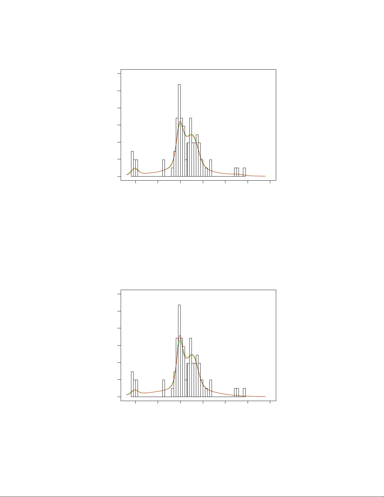
Perfect Simulation for Mixtures with Kno wn and Unkno wn Number of Components Sabyasachi Mukhopadhyay and Sourabh Bhattacharya ∗ Abstract W e propose and de velop a no vel and effecti ve perfect sampling methodology for simulating from posteriors corresponding to mixtures with either kno wn (fixed) or unknown number of components. For the latter we consider the Dirichlet process-based mixture model developed by these authors, and sho w that our ideas are applicable to conjugate, and importantly , to non- conjugate cases. As to be expected, and as we sho w , perfect sampling for mixtures with known number of components can be achie ved with much less effort with a simplified v ersion of our general methodology , whether or not conjugate or non-conjugate priors are used. While no special assumption is necessary in the conjugate set-up for our theory to work, we require the assumption of compact parameter space in the non-conjugat e set-up. Ho wev er, we argue, with appropriate analytical, simulation, and real data studies as support, that such compactness assumption is not unrealistic and is not an impediment in practice. Not only do we validate our ideas theoretically and with simulation studies, b ut we also consider application of our proposal to three real data sets used by several authors in the past in connection with mixture models. The results we achiev ed in each of our experiments with either simulation study or real data application, are quite encouraging. Ho wever , the computation can be extremely burdensome in the case of large number of mixture components and in massi ve data sets. W e discuss the role of parallel processing in mitigating the extreme computational b urden. K eywor ds: Bounding chains; Dirichlet process; Gibbs sampling; Mixtures; Optimization; Per- fect Sampling ∗ Sabyasachi Mukhopadhyay is a PhD student and Sourabh Bhattacharya is an Assistant Professor in Bayesian and Interdisciplinary Research Unit, Indian Statistical Institute, K olkata, India. Corresponding e-mail: sourabh@isical.ac.in 1 1. INTR ODUCTION Marko v chain Monte Carlo (MCMC) algorithms are de veloped to simulate from desired distribu- tions, from which generation of exact samples is difficult. The methodology has found much use in the Bayesian statistical paradigm thanks to the natural need to sample from intractable posterior distributions. But in whatev er clev er way the MCMC algorithms are designed, t he samples are gen- erated only approximately . Due to impossibility of running the chain for an infinite span of time, a suitable burn-in period is chosen, usually by a combination of empirical and ad-hoc means. The realizations retained after discarding the burn-in period are presumed to closely represent the true distribution. The degree of closeness, howe ver , depends upon ho w suitably the burn-in is chosen, and an arbitrary choice may lead to serious bias. Even in simple problems non-negligible biases often result if the burn-in period is chosen inadequately (see, for example, Roberts & Rosenthal (1998)). Such problems can only be aggrav ated in the case of realistic, more complex models, such as mixture models of the form, gi ven for the data point y , by [ y | Θ p , Π p ] = p X j =1 π j f ( y | θ j ) , (1) In (1), Θ p denotes the set of parameters ( θ 1 , . . . , θ p ) 0 , Π p = ( π 1 , . . . , π p ) 0 are the mixing probabili- ties such that π j > 0 for j = 1 , . . . , p , and P p j =1 π j = 1 . Here the number of mixture components p may or may not be known. The latter case corresponds to variable dimensional parameter space since the cardinality of the set Θ p then becomes random. Mixture models form a very important class of models in statistics, kno wn for their versatil- ity . The Bayesian paradigm ev en allo ws for random number of mixture components (making the dimensionality of the parameter space a random variable), adding to the flexibility of mixture mod- els. Sophisticated MCMC algorithms are needed for posterior inference in mixture models, raising the question of adequacy of the av ailable practical con ver gence assessment methods, particularly in the case of variable-dimensional mixture models. The importance of the aforementioned class of models makes it important to solve the associated con ver gence assessment problem. In this paper , we de velop a rigorous solution to this problem using the principle of perfect sampling. The perfect sampling methodology , first proposed in the seminal paper by Propp & W ilson 2 (1996), attempts to completely av oid the problems of MCMC con ver gence assessment. In prin- ciple, starting at all possible initial v alues, so many parallel Marko v chains need to be run, each starting at time t = −∞ . If by time t = 0 , all the chains coalesce, the coalescent point at time t = 0 is an e xact realization from the stationary distrib ution. Essentially , this principle works in the same way as the regular MCMC algorithms, but by replacing its starting time t = 0 with t = −∞ and the con ver gence time t = ∞ with t = 0 . T o achiev e perfect sampling in practice, Propp & W ilson (1996) proposed the “coupling from the past” (CFTP) algorithm, which avoids running Marko v chains from the infinite past. W e briefly describe this in the next section. 2. THE CFTP ALGORITHM For the time being, for the sak e of clarity , following Propp & W ilson (1996), let us assume that the state space X is finite, and let { X t ; t = 0 , 1 , . . . } denote the underlying Marko v chain. Then, for t ≥ 0 it is possible to represent the Markov chain generically as a random mapping: X t +1 = φ t ( X t ) = φ ( X t , R t +1 ) , for some function φ ( · , · ) and an iid sequence { R t ; t = 1 , . . . } . Then the CFTP algorithm is as follo ws (see Propp & W ilson (1996), Robert & Casella (2004)): 1. For t = − 1 , − 2 , . . . , generate φ t ( x ) for x ∈ X . 2. For t = − 1 , − 2 , . . . , for x ∈ X , define the compositions Φ t ( x ) = φ 0 ◦ φ − 1 ◦ · · · φ − t ( x ) (2) 3. Determine the time T such that Φ T is constant. 4. Accept Φ T ( x ∗ ) as an exact realization from the stationary distrib ution for an y arbitrary x ∗ ∈ X . It is well-kno wn (see, for e xample, Casella, La vine & Robert (2001)) that the abo ve algorithm terminates almost surely in finite time under very mild conditions and indeed yields a realization distributed exactly according to the stationary distrib ution of the Marko v chain. Propp & W ilson (1996) recommend taking t = − 2 j , for j = 1 , 2 , . . . , which we shall adopt in this paper . A 3 subtle, b ut important point is that, ev en if all the Markov chains coalesce before time t = 0 , the corresponding simulation at the time of coalescence need not yield a perfect sample. One needs to carry the algorithm forward till time t = 0 ; the sample corresponding to only t = 0 is guaranteed to be perfect. For details, see Casella et al. (2001). Although in the seminal paper of Propp & W ilson (1996) the CFTP algorithm, as described abov e, was constructed assuming finite state space in the above algorithm, later dev elopments managed to circumv ent this assumption of finiteness. Indeed, strategies for perfect sampling in general state spaces are described in Murdoch & Green (1998) and Green & Murdoch (1999), but quite restricted set-ups, which do not hold generally , are needed to implement such strategies. The set up of mixture models is much complex, and the kno wn strategies are dif ficult to apply . The first attempt to construct perfect sampling algorithms for mixture models is by Hobert, Robert & T itterington (1999). Howe ver , the y assumed only 2-component and 3-component mix- ture models, where only the mixing probabilities are assumed to be unkno wn. Bounding chains (this term seems to first appear in Huber (1998); Huber (2004) also uses this term) with mono- tonicity structures are used to enable the CFTP algorithm in these cases. Using the principle of the perfect slice sampler (Mira, Møller & Roberts (2001)), and assuming conjugate priors on the pa- rameters, Casella, Mengersen, Robert & T itterington (2002) proposed a perfect sampling method- ology for mixtures with known number of components by marginalizing out the parameters. It is noted in Casella et al. (2002) that in the conjugate case the marginalized form of the posterior is an- alytically av ailable, but the authors point out (see Section 2 of Casella et al. (2002)) that still perfect simulation from the analytically av ailable marginalized posterior is important. Unfortunately , apart from the somewhat restricted assumptions of conjugate priors and known number of components, the methodology is approximate in nature and the authors themselves demonstrated that the ap- proximation can be quite poor . Fearnhead (2005) proposed a direct sampling methodology based on recursion relations associated with the forward-backward algorithm, for mixtures of discrete distributions assuming a conjugate set-up and known number of components, thus bringing in an extra and crucial assumption of discrete data. Most recently , Berthelsen, Breyer & Roberts (2010) introduced a new perfect sampling methodology in mixtures with known number of components 4 where only the mixture weights are unknown. The method is also shown to work for normal mix- tures (with kno wn number of components) with unknown weights as well as with unknown means, but with a known, common v ariance. Ho wev er , ev en in this much restricted setup, the practicality of the algorithm is challenged. Indeed, the authors honestly remarked in pages 255–256 the fol- lo wing: “Unfortunately , in practice this extension of our algorithm seems to be feasible only for fairly small data sets ( n < 5) where the data consist of one cluster . ” Ho wev er , the drawbacks of the methodologies in no w ay present the contrib utions of the afore- mentioned authors in poor light, these only show ho w difficult the problem is. In this paper we at- tempt to av oid the restrictions and dif ficulties by proposing a novel approach. In the non-conjugate case (but not in the conjugate case) we are forced to assume compactness of the parameter space, but we argue in Section 3.3, followed up with a simulated data example in the supplement and three real data cases in Section 5, that it is not an unrealistic assumption, particularly in the Bayesian paradigm. Noting particularly that no methodology exists in the literature that ev en attempts per - fect simulation from mixtures with unkno wn number of components, for either compact or non- compact parameter space, for either conjugate or non-conjugate set-up, there is no reason to look upon our compactness assumption only in the non-conjugate case as a serious drawback. W e first construct a perfect sampling algorithm for mixture models with fixed (known) number of components and then generalize the ideas to mixtures with unknown number of components. For the sake of illustration, we concentrate on mixtures of normal densities, but our ideas are quite generally applicable. W e illustrate our methodology with simulation studies as well as with application to three real data sets. Additional technical details and further details on experiments are provided in the supplement, whose sections and figures have the prefix “S-” when referred to in this paper . 5 3. PERFECT SAMPLING FOR NORMAL MIXTURES WITH KNO WN NUMBER OF COMPONENTS 3.1 Normal mixture model and prior distributions Letting f ( · | θ j ) in (1) denote normal densities with mean µ j and variance σ 2 j , we obtain the follo wing normal mixture model [ y | Θ p , Π p ] = p X j =1 π j r λ j 2 π exp  − λ j 2 ( y − µ j ) 2  , (3) In (3), θ j = ( µ j , λ j ) , where λ j = σ − 2 j . For the sak e of conv enience of illustration only we consider the follo wing conjugate prior specification on the unknown v ariables λ j iid ∼ Gamma ( η / 2 , ζ / 2); j = 1 , . . . , p (4) [ µ j | λ j ] iid ∼ N ( ξ j , τ 2 j λ − 1 j ); j = 1 , . . . , p (5) Π p = ( π 1 , . . . , π p ) ∼ D irichl et ( γ 1 , . . . , γ p ) (6) (7) In (4), Gamma ( η / 2 , ζ / 2) denotes the Gamma distribution with density proportional to λ η / 2 − 1 j exp {− ζ λ j / 2 } . W e further assume that { η , ζ } , { ξ 1 , . . . , ξ p } , { τ 1 , . . . , τ p } and { γ 1 , . . . , γ p } are kno wn. W ith conjugate priors the marginal posteriors of the parameters (Π p , Θ p ) and the allocation v ariables Z are av ailable in closed forms, but still sampling from the posterior distributions is im- portant. Indeed, Casella et al. (2002) argue that sampling enables inference on arbitrary functionals of the unkno wn variables, which are not analytically av ailable. These authors proposed a perfect slice sampler for sampling from the mar ginal posterior of the allocation v ariable Z only . Gi ven perfect samples from the posterior of Z , drawing exact samples from the posterior distributions of (Π p , Θ p ) is straightforward. But importantly , the posteriors are not av ailable in closed forms in non-conjugate situations, and ev en Gibbs sampling is not straightforward in such cases. Since our goal is to provide a general theory that works for both conjugate and non-conjugate priors, we do not focus on the mar ginalized approach, although the conjugate situation is just a special (and sim- pler) case of our proposed principle (see Sections 3.3 and 4.5). Due to con venience of illustration 6 we begin with the conjugate prior case where the full conditional distrib utions needed for Gibbs sampling are av ailable. It will be shown how the same ideas are carried over to the non-conjugate cases. 3.2 Full conditional distributions Assuming that a dataset Y = ( y 1 , . . . , y n ) 0 is av ailable, let us define the set of allocation variables Z = ( z 1 , . . . , z n ) 0 , where z i = j if y i comes from the j -th component of the mixture. Further, defining n j = # { i : z i = j } , ¯ y j = P i : z i = j y i /n j , Z − i = ( z 1 , . . . , z i − 1 , z i +1 , . . . , z n ) 0 and Θ − j p = ( θ 1 , . . . , θ j − 1 , θ j +1 , . . . , θ p ) 0 , the full conditional distributions of the unknown random variables can be expressed as the follo wing: [ z i = j | Θ p , Z − i , Π , Y ] ∝ π j p λ j exp  − λ j 2 ( y i − µ j ) 2  (8) [ λ j | Z, Π , Θ − j p , µ j , Y ] ∼ Gamma   η + n j 2 , 1 2    ζ + n j ( ¯ y j − ξ j ) 2 n j τ 2 j + 1 + X i : z i = j ( y i − ¯ y j ) 2      (9) [ µ j | Θ − j p , λ j , Z, Π , Y ] ∼ N   n j ¯ y j τ 2 j + ξ j n j τ 2 j + 1 , τ 2 j λ j  n j τ 2 j + 1    (10) [Π | Z, Θ , Y ] ∼ D irichl et ( n 1 + γ 1 , . . . , n p + γ p ) (11) Perfect sampling, making use of the full conditional distributions av ailable for Gibbs sampling, has been de veloped by Møller (1999). But the dev elopment is based on the assumption that the random variables are discrete and that the distribution functions are monotonic in the conditioned v ariables. These are not satisfied in the case of mixtures. Full conditional based perfect sampling has also been used by Schneider & Corcoran (2004) in the context of Bayesian variable selection in a linear regression model, but their methods depend strongly on the underlying structure of their linear regression model and prior assumptions and do not apply to mixture models. Our proposed method hinges on obtaining stochastic lo wer and upper bounds for the Z -part of the Gibbs sampler , and simulating only from the two bounding chains, and noting their coalescence. It turns out that, in our methodology , there is no need to simulate the other unkno wns, (Π p , Θ p ) before coalescence, e ven in the non-conjugate set-up. Details are provided in the next section. 7 3.3 Bounding chains for Z For i = 1 , . . . , n , let F i ( · | Y , Z − i , Π p , Θ p ) denote the distribution function corresponding to the full conditional of z i . Writing X − i = ( Z − i , Π p , Θ p ) , let F L i ( · | Y ) = inf X − i F i ( · | Y , X − i ) (12) F U i ( · | Y ) = sup X − i F i ( · | Y , X − i ) (13) be the lo wer and the upper bounds of F i ( · | Y , Z − i , Π p , Θ p ) . Note that the full conditional of z i , gi ven by (8), is independent of Z − i ; hence supremum or infimum ov er Z − i are not necessary . By enforcing bounds on (Π p , Θ p ) the infimum and the supremum in (12) and (13) can be made to be bounded a way from 0 and 1 for points whose distrib ution functional v alues a priori were bounded aw ay from 0 and 1. Also, (12) and (13) will take the v alues 0 or 1 for the points which had, respecti vely , distributional functional v alues 0 or 1 a priori . In other words, there is a single set of points recei ving positi ve masses under the probability mass functions associated with both (12) and (13), which we subsequently prov e to be distrib ution functions. This set is also exactly the same set of points receiving positi ve masses under the probability mass function corresponding to the distribution function a priori . Thus, the support of Θ p would be compact, and that of Π p would be a compact subset of its original support. This is not an unrealistic assumption since in all practical situations, parameters are essentially bounded away from the extreme values. In fact, the prior on the parameters is expected to contain at least the information re garding the range of the parameters. In almost all practical applications, this range is finite, which, in principle, is possible to elicit. W e believ e that non-compact parameter spaces are assumed only due to the associated analytic adv antages (for instance, generally integrals are easier to ev aluate analytically under the full support) and because of the difficulty in v olved in elicitation of proper priors with truncated support. Ho wev er , we show in Section S-11.3, that truncation of the support of Π p need not always be necessary . In order to decide upon some adequate compact support, a pilot Gibbs sampling run with un- bounded Θ p may be implemented first, and then the effecti ve range of the posterior of Θ p can be chosen as the compact support of the prior of Θ p . This range may be further refined by subse- 8 quently running a Gibbs sampler with the chosen compact support, comparing the resultant density with that corresponding to the unbounded support, and, if necessary , modifying the chosen range so that the densities agree with each other as closely as possible. It is demonstrated with simulated examples in Sections S-11.3, 4.6, and with three real applications in Sections 5.1, 5.2, and 5.3 that often the posterior with unbounded support is almost the same as that with compact support, obtained from pilot Gibbs sampling. Unless otherwise mentioned, throughout we assume compact support of Θ p . W e remark here that the compactness assumption is not needed in the case of con- jugate prior on Θ p . In that case, Θ p will be inte grated out analytically , and hence (12) and (13) will not in volv e Θ p , thus simplifying proceedings. Had the minimizer and the maximizer of F i ( j | Y , X − i ) with respect to X − i been constant with respect to j , then, trivially , (12) and (13) would hav e been distribution functions. But this is not the case unless z i takes on only two v alues with positi ve probability , as in the case of 2-component mixture models. Howe ver , as sho wn in Section S-7, F L i ( · | Y ) and F U i ( · | Y ) satisfy the properties of distrib ution functions for any discrete random v ariable. So, their in versions will sandwich all possible realizations obtained by in verting F i ( · | Y , X − i ) , irrespecti ve of any X − i . T o clarify the sandwiching argument, we first define the in verse of any distrib ution function F by F − ( x ) = inf { y : F ( y ) ≥ x } . Further , let R Z,t = { R z i ,t ; i = 1 , . . . , n } be a common set of iid random numbers used to simulate Z at time t for Markov chains starting at all possible initial v alues. If we define z it = F i − ( R z i ,t | Y , X − i ) , z L it = F U i − ( R z i ,t | Y ) and z U it = F L i − ( R z i ,t | Y ) , then, for all possible X − i , it holds that z L it ≤ z it ≤ z U it for i = 1 , . . . , n and t = 1 , 2 , . . . . These imply that once all z i ; i = 1 , . . . , n , dra wn by in verting F L i and F U i coalesce, then so will e very realization of Z drawn from F i ( · | X − i ) , for i = 1 , . . . , n , starting at all possible initial values. Analogous to { R Z,t ; t = 1 , 2 , . . . } , let { R Π p ,t ; t = 1 , 2 , . . . } and { R Θ p ,t ; t = 1 , 2 , . . . } denote sets of iid random numbers needed to generate Π p and Θ p , respecti vely , in a hypothetical CFTP algorithm, where Markov chains from all possible starting values are simulated, with Z updated first. Once Z coalesces, so will (Π p , Θ p ) since their full conditionals (see (9), (10) and (11)) show that the corresponding deterministic random mapping function depends only upon Z , { R Π p ,t ; t = 1 , 2 , . . . } , and { R Θ p ,t ; t = 1 , 2 , . . . } . W e remark here that the random numbers can always be 9 thought of as realizations of U nif or m (0 , 1) , since the deterministic random mapping function can always be represented in terms of U nif or m (0 , 1) random numbers. The ke y idea is illustrated algorithmically below . Algorithm 3.1 CFTP for mixtur es with known number of components (i) For i = 1 , . . . , n , and for ` = 1 , . . . , p , calculate F L i ( ` | Y ) and F U i ( ` | Y ) , gi ven by (12) and (13) using some ef ficient optimization method. W e recommend simulated annealing; see Section 3.7. (ii) For j = 1 . . . , until coalescence of Z , repeat steps (iii) and (iv) belo w . (iii) Define S j = {− 2 j + 1 , . . . , − 2 j − 1 } for j ≥ 2 , and let S 1 = {− 1 , 0 } . For each m ∈ S j , generate random numbers R Z,m , R Π p ,m and R Θ p ,m from U nif or m (0 , 1) ; once generated, treat them as fixed thereafter for all iterations. It is important to note that at step − 2 j no random number generation is required since that step can be viewed as the initializing step, where all possible chains, from all possible initial v alues of Z , Π p , and Θ p , are started. (i v) For t = − 2 j + 1 , . . . , − 1 , 0 , determine z L it = F U − i ( R z i,t | Y ) and z U it = F L − i ( R z i,t | Y ) ∀ i = 1 , . . . , n . This step can be thought of as initializing the perfect sampler with all pos- sible values of Z and (Π p , Θ p ) at step − 2 j , and then moving on to the next forward step follo wing generation of Z independently of the pre vious step, using the abov e random num- bers and optimized distribution functions. Generation of (Π p , Θ p ) is not necessary because of the sandwiching relation z L it ≤ z it ≤ z U it , which holds for any (Π p , Θ p ) , and because co- alescence of z L it and z U it ∀ i = 1 , . . . , n for some t ≤ 0 guarantees coalescence of all chains corresponding to (Π p , Θ p ) . (v) If z L it ∗ = z U it ∗ ∀ i = 1 , . . . , n and for some t ∗ < 0 , then run the following Gibbs sampling steps from t = t ∗ to t = 0 : (a) Let Z ∗ = ( z ∗ 1 , . . . , z ∗ n ) 0 denote the coalesced v alue of Z at time t ∗ . Giv en Z ∗ , draw (Π ∗ p , Θ ∗ p ) from the full conditionals (11), (9) and (10) in order , using the corresponding 10 random numbers already generated. Thus, ( Z ∗ , Π ∗ p , Θ ∗ p ) is the coalesced v alue of the unkno wn quantities at t = t ∗ . Importantly , it is not straightforward to sample from full conditionals of non-conjugate distributions and/or in the case of compact param- eter spaces. In such situations we recommend rejection sampling/adaptiv e rejection sampling; see Section 3.5 for details. (b) Carry forward the abov e Gibbs sampling chain started at t = t ∗ till t = 0 , simulating sequentially from (8), (11), (9) and (10). Then, the output of the Gibbs sampler ob- tained at t = 0 , which we denote by ( Z 0 , Π p 0 , Θ p 0 ) , is a perfect sample from the true target posterior distrib ution. Note that here optimization is required only once, in Step (i) of Algorithm 3.1. By reducing the gaps between the bounding chains, the algorithm can be made further ef ficient. Such techniques are discussed in Section 3.4 in conjunction with Section S-11. In fact, we present a variant of the abov e algorithm for two-component mixtures in Algorithm S-11.1 where optimization with respect to the mixture component probability is not required. That algorithm exploits a monotonicity structure which is not enjoyed by mixtures having more than two components. Indeed, e ven though Algorithm 3.1 is applicable for mixtures with any known number of components, Algorithm S-11.1 is applicable only to two-component mixtures. It is interesting to note that we need to run just two chains (12) and (13) and check their coalescence; there is no need to simulate (Π p , Θ p ) before coalescence occurs with respect to Z in these two bounding chains, even in non-conjugate cases. This property of our methodology has some important adv antages which are detailed in Section 3.6. It is prov ed in Section S-8 that coalescence of Z occurs almost surely in finite time. Foss & T weedie (1998) sho wed that coalescence occurs in finite time if and only if the underlying Marko v chain is uniformly ergodic. In Section S-9 we sho w that our Gibbs sampler , which first updates Z , is uniformly ergodic, which is expected thanks to the compact parameter space. The proofs in Sections S-7, S-8 and S-9 go through with the modified bounds needed for mixtures with unkno wn number of components. 11 In conjugate setups further simplification results since we only need to simulate perfectly from the posterior of Z ; once a perfect sample of Z is obtained, simulations from (11), (9), and (10) ensures e xact samples from the posteriors of (Π p , Θ p ) as well. In order to simulate from the poste- rior of Z , we can integrate out (Π p , Θ p ) from the full conditional of z i and construct the bounding chains with respect to the marginalized distribution function of z i , optimizing the marginalized distribution function with respect to Z − i . 3.4 Ef ficiency of the bounding chains It is an important question to ask if the lower bound (12) can be made larger or if the upper bound (13) can be made smaller , to accelerate coalescence. This can be achie ved if a monotonicity structure can be identified in (Π p , Θ p ) . In Section S-11 we illustrate this with an example. In Section 4.5 we propose a method for reducing the gaps between the bounds in mixture models with unkno wn number of components. There it is also discussed that for these models, more information in the data can further reduce the gap between the bounding chains. 3.5 Restricted parameter space and rejection sampling after coalescence If our algorithm coalesces at time t < 0 , then Gibbs sampling is necessary from that point on till time t = 0 . The bounds, howe ver , may prev ent exact simulation from the full conditionals of Θ p using con ventional methods, such as the Box-Muller transform ation (Box & Muller (1958)) in the case of normal full conditionals, which becomes truncated normal under the restrictions. In these situations, rejection sampling may be used. Briefly , let { R ∗ rt ; r = 1 , 2 , . . . } denote a collection of infinite random numbers, to be used sequentially for rejection sampling of the continuous random v ariables at time t by the full conditionals of the continuous random variables. Actual simulation using rejection sampling is not necessary until Z coalesces. In the case of non-conjugate priors (perhaps, in addition to restricted parameter space), the full conditional densities are often log- concav e. In such situations the same principle can be used, but with rejection sampling replaced by adapti ve rejection sampling (Gilks & W ild (1992), Gilks (1992)). 12 3.6 Adv antages of our approach Our bounding chain approach for only the discrete components Z has sev eral advantages ov er the pre vious approaches. Firstly , simulation of the continuous parameters before coalescence of Z , is unnecessary . This adv antage is important because construction of bounds for the continuous parameters, e ven if possible, may not be useful since the coalescence probability of continuous parameters corresponding to the bounding chains, is zero. Moreov er , bounding the distribution functions of continuous parameters in the mixture model context does not seem to be straightfor- ward without discretization. Another adv antage of our perfect sampling principle is that we do not need a partial order of the multi-dimensional state space and it is unnecessary to find minimal and maximal elements to serve as initial values of the bounding chains. Indeed, our bounding chains begin with simulations from F L 1 ( · | Y ) and F U 1 ( · | Y ) , which do not require any initial v alues. Also, importantly , our approach of creating bounds for Z does not depend upon the assumption of conjugate priors. Exactly the same approach will be used in the case of non-conjugate priors. After coalescence, regardless of compact support or non-conjugate priors, Gibbs sampling can be carried out in a very straightforw ard manner till time t = 0 . 3.7 Obtaining infimum and supremum of F i ( · | Y , X − i ) in practice For each j = 1 , . . . , p , and for all i = 1 , . . . , n , the bounds F L i ( j | Y ) and F U i ( j | Y ) are bounded aw ay from 0 and 1 but not always easily av ailable in closed forms. Numerical optimization using simulated annealing (see, for e xample, Robert & Casella (2004) and the references therein) with temperature T ∝ 1 log(1+ t ) , where t is the iteration number , turned out to be v ery effecti ve in our case. This is because the method, when properly tuned, can be quite accurate, and it is entirely straightforward to handle constraints (introduced through the restricted parameter space in our methodology) with simulated annealing through the acceptance-rejection steps as in Metropolis- Hastings algorithm. At each time t a set of fix ed random numbers will be used for implementation of simulated annealing within our perfect sampling methodology . Interestingly , for our perfect sampling algorithm we do not need simulated annealing to be arbitrarily accurate; gi ven random numbers { R Z,t ; t = 1 , 2 , . . . } we only need it to be accurate 13 enough to generate the same realization from the approximated distribution functions as obtained had we used the exact solution. For instance, assume that F L i ( j − 1 | Y ) < R z i ,t ≤ F L i ( j | Y ) , implying that z L it = j . Letting ˆ F L i denote the approximated distribution function, we only need the approximation to satisfy ˆ F L i ( j − 1 | Y ) < R z i ,t < ˆ F L i ( j | Y ) so that z L it = j ev en under the approximation. This is achiev able e ven if arbitrarily accurate approximation is not obtained. Since in general there seems to be no way to check the error of approximation by simulated annealing, we propose the following method. Instead of a single run of simulated annealing with a fixed run length, one may gi ve a fe w more runs, in each case increasing the length of the run by a moderately large integer , and obtain z L it and z U it in each case. Since the random numbers R Z,t are fix ed (in fact, we recommend fixing the random numbers used for simulated annealing as well), the v alues of z L it and z U it will become constants as the run length increases for simulated annealing. These constants must be the same as would ha ve been obtained had the optimization been exact. This strate gy is not excessi vely b urdensome computationally , since there is no need to carry out each run afresh; the output of the last iteration of the current run of simulated annealing will be taken as the initial v alue for the next run. Our perfect sampling methodology is illustrated in a 2-component normal mixture e xample in Section S-11; here we simply note that our method work ed excellently . A further e xperiment associated with the same example, and reported in Section S-11.4, showed that perfect sampling based on simulated annealing yielded results exactly the same as those obtained by perfect sam- pling based on exact optimization, in 100% of 100,000 cases. The outcome of the latter experiment clearly encourages the use of simulated annealing for optimization in perfect sampling. W e now e xtend our perfect sampling methodology to mixtures with unknown number of com- ponents, which is a v ariable-dimensional problem. In this context, the non-parametric approach of Escobar & W est (1995) and the re versible jump MCMC (RJMCMC) approach of Richardson & Green (1997) are pioneering. The former uses Dirichlet process (see, for example, Fer guson (1974)) to implicitly induce v ariability in the number of components, while maintaining a fix ed- dimensional frame work, while the latter directly treats the number of components as unkno wn, dealing directly , in the process, with a v ariable dimensional framework. The comple xities in volved 14 with the latter frame work mak es it dif ficult to extend our perfect sampling methodology to the case of RJMCMC. A ne w , flexible mixture model based on Dirichlet process has been introduced by Bhattacharya (2008) (henceforth, SB), which is sho wn by Mukhopadhyay , Bhattacharya & Dihidar (2011) (see also Mukhopadhyay , Roy & Bhattacharya (2012)) to include Escobar & W est (1995) as a special case, and is much more efficient and computationally cheap compared to the latter . Hence, we dev elop a perfect sampling methodology for the model of SB, which automatically applies to Escobar & W est (1995). 4. PERFECT SAMPLING FOR NORMAL MIXTURES WITH UNKNO WN NUMBER OF COMPONENTS As before, let Y = ( y 1 , . . . , y n ) 0 denote the av ailable data set. SB considers the following model [ y i | Θ M ] ∼ 1 M M X j =1 r λ j 2 π exp  − λ j 2 ( y i − µ j ) 2  (14) In the abov e, M is the maximum number of components the mixture can possibly ha ve, and is kno wn; Θ M = { θ 1 , θ 2 , . . . , θ M } with θ j = ( µ j , λ j ), where λ j = σ − 2 j . W e further assume that Θ M are samples drawn from a Dirichlet process: θ j iid ∼ G G ∼ D P ( α G 0 ) (15) Usually a Gamma prior is assigned to the scale parameter α . Under the mean distribution G 0 in (15), λ j iid ∼ Gamma  η 2 , ζ 2  (16) [ µ j | λ j ] ∼ N ( µ 0 , ψ λ − 1 j ) (17) Under the Dirichlet process assumption the parameters θ j are coincident with positiv e proba- bility; because of this (14) reduces to the form [ y i | Θ M ] = p X j =1 π j r λ ∗ j 2 π exp  − λ ∗ j 2 ( y i − µ ∗ j ) 2  , (18) 15 where  θ ∗ 1 , . . . , θ ∗ p  are p distinct components in Θ M with θ ∗ j occurring M j times, and π j = M j / M . Using allocation v ariables Z = ( z 1 , . . . , z n ) 0 , SB’ s model can be represented as follo ws: For i = 1 , . . . , n and j = 1 , . . . , M , [ y i | z i = j, Θ M ] = r λ j 2 π exp  − λ j 2 ( y i − µ j ) 2  (19) [ z i = j ] = 1 M (20) As is easily seen and is ar gued in Mukhopadhyay et al. (2012), setting M = n and z i = i for i = 1 , . . . , M (= n ) , that is, treating Z = (1 , 2 , . . . , n ) 0 as non-random, yields the Dirichlet process mixture model of Escobar & W est (1995). Ho wev er , unlike the case of mixtures with fixed number of components, the full conditionals of only Z and Θ M can not be used to construct an efficient perfect sampling algorithm in the case of unkno wn number of components. This is because the full conditional of θ j gi ven the rest depends upon Z as well as Θ − j M , which implies that e ven if Z coalesces, θ j can not coalesce unless Θ − j M also coalesces. But this has v ery little probability of happening in one step. Of more concern is the fact that Z may again become non-coalescent if Θ M does not coalesce immediately after Z coalesces. Hence, although the algorithm will ultimately con verge, it may take too many iterations. This problem can be bypassed by considering the reparameterized version of the model, based on the distinct elements of Θ M and the configuration indicators. 4.1 Reparameterization using configuration indicators and associated full conditionals As before we define the set of allocation v ariables Z = ( z 1 , . . . , z n ) 0 , where z i = j if y i is from the j -th component. Letting Θ ∗ M = { θ ∗ 1 , . . . , θ ∗ k } denote the distinct components in Θ M , the element c j of the configuration v ector C = ( c 1 , . . . , c M ) 0 is defined as c j = ` if and only if θ j = θ ∗ ` ; j = 1 , . . . , M , ` = 1 , . . . , k . Thus, ( Z, Θ M ) is reparameterized to ( Z, C , k , Θ ∗ M ) , k denoting the number of distinct components in Θ M . The full conditional distribution of z i is gi ven by [ z i = j | Y , C , k , Θ ∗ M ] ∝ r λ j 2 π exp  − λ j 2 ( y i − µ j ) 2  (21) 16 Since Θ M can be obtained from C and Θ ∗ M , we represented the right hand side of (21) in terms of Θ M . T o obtain the full conditional of c j , first let k j denote the number of distinct values in Θ − j M , and let θ j ∗ ` ; ` = 1 , . . . , k j denote the distinct v alues. Also suppose that θ j ∗ ` occurs M `j times. Then the conditional distribution of c j is gi ven by [ c j = ` | Y , Z , C − j , k j , Θ ∗ M ] =    κq ∗ `j if ` = 1 , . . . , k j κq 0 j if ` = k j + 1 (22) where q 0 j = α ( ζ 2 ) η 2 Γ( η 2 ) ×  1 n j ψ + 1  1 2 ×  1 2 π  n j 2 × 2 η + n j 2 Γ( η + n j 2 ) n ζ + n j ( ¯ y j − µ 0 ) 2 n j ψ +1 + P i : z i = j ( y i − ¯ y j ) 2 o η + n j 2 , (23) q ∗ `j = M `j ( λ j ∗ ` ) n j 2 (2 π ) n j 2 exp " − λ j ∗ ` 2 ( n j ( µ j ∗ ` − ¯ y j ) 2 + X i : z i = j ( y i − ¯ y j ) 2 )# (24) In (22), (23), and (24), κ is the normalizing constant, n j = # { i : z i = j } and ¯ y j = P i : z i = j y i /n j . Note that q 0 j is the normalizing constant of the distribution G j defined by the follo wing: [ λ j ] ∼ Gamma η + n j 2 , 1 2 ( ζ + n j ( ¯ y j − µ 0 ) 2 n j ψ + 1 + X i : z i = j ( y i − ¯ y j ) 2 )! (25) [ µ j | λ j ] ∼ N  n j ¯ y j ψ + µ 0 n j ψ + 1 , ψ λ j ( n j ψ + 1)  (26) The conditional posterior distribution of θ ∗ ` is gi ven by [ θ ∗ ` | Y , Z , C ] ∼ Gamma ( λ ∗ ` : η ∗ ` , ζ ∗ ` ) × N  µ ∗ ` : µ ∗ 0 ` , ψ ∗ ` λ ∗ ` − 1  , (27) where n ∗ ` = X j : c j = ` n j , ¯ y ∗ ` = X j : c j = ` n j ¯ y j . X j : c j = ` n j , η ∗ ` = n ∗ ` + η 2 , (28) µ ∗ 0 ` = ( ψ n ∗ ` ¯ y ∗ ` + µ 0 ) / ( ψ n ∗ ` + 1) , (29) ψ ∗ ` = ψ  ( ψ n ∗ ` + 1) , (30) 17 and ζ ∗ ` = 1 2    ζ + n ∗ ` ( µ 0 − ¯ y ∗ ` ) 2 ψ n ∗ ` + 1 + X j : c j = ` n j ( ¯ y j − ¯ y ∗ ` ) 2 + X j : c j = ` X i : z i = j ( y i − ¯ y j ) 2    . (31) It is to be noted that the θ ∗ ` are conditionally independent. For Gibbs sampling, we first update Z , followed by updating C and the number of distinct components k , and finally { θ ∗ ` ; ` = 1 , . . . , k } . 4.2 Non-conjugate G 0 In the case of non-conjugate G 0 (which may hav e the same density form as a conjugate prior but with compact support), q 0 j is not av ailable in closed form. W e then modify our Gibbs sampling strategy by bringing in auxiliary variables in a way similar to that of Algorithm 8 in Neal (2000). T o clarify , let θ a = ( µ a , λ a ) denote an auxiliary variable (the superscript “ a ” stands for auxiliary). Then, before updating c j we first simulate from the full conditional distrib ution of θ a gi ven the current c j and the rest of the variables as follo ws: if c j = c ` for some ` 6 = j , then θ a ∼ G 0 . If, on the other hand, c j 6 = c ` ∀ ` 6 = j , then we set θ a = θ ∗ c j . Once θ a is obtained we then replace the intractable q 0 j with the tractable expression q a j = α ( λ a j ) n j 2 (2 π ) n j 2 exp " − λ a j 2 ( n j ( µ a j − ¯ y j ) 2 + X i : z i = j ( y i − ¯ y j ) 2 )# (32) Once c j is simulated, if it is observed that θ j 6 = θ a ∀ j , then θ a is discarded. 4.3 Relabeling C Simulation of C by successiv ely simulating from the full conditional distributions (22) incurs a labeling problem. For instance, it is possible that all c j are equal e ven though each of them cor- responds to a distinct θ j . For an e xample, suppose that Θ ∗ M consists of M distinct elements, and c j = M ∀ j . Then although there are actually M distinct components, one ends up obtaining just one distinct component. For perfect sampling we create a labeling method which relabels C such that the relabeled version, which we denote by S = ( s 1 , . . . , s M ) 0 , coalesces if C coalesces. T o construct S we first simulate c j from (22); if c j ∈ { 1 , . . . , k j } , then we set θ j = θ ∗ c j and if 18 c j = k j + 1 , we draw θ j = θ ∗ c j ∼ G j . The elements of S are obtained from the follo wing definition of s j : s j = ` if and only if θ j = θ ∗ ` . Note that s 1 = 1 and 1 ≤ s j ≤ s j − 1 + 1 . In Section S-10 it is proved that coalescence of C implies the coalescence of S , irrespective of the v alue of Θ ∗ M associated with C . 4.4 Full conditionals using S W ith the introduction of S it is now required to modify some of the full conditionals of the unknown random v ariables, in addition to introduction of the full conditional distribution of S . The form of the full conditional [ z i | Y , S, k , Θ ∗ M ] remains the same as (21), but Θ M in volv ed in the right hand side of (21) is no w obtained from S and Θ ∗ M . The modified full conditional of c j , which we denote by [ c j | Y , Z , S − j , k j , Θ ∗ M ] , now depends upon S − j , rather than C − j , the notation being clear from the context. The form of this full conditional remains the same as (22) but now the distinct components θ j ∗ ` ; ` = 1 , . . . , k j are associated with the corresponding components of S rather than C . The form of the modified full conditional distribution of θ ∗ ` , which we now denote by [ θ ∗ ` | Y , Z , S, k ] , remains the same as (27), but in equations (28) to (31), C must be replaced by S . In the abov e full conditionals, k and k j are no w assumed to be associated with S . The conditional posterior [ S | Y , C , Θ M ] giv es point mass to S ∗ , where S ∗ = ( s ∗ 1 , . . . , s ∗ M ) 0 is the relabeling obtained from C and Θ M follo wing the method described in Section 4.3. For the construction of bounds, the indi vidual full conditionals [ s j | Y , S − j , C , Θ M ] , gi ving full mass to s ∗ j , will be considered due to the con v enience of dealing with distribution functions of one v ariable. It follo ws that once Z and C coalesces, S and Θ ∗ M must also coalesce. In the next section we describe ho w to construct efficient bounding chains for Z , C and S . Bounding chains for S are not strictly necessary as it is possible to optimize the bounds for Z and C with respect to S , but the ef ficiency of the other bounding chains is impro ved, leading to an improved perfect sampling algorithm, if we also construct bounding chains for S . 19 4.5 Bounding chains As in the case of mixtures with known number of components, here also the idea of construct- ing bounding chains is associated with distribution functions of the discrete random v ariates, b ut here the bounding chains can be made efficient by fixing the already coalesced individual discrete v ariates while taking the supremum and the infimum of the distribution functions. Moreover , for informati ve data, the full conditional distributions of c j (hence, of s j ) will be similar giv en an y v alues of the conditioned variables; thus the difference between the supremum and the infimum of their distribution functions are expected to be small. This particular heuristic is reflected in the results of the application of our methodology to three real data sets in Section 5. Also, as noted in Section 3.3, ev en in the case of unknown number of components, Θ ∗ M can be analytically marginalized out in conjugate cases, simplifying optimization procedures. The full conditional distributions associated with our model, mar ginalized ov er Θ ∗ M in a conjugate case are provided in Mukhopadhyay et al. (2011). 4.5.1. Bounds for Z Let F z i ( · | Y , S , k , Θ ∗ M ) denote the distrib ution function of the full con- ditional of z i , and let F c j ( · | Y , S − j , k j , Θ ∗ M ) , F s j ( · | Y , S − j , C , Θ M ) stand for those of c j and s j , respecti vely . Also assume that −∞ < M 1 ≤ µ j ≤ M 2 < ∞ and 0 ≤ M 3 ≤ λ j ≤ M 4 < ∞ , for all j . Let ¯ S denote the set consisting of only those s j that ha ve coalesced, and let S − = S \ ¯ S consist of the remaining s j . Then F L z i  · | Y , ¯ S  = inf S − ,k, Θ ∗ M F z i ( · | Y , ¯ S , S − , k , Θ ∗ M ) (33) F U z i  · | Y , ¯ S  = sup S − ,k, Θ ∗ M F z i ( · | Y , ¯ S , S − , k , Θ ∗ M ) (34) Clearly , fixing ¯ S helps reduce the gap between (33) and (34). The infimum and the supremum abov e can be calculated by simulated annealing. For the proposal mechanism needed for simulated annealing with ¯ S held fixed, we selected s j ∈ S − uniformly from { 1 , . . . , s j − 1 + 1 } , where s j − 1 either belongs to ¯ S or has been selected uniformly from { 1 , . . . , s j − 2 + 1 } . Once S is proposed in this way , this determines k automatically . W e then propose θ ∗ 1 , . . . , θ ∗ k using normal random walk 20 proposals with approximately optimized v ariance. 4.5.2. Bounds for C Let ¯ Z denote the set of coalesced z i , and let Z − = Z \ ¯ Z consist of those z j that did not yet coalesce. Then F L c j  · | Y , ¯ S , ¯ Z  = inf S − ,k j ,Z − , Θ ∗ M F c j ( · | Y , ¯ S , S − , k j , ¯ Z , Z − , Θ ∗ M ) (35) F U c j  · | Y , ¯ S , ¯ Z  = sup S − ,k j ,Z − , Θ ∗ M F c j ( · | Y , ¯ S , S − , k j , ¯ Z , Z − , Θ ∗ M ) (36) Note that for ¯ S = ∅ , the supremum corresponds to k j = 1 and the infimum corresponds to k j = M − 1 . If ¯ S 6 = ∅ , the supremum is associated with k j = # ¯ S \{ s j } , the number of distinct components of ¯ S \{ s j } , and the infimum corresponds to the case where k j = #  ¯ S ∪ S −  \{ s j } , when all elements of S − are distinct. Thus, proposal mechanism of S − for simulated annealing is not necessary; manually setting all elements of S − to be equal for obtaining the supremum and manually setting all elements of S − to be distinct for obtaining the infimum are suf ficient, since the actual values of the elements of S are unimportant. This strategy dictates the number of distinct elements of Θ M , and their positions. The proposal mechanism for Θ ∗ M may be chosen to be the same as that used for obtaining the bounds for z i , while the elements of Z − may be proposed by drawing uniformly from { 1 , . . . , M } . 4.5.3. Bounds for S Letting ¯ C and C − = C \ ¯ C denote the sets of coalesced and the non- coalesced c j , the lo wer and the upper bounds for the distribution function of s j are F L s j  · | Y , ¯ C  = inf C − , Θ ∗ M F s j ( · | Y , ¯ C , C − , Θ ∗ M ) (37) F U s j  · | Y , ¯ C  = sup C − , Θ ∗ M F s j ( · | Y , ¯ C , C − , Θ ∗ M ) (38) For simplicity let us denote F s j ( · | Y , ¯ C , C − , Θ ∗ M ) by F s j ( · ) suppressing the conditioned v ari- ables. Since, gi ven C and Θ ∗ M , S is uniquely determined, F s j ( k ) = 0 or 1, for k = 1 , . . . , M . Thus, optimization of F s j ( k ) needs to be carried out extremely carefully because either the correct optimum or the incorrect optimum will be obtained, lea ving no scope for approximation. How- e ver , simulated annealing is unlikely to perform adequately in this situation. For instance, while 21 maximizing, a long sequence of iterations yielding F s j ( k ) = 0 does not imply that 1 is not the maximum. Similarly , a long sequence of 1’ s while minimizing may mislead one to believ e that 1 is the minimum. In other words, the algorithm does not exhibit gradual mov e tow ards the opti- mum, making con vergence assessment very difficult. So, we propose to construct functions h j ( · ) of F s j ( · ) ’ s and appropriate auxiliary v ariables such that the optimization of F s j ( · ) is embedded in the optimization of h j ( · ) , while av oiding the aforementioned problems by allowing gradual move to wards the optimum. Details are pro vided belo w . A mor e con venient optimizing function W e construct h j ( · ) as follows: h j ( W , F ) = M X i =1 w i  F s j ( i ) + w i 1 + w i  1 2 (39) where W = ( w 1 , . . . , w M ) denotes the vector of weights, F = ( F s j (1) , . . . , F s j ( M )) and P M j =1 w j = 1 with w j > 0 , ∀ j . Clearly , 0 < h j ( · ) < 1 . W e represent w j as w j = n j P M i =1 n i , where n i > 0 . W e use simulated annealing to optimize (39) with respect to ( W , C − , Θ ∗ M ) but let n k → ∞ with the iteration number while simulating other n i ; i 6 = k randomly from some bounded interval. This leads to optimization of F s j ( k ) , while av oiding the problems of naiv e simulated annealing. In our examples we took n k ∝ log (1 + t ) , where t is the iteration number . Optimizing strate gy Since S is just a relabeled version of C , the distrib ution functions of the full conditionals of c j and s j are optimized by the same Θ M , pro vided that none of s j coalesced during optimization in the case of C . All that the proposal mechanism requires then is to simulate c j ∈ C − uniformly from { 1 , . . . , M } . If C ( = ¯ C ∪ C − ) and Θ M do not lead to a valid S , then the proposal is to be rejected, remaining at the current C − , else the acceptance-rejection step of simulated annealing is to be implemented. If, on the other hand, some s j had coalesced during optimization in c j , the optimizer in the case of s j is expected to be a slight modification of that in the case of c j . W e construct the modification as follo ws. If C , simulated from the bounding chains (35) and (36) in the pre vious step, is not compatible with Θ M , then we augment Θ ∗ M with ne w components drawn uniformly: µ ∼ U ( M 1 , M 2 ) and λ ∼ U ( M 3 , M 4 ) , in such a manner that 22 compatibility is ensured. W e then use the adjusted set of Θ M for rest of the annealing steps. This scheme worked adequately in all our experiments. Note that if entire C coalesces, then for all j and for any Θ M associated with C , F L s j  · | Y , ¯ C  = F U s j  · | Y , ¯ C  = F s j ( · | Y , C , Θ M ) , which implies coalescence of S (recall the discussion in Section 4.4). The proof presented in Section S-7 goes through to show that the bounds of the distrib ution functions of ( Z , C , S ) , which are obtained by optimizing the original functions treating the coa- lesced random v ariates as fixed, are also distrib ution functions. The proof remains v alid ev en if the original distribution functions of the discrete variates are optimized with respect to the scale parameter α and other hyper -parameters. Optimization with respect to the latter is necessary if α and the hyper -parameters are treated as unknowns and must be simulated perfectly , like wise as Θ M . Assuming that the original Gibbs sampling algorithm is updated by first updating Z , then C , followed by S , and finally Θ ∗ M , the proof of coalescence of the random variables in finite time is e xactly as that provided in Section S-8. The proof of uniform er godicity presented in Section S-9 applies with minor modifications in the current mixture problem with unkno wn number of components. Belo w we provide an algorithmic representation of perfect sampling in mixtures with unkno wn number of components. Algorithm 4.1 CFTP for mixtur es with unknown number of components (1) For j = 1 . . . , until coalescence of ( Z, C ) , repeat steps (2) and (3) below . (2) Define S j = {− 2 j + 1 , . . . , − 2 j − 1 } for j ≥ 2 , and let S 1 = {− 1 , 0 } . For each m ∈ S j , generate random numbers R Z,m , R C,m , R S,m and R Θ M ,m (again, we shall let these random numbers stand for realizations from the uniform distrib ution on (0 , 1) ), meant for simulating Z , C , S , and Θ M respecti vely . Although random numbers are not necessary for simulating S from its optimized full conditionals because of degenerac y , R S,m will still be used for optimizing its distribution function using simulated annealing. The random numbers R Θ M ,m will correspond to M distinct components, so that the same set will suf fice for smaller num- bers of distinct components in the set Θ M where all components need not be distinct. The 23 distinct components of Θ M are meant to be simulated (b ut recall that actual simulation is not necessary until the coalescence of ( Z, C , S ) ) using those random numbers in the set R Θ M ,m , which correspond to their positions in Θ M . Once generated, treat the random numbers as fixed thereafter for all iterations. As in Algo- rithm 3.1, at step − 2 j no random number generation is required. (3) For t = − 2 j + 1 , . . . , − 1 , 0 , implement steps (3) (i), (3) (ii) and (3) (iii): (i) For i = 1 , . . . , n , (a) For ` = 1 , . . . , M , calculate F L z i ( ` | Y , ¯ S ) and F U z i ( ` | Y , ¯ S ) , using the simulated annealing method described in Section 4.5.1. (b) Determine z L it = F U − z i ( R z i,t | Y , ¯ S ) and z U it = F L − z i ( R z i,t | Y , ¯ S ) . As in Algorithm 3.1, this step can be thought of as initializing the perfect sampler with all possible v alues of ( Z, C , S, k , Θ ∗ M ) at step − 2 j ; at step − 2 j + 1 , ¯ S = ∅ (omitting the always coalescent s 1 = 1 ), signifying that simulations at this forward step is independent of the pre vious step − 2 j . From step − 2 j + 2 onwards, there is positi ve probability that ¯ S 6 = ∅ . Thus, with positi ve probability , the bounding chains for z i will be more ef ficient from this point on. (ii) For i = 1 , . . . , M , (a) For ` = 1 , . . . , k i + 1 , calculate F L c i ( ` | Y , ¯ S , ¯ Z ) and F U c i ( ` | Y , ¯ S , ¯ Z ) , using the simulated annealing technique described in Section 4.5.2. Recall that the supre- mum corresponds to k i = # ¯ S \{ s i } , when S − contains a single distinct element, and the infimum corresponds to the case where k i = #  ¯ S ∪ S −  \{ s i } , when all elements of S − are distinct, and so the set S − will be set manually to hav e a single distinct element or all distinct elements. (b) Set c L it = F U − c i ( R c i,t | Y , ¯ S , ¯ Z ) and c L it = F U − c i ( R c i,t | Y , ¯ S , ¯ Z ) . (iii) For i = 1 , . . . , M , 24 (a) For ` = 1 , . . . , M , calculate F L s i ( ` | Y , ¯ C ) and F U s i ( ` | Y , ¯ C ) , using the methods described in Section 4.5.3. (b) Since, for some ` ∗ ∈ { 1 , . . . , M } , F L s i ( ` | Y , ¯ C ) = 0 for ` < ` ∗ and 1 for ` ≥ ` ∗ , it follo ws that s L it = ` ∗ . Similarly , s U it can be determined. (4) If, for some t ∗ < 0 , z L it ∗ = z U it ∗ ∀ i = 1 , . . . , n , and c L it ∗ = c U it ∗ ∀ i = 1 , . . . , M , then run the follo wing Gibbs sampling steps from t = t ∗ to t = 0 : (a) Let Z ∗ = ( z ∗ 1 , . . . , z ∗ n ) 0 and C ∗ = ( c ∗ 1 , . . . , c ∗ M ) 0 denote the coalesced values of Z and C respecti vely , at time t ∗ . Gi ven ( Z ∗ , C ∗ ) , arbitrarily choose any v alue of Θ M which is compatible with C ∗ (one way to ensure compatibility is to choose any Θ M having M distinct elements); then obtain S ∗ from [ S | Y , C, Θ M ] using the algorithm gi ven in Section 4.3. Finally , obtain Θ ∗ M from its full conditional distrib ution, using the random numbers already generated. As in Algorithm 3.1, here also rejection sampling/adapti ve rejection sampling may be necessary for obtaining Θ ∗ M . This yields the coalesced v alue ( Z ∗ , C ∗ , S ∗ , Θ ∗ M ) at time t = t ∗ . (b) Using the random numbers already generated, carry forward the abov e Gibbs sampling chain started at t = t ∗ till t = 0 , simulating, in order , from the full conditionals of ( Z, C , S, Θ ∗ M ) , provided in Sections 4.1, 4.2, 4.3, and 4.4. Then, the output of the Gibbs sampler obtained at t = 0 , which we denote by ( Z 0 , C 0 , S 0 , Θ ∗ M 0 ) , is a perfect sample from the true target posterior distrib ution. 4.6 Illustration of perfect simulation in a mixture with maximum two components W e illustrate our ne w methodologies in the frame work of the mixture model of SB assuming M = 2 . In other words, we consider the model [ y i | Θ 2 ] ∼ 1 2 2 X j =1 N ( y i ; µ j , λ − 1 j ) (40) W e further assume that λ 1 = λ 2 = λ , where λ is assumed to be kno wn. Hence, Θ 2 = ( θ 1 , θ 2 ) , where θ j = µ j , j = 1 , 2 . As in the case of the tw o-component mixture e xample detailed in Section 25 S-11, here also we consider a simplified model for con venience of illustration and to validate the reliability of simulated annealing as the optimizing method in our case. W e specify the prior of µ j as follo ws: µ j iid ∼ G, j = 1 , 2 G ∼ D ( αG 0 ) , (41) and µ j iid ∼ N ( µ 0 , ψ λ − 1 ) under G 0 . W e draw 3 observations y 1 , y 2 , y 3 , from (40) after fixing µ 1 = 2 . 19 , µ 2 = 2 . 73 and λ = 20 . W e chose α = 1 , µ 0 = 1 . 98 , and ψ = 2 . 33 (the latter two are drawn from normal and in verse gamma distributions). Using a pilot Gibbs sampling run we set 0 . 45 = M 1 ≤ µ 1 , µ 2 ≤ M 2 = 3 . 7 . 4.6.1. Optimizer for bounding the distribution function of z i The exact minimizer and the maximizer of the distrib ution function of z i with respect to Θ 2 or the reparameterized v ariables ( S, Θ ∗ 2 ) are of the form ( a, b ) where each of a and b can take the values y i , M 1 or M 2 . Evaluation of the distribution function at these points yields the desired minimum and the maximum at different time points t . 4.6.2. Optimizer for bounding the distribution function of c j For c j , the optimizer with respect to Θ 2 is gi ven by ( a, b ) where a and b can take the values ¯ y j , M 1 and M 2 . Of course, this is the same as what would be obtained by optimizing with respect to the reparameterized version ( S, Θ ∗ 2 ) . As before, e valuation of the distrib ution function at these points is necessary for obtaining the desired optimizer . In this case, the optimizer with respect to Z is obtained by considering all possible v alues of Z = ( z 1 , z 2 , z 3 ) 0 . 4.6.3. Optimizer for bounding the distribution function of s j No explicit optimization is nec- essary to obtain the bounds for s j , as S = ( s 1 , s 2 ) is completely determined by C obtained from its corresponding bounding chains. Note that for the four possible values of C = ( c 1 , c 2 ) : (1 , 1) , 26 0.5 1.5 2.5 3.5 0.0 0.2 0.4 0.6 0.8 1.0 µ 1 density 0.5 1.5 2.5 3.5 0.0 0.2 0.4 0.6 0.8 1.0 µ 1 density 0.5 1.5 2.5 3.5 0.0 0.2 0.4 0.6 0.8 1.0 µ 1 density 0.5 1.5 2.5 3.5 0.0 0.2 0.4 0.6 0.8 1.0 µ 2 density 0.5 1.5 2.5 3.5 0.0 0.2 0.4 0.6 0.8 1.0 µ 2 density 0.5 1.5 2.5 3.5 0.0 0.2 0.4 0.6 0.8 1.0 µ 2 density Figure 1: Posterior densities of µ 1 and µ 2 using samples obtained from perfect simulation (red curve) and independent runs of Gibbs sampling (black curve). The blue curve stands for the pos- teriors corresponding to the unbounded support. (1 , 2) , (2 , 1) , (2 , 2) , the corresponding values of S = ( s 1 , s 2 ) are (1 , 1) , (1 , 2) , (1 , 1) and (1 , 2) , respecti vely . 4.6.4. Results of perfect sampling Results of 100 , 000 iid perfect samples are displayed in Figure 1; the results are compared with 100 , 000 independent Gibbs sampling runs, each time discarding the samples obtained in the first 10 , 000 Gibbs sampling iterations and retaining only the sample in the 10 , 001 -th iteration. The figure sho ws that the posterior distributions corresponding to perfect sampling (red curve), Gibbs sampling (black curve) in the case of compact supports, as well as the posterior corresponding to unbounded support (again, based on 100,000 Gibbs samples, each with a burn-in of length 10,000), displayed by the blue curve, agree with each other very closely . This is v ery encouraging, and v alidates our perfect sampling methodology . It is important to remark in this context of validation that a revie wer had expressed concern that 27 0 100 200 300 400 500 0.00 0.01 0.02 0.03 0.04 number of steps to time t=0 after coalescence probability 0 100 200 300 400 500 0.00 0.01 0.02 0.03 0.04 number of steps to time t=0 after coalescence probability 0 100 200 300 400 500 0.00 0.01 0.02 0.03 0.04 number of steps to time t=0 after coalescence probability 0 100 200 300 400 500 0.00 0.01 0.02 0.03 0.04 number of steps to time t=0 after coalescence probability 0 100 200 300 400 500 0.00 0.01 0.02 0.03 0.04 number of steps to time t=0 after coalescence probability 0 100 200 300 400 500 0.00 0.01 0.02 0.03 0.04 number of steps to time t=0 after coalescence probability 0 100 200 300 400 500 0.00 0.01 0.02 0.03 0.04 number of steps to time t=0 after coalescence probability 0 100 200 300 400 500 0.00 0.01 0.02 0.03 0.04 number of steps to time t=0 after coalescence probability 0 100 200 300 400 500 0.00 0.01 0.02 0.03 0.04 number of steps to time t=0 after coalescence probability 0 100 200 300 400 500 0.00 0.01 0.02 0.03 0.04 number of steps to time t=0 after coalescence probability 0 100 200 300 400 500 0.00 0.01 0.02 0.03 0.04 number of steps to time t=0 after coalescence probability 0 100 200 300 400 500 0.00 0.01 0.02 0.03 0.04 number of steps to time t=0 after coalescence probability 0 100 200 300 400 500 0.00 0.01 0.02 0.03 0.04 number of steps to time t=0 after coalescence probability 0 100 200 300 400 500 0.00 0.01 0.02 0.03 0.04 number of steps to time t=0 after coalescence probability 0 100 200 300 400 500 0.00 0.01 0.02 0.03 0.04 number of steps to time t=0 after coalescence probability 0 100 200 300 400 500 0.00 0.01 0.02 0.03 0.04 number of steps to time t=0 after coalescence probability 0 100 200 300 400 500 0.00 0.01 0.02 0.03 0.04 number of steps to time t=0 after coalescence probability 0 100 200 300 400 500 0.00 0.01 0.02 0.03 0.04 number of steps to time t=0 after coalescence probability 0 100 200 300 400 500 0.00 0.01 0.02 0.03 0.04 number of steps to time t=0 after coalescence probability 0 100 200 300 400 500 0.00 0.01 0.02 0.03 0.04 number of steps to time t=0 after coalescence probability 0 100 200 300 400 500 0.00 0.01 0.02 0.03 0.04 number of steps to time t=0 after coalescence probability 0 100 200 300 400 500 0.00 0.01 0.02 0.03 0.04 number of steps to time t=0 after coalescence probability 0 100 200 300 400 500 0.00 0.01 0.02 0.03 0.04 number of steps to time t=0 after coalescence probability 0 100 200 300 400 500 0.00 0.01 0.02 0.03 0.04 number of steps to time t=0 after coalescence probability 0 100 200 300 400 500 0.00 0.01 0.02 0.03 0.04 number of steps to time t=0 after coalescence probability 0 100 200 300 400 500 0.00 0.01 0.02 0.03 0.04 number of steps to time t=0 after coalescence probability 0 100 200 300 400 500 0.00 0.01 0.02 0.03 0.04 number of steps to time t=0 after coalescence probability 0 100 200 300 400 500 0.00 0.01 0.02 0.03 0.04 number of steps to time t=0 after coalescence probability 0 100 200 300 400 500 0.00 0.01 0.02 0.03 0.04 number of steps to time t=0 after coalescence probability 0 100 200 300 400 500 0.00 0.01 0.02 0.03 0.04 number of steps to time t=0 after coalescence probability 0 100 200 300 400 500 0.00 0.01 0.02 0.03 0.04 number of steps to time t=0 after coalescence probability 0 100 200 300 400 500 0.00 0.01 0.02 0.03 0.04 number of steps to time t=0 after coalescence probability 0 100 200 300 400 500 0.00 0.01 0.02 0.03 0.04 number of steps to time t=0 after coalescence probability 0 100 200 300 400 500 0.00 0.01 0.02 0.03 0.04 number of steps to time t=0 after coalescence probability 0 100 200 300 400 500 0.00 0.01 0.02 0.03 0.04 number of steps to time t=0 after coalescence probability 0 100 200 300 400 500 0.00 0.01 0.02 0.03 0.04 number of steps to time t=0 after coalescence probability 0 100 200 300 400 500 0.00 0.01 0.02 0.03 0.04 number of steps to time t=0 after coalescence probability 0 100 200 300 400 500 0.00 0.01 0.02 0.03 0.04 number of steps to time t=0 after coalescence probability 0 100 200 300 400 500 0.00 0.01 0.02 0.03 0.04 number of steps to time t=0 after coalescence probability 0 100 200 300 400 500 0.00 0.01 0.02 0.03 0.04 number of steps to time t=0 after coalescence probability 0 100 200 300 400 500 0.00 0.01 0.02 0.03 0.04 number of steps to time t=0 after coalescence probability 0 100 200 300 400 500 0.00 0.01 0.02 0.03 0.04 number of steps to time t=0 after coalescence probability 0 100 200 300 400 500 0.00 0.01 0.02 0.03 0.04 number of steps to time t=0 after coalescence probability 0 100 200 300 400 500 0.00 0.01 0.02 0.03 0.04 number of steps to time t=0 after coalescence probability 0 100 200 300 400 500 0.00 0.01 0.02 0.03 0.04 number of steps to time t=0 after coalescence probability 0 100 200 300 400 500 0.00 0.01 0.02 0.03 0.04 number of steps to time t=0 after coalescence probability 0 100 200 300 400 500 0.00 0.01 0.02 0.03 0.04 number of steps to time t=0 after coalescence probability 0 100 200 300 400 500 0.00 0.01 0.02 0.03 0.04 number of steps to time t=0 after coalescence probability 0 100 200 300 400 500 0.00 0.01 0.02 0.03 0.04 number of steps to time t=0 after coalescence probability 0 100 200 300 400 500 0.00 0.01 0.02 0.03 0.04 number of steps to time t=0 after coalescence probability 0 100 200 300 400 500 0.00 0.01 0.02 0.03 0.04 number of steps to time t=0 after coalescence probability 0 100 200 300 400 500 0.00 0.01 0.02 0.03 0.04 number of steps to time t=0 after coalescence probability 0 100 200 300 400 500 0.00 0.01 0.02 0.03 0.04 number of steps to time t=0 after coalescence probability 0 100 200 300 400 500 0.00 0.01 0.02 0.03 0.04 number of steps to time t=0 after coalescence probability 0 100 200 300 400 500 0.00 0.01 0.02 0.03 0.04 number of steps to time t=0 after coalescence probability 0 100 200 300 400 500 0.00 0.01 0.02 0.03 0.04 number of steps to time t=0 after coalescence probability 0 100 200 300 400 500 0.00 0.01 0.02 0.03 0.04 number of steps to time t=0 after coalescence probability 0 100 200 300 400 500 0.00 0.01 0.02 0.03 0.04 number of steps to time t=0 after coalescence probability 0 100 200 300 400 500 0.00 0.01 0.02 0.03 0.04 number of steps to time t=0 after coalescence probability 0 100 200 300 400 500 0.00 0.01 0.02 0.03 0.04 number of steps to time t=0 after coalescence probability 0 100 200 300 400 500 0.00 0.01 0.02 0.03 0.04 number of steps to time t=0 after coalescence probability 0 100 200 300 400 500 0.00 0.01 0.02 0.03 0.04 number of steps to time t=0 after coalescence probability 0 100 200 300 400 500 0.00 0.01 0.02 0.03 0.04 number of steps to time t=0 after coalescence probability 0 100 200 300 400 500 0.00 0.01 0.02 0.03 0.04 number of steps to time t=0 after coalescence probability 0 100 200 300 400 500 0.00 0.01 0.02 0.03 0.04 number of steps to time t=0 after coalescence probability 0 100 200 300 400 500 0.00 0.01 0.02 0.03 0.04 number of steps to time t=0 after coalescence probability 0 100 200 300 400 500 0.00 0.01 0.02 0.03 0.04 number of steps to time t=0 after coalescence probability 0 100 200 300 400 500 0.00 0.01 0.02 0.03 0.04 number of steps to time t=0 after coalescence probability 0 100 200 300 400 500 0.00 0.01 0.02 0.03 0.04 number of steps to time t=0 after coalescence probability 0 100 200 300 400 500 0.00 0.01 0.02 0.03 0.04 number of steps to time t=0 after coalescence probability 0 100 200 300 400 500 0.00 0.01 0.02 0.03 0.04 number of steps to time t=0 after coalescence probability 0 100 200 300 400 500 0.00 0.01 0.02 0.03 0.04 number of steps to time t=0 after coalescence probability 0 100 200 300 400 500 0.00 0.01 0.02 0.03 0.04 number of steps to time t=0 after coalescence probability 0 100 200 300 400 500 0.00 0.01 0.02 0.03 0.04 number of steps to time t=0 after coalescence probability 0 100 200 300 400 500 0.00 0.01 0.02 0.03 0.04 number of steps to time t=0 after coalescence probability 0 100 200 300 400 500 0.00 0.01 0.02 0.03 0.04 number of steps to time t=0 after coalescence probability 0 100 200 300 400 500 0.00 0.01 0.02 0.03 0.04 number of steps to time t=0 after coalescence probability 0 100 200 300 400 500 0.00 0.01 0.02 0.03 0.04 number of steps to time t=0 after coalescence probability 0 100 200 300 400 500 0.00 0.01 0.02 0.03 0.04 number of steps to time t=0 after coalescence probability 0 100 200 300 400 500 0.00 0.01 0.02 0.03 0.04 number of steps to time t=0 after coalescence probability 0 100 200 300 400 500 0.00 0.01 0.02 0.03 0.04 number of steps to time t=0 after coalescence probability 0 100 200 300 400 500 0.00 0.01 0.02 0.03 0.04 number of steps to time t=0 after coalescence probability 0 100 200 300 400 500 0.00 0.01 0.02 0.03 0.04 number of steps to time t=0 after coalescence probability 0 100 200 300 400 500 0.00 0.01 0.02 0.03 0.04 number of steps to time t=0 after coalescence probability 0 100 200 300 400 500 0.00 0.01 0.02 0.03 0.04 number of steps to time t=0 after coalescence probability 0 100 200 300 400 500 0.00 0.01 0.02 0.03 0.04 number of steps to time t=0 after coalescence probability 0 100 200 300 400 500 0.00 0.01 0.02 0.03 0.04 number of steps to time t=0 after coalescence probability 0 100 200 300 400 500 0.00 0.01 0.02 0.03 0.04 number of steps to time t=0 after coalescence probability 0 100 200 300 400 500 0.00 0.01 0.02 0.03 0.04 number of steps to time t=0 after coalescence probability 0 100 200 300 400 500 0.00 0.01 0.02 0.03 0.04 number of steps to time t=0 after coalescence probability 0 100 200 300 400 500 0.00 0.01 0.02 0.03 0.04 number of steps to time t=0 after coalescence probability 0 100 200 300 400 500 0.00 0.01 0.02 0.03 0.04 number of steps to time t=0 after coalescence probability 0 100 200 300 400 500 0.00 0.01 0.02 0.03 0.04 number of steps to time t=0 after coalescence probability 0 100 200 300 400 500 0.00 0.01 0.02 0.03 0.04 number of steps to time t=0 after coalescence probability 0 100 200 300 400 500 0.00 0.01 0.02 0.03 0.04 number of steps to time t=0 after coalescence probability 0 100 200 300 400 500 0.00 0.01 0.02 0.03 0.04 number of steps to time t=0 after coalescence probability 0 100 200 300 400 500 0.00 0.01 0.02 0.03 0.04 number of steps to time t=0 after coalescence probability 0 100 200 300 400 500 0.00 0.01 0.02 0.03 0.04 number of steps to time t=0 after coalescence probability 0 100 200 300 400 500 0.00 0.01 0.02 0.03 0.04 number of steps to time t=0 after coalescence probability 0 100 200 300 400 500 0.00 0.01 0.02 0.03 0.04 number of steps to time t=0 after coalescence probability 0 100 200 300 400 500 0.00 0.01 0.02 0.03 0.04 number of steps to time t=0 after coalescence probability 0 100 200 300 400 500 0.00 0.01 0.02 0.03 0.04 number of steps to time t=0 after coalescence probability 0 100 200 300 400 500 0.00 0.01 0.02 0.03 0.04 number of steps to time t=0 after coalescence probability 0 100 200 300 400 500 0.00 0.01 0.02 0.03 0.04 number of steps to time t=0 after coalescence probability 0 100 200 300 400 500 0.00 0.01 0.02 0.03 0.04 number of steps to time t=0 after coalescence probability 0 100 200 300 400 500 0.00 0.01 0.02 0.03 0.04 number of steps to time t=0 after coalescence probability 0 100 200 300 400 500 0.00 0.01 0.02 0.03 0.04 number of steps to time t=0 after coalescence probability 0 100 200 300 400 500 0.00 0.01 0.02 0.03 0.04 number of steps to time t=0 after coalescence probability 0 100 200 300 400 500 0.00 0.01 0.02 0.03 0.04 number of steps to time t=0 after coalescence probability 0 100 200 300 400 500 0.00 0.01 0.02 0.03 0.04 number of steps to time t=0 after coalescence probability 0 100 200 300 400 500 0.00 0.01 0.02 0.03 0.04 number of steps to time t=0 after coalescence probability 0 100 200 300 400 500 0.00 0.01 0.02 0.03 0.04 number of steps to time t=0 after coalescence probability 0 100 200 300 400 500 0.00 0.01 0.02 0.03 0.04 number of steps to time t=0 after coalescence probability 0 100 200 300 400 500 0.00 0.01 0.02 0.03 0.04 number of steps to time t=0 after coalescence probability 0 100 200 300 400 500 0.00 0.01 0.02 0.03 0.04 number of steps to time t=0 after coalescence probability 0 100 200 300 400 500 0.00 0.01 0.02 0.03 0.04 number of steps to time t=0 after coalescence probability 0 100 200 300 400 500 0.00 0.01 0.02 0.03 0.04 number of steps to time t=0 after coalescence probability 0 100 200 300 400 500 0.00 0.01 0.02 0.03 0.04 number of steps to time t=0 after coalescence probability 0 100 200 300 400 500 0.00 0.01 0.02 0.03 0.04 number of steps to time t=0 after coalescence probability 0 100 200 300 400 500 0.00 0.01 0.02 0.03 0.04 number of steps to time t=0 after coalescence probability 0 100 200 300 400 500 0.00 0.01 0.02 0.03 0.04 number of steps to time t=0 after coalescence probability 0 100 200 300 400 500 0.00 0.01 0.02 0.03 0.04 number of steps to time t=0 after coalescence probability 0 100 200 300 400 500 0.00 0.01 0.02 0.03 0.04 number of steps to time t=0 after coalescence probability 0 100 200 300 400 500 0.00 0.01 0.02 0.03 0.04 number of steps to time t=0 after coalescence probability 0 100 200 300 400 500 0.00 0.01 0.02 0.03 0.04 number of steps to time t=0 after coalescence probability 0 100 200 300 400 500 0.00 0.01 0.02 0.03 0.04 number of steps to time t=0 after coalescence probability 0 100 200 300 400 500 0.00 0.01 0.02 0.03 0.04 number of steps to time t=0 after coalescence probability 0 100 200 300 400 500 0.00 0.01 0.02 0.03 0.04 number of steps to time t=0 after coalescence probability 0 100 200 300 400 500 0.00 0.01 0.02 0.03 0.04 number of steps to time t=0 after coalescence probability 0 100 200 300 400 500 0.00 0.01 0.02 0.03 0.04 number of steps to time t=0 after coalescence probability 0 100 200 300 400 500 0.00 0.01 0.02 0.03 0.04 number of steps to time t=0 after coalescence probability 0 100 200 300 400 500 0.00 0.01 0.02 0.03 0.04 number of steps to time t=0 after coalescence probability 0 100 200 300 400 500 0.00 0.01 0.02 0.03 0.04 number of steps to time t=0 after coalescence probability 0 100 200 300 400 500 0.00 0.01 0.02 0.03 0.04 number of steps to time t=0 after coalescence probability 0 100 200 300 400 500 0.00 0.01 0.02 0.03 0.04 number of steps to time t=0 after coalescence probability 0 100 200 300 400 500 0.00 0.01 0.02 0.03 0.04 number of steps to time t=0 after coalescence probability 0 100 200 300 400 500 0.00 0.01 0.02 0.03 0.04 number of steps to time t=0 after coalescence probability 0 100 200 300 400 500 0.00 0.01 0.02 0.03 0.04 number of steps to time t=0 after coalescence probability 0 100 200 300 400 500 0.00 0.01 0.02 0.03 0.04 number of steps to time t=0 after coalescence probability 0 100 200 300 400 500 0.00 0.01 0.02 0.03 0.04 number of steps to time t=0 after coalescence probability 0 100 200 300 400 500 0.00 0.01 0.02 0.03 0.04 number of steps to time t=0 after coalescence probability 0 100 200 300 400 500 0.00 0.01 0.02 0.03 0.04 number of steps to time t=0 after coalescence probability 0 100 200 300 400 500 0.00 0.01 0.02 0.03 0.04 number of steps to time t=0 after coalescence probability 0 100 200 300 400 500 0.00 0.01 0.02 0.03 0.04 number of steps to time t=0 after coalescence probability 0 100 200 300 400 500 0.00 0.01 0.02 0.03 0.04 number of steps to time t=0 after coalescence probability 0 100 200 300 400 500 0.00 0.01 0.02 0.03 0.04 number of steps to time t=0 after coalescence probability 0 100 200 300 400 500 0.00 0.01 0.02 0.03 0.04 number of steps to time t=0 after coalescence probability 0 100 200 300 400 500 0.00 0.01 0.02 0.03 0.04 number of steps to time t=0 after coalescence probability 0 100 200 300 400 500 0.00 0.01 0.02 0.03 0.04 number of steps to time t=0 after coalescence probability 0 100 200 300 400 500 0.00 0.01 0.02 0.03 0.04 number of steps to time t=0 after coalescence probability 0 100 200 300 400 500 0.00 0.01 0.02 0.03 0.04 number of steps to time t=0 after coalescence probability 0 100 200 300 400 500 0.00 0.01 0.02 0.03 0.04 number of steps to time t=0 after coalescence probability 0 100 200 300 400 500 0.00 0.01 0.02 0.03 0.04 number of steps to time t=0 after coalescence probability 0 100 200 300 400 500 0.00 0.01 0.02 0.03 0.04 number of steps to time t=0 after coalescence probability 0 100 200 300 400 500 0.00 0.01 0.02 0.03 0.04 number of steps to time t=0 after coalescence probability 0 100 200 300 400 500 0.00 0.01 0.02 0.03 0.04 number of steps to time t=0 after coalescence probability 0 100 200 300 400 500 0.00 0.01 0.02 0.03 0.04 number of steps to time t=0 after coalescence probability 0 100 200 300 400 500 0.00 0.01 0.02 0.03 0.04 number of steps to time t=0 after coalescence probability 0 100 200 300 400 500 0.00 0.01 0.02 0.03 0.04 number of steps to time t=0 after coalescence probability 0 100 200 300 400 500 0.00 0.01 0.02 0.03 0.04 number of steps to time t=0 after coalescence probability 0 100 200 300 400 500 0.00 0.01 0.02 0.03 0.04 number of steps to time t=0 after coalescence probability 0 100 200 300 400 500 0.00 0.01 0.02 0.03 0.04 number of steps to time t=0 after coalescence probability 0 100 200 300 400 500 0.00 0.01 0.02 0.03 0.04 number of steps to time t=0 after coalescence probability 0 100 200 300 400 500 0.00 0.01 0.02 0.03 0.04 number of steps to time t=0 after coalescence probability 0 100 200 300 400 500 0.00 0.01 0.02 0.03 0.04 number of steps to time t=0 after coalescence probability 0 100 200 300 400 500 0.00 0.01 0.02 0.03 0.04 number of steps to time t=0 after coalescence probability 0 100 200 300 400 500 0.00 0.01 0.02 0.03 0.04 number of steps to time t=0 after coalescence probability 0 100 200 300 400 500 0.00 0.01 0.02 0.03 0.04 number of steps to time t=0 after coalescence probability 0 100 200 300 400 500 0.00 0.01 0.02 0.03 0.04 number of steps to time t=0 after coalescence probability 0 100 200 300 400 500 0.00 0.01 0.02 0.03 0.04 number of steps to time t=0 after coalescence probability 0 100 200 300 400 500 0.00 0.01 0.02 0.03 0.04 number of steps to time t=0 after coalescence probability 0 100 200 300 400 500 0.00 0.01 0.02 0.03 0.04 number of steps to time t=0 after coalescence probability 0 100 200 300 400 500 0.00 0.01 0.02 0.03 0.04 number of steps to time t=0 after coalescence probability 0 100 200 300 400 500 0.00 0.01 0.02 0.03 0.04 number of steps to time t=0 after coalescence probability 0 100 200 300 400 500 0.00 0.01 0.02 0.03 0.04 number of steps to time t=0 after coalescence probability 0 100 200 300 400 500 0.00 0.01 0.02 0.03 0.04 number of steps to time t=0 after coalescence probability 0 100 200 300 400 500 0.00 0.01 0.02 0.03 0.04 number of steps to time t=0 after coalescence probability 0 100 200 300 400 500 0.00 0.01 0.02 0.03 0.04 number of steps to time t=0 after coalescence probability 0 100 200 300 400 500 0.00 0.01 0.02 0.03 0.04 number of steps to time t=0 after coalescence probability 0 100 200 300 400 500 0.00 0.01 0.02 0.03 0.04 number of steps to time t=0 after coalescence probability 0 100 200 300 400 500 0.00 0.01 0.02 0.03 0.04 number of steps to time t=0 after coalescence probability 0 100 200 300 400 500 0.00 0.01 0.02 0.03 0.04 number of steps to time t=0 after coalescence probability 0 100 200 300 400 500 0.00 0.01 0.02 0.03 0.04 number of steps to time t=0 after coalescence probability 0 100 200 300 400 500 0.00 0.01 0.02 0.03 0.04 number of steps to time t=0 after coalescence probability 0 100 200 300 400 500 0.00 0.01 0.02 0.03 0.04 number of steps to time t=0 after coalescence probability 0 100 200 300 400 500 0.00 0.01 0.02 0.03 0.04 number of steps to time t=0 after coalescence probability 0 100 200 300 400 500 0.00 0.01 0.02 0.03 0.04 number of steps to time t=0 after coalescence probability 0 100 200 300 400 500 0.00 0.01 0.02 0.03 0.04 number of steps to time t=0 after coalescence probability 0 100 200 300 400 500 0.00 0.01 0.02 0.03 0.04 number of steps to time t=0 after coalescence probability 0 100 200 300 400 500 0.00 0.01 0.02 0.03 0.04 number of steps to time t=0 after coalescence probability 0 100 200 300 400 500 0.00 0.01 0.02 0.03 0.04 number of steps to time t=0 after coalescence probability 0 100 200 300 400 500 0.00 0.01 0.02 0.03 0.04 number of steps to time t=0 after coalescence probability 0 100 200 300 400 500 0.00 0.01 0.02 0.03 0.04 number of steps to time t=0 after coalescence probability 0 100 200 300 400 500 0.00 0.01 0.02 0.03 0.04 number of steps to time t=0 after coalescence probability 0 100 200 300 400 500 0.00 0.01 0.02 0.03 0.04 number of steps to time t=0 after coalescence probability 0 100 200 300 400 500 0.00 0.01 0.02 0.03 0.04 number of steps to time t=0 after coalescence probability 0 100 200 300 400 500 0.00 0.01 0.02 0.03 0.04 number of steps to time t=0 after coalescence probability 0 100 200 300 400 500 0.00 0.01 0.02 0.03 0.04 number of steps to time t=0 after coalescence probability 0 100 200 300 400 500 0.00 0.01 0.02 0.03 0.04 number of steps to time t=0 after coalescence probability 0 100 200 300 400 500 0.00 0.01 0.02 0.03 0.04 number of steps to time t=0 after coalescence probability 0 100 200 300 400 500 0.00 0.01 0.02 0.03 0.04 number of steps to time t=0 after coalescence probability 0 100 200 300 400 500 0.00 0.01 0.02 0.03 0.04 number of steps to time t=0 after coalescence probability 0 100 200 300 400 500 0.00 0.01 0.02 0.03 0.04 number of steps to time t=0 after coalescence probability 0 100 200 300 400 500 0.00 0.01 0.02 0.03 0.04 number of steps to time t=0 after coalescence probability 0 100 200 300 400 500 0.00 0.01 0.02 0.03 0.04 number of steps to time t=0 after coalescence probability 0 100 200 300 400 500 0.00 0.01 0.02 0.03 0.04 number of steps to time t=0 after coalescence probability 0 100 200 300 400 500 0.00 0.01 0.02 0.03 0.04 number of steps to time t=0 after coalescence probability 0 100 200 300 400 500 0.00 0.01 0.02 0.03 0.04 number of steps to time t=0 after coalescence probability 0 100 200 300 400 500 0.00 0.01 0.02 0.03 0.04 number of steps to time t=0 after coalescence probability 0 100 200 300 400 500 0.00 0.01 0.02 0.03 0.04 number of steps to time t=0 after coalescence probability 0 100 200 300 400 500 0.00 0.01 0.02 0.03 0.04 number of steps to time t=0 after coalescence probability 0 100 200 300 400 500 0.00 0.01 0.02 0.03 0.04 number of steps to time t=0 after coalescence probability 0 100 200 300 400 500 0.00 0.01 0.02 0.03 0.04 number of steps to time t=0 after coalescence probability 0 100 200 300 400 500 0.00 0.01 0.02 0.03 0.04 number of steps to time t=0 after coalescence probability 0 100 200 300 400 500 0.00 0.01 0.02 0.03 0.04 number of steps to time t=0 after coalescence probability 0 100 200 300 400 500 0.00 0.01 0.02 0.03 0.04 number of steps to time t=0 after coalescence probability 0 100 200 300 400 500 0.00 0.01 0.02 0.03 0.04 number of steps to time t=0 after coalescence probability 0 100 200 300 400 500 0.00 0.01 0.02 0.03 0.04 number of steps to time t=0 after coalescence probability 0 100 200 300 400 500 0.00 0.01 0.02 0.03 0.04 number of steps to time t=0 after coalescence probability 0 100 200 300 400 500 0.00 0.01 0.02 0.03 0.04 number of steps to time t=0 after coalescence probability 0 100 200 300 400 500 0.00 0.01 0.02 0.03 0.04 number of steps to time t=0 after coalescence probability 0 100 200 300 400 500 0.00 0.01 0.02 0.03 0.04 number of steps to time t=0 after coalescence probability 0 100 200 300 400 500 0.00 0.01 0.02 0.03 0.04 number of steps to time t=0 after coalescence probability 0 100 200 300 400 500 0.00 0.01 0.02 0.03 0.04 number of steps to time t=0 after coalescence probability 0 100 200 300 400 500 0.00 0.01 0.02 0.03 0.04 number of steps to time t=0 after coalescence probability 0 100 200 300 400 500 0.00 0.01 0.02 0.03 0.04 number of steps to time t=0 after coalescence probability 0 100 200 300 400 500 0.00 0.01 0.02 0.03 0.04 number of steps to time t=0 after coalescence probability 0 100 200 300 400 500 0.00 0.01 0.02 0.03 0.04 number of steps to time t=0 after coalescence probability 0 100 200 300 400 500 0.00 0.01 0.02 0.03 0.04 number of steps to time t=0 after coalescence probability 0 100 200 300 400 500 0.00 0.01 0.02 0.03 0.04 number of steps to time t=0 after coalescence probability 0 100 200 300 400 500 0.00 0.01 0.02 0.03 0.04 number of steps to time t=0 after coalescence probability 0 100 200 300 400 500 0.00 0.01 0.02 0.03 0.04 number of steps to time t=0 after coalescence probability 0 100 200 300 400 500 0.00 0.01 0.02 0.03 0.04 number of steps to time t=0 after coalescence probability 0 100 200 300 400 500 0.00 0.01 0.02 0.03 0.04 number of steps to time t=0 after coalescence probability 0 100 200 300 400 500 0.00 0.01 0.02 0.03 0.04 number of steps to time t=0 after coalescence probability 0 100 200 300 400 500 0.00 0.01 0.02 0.03 0.04 number of steps to time t=0 after coalescence probability 0 100 200 300 400 500 0.00 0.01 0.02 0.03 0.04 number of steps to time t=0 after coalescence probability 0 100 200 300 400 500 0.00 0.01 0.02 0.03 0.04 number of steps to time t=0 after coalescence probability 0 100 200 300 400 500 0.00 0.01 0.02 0.03 0.04 number of steps to time t=0 after coalescence probability 0 100 200 300 400 500 0.00 0.01 0.02 0.03 0.04 number of steps to time t=0 after coalescence probability 0 100 200 300 400 500 0.00 0.01 0.02 0.03 0.04 number of steps to time t=0 after coalescence probability 0 100 200 300 400 500 0.00 0.01 0.02 0.03 0.04 number of steps to time t=0 after coalescence probability 0 100 200 300 400 500 0.00 0.01 0.02 0.03 0.04 number of steps to time t=0 after coalescence probability 0 100 200 300 400 500 0.00 0.01 0.02 0.03 0.04 number of steps to time t=0 after coalescence probability 0 100 200 300 400 500 0.00 0.01 0.02 0.03 0.04 number of steps to time t=0 after coalescence probability 0 100 200 300 400 500 0.00 0.01 0.02 0.03 0.04 number of steps to time t=0 after coalescence probability 0 100 200 300 400 500 0.00 0.01 0.02 0.03 0.04 number of steps to time t=0 after coalescence probability 0 100 200 300 400 500 0.00 0.01 0.02 0.03 0.04 number of steps to time t=0 after coalescence probability 0 100 200 300 400 500 0.00 0.01 0.02 0.03 0.04 number of steps to time t=0 after coalescence probability 0 100 200 300 400 500 0.00 0.01 0.02 0.03 0.04 number of steps to time t=0 after coalescence probability 0 100 200 300 400 500 0.00 0.01 0.02 0.03 0.04 number of steps to time t=0 after coalescence probability 0 100 200 300 400 500 0.00 0.01 0.02 0.03 0.04 number of steps to time t=0 after coalescence probability 0 100 200 300 400 500 0.00 0.01 0.02 0.03 0.04 number of steps to time t=0 after coalescence probability 0 100 200 300 400 500 0.00 0.01 0.02 0.03 0.04 number of steps to time t=0 after coalescence probability 0 100 200 300 400 500 0.00 0.01 0.02 0.03 0.04 number of steps to time t=0 after coalescence probability 0 100 200 300 400 500 0.00 0.01 0.02 0.03 0.04 number of steps to time t=0 after coalescence probability 0 100 200 300 400 500 0.00 0.01 0.02 0.03 0.04 number of steps to time t=0 after coalescence probability 0 100 200 300 400 500 0.00 0.01 0.02 0.03 0.04 number of steps to time t=0 after coalescence probability 0 100 200 300 400 500 0.00 0.01 0.02 0.03 0.04 number of steps to time t=0 after coalescence probability 0 100 200 300 400 500 0.00 0.01 0.02 0.03 0.04 number of steps to time t=0 after coalescence probability 0 100 200 300 400 500 0.00 0.01 0.02 0.03 0.04 number of steps to time t=0 after coalescence probability 0 100 200 300 400 500 0.00 0.01 0.02 0.03 0.04 number of steps to time t=0 after coalescence probability 0 100 200 300 400 500 0.00 0.01 0.02 0.03 0.04 number of steps to time t=0 after coalescence probability 0 100 200 300 400 500 0.00 0.01 0.02 0.03 0.04 number of steps to time t=0 after coalescence probability 0 100 200 300 400 500 0.00 0.01 0.02 0.03 0.04 number of steps to time t=0 after coalescence probability 0 100 200 300 400 500 0.00 0.01 0.02 0.03 0.04 number of steps to time t=0 after coalescence probability 0 100 200 300 400 500 0.00 0.01 0.02 0.03 0.04 number of steps to time t=0 after coalescence probability 0 100 200 300 400 500 0.00 0.01 0.02 0.03 0.04 number of steps to time t=0 after coalescence probability 0 100 200 300 400 500 0.00 0.01 0.02 0.03 0.04 number of steps to time t=0 after coalescence probability 0 100 200 300 400 500 0.00 0.01 0.02 0.03 0.04 number of steps to time t=0 after coalescence probability 0 100 200 300 400 500 0.00 0.01 0.02 0.03 0.04 number of steps to time t=0 after coalescence probability 0 100 200 300 400 500 0.00 0.01 0.02 0.03 0.04 number of steps to time t=0 after coalescence probability 0 100 200 300 400 500 0.00 0.01 0.02 0.03 0.04 number of steps to time t=0 after coalescence probability 0 100 200 300 400 500 0.00 0.01 0.02 0.03 0.04 number of steps to time t=0 after coalescence probability 0 100 200 300 400 500 0.00 0.01 0.02 0.03 0.04 number of steps to time t=0 after coalescence probability 0 100 200 300 400 500 0.00 0.01 0.02 0.03 0.04 number of steps to time t=0 after coalescence probability 0 100 200 300 400 500 0.00 0.01 0.02 0.03 0.04 number of steps to time t=0 after coalescence probability 0 100 200 300 400 500 0.00 0.01 0.02 0.03 0.04 number of steps to time t=0 after coalescence probability 0 100 200 300 400 500 0.00 0.01 0.02 0.03 0.04 number of steps to time t=0 after coalescence probability 0 100 200 300 400 500 0.00 0.01 0.02 0.03 0.04 number of steps to time t=0 after coalescence probability 0 100 200 300 400 500 0.00 0.01 0.02 0.03 0.04 number of steps to time t=0 after coalescence probability 0 100 200 300 400 500 0.00 0.01 0.02 0.03 0.04 number of steps to time t=0 after coalescence probability 0 100 200 300 400 500 0.00 0.01 0.02 0.03 0.04 number of steps to time t=0 after coalescence probability 0 100 200 300 400 500 0.00 0.01 0.02 0.03 0.04 number of steps to time t=0 after coalescence probability 0 100 200 300 400 500 0.00 0.01 0.02 0.03 0.04 number of steps to time t=0 after coalescence probability 0 100 200 300 400 500 0.00 0.01 0.02 0.03 0.04 number of steps to time t=0 after coalescence probability 0 100 200 300 400 500 0.00 0.01 0.02 0.03 0.04 number of steps to time t=0 after coalescence probability 0 100 200 300 400 500 0.00 0.01 0.02 0.03 0.04 number of steps to time t=0 after coalescence probability 0 100 200 300 400 500 0.00 0.01 0.02 0.03 0.04 number of steps to time t=0 after coalescence probability 0 100 200 300 400 500 0.00 0.01 0.02 0.03 0.04 number of steps to time t=0 after coalescence probability 0 100 200 300 400 500 0.00 0.01 0.02 0.03 0.04 number of steps to time t=0 after coalescence probability 0 100 200 300 400 500 0.00 0.01 0.02 0.03 0.04 number of steps to time t=0 after coalescence probability 0 100 200 300 400 500 0.00 0.01 0.02 0.03 0.04 number of steps to time t=0 after coalescence probability 0 100 200 300 400 500 0.00 0.01 0.02 0.03 0.04 number of steps to time t=0 after coalescence probability 0 100 200 300 400 500 0.00 0.01 0.02 0.03 0.04 number of steps to time t=0 after coalescence probability 0 100 200 300 400 500 0.00 0.01 0.02 0.03 0.04 number of steps to time t=0 after coalescence probability 0 100 200 300 400 500 0.00 0.01 0.02 0.03 0.04 number of steps to time t=0 after coalescence probability 0 100 200 300 400 500 0.00 0.01 0.02 0.03 0.04 number of steps to time t=0 after coalescence probability 0 100 200 300 400 500 0.00 0.01 0.02 0.03 0.04 number of steps to time t=0 after coalescence probability 0 100 200 300 400 500 0.00 0.01 0.02 0.03 0.04 number of steps to time t=0 after coalescence probability 0 100 200 300 400 500 0.00 0.01 0.02 0.03 0.04 number of steps to time t=0 after coalescence probability 0 100 200 300 400 500 0.00 0.01 0.02 0.03 0.04 number of steps to time t=0 after coalescence probability 0 100 200 300 400 500 0.00 0.01 0.02 0.03 0.04 number of steps to time t=0 after coalescence probability 0 100 200 300 400 500 0.00 0.01 0.02 0.03 0.04 number of steps to time t=0 after coalescence probability 0 100 200 300 400 500 0.00 0.01 0.02 0.03 0.04 number of steps to time t=0 after coalescence probability 0 100 200 300 400 500 0.00 0.01 0.02 0.03 0.04 number of steps to time t=0 after coalescence probability 0 100 200 300 400 500 0.00 0.01 0.02 0.03 0.04 number of steps to time t=0 after coalescence probability 0 100 200 300 400 500 0.00 0.01 0.02 0.03 0.04 number of steps to time t=0 after coalescence probability 0 100 200 300 400 500 0.00 0.01 0.02 0.03 0.04 number of steps to time t=0 after coalescence probability 0 100 200 300 400 500 0.00 0.01 0.02 0.03 0.04 number of steps to time t=0 after coalescence probability 0 100 200 300 400 500 0.00 0.01 0.02 0.03 0.04 number of steps to time t=0 after coalescence probability 0 100 200 300 400 500 0.00 0.01 0.02 0.03 0.04 number of steps to time t=0 after coalescence probability 0 100 200 300 400 500 0.00 0.01 0.02 0.03 0.04 number of steps to time t=0 after coalescence probability 0 100 200 300 400 500 0.00 0.01 0.02 0.03 0.04 number of steps to time t=0 after coalescence probability 0 100 200 300 400 500 0.00 0.01 0.02 0.03 0.04 number of steps to time t=0 after coalescence probability 0 100 200 300 400 500 0.00 0.01 0.02 0.03 0.04 number of steps to time t=0 after coalescence probability 0 100 200 300 400 500 0.00 0.01 0.02 0.03 0.04 number of steps to time t=0 after coalescence probability 0 100 200 300 400 500 0.00 0.01 0.02 0.03 0.04 number of steps to time t=0 after coalescence probability 0 100 200 300 400 500 0.00 0.01 0.02 0.03 0.04 number of steps to time t=0 after coalescence probability 0 100 200 300 400 500 0.00 0.01 0.02 0.03 0.04 number of steps to time t=0 after coalescence probability 0 100 200 300 400 500 0.00 0.01 0.02 0.03 0.04 number of steps to time t=0 after coalescence probability 0 100 200 300 400 500 0.00 0.01 0.02 0.03 0.04 number of steps to time t=0 after coalescence probability 0 100 200 300 400 500 0.00 0.01 0.02 0.03 0.04 number of steps to time t=0 after coalescence probability 0 100 200 300 400 500 0.00 0.01 0.02 0.03 0.04 number of steps to time t=0 after coalescence probability 0 100 200 300 400 500 0.00 0.01 0.02 0.03 0.04 number of steps to time t=0 after coalescence probability 0 100 200 300 400 500 0.00 0.01 0.02 0.03 0.04 number of steps to time t=0 after coalescence probability 0 100 200 300 400 500 0.00 0.01 0.02 0.03 0.04 number of steps to time t=0 after coalescence probability 0 100 200 300 400 500 0.00 0.01 0.02 0.03 0.04 number of steps to time t=0 after coalescence probability 0 100 200 300 400 500 0.00 0.01 0.02 0.03 0.04 number of steps to time t=0 after coalescence probability 0 100 200 300 400 500 0.00 0.01 0.02 0.03 0.04 number of steps to time t=0 after coalescence probability 0 100 200 300 400 500 0.00 0.01 0.02 0.03 0.04 number of steps to time t=0 after coalescence probability 0 100 200 300 400 500 0.00 0.01 0.02 0.03 0.04 number of steps to time t=0 after coalescence probability 0 100 200 300 400 500 0.00 0.01 0.02 0.03 0.04 number of steps to time t=0 after coalescence probability 0 100 200 300 400 500 0.00 0.01 0.02 0.03 0.04 number of steps to time t=0 after coalescence probability 0 100 200 300 400 500 0.00 0.01 0.02 0.03 0.04 number of steps to time t=0 after coalescence probability 0 100 200 300 400 500 0.00 0.01 0.02 0.03 0.04 number of steps to time t=0 after coalescence probability 0 100 200 300 400 500 0.00 0.01 0.02 0.03 0.04 number of steps to time t=0 after coalescence probability 0 100 200 300 400 500 0.00 0.01 0.02 0.03 0.04 number of steps to time t=0 after coalescence probability 0 100 200 300 400 500 0.00 0.01 0.02 0.03 0.04 number of steps to time t=0 after coalescence probability 0 100 200 300 400 500 0.00 0.01 0.02 0.03 0.04 number of steps to time t=0 after coalescence probability 0 100 200 300 400 500 0.00 0.01 0.02 0.03 0.04 number of steps to time t=0 after coalescence probability 0 100 200 300 400 500 0.00 0.01 0.02 0.03 0.04 number of steps to time t=0 after coalescence probability 0 100 200 300 400 500 0.00 0.01 0.02 0.03 0.04 number of steps to time t=0 after coalescence probability 0 100 200 300 400 500 0.00 0.01 0.02 0.03 0.04 number of steps to time t=0 after coalescence probability 0 100 200 300 400 500 0.00 0.01 0.02 0.03 0.04 number of steps to time t=0 after coalescence probability 0 100 200 300 400 500 0.00 0.01 0.02 0.03 0.04 number of steps to time t=0 after coalescence probability 0 100 200 300 400 500 0.00 0.01 0.02 0.03 0.04 number of steps to time t=0 after coalescence probability 0 100 200 300 400 500 0.00 0.01 0.02 0.03 0.04 number of steps to time t=0 after coalescence probability 0 100 200 300 400 500 0.00 0.01 0.02 0.03 0.04 number of steps to time t=0 after coalescence probability 0 100 200 300 400 500 0.00 0.01 0.02 0.03 0.04 number of steps to time t=0 after coalescence probability 0 100 200 300 400 500 0.00 0.01 0.02 0.03 0.04 number of steps to time t=0 after coalescence probability 0 100 200 300 400 500 0.00 0.01 0.02 0.03 0.04 number of steps to time t=0 after coalescence probability 0 100 200 300 400 500 0.00 0.01 0.02 0.03 0.04 number of steps to time t=0 after coalescence probability 0 100 200 300 400 500 0.00 0.01 0.02 0.03 0.04 number of steps to time t=0 after coalescence probability 0 100 200 300 400 500 0.00 0.01 0.02 0.03 0.04 number of steps to time t=0 after coalescence probability 0 100 200 300 400 500 0.00 0.01 0.02 0.03 0.04 number of steps to time t=0 after coalescence probability 0 100 200 300 400 500 0.00 0.01 0.02 0.03 0.04 number of steps to time t=0 after coalescence probability 0 100 200 300 400 500 0.00 0.01 0.02 0.03 0.04 number of steps to time t=0 after coalescence probability 0 100 200 300 400 500 0.00 0.01 0.02 0.03 0.04 number of steps to time t=0 after coalescence probability 0 100 200 300 400 500 0.00 0.01 0.02 0.03 0.04 number of steps to time t=0 after coalescence probability 0 100 200 300 400 500 0.00 0.01 0.02 0.03 0.04 number of steps to time t=0 after coalescence probability 0 100 200 300 400 500 0.00 0.01 0.02 0.03 0.04 number of steps to time t=0 after coalescence probability 0 100 200 300 400 500 0.00 0.01 0.02 0.03 0.04 number of steps to time t=0 after coalescence probability 0 100 200 300 400 500 0.00 0.01 0.02 0.03 0.04 number of steps to time t=0 after coalescence probability 0 100 200 300 400 500 0.00 0.01 0.02 0.03 0.04 number of steps to time t=0 after coalescence probability 0 100 200 300 400 500 0.00 0.01 0.02 0.03 0.04 number of steps to time t=0 after coalescence probability 0 100 200 300 400 500 0.00 0.01 0.02 0.03 0.04 number of steps to time t=0 after coalescence probability 0 100 200 300 400 500 0.00 0.01 0.02 0.03 0.04 number of steps to time t=0 after coalescence probability 0 100 200 300 400 500 0.00 0.01 0.02 0.03 0.04 number of steps to time t=0 after coalescence probability 0 100 200 300 400 500 0.00 0.01 0.02 0.03 0.04 number of steps to time t=0 after coalescence probability 0 100 200 300 400 500 0.00 0.01 0.02 0.03 0.04 number of steps to time t=0 after coalescence probability 0 100 200 300 400 500 0.00 0.01 0.02 0.03 0.04 number of steps to time t=0 after coalescence probability 0 100 200 300 400 500 0.00 0.01 0.02 0.03 0.04 number of steps to time t=0 after coalescence probability 0 100 200 300 400 500 0.00 0.01 0.02 0.03 0.04 number of steps to time t=0 after coalescence probability 0 100 200 300 400 500 0.00 0.01 0.02 0.03 0.04 number of steps to time t=0 after coalescence probability 0 100 200 300 400 500 0.00 0.01 0.02 0.03 0.04 number of steps to time t=0 after coalescence probability 0 100 200 300 400 500 0.00 0.01 0.02 0.03 0.04 number of steps to time t=0 after coalescence probability 0 100 200 300 400 500 0.00 0.01 0.02 0.03 0.04 number of steps to time t=0 after coalescence probability 0 100 200 300 400 500 0.00 0.01 0.02 0.03 0.04 number of steps to time t=0 after coalescence probability 0 100 200 300 400 500 0.00 0.01 0.02 0.03 0.04 number of steps to time t=0 after coalescence probability 0 100 200 300 400 500 0.00 0.01 0.02 0.03 0.04 number of steps to time t=0 after coalescence probability 0 100 200 300 400 500 0.00 0.01 0.02 0.03 0.04 number of steps to time t=0 after coalescence probability 0 100 200 300 400 500 0.00 0.01 0.02 0.03 0.04 number of steps to time t=0 after coalescence probability 0 100 200 300 400 500 0.00 0.01 0.02 0.03 0.04 number of steps to time t=0 after coalescence probability 0 100 200 300 400 500 0.00 0.01 0.02 0.03 0.04 number of steps to time t=0 after coalescence probability 0 100 200 300 400 500 0.00 0.01 0.02 0.03 0.04 number of steps to time t=0 after coalescence probability 0 100 200 300 400 500 0.00 0.01 0.02 0.03 0.04 number of steps to time t=0 after coalescence probability 0 100 200 300 400 500 0.00 0.01 0.02 0.03 0.04 number of steps to time t=0 after coalescence probability 0 100 200 300 400 500 0.00 0.01 0.02 0.03 0.04 number of steps to time t=0 after coalescence probability 0 100 200 300 400 500 0.00 0.01 0.02 0.03 0.04 number of steps to time t=0 after coalescence probability 0 100 200 300 400 500 0.00 0.01 0.02 0.03 0.04 number of steps to time t=0 after coalescence probability 0 100 200 300 400 500 0.00 0.01 0.02 0.03 0.04 number of steps to time t=0 after coalescence probability 0 100 200 300 400 500 0.00 0.01 0.02 0.03 0.04 number of steps to time t=0 after coalescence probability 0 100 200 300 400 500 0.00 0.01 0.02 0.03 0.04 number of steps to time t=0 after coalescence probability 0 100 200 300 400 500 0.00 0.01 0.02 0.03 0.04 number of steps to time t=0 after coalescence probability 0 100 200 300 400 500 0.00 0.01 0.02 0.03 0.04 number of steps to time t=0 after coalescence probability 0 100 200 300 400 500 0.00 0.01 0.02 0.03 0.04 number of steps to time t=0 after coalescence probability 0 100 200 300 400 500 0.00 0.01 0.02 0.03 0.04 number of steps to time t=0 after coalescence probability 0 100 200 300 400 500 0.00 0.01 0.02 0.03 0.04 number of steps to time t=0 after coalescence probability 0 100 200 300 400 500 0.00 0.01 0.02 0.03 0.04 number of steps to time t=0 after coalescence probability 0 100 200 300 400 500 0.00 0.01 0.02 0.03 0.04 number of steps to time t=0 after coalescence probability 0 100 200 300 400 500 0.00 0.01 0.02 0.03 0.04 number of steps to time t=0 after coalescence probability 0 100 200 300 400 500 0.00 0.01 0.02 0.03 0.04 number of steps to time t=0 after coalescence probability 0 100 200 300 400 500 0.00 0.01 0.02 0.03 0.04 number of steps to time t=0 after coalescence probability 0 100 200 300 400 500 0.00 0.01 0.02 0.03 0.04 number of steps to time t=0 after coalescence probability 0 100 200 300 400 500 0.00 0.01 0.02 0.03 0.04 number of steps to time t=0 after coalescence probability 0 100 200 300 400 500 0.00 0.01 0.02 0.03 0.04 number of steps to time t=0 after coalescence probability 0 100 200 300 400 500 0.00 0.01 0.02 0.03 0.04 number of steps to time t=0 after coalescence probability 0 100 200 300 400 500 0.00 0.01 0.02 0.03 0.04 number of steps to time t=0 after coalescence probability 0 100 200 300 400 500 0.00 0.01 0.02 0.03 0.04 number of steps to time t=0 after coalescence probability 0 100 200 300 400 500 0.00 0.01 0.02 0.03 0.04 number of steps to time t=0 after coalescence probability 0 100 200 300 400 500 0.00 0.01 0.02 0.03 0.04 number of steps to time t=0 after coalescence probability 0 100 200 300 400 500 0.00 0.01 0.02 0.03 0.04 number of steps to time t=0 after coalescence probability 0 100 200 300 400 500 0.00 0.01 0.02 0.03 0.04 number of steps to time t=0 after coalescence probability 0 100 200 300 400 500 0.00 0.01 0.02 0.03 0.04 number of steps to time t=0 after coalescence probability 0 100 200 300 400 500 0.00 0.01 0.02 0.03 0.04 number of steps to time t=0 after coalescence probability 0 100 200 300 400 500 0.00 0.01 0.02 0.03 0.04 number of steps to time t=0 after coalescence probability 0 100 200 300 400 500 0.00 0.01 0.02 0.03 0.04 number of steps to time t=0 after coalescence probability 0 100 200 300 400 500 0.00 0.01 0.02 0.03 0.04 number of steps to time t=0 after coalescence probability 0 100 200 300 400 500 0.00 0.01 0.02 0.03 0.04 number of steps to time t=0 after coalescence probability 0 100 200 300 400 500 0.00 0.01 0.02 0.03 0.04 number of steps to time t=0 after coalescence probability 0 100 200 300 400 500 0.00 0.01 0.02 0.03 0.04 number of steps to time t=0 after coalescence probability 0 100 200 300 400 500 0.00 0.01 0.02 0.03 0.04 number of steps to time t=0 after coalescence probability 0 100 200 300 400 500 0.00 0.01 0.02 0.03 0.04 number of steps to time t=0 after coalescence probability 0 100 200 300 400 500 0.00 0.01 0.02 0.03 0.04 number of steps to time t=0 after coalescence probability 0 100 200 300 400 500 0.00 0.01 0.02 0.03 0.04 number of steps to time t=0 after coalescence probability 0 100 200 300 400 500 0.00 0.01 0.02 0.03 0.04 number of steps to time t=0 after coalescence probability 0 100 200 300 400 500 0.00 0.01 0.02 0.03 0.04 number of steps to time t=0 after coalescence probability 0 100 200 300 400 500 0.00 0.01 0.02 0.03 0.04 number of steps to time t=0 after coalescence probability 0 100 200 300 400 500 0.00 0.01 0.02 0.03 0.04 number of steps to time t=0 after coalescence probability 0 100 200 300 400 500 0.00 0.01 0.02 0.03 0.04 number of steps to time t=0 after coalescence probability 0 100 200 300 400 500 0.00 0.01 0.02 0.03 0.04 number of steps to time t=0 after coalescence probability 0 100 200 300 400 500 0.00 0.01 0.02 0.03 0.04 number of steps to time t=0 after coalescence probability 0 100 200 300 400 500 0.00 0.01 0.02 0.03 0.04 number of steps to time t=0 after coalescence probability 0 100 200 300 400 500 0.00 0.01 0.02 0.03 0.04 number of steps to time t=0 after coalescence probability 0 100 200 300 400 500 0.00 0.01 0.02 0.03 0.04 number of steps to time t=0 after coalescence probability 0 100 200 300 400 500 0.00 0.01 0.02 0.03 0.04 number of steps to time t=0 after coalescence probability 0 100 200 300 400 500 0.00 0.01 0.02 0.03 0.04 number of steps to time t=0 after coalescence probability 0 100 200 300 400 500 0.00 0.01 0.02 0.03 0.04 number of steps to time t=0 after coalescence probability 0 100 200 300 400 500 0.00 0.01 0.02 0.03 0.04 number of steps to time t=0 after coalescence probability 0 100 200 300 400 500 0.00 0.01 0.02 0.03 0.04 number of steps to time t=0 after coalescence probability 0 100 200 300 400 500 0.00 0.01 0.02 0.03 0.04 number of steps to time t=0 after coalescence probability 0 100 200 300 400 500 0.00 0.01 0.02 0.03 0.04 number of steps to time t=0 after coalescence probability 0 100 200 300 400 500 0.00 0.01 0.02 0.03 0.04 number of steps to time t=0 after coalescence probability 0 100 200 300 400 500 0.00 0.01 0.02 0.03 0.04 number of steps to time t=0 after coalescence probability 0 100 200 300 400 500 0.00 0.01 0.02 0.03 0.04 number of steps to time t=0 after coalescence probability 0 100 200 300 400 500 0.00 0.01 0.02 0.03 0.04 number of steps to time t=0 after coalescence probability 0 100 200 300 400 500 0.00 0.01 0.02 0.03 0.04 number of steps to time t=0 after coalescence probability 0 100 200 300 400 500 0.00 0.01 0.02 0.03 0.04 number of steps to time t=0 after coalescence probability 0 100 200 300 400 500 0.00 0.01 0.02 0.03 0.04 number of steps to time t=0 after coalescence probability 0 100 200 300 400 500 0.00 0.01 0.02 0.03 0.04 number of steps to time t=0 after coalescence probability 0 100 200 300 400 500 0.00 0.01 0.02 0.03 0.04 number of steps to time t=0 after coalescence probability 0 100 200 300 400 500 0.00 0.01 0.02 0.03 0.04 number of steps to time t=0 after coalescence probability 0 100 200 300 400 500 0.00 0.01 0.02 0.03 0.04 number of steps to time t=0 after coalescence probability 0 100 200 300 400 500 0.00 0.01 0.02 0.03 0.04 number of steps to time t=0 after coalescence probability 0 100 200 300 400 500 0.00 0.01 0.02 0.03 0.04 number of steps to time t=0 after coalescence probability 0 100 200 300 400 500 0.00 0.01 0.02 0.03 0.04 number of steps to time t=0 after coalescence probability 0 100 200 300 400 500 0.00 0.01 0.02 0.03 0.04 number of steps to time t=0 after coalescence probability 0 100 200 300 400 500 0.00 0.01 0.02 0.03 0.04 number of steps to time t=0 after coalescence probability 0 100 200 300 400 500 0.00 0.01 0.02 0.03 0.04 number of steps to time t=0 after coalescence probability 0 100 200 300 400 500 0.00 0.01 0.02 0.03 0.04 number of steps to time t=0 after coalescence probability 0 100 200 300 400 500 0.00 0.01 0.02 0.03 0.04 number of steps to time t=0 after coalescence probability 0 100 200 300 400 500 0.00 0.01 0.02 0.03 0.04 number of steps to time t=0 after coalescence probability 0 100 200 300 400 500 0.00 0.01 0.02 0.03 0.04 number of steps to time t=0 after coalescence probability 0 100 200 300 400 500 0.00 0.01 0.02 0.03 0.04 number of steps to time t=0 after coalescence probability 0 100 200 300 400 500 0.00 0.01 0.02 0.03 0.04 number of steps to time t=0 after coalescence probability 0 100 200 300 400 500 0.00 0.01 0.02 0.03 0.04 number of steps to time t=0 after coalescence probability 0 100 200 300 400 500 0.00 0.01 0.02 0.03 0.04 number of steps to time t=0 after coalescence probability 0 100 200 300 400 500 0.00 0.01 0.02 0.03 0.04 number of steps to time t=0 after coalescence probability 0 100 200 300 400 500 0.00 0.01 0.02 0.03 0.04 number of steps to time t=0 after coalescence probability 0 100 200 300 400 500 0.00 0.01 0.02 0.03 0.04 number of steps to time t=0 after coalescence probability 0 100 200 300 400 500 0.00 0.01 0.02 0.03 0.04 number of steps to time t=0 after coalescence probability 0 100 200 300 400 500 0.00 0.01 0.02 0.03 0.04 number of steps to time t=0 after coalescence probability 0 100 200 300 400 500 0.00 0.01 0.02 0.03 0.04 number of steps to time t=0 after coalescence probability 0 100 200 300 400 500 0.00 0.01 0.02 0.03 0.04 number of steps to time t=0 after coalescence probability 0 100 200 300 400 500 0.00 0.01 0.02 0.03 0.04 number of steps to time t=0 after coalescence probability 0 100 200 300 400 500 0.00 0.01 0.02 0.03 0.04 number of steps to time t=0 after coalescence probability 0 100 200 300 400 500 0.00 0.01 0.02 0.03 0.04 number of steps to time t=0 after coalescence probability 0 100 200 300 400 500 0.00 0.01 0.02 0.03 0.04 number of steps to time t=0 after coalescence probability 0 100 200 300 400 500 0.00 0.01 0.02 0.03 0.04 number of steps to time t=0 after coalescence probability 0 100 200 300 400 500 0.00 0.01 0.02 0.03 0.04 number of steps to time t=0 after coalescence probability 0 100 200 300 400 500 0.00 0.01 0.02 0.03 0.04 number of steps to time t=0 after coalescence probability 0 100 200 300 400 500 0.00 0.01 0.02 0.03 0.04 number of steps to time t=0 after coalescence probability 0 100 200 300 400 500 0.00 0.01 0.02 0.03 0.04 number of steps to time t=0 after coalescence probability 0 100 200 300 400 500 0.00 0.01 0.02 0.03 0.04 number of steps to time t=0 after coalescence probability 0 100 200 300 400 500 0.00 0.01 0.02 0.03 0.04 number of steps to time t=0 after coalescence probability 0 100 200 300 400 500 0.00 0.01 0.02 0.03 0.04 number of steps to time t=0 after coalescence probability 0 100 200 300 400 500 0.00 0.01 0.02 0.03 0.04 number of steps to time t=0 after coalescence probability 0 100 200 300 400 500 0.00 0.01 0.02 0.03 0.04 number of steps to time t=0 after coalescence probability 0 100 200 300 400 500 0.00 0.01 0.02 0.03 0.04 number of steps to time t=0 after coalescence probability 0 100 200 300 400 500 0.00 0.01 0.02 0.03 0.04 number of steps to time t=0 after coalescence probability 0 100 200 300 400 500 0.00 0.01 0.02 0.03 0.04 number of steps to time t=0 after coalescence probability 0 100 200 300 400 500 0.00 0.01 0.02 0.03 0.04 number of steps to time t=0 after coalescence probability 0 100 200 300 400 500 0.00 0.01 0.02 0.03 0.04 number of steps to time t=0 after coalescence probability 0 100 200 300 400 500 0.00 0.01 0.02 0.03 0.04 number of steps to time t=0 after coalescence probability 0 100 200 300 400 500 0.00 0.01 0.02 0.03 0.04 number of steps to time t=0 after coalescence probability 0 100 200 300 400 500 0.00 0.01 0.02 0.03 0.04 number of steps to time t=0 after coalescence probability 0 100 200 300 400 500 0.00 0.01 0.02 0.03 0.04 number of steps to time t=0 after coalescence probability 0 100 200 300 400 500 0.00 0.01 0.02 0.03 0.04 number of steps to time t=0 after coalescence probability 0 100 200 300 400 500 0.00 0.01 0.02 0.03 0.04 number of steps to time t=0 after coalescence probability 0 100 200 300 400 500 0.00 0.01 0.02 0.03 0.04 number of steps to time t=0 after coalescence probability 0 100 200 300 400 500 0.00 0.01 0.02 0.03 0.04 number of steps to time t=0 after coalescence probability 0 100 200 300 400 500 0.00 0.01 0.02 0.03 0.04 number of steps to time t=0 after coalescence probability 0 100 200 300 400 500 0.00 0.01 0.02 0.03 0.04 number of steps to time t=0 after coalescence probability 0 100 200 300 400 500 0.00 0.01 0.02 0.03 0.04 number of steps to time t=0 after coalescence probability 0 100 200 300 400 500 0.00 0.01 0.02 0.03 0.04 number of steps to time t=0 after coalescence probability 0 100 200 300 400 500 0.00 0.01 0.02 0.03 0.04 number of steps to time t=0 after coalescence probability 0 100 200 300 400 500 0.00 0.01 0.02 0.03 0.04 number of steps to time t=0 after coalescence probability 0 100 200 300 400 500 0.00 0.01 0.02 0.03 0.04 number of steps to time t=0 after coalescence probability 0 100 200 300 400 500 0.00 0.01 0.02 0.03 0.04 number of steps to time t=0 after coalescence probability Figure 2: Probability distrib ution of the number of steps taken from the time of coalescence till the time t = 0 corresponding to Figure 1, associated with 100,000 iid perfect samples. 28 the period between the time of coalescence till the time t = 0 in our perfect sampling algorithm may be long enough to be regarded as a burn-in period, thus rendering our iid perfect samples anyw ay similar to the iid Gibbs samples, thus decreasing the strength of the validation exercise. W e assure the reader , ho we ver , that this is not the case. Indeed, the effecti ve maximum time period between the coalsescence time and the time t = 0 in the probability distribution of the period between the coalescence time and the time t = 0 , displayed in Figure 2, in all 100,000 cases is 254, which also has very small probability of occurrence (only 35 out of 100,000). The number of occurrences of the values between 255 and 506 (the latter being the actual maximum time period between the coalsescence time and the time t = 0 ) is either 0 or 1 (mostly zero), in all 100,000 cases. In fact, the modal time period between the coalescence time and the time t = 0 is just 2, occurring 3582 times. In other words, in most cases it took just two steps to reach time t = 0 after coalescence. As a result, the period between the coalescence time and the time t = 0 is just too small to be any reasonable burn-in period, and is not comparable to the burn-in period of length 10,000 of our Gibbs sampler . The above arguments show that the agreement between perfect sampling and Gibbs sampling in Figure 1 is due to the fact that both the algorithms are correct, the former being exact, and the latter being approximate, but v ery accurate thanks to the long burn-in of length 10,000. 4.6.5. V alidation of simulated annealing in this example As in the example with known number of components here also we v alidate simulated annealing by separately obtaining 100 , 000 iid samples using our perfect sampling algorithm but using simulated annealing (with 7,000 iterations) to optimize the bounds for the distribution functions of ( Z , C , S ) . W e have used the same random numbers as used in the perfect sampling experiment for obtaining 100 , 000 iid samples using the exact bounds. All the corresponding samples at time t = 0 turned out to be the same, just as in the e xample of the mixture with e xactly two components. This obviously encourages the use of simulated annealing in perfect sampling from mixtures with unkno wn number of components. 29 5. APPLICA TION OF PERFECT SIMULA TION TO REAL D A T A W e no w consider application of our perfect sampling methodology to three real data sets—Galaxy , Acidity , and Enzyme data. Both RG and SB used all the three data sets to illustrate their methodolo- gies. The Galaxy data set consists of 82 uni variate observations on v elocities of galaxies, div erging from our own galaxy . The second data concerns an acidity inde x measured in a sample of 155 lakes in north-central Wisconsin. The third data set concerns the distrib ution of enzymic acti vity in the blood, for an enzyme in v olved in the metabolism of carcinogenic substances, among a group of 245 unrelated indi viduals. 5.1 Perfect sampling for Galaxy data 5.1.1. Determination of appr opriate rang es of the parameters W e implemented a Gibbs sam- pler with M = 10 , η = 4 ; ζ = 1 ; µ 0 = 20 ; a α = 10 ; b α = 0 . 5 ; ψ = 33 . 3 ; and obtained results quite similar to that reported in SB, who used M = 30 . Using the results obtained in our experi- ments, we set the follo wing bounds on the parameters: for j = 1 , . . . , M (= 10) , 9 . 5 ≤ µ j ≤ 34 . 5 , 0 . 01 ≤ λ j ≤ 5 and 0 . 08 ≤ α ≤ 35 . 5 . The fit to the data obtained with this set up turned out to be similar to that obtained by SB. 5.1.2. Computational issues W e implemented our perfect sampling algorithm with the above- mentioned hyperparameter values and parameter ranges. Our experiments suggested that 500 sim- ulated annealing iterations for each optimization step are adequate, since further increasing the number of iterations did not significantly improve the optima. The terminal chains coalesced af- ter 32,768 steps. The reason for the coalescence of the bounding chains after a relativ ely lar ge number of iterations may perhaps be attrib uted to the inadequate amount of information contained in the relativ ely sparse 82-point data set required to reduce the gap between the bounding chains (recall the discussion in Section 4.5). In fact, as it will be seen, perfect sampling with the other two data sets containing much more data points and showing comparativ ely much clear evidence of bimodality (particularly the Acidity data set) coalesced in much less number of steps. Ho wev er , compared to the number of steps needed to achiev e coalescence, the computation time needed to 30 implement the steps turned out to be more serious. In this Galaxy data, with M = 10 , the compu- tation time taken by a workstation to implement 32,768 backw ard iterations turned out to be about 11 days! W e discuss in Section 6 that parallel computing is an effecti ve way to drastically reduce computation time. Ho wev er , we consider another experiment with M = 5 that took just 13 hours for implementation, yielding results very similar to those with M = 10 . 5.1.3. Results of implementation After coalescence, we ran the chain forward to time t = 0 , thus obtaining a perfect sample. W e then further generated 15,000 samples using the forward Gibbs sampler . The red curve in Figure 3 stands for the posterior predicti ve density , and the overlapped green curve is the the Gibbs sampling based posterior predictiv e density corresponding to the unbounded parameter space. The figure shows that the dif ference between the posterior predictiv e distributions with respect to bounded and unbounded parameter spaces are negligible, and can perhaps be attributed to Monte Carlo error only . The posterior probabilities of the number of distinct components being { 1 , . . . , 10 } turned out to be { 0, 0, 0.000067, 0.0014, 0.0098, 0.044133, 0.1358, 0.265133, 0.3436, 0.200067 } , respecti vely . 5.1.4. Experiment to reduce computation time by setting M = 5 As a possible alternati ve to reduce computation time, we decided to further reduce the v alue of M to 5. The ranges of the parameters when M = 5 turned out to be some what larger compared to the case of M = 10 : for j = 1 , . . . , 5 , 9 . 5 ≤ µ j ≤ 34 . 5 , 0 . 01 ≤ λ j ≤ 20 and 0 . 08 ≤ α ≤ 100 . No w the two terminal chains coalesced in 2048 steps taking about 13 hours. As before, once the terminal chains coalesced, we ran the chain forward to time t = 0 , and then further generated 15,000 samples using the forw ard Gibbs sampler . The posterior predicti ve density is shown in Figure 4. As before, the figure sho ws that the dif ferences between the posterior predicti ve densities with respect to bounded and unbounded parameter spaces are ne gligible enough to be attrib uted to Monte Carlo error . Moreov er , when compared to Figure 3, Figure 4 indicates that the fitted DP-based mixture model with M = 5 is not much worse than that with M = 10 . Here the posterior probabilities of the number of distinct components being { 1 , 2 , 3 , 4 , 5 } , respectiv ely , are { 0.000067, 0.001467, 31 10 15 20 25 30 35 40 0.00 0.05 0.10 0.15 0.20 0.25 0.30 y density 10 15 20 25 30 35 40 0.00 0.05 0.10 0.15 0.20 0.25 0.30 y density y density 10 15 20 25 30 35 40 0.00 0.05 0.10 0.15 0.20 0.25 0.30 Figure 3: Histogram of the Galaxy data and the posterior predicti ve density corresponding to perfect simulation with M = 10 (red curve). The green curv e stands for the Gibbs sampling based posterior predicti ve density assuming unbounded parameter space. 10 15 20 25 30 35 40 0.00 0.05 0.10 0.15 0.20 0.25 0.30 y density 10 15 20 25 30 35 40 0.00 0.05 0.10 0.15 0.20 0.25 0.30 y density y density 10 15 20 25 30 35 40 0.00 0.05 0.10 0.15 0.20 0.25 0.30 Figure 4: Histogram of the Galaxy data and the posterior predicti ve density corresponding to perfect simulation with M = 5 (red curve). The green curve stands for the Gibbs sampling based posterior predicti ve density assuming unbounded parameter space. 32 2 3 4 5 6 7 8 0.0 0.2 0.4 0.6 0.8 1.0 y density 2 3 4 5 6 7 8 0.0 0.2 0.4 0.6 0.8 1.0 y density y density 2 3 4 5 6 7 8 0.0 0.2 0.4 0.6 0.8 1.0 Figure 5: Histogram of the Acidity data and the posterior predictiv e density corresponding to perfect simulation with M = 10 (red curve). The green curv e stands for the Gibbs sampling based posterior predicti ve density assuming unbounded parameter space. 0.026667,0.229733, 0.742067 } . 5.2 Perfect sampling for Acidity data Follo wing the procedure detailed in Section 5.1 we set the follo wing bounds: for j = 1 , . . . , M (= 10) , 4 ≤ µ j ≤ 6 . 9 , 0 . 08 ≤ λ j ≤ 25 , and 0 . 08 ≤ α ≤ 50 . W e implemented our perfect sampler with these ranges, and with hyperparameters η = 4 , ζ = 0 . 7 , µ 0 = 5 . 02 , a α = 15 , b α = 0 . 5 , and ψ = 33 . 3 . As in the Galaxy data, here also 500 iterations of simulated annealing for each optimization step turned out to be suf ficient. The terminal chains took about 4 hours to coalesce in 128 steps. The posterior predictiv e distribution is shown in Figure 5. Again, as before, the figure demon- strates that the posterior predicti ve density remains virtually unchanged whether or not the param- eter space is truncated. Figure 5 also indicates that the posterior predictiv e distribution matches 33 closely with that of the histogram of the data. The posterior probabilities of the number of distinct components being { 1 , . . . , 10 } are { 0, 0, 0.000067, 0.0024, 0.012, 0.0556, 0.159867, 0.303133, 0.323067, 0.143867 } , respecti vely . 5.3 Perfect sampling for Enzyme data Follo wing the procedures detailed in Sections 5.1 and 5.2 we fix M = 10 ; the bounds on the parameters are: for j = 1 , . . . , M (= 10) , 0 . 15 ≤ µ j ≤ 3 , 0 . 08 ≤ λ j ≤ 150 . 5 and 0 . 08 ≤ α ≤ 50 . The hyperparameters in this example are gi ven by η = 4 ; ζ = 0 . 33 ; µ 0 = 1 . 45 ; a α = 20 ; b α = 0 . 5 and ψ = 33 . 3 . W e implemented our perfect sampler with these specifications, along with 500 iterations of simulated annealing for each optimization step. The terminal chains coalesced in 2048 steps taking about 4 days. As to be expected from the previous applications, here also, as sho wn in Figure 6, truncation of the parameter space virtually makes no difference to the resulting posterior predicti ve density associated with unbounded parameter space. Good fit of the model to the data is also indicated. The posterior probabilities of the number of distinct components being { 1 , . . . , 10 } , respecti vely , are { 0, 0.000933, 0.012067, 0.0634, 0.179, 0.2782, 0.219867, 0.1454, 0.075333, 0.0258 } . 6. SUMMAR Y , DISCUSSION AND FUTURE WORK W e have proposed a nov el perfect sampling methodology that works for mixtures where the number of components are either known or unkno wn, and the set-up is either conjugate or non- conjugate. W e hav e first de veloped the method for mixtures with kno wn number of components, then extended it to the more important case of mixtures with unkno wn number of components. Our methodology hinges upon exploiting the full conditional distributions of the discrete random v ariables of the problem, optimizing the corresponding distrib ution functions with respect to the conditioned random variables, obtaining upper and lower bounds of the corresponding Gibbs sam- plers. One particularly intriguing aspect of this strategy is perhaps the f act that ev en though perfect samples of continuous random variables will also be generated, simulation of the latter is not at 34 0.0 0.5 1.0 1.5 2.0 2.5 3.0 0 1 2 3 4 y density 0.0 0.5 1.0 1.5 2.0 2.5 3.0 0 1 2 3 4 y density y density 0.0 0.5 1.0 1.5 2.0 2.5 3.0 0 1 2 3 4 Figure 6: Histogram of the Enzyme data and the posterior predicti ve density corresponding to perfect simulation with M = 10 (red curve). The green curv e stands for the Gibbs sampling based posterior predicti ve density assuming unbounded parameter space. 35 all required before coalescence of the discrete bounding chains. W e ha ve shown that the gaps be- tween the upper and the lo wer bounds of the Gibbs sampler can be narrowed, making way for f ast coalescence. Further advantages ov er the existing perfect sampling procedures are also discussed in detail. It is also easy to see that our current methodology need not be confined to univ ariate data, and the same methodology goes through for handling multi variate instances. W ith simulation studies we hav e v alidated our methodology for mixtures with kno wn, as well as with unknown, number of components. Howe ver , application to real data sets rev ealed sub- stantial computational b urden, and obtaining a single perfect sample took se veral hours with our limited computational resources. Thus, ev en though the con ver gence (burn-in) issue is completely eliminated, obtaining iid realizations from the posteriors turned out to be infeasible. As discussed in Section 5.1, the dif ficulties are likely to persist in problems where large v alues of the maximum number of components are plausible, and in sparse data sets. Computational challenges are also likely to appear in massi ve data sets, since then the number of allocation v ariables for perfect sam- pling will increase man yfold. In multiv ariate data sets too, the computation can be e xcessiv ely burdensome—here the number of discrete simulations necessary remains the same as in the cor - responding univ ariate problem, b ut optimization with respect to the continuous variables may be computationally expensi ve because of increased dimensionality . In such situations, parallel com- puting can be of great help. Indeed, in a parallel computing en vironment the upper and lower bounding chains can be simulated in different parallel processors, which would greatly reduce the computation time. Moreov er , quite importantly , iid simulations from the posteriors can also be carried out easily by simulating perfect samples independently in separate parallel processors. This can be done most efficiently by utilizing two processors for each perfect realization, so that, say , with 16 parallel processors 8 perfect iid realizations can be obtained in about half the time a single perfect realization is generated in a stand-alone machine. The parallel computing procedure can be repeated to obtain as many iid realizations as desired within a reasonable time. Increasing the number of parallel processors can obviously speed up this procedure many times, which would make implementation of our algorithm routine. Although we, the authors, ha ve the expertise in parallel computing, we are yet to hav e access to parallel computing facilities, which is the reason 36 why we could not obtain perfect iid realizations in our real data e xperiments and could not e xperi- ment with large M or massi ve data. In the near future, howe ver , such access is expected, and then it will be easier for us to elaborate on these computational issues. A CKNO WLEDGEMENTS Our sincere gratitude goes to the Editor-in-Chief, an anonymous Editor , an anonymous Associate Editor , and two anonymous referees, whose comments ha ve led to an improved version of our manuscript. Supplementary Material Throughout, we refer to our main manuscript as MB. S-7. PR OOF THA T F L I AND F U I ARE DISTRIBUTION FUNCTIONS Letting X − i denote all unkno wn v ariables other than z i we need to show that for almost all X − i the follo wing holds: (i) lim h →−∞ F L i ( h ) = lim h →−∞ F U i ( h ) = 0 . (ii) lim h →∞ F L i ( h ) = lim h →∞ F U i ( h ) = 1 . (iii) For any x 1 ≥ x 2 , F L i ( x 1 ) ≥ F L i ( x 2 ) and F U i ( x 1 ) ≥ F U i ( x 2 ) . (i v) lim h → x + F L i ( h ) = F L i ( x ) and lim h → x + F U i ( h ) = F U i ( x ) . Proof: Let X − i denote all unkno wn v ariables other than z i . T o prove (i), note that for all h < 1 , F i ( h | X − i ) = 0 for almost all X − i . Hence, by (8) of MB and by definition, both F L i ( h ) and F U i ( h ) are 0 with probability 1. Hence, lim h →−∞ F L i ( h ) = lim h →−∞ F U i ( h ) = 0 almost surely . T o pro ve (ii) note that for all h > p , F i ( h | X − i ) = 1 for almost all X − i . Hence, for h > p , F L i ( h ) = F U i ( h ) = 1 , that is, lim h →∞ F L i ( h ) = lim h →∞ F U i ( h ) = 1 for almost all X − i . T o show (iii), let h 1 > h 2 . Then, since F i ( · | X − i ) is a distribution function satisfying mono- tonicity , it holds that F L i ( h 2 ) = inf X − i F i ( h 2 | X − i ) ≤ F i ( h 2 | X − i ) ≤ F i ( h 1 | X − i ) for almost 37 all X − i . Hence, F L i ( h 2 ) ≤ inf X − i F i ( h 1 | X − i ) = F L i ( h 1 ) . Similarly , F U i ( h 1 ) = sup X − i F i ( h 1 | X − i ) ≥ F i ( h 1 | X − i ) ≥ F i ( h 2 | X − i ) for almost all X − i . Hence, F U i ( h 1 ) ≥ sup X − i F i ( h 2 | X − i ) = F U i ( h 2 ) . T o prov e (i v), first observ e that due to the monotonicity property (iii), the following hold for any x : lim h → x + F L i ( h ) ≥ F L i ( x ) (42) lim h → x + F U i ( h ) ≥ F U i ( x ) (43) Then observe that, due to discreteness, F i ( · | X − i ) is constant in the interval [ x, x + δ ) for some δ > 0 . Since the supports of F L i , F U i and F i ( · | X − i ) for almost all X − i are same, F L i and F U i must also be constants in [ x, x + δ ) . This implies that equality holds in (42) and (43). Hence, both F L i and F U i satisfy all the properties of distribution functions. Remark: The right continuity property formalized by (i v) not be true for continuous variables. Suppose X ∼ U (0 , θ ) , θ > 0 . Here the distribution function is F ( x | θ ) = x θ , 0 < x < θ < ∞ . But lim x → 0+ sup θ x θ = lim x → 0+ 1 = 1 and, sup θ lim x → 0+ x θ = sup θ 0 = 0 As a consequence of the above problem, attempts to construct suitable stochastic bounds for the continuous parameters (Π p , Θ p ) may not be fruitful. In our case such problem does not arise since we only need to construct bounds for the discrete random v ariables to achiev e our goal. S-8. PR OOF OF V ALIDITY OF OUR CFTP ALGORITHM Theorem: The terminal chains coalesce almost surely in finite time and the v alue obtained at time t = 0 is a a realization from the tar get distribution. Proof: 38 Let z L it denote the realization obtained at time t by in verting F U i , that is, z L it = F U i − ( R z i ,t ) , where { R z i ,t ; i = 1 , . . . , n ; t = 1 , 2 , . . . } is a common set of U nif or m (0 , 1) random numbers which are iid with respect to both i and t , used to simulate Z = ( z 1 , . . . , z n ) 0 at time t for Markov chains starting at all possible initial values. Similarly , let z U it = F L i − ( R z i ,t ) . Clearly , for an y z it = F − i ( R z i ,t | X − i ) started with any initial v alue and for any X − i , z L it ≤ z it ≤ z U it for all i and t . For i = 1 , . . . , n and for j = 1 , 2 , . . . , we denote by E j i the e vent z L i, − 2 j ( − 2 j − 1 ) = z U i, − 2 j ( − 2 j − 1 ) , which signifies that the terminal chains and hence the individual chains started at t = − 2 j will coalesce at t = − 2 j − 1 . It is important to note that both F L i and F U i are irreducible which has the consequence that the probability of E j i , P ( E j i ) >  i > 0 , for some positive  i . Since, for fixed i , { E j i ; j = 1 , 2 , . . . } depends only upon the random numbers { R z i ,t ; t = − 2 j , . . . , − 2 j − 1 } , { E j i ; j = 1 , 2 , . . . } are independent with respect to j . Moreover , for fixed j , E j i depends only upon the iid random numbers { R z i , − 2 j ; i = 1 , . . . , n } . Hence, { E j i ; i = 1 , . . . , n ; j = 1 , 2 , . . . } are independent with respect to both i and j . Let  = min {  1 , . . . ,  n } . Then due to independence of { E j i ; i = 1 , . . . , n } , it follo ws that for j = 1 , 2 , . . . , ¯ E j = ∩ n i =1 E j i are independent, and P  ¯ E j  ≥  n (44) The rest of the proof resembles the proof of Theorem 2 of Casella et al. (2001). In other words, P ( No coalescence after T iterations ) ≤ T Y j =1  1 − P ( ¯ E j )  (45) = { (1 −  n ) } T → 0 as T → ∞ . (46) Thus, the probability of coalescence is 1. That the time to coalesce is almost surely finite follo ws from the Borel-Cantelli lemma, exactly as in Casella et al. (2001). The realization obtained at time t = 0 after occurrence of the coalescence ev ent ¯ E j for some j yields Z = Z 0 exactly from its marginal posterior distribution. Giv en this Z 0 , drawing Π p 0 from the full conditional distribution (11) of MB and then drawing Θ p 0 sequentially from (9) and (10) 39 of MB giv en Z 0 and Π p 0 , yields a realization ( Z 0 , Π p 0 , Θ p 0 ) e xactly from the target posterior . The proof of this exactness follows readily from the general proof (see, for example, Propp & W ilson (1996), Casella et al. (2001)) that if con vergent Marko v chains coalesce in a CFTP algorithm during time t ≤ 0 , then the realization obtained at time t = 0 is e xactly from the stationary distribution. S-9. UNIFORM ERGODICITY Let P ( · , · ) denote a Markov transition kernel where P ( x, A ) denotes transition from the state x to the set A ∈ B , B being the associated Borel σ -algebra. If we can show that for all x in the state space the follo wing minorization holds: P ( x, A ) ≥ Q ( A ) , A ∈ B , for some 0 <  ≤ 1 and for some probability measure Q ( · ) , then P ( · , · ) is uniformly er godic. In our mixture model situation the Gibbs sampling transition kernel is  Z ( t ) , Π ( t ) p , Θ ( t ) p | Z ( t − 1) , Π ( t − 1) p , Θ ( t − 1) p  =  Z ( t ) | Π ( t − 1) p , Θ ( t − 1) p , Y   Π ( t ) p | Z ( t ) , Y   Θ ( t ) p | Z ( t ) , Π ( t ) p , Y  ≥ ( inf Π ( t − 1) p , Θ ( t − 1) p  Z ( t ) | Π ( t − 1) p , Θ ( t − 1) p , Y  )  Π ( t ) p | Z ( t ) , Y   Θ ( t ) p | Z ( t ) , Π ( t ) p , Y  (47) The infimum in inequality (47) is finite since both Π ( t − 1) p and Θ ( t − 1) p are bounded. Denoting the right hand side of inequality (47) by g ( Z ( t ) , Π ( t ) p , Θ ( t ) p ) , we put  = X Z Z Π p Z Θ p g ( Z, Π p , Θ p ) d Π p d Θ p > 0 . (48) Since g ( · ) is bounded abov e by the Gibbs transition kernel which integrates to 1, it follows from (48) that 0 <  ≤ 1 . Hence, identifying the density of the Q -measure as g ( · ) / , the minorization condition required for establishment of uniform ergodicity of our Gibbs sampling chain is seen to hold. S-10. PR OOF THA T COALESCENCE OF C IMPLIES THE CO ALESCENCE OF S Let C = ( c 1 , . . . , c M ) 0 be coalescent. For con venience of illustration assume that after simulating each c j , followed by drawing θ j depending upon the simulated v alue of c j , the entire set S is 40 obtained from the updated set of parameters Θ M . Note that in practice, only s j will be obtained immediately after updating c j and θ j . Let S − j = { s 1 , . . . , s j − 1 , s j +1 , . . . , s M } . Then c j +1 = ` denotes the ` -th distinct element of S − j . If { 1 , . . . , d j } are the distinct components in S − j , d j being the number of distinct components, and ` ≤ s j , then s j +1 = ` . On the other hand, if ` < c j +1 ≤ d j + 1 , then s j +1 = s j + 1 . No w note that s 1 = 1 , which is always coalescent. If c 2 > 1 , then s 2 = 2 , else s 2 = 1 , for all Marko v chains. Hence, s 2 is coalescent. If c 3 > s 2 , then s 3 = s 2 + 1 , else s 3 = c 3 . Since s 2 is coalescent, then so is s 3 . In general, if c j +1 > s j , then s j +1 = s j + 1 , else s j +1 = c j +1 . Since s 1 , . . . , s j are coalescent, hence so is s j +1 , for j = 1 , . . . , M − 1 . In other words, S must coalesce if C coalesces. S-11. ILLUSTRA TION OF PERFECT SIMULA TION WITH A TWO-COMPONENT NORMAL MIXTURE EXAMPLE For i = 1 , . . . , n , data point y i has the follo wing distribution: [ y i | π , Θ 2 ] ∼ π N ( y i ; µ 1 , λ − 1 1 ) + (1 − π ) N ( y i ; µ 2 , λ − 1 2 ) , (49) where, for the sake of simplicity in illustration, λ 1 and λ 2 are assumed kno wn. The reason for considering this simplified model is two-fold. Firstly , it is easy to e xplain complicated method- ological issues with a simple e xample. Secondly , the bounds of Z are av ailable exactly in this two-component e xample; the results can then be compared in the same example with approximate bounds obtained by simulated annealing. This will validate the use of simulated annealing in our methodology . The prior of µ j ; j = 1 , 2 , is assumed to be of the form (5) of MB. Fixing the true values at π = 0 . 8 , µ 1 = 2 . 19 and µ 2 = 2 . 73 , we draw a sample of size n = 3 from a normal mixture where σ 2 1 = λ − 1 1 = 0 . 9 , σ 2 2 = λ − 1 2 = 0 . 5 are considered kno wn. The hyperparameters are set to the follo wing v alues: τ 1 = 0 . 9 , τ 2 = 0 . 8 , ξ 1 = 2 . 5 and ξ 2 = 3 . 5 . W e illustrate our methodology in drawing samples e xactly from the posterior [ π , µ 1 , µ 2 | y 1 , y 2 , y 3 ] . 41 S-11.1 Construction of bounding chains T o obtain F L i and F U i ; i = 1 , 2 , 3 , note that here we only need to minimize and maximize F i (1 | X − i ) = π √ λ 1 exp  − λ 1 2 ( y i − µ 1 ) 2  π √ λ 1 exp  − λ 1 2 ( y i − µ 1 ) 2  + (1 − π ) λ 2 exp  − λ 2 2 ( y i − µ 2 ) 2  (50) with respect to µ 1 , µ 2 and π . Based on a pilot Gibbs sampling run we obtain the follo wing bounds for µ 1 and µ 2 : M 1 = 0 . 2 ≤ µ 1 ≤ 4 . 12 = M 2 and M 3 = 1 . 0 ≤ µ 2 ≤ 5 . 2 = M 4 . The minimizer and the maximizer of (50) occur at coordinates of the form ( a, b ) , where a can take the values y i , M 1 or M 2 , and b can take the v alues y i , M 3 or M 4 . Evaluating (50) at these coordinates yields the desired minimum and the maximum. At time t , let θ min ,t and θ max ,t denote the minimizer and the maximizer , respectiv ely . Minimization and maximization of (50) with respect to π (assuming that 0 < a ≤ π ≤ b < 1 for some a, b obtained using Gibbs sampling) would hav e led to the independent distribution functions F L i and F U i , but there exists a monotonicity structure in the the conditional distribution of π (see also Robert & Casella (2004)) which can be exploited to reduce the gaps between F L i and F U i , by keeping π fixed in the lo wer and the upper bounds. Moreov er , since optimization with respect to π is no longer needed, truncation of the parameter space of π is not required. Details follow . S-11.2 Monotonicity structure in the simulation of π It follows from (11) of MB that π ∼ B eta ( n 1 + 1 , n − n 1 + 1) . Then, at time t , π can be represented as π t = n 1 +1 X k =1 R π ,t,k  n +2 X k =1 R π ,t,k , (51) where { R π ,t,k ; k = 1 , . . . , n + 2 } is a random sample from E xp (1) , that is, the exponential distri- bution with mean 1. Thus, π t is increasing with respect to n 1 , since the set of random numbers is fixed for all the Markov chains at time t . The form of (50) suggests that the distribution function is increasing with π and hence with n 1 . Let n 1 t = # { i : z it = 1 } , n L 1 t = # { i : z L it = 1 } and 42 n U 1 t = # { i : z U it = 1 } , and note that n L 1 t ≤ n 1 t ≤ n U 1 t for any t . Define π L t = P n L 1 t +1 k =1 R π ,t,k P n +2 k =1 R π ,t,k (52) π U t = P n U 1 t +1 k =1 R π ,t,k P n +2 k =1 R π ,t,k (53) W ith these, the lo wer and upper bounds of the distribution function of z i at time t are giv en by F L i ( · | π L t , Y ) = F i ( · | θ min ,t , π L t , Y ) (54) F U i ( · | π U t , Y ) = F i ( · | θ max ,t , π U t , Y ) (55) Combining the abov e dev elopments, we propose the following algorithm for perfect simulation in 2-component mixture models, which is a slightly modified version of Algorithm 3.1. For our specific example, we must set n = 3 in the algorithm belo w . Algorithm S-11.1 CFTP for two-component mixtur es (i) For j = 1 . . . , until coalescence of Z , repeat steps (ii) and (iii) below . (ii) Define S j = {− 2 j + 1 , . . . , − 2 j − 1 } for j ≥ 2 , and let S 1 = {− 1 , 0 } . For each m ∈ S j , generate random numbers R Z,m , R π ,m and R Θ 2 ,m ; once generated, treat them as fixed thereafter for all iterations. (iii) For t = − 2 j + 1 , . . . , − 1 , 0 , (a) Calculate π L t and π U t gi ven by (52) and (53). For t = − 2 j + 1 , set n L 1 t = 0 and n U 1 t = n . (b) For i = 1 , . . . , n , 1. For ` = 1 , 2 , calculate F L i ( ` | π L t , Y ) and F U i ( ` | π U t , Y ) , giv en by (54) and (55). In this two-component example, these can be calculated exactly follo wing the details presented in Sections S-11.1 and S-11.2. 2. Determine z L it = F U − i ( R z i,t | π L t , Y ) and z U it = F L − i ( R z i,t | π U t , Y ) . (i v) If z L it ∗ = z U it ∗ ∀ i and for some t ∗ < 0 , then run the follo wing Gibbs sampling steps from t = t ∗ to t = 0 : 43 (a) Let Z ∗ = ( z ∗ 1 , . . . , z ∗ n ) 0 denote the coalesced v alue of Z at time t ∗ . Giv en Z ∗ , draw ( π ∗ , Θ ∗ 2 ) from the full conditionals (11), (9) and (10) in order , using the corresponding random numbers already generated; in fact, π ∗ will be computed using the representa- tion (51). Thus, ( Z ∗ , π ∗ , Θ ∗ 2 ) is the coalesced v alue of the unkno wn quantities at t = t ∗ . (b) Carry forward the abov e Gibbs sampling chain started at t = t ∗ till t = 0 , simulating sequentially from (8), (11), (9) and (10). Again, π will be simulated using (51). Then, the output of the Gibbs sampler obtained at t = 0 , which we denote by ( Z 0 , π 0 , Θ 2 , 0 ) , is a perfect sample from the true target posterior distrib ution. S-11.3 Results of perfect simulation in the two-component mixture e xample W e first in vestigated the consequences of truncating the parameter space. Figure S-7 illustrates that in this example, the exact posterior densities of ( π , µ 1 , µ 2 ) corresponding to bounded and full (unbounded) supports are almost indistinguishable from each other . W e then implemented our perfect sampling algorithm by simulating Z from the bounds (54) and (55) and simulating the upper and lo wer chains for π using the formulae (52) and (53). The histograms in Figure S-8, corresponding to 100 , 000 iid perfect samples match the e xact posteriors almost perfectly , indicating that our algorithm has worked really well. S-11.4 Comparison with perfect sampling in volving simulated annealing In the same two-component normal mixture example, we considered two versions of our perfect sampling algorithm: in the first version we considered exact optimization of the distribution func- tion of z i , and in the second version we used simulated annealing for optimization. In both cases, we obtained 100 , 000 iid samples of ( π , µ 1 , µ 2 ) at time t = 0 , using the same set of random numbers. All 100 , 000 samples of the second version turned out to be equal to the corresponding samples of the first version, suggesting great reliability of simulated annealing. 44 0.0 0.4 0.8 1.2 0.0 1.0 2.0 π π density 0.0 0.4 0.8 1.2 0.0 1.0 2.0 π π density 0 1 2 3 4 0.0 0.2 0.4 0.6 0.8 µ µ 1 density 0 1 2 3 4 0.0 0.2 0.4 0.6 0.8 µ µ 1 density 1 2 3 4 5 0.0 0.2 0.4 0.6 µ µ 2 density 1 2 3 4 5 0.0 0.2 0.4 0.6 µ µ 2 density Figure S-7: In vestigation of consequences of truncating the parameter space: the solid and the broken lines (almost indistinguishable) correspond to the exact posterior densities with respect to unbounded and bounded parameter spaces, respecti vely . 45 π π density 0.0 0.2 0.4 0.6 0.8 1.0 0.0 1.0 2.0 0.0 0.2 0.4 0.6 0.8 1.0 0.0 1.0 2.0 π π density µ µ 1 density 0 1 2 3 4 0.0 0.2 0.4 0.6 0.8 0 1 2 3 4 0.0 0.2 0.4 0.6 0.8 µ µ 1 density µ µ 2 density 1 2 3 4 5 0.0 0.2 0.4 0.6 1 2 3 4 5 0.0 0.2 0.4 0.6 µ µ 2 density Figure S-8: The histograms correspond to perfect samples drawn using our algorithm. The density lines correspond to the exact posterior density . 46 REFERENCES Berthelsen, K. K., Breyer , L. A., & Roberts, G. O. (2010), “Perfect Posterior Simulation for Mix- ture and Hidden Marko v Models, ” LMS Journal of Computation and Mathematics , 3, 245– 259. Bhattacharya, S. (2008), “Gibbs Sampling Based Bayesian Analysis of Mixtures with Unknown Number of Components, ” Sankhya. Series B , 70, 133–155. Box, G., & Muller , M. (1958), “A note on the generation of random normal v ariates, ” Annals of Mathematical Statistics , 29, 610–611. Casella, G., Lavine, M., & Robert, C. P . (2001), “Explaining the Perfect Sampler , ” The American Statistician , 55, 299–305. Casella, G., Mengersen, K., Robert, C. P ., & T itterington, D. (2002), “Perfect slice samplers for mixtures of distributions, ” Journal of the Royal Statistical Society . Series B , 64, 777–790. Escobar , M. D., & W est, M. (1995), “Bayesian Density Estimation and Inference Using Mixtures, ” J ournal of the American Statistical Association , 90(430), 577–588. Fearnhead, P . (2005), “Direct simulation for discrete mixture distributions, ” Statistics and Com- puting , 15, 125–133. Ferguson, T . S. (1974), “A Bayesian Analysis of Some Nonparametric Problems, ” The Annals of Statistics , 1, 209–230. Foss, S. G., & T weedie, R. L. (1998), “Perfect simulation and backward coupling, ” Stochastic Models , 14, 187–203. Gilks, W . (1992), Deri vati ve-free adapti ve rejection sampling for Gibbs sampling,, in Bayesian Statistics 4 , eds. J. M. Bernardo, J. O. Berger , A. P . Dawid, & A. F . M. Smith, Oxford Uni- versity Press, pp. 641–649. Gilks, W ., & W ild, P . (1992), “Adaptiv e rejection sampling for Gibbs sampling, ” Applied Statistics , 41, 337–348. Green, P . J., & Murdoch, D. (1999), Exact sampling for Bayesian inference: towards general purpose algorithms,, in Bayesian Statistics 6 , eds. J. O. Berger , J. M. Bernardo, A. P . Dawid, D. Lindley , & A. F . M. Smith, Oxford Univ ersity Press, pp. 302–321. 47 Hobert, J. P ., Robert, C. P ., & T itterington, D. M. (1999), “On perfect simulation for some mixtures of distributions, ” Statistics and Computing , 9, 287–298. Huber , M. (2004), “Perfect Sampling Using Bounding Chains, ” Annals of Applied Pr obability , 14, 734–753. Huber , M. L. (1998), Exact Sampling and Approximate Counting Techniques,, in Pr oceedings of the 30th Symposium on the Theory of Computing , pp. 31–40. Mira, A., Møller , J., & Roberts, G. O. (2001), “Perfect Slice Samplers, ” Journal of the Royal Statistical Society . Series B. , 63, 593–606. Møller , J. (1999), “Perfect Simulation of Conditionally Specified Models, ” Journal of the Royal Statistical Society . Series B. , 61, 251–264. Mukhopadhyay , S., Bhattacharya, S., & Dihidar , K. (2011), “On Bayesian Central Clustering: Application to Landscape Classification of W estern Ghats, ” Annals of Applied Statistics , 5, 1948–1977. Mukhopadhyay , S., Roy , S., & Bhattacharya, S. (2012), “Fast and Ef ficient Bayesian Semi- Parametric Curve-Fitting and Clustering in Massi ve Data, ” Sankhya. Series B , . T o appear . Murdoch, D., & Green, P . J. (1998), “Exact sampling for a continuous state, ” Scandinavian J ournal of Statistics , 25, 483–502. Neal, R. M. (2000), “Mark ov chain sampling methods for Dirichlet process mixture models, ” J our- nal of Computational and Graphical Statistics , 9, 249–265. Propp, J. G., & W ilson, D. B. (1996), “Exact sampling with coupled Markov chains and applica- tions to statistical mechanics, ” Random Structur es and Algorithms , 9, 223–252. Richardson, S., & Green, P . J. (1997), “On Bayesian analysis of mixtures with an unkno wn number of components (with discussion), ” J ournal of the Royal Statistical Society . Series B , 59, 731– 792. Robert, C. P ., & Casella, G. (2004), Monte Carlo Statistical Methods , Ne w Y ork: Springer -V erlag. Roberts, G. O., & Rosenthal, J. S. (1998), “Marko v chain Monte Carlo: Some practical implica- tions of theoretical results (with Discussion), ” Canadian Journal of Statistics , 26, 5–31. 48 Schneider , U., & Corcoran, J. N. (2004), “Perfect sampling for Bayesian v ariable selection in a linear regression model, ” Journal of Statistical Planning and Infer ence , 126, 153–171. 49