BAMBI: blind accelerated multimodal Bayesian inference

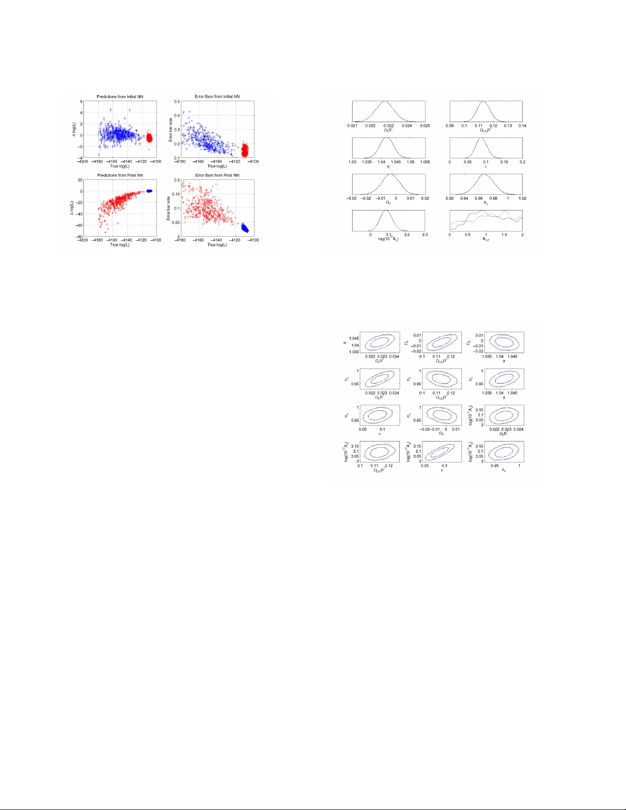
Mon. Not. R. Astron. Soc. 000 , 1–12 (2011) Printed 27 November 2024 (MN L A T E X style file v2.2) B AMBI: blind accelerated multimodal Bayesian infer ence Philip Graf f 1 ? , Farhan Feroz 1 , Michael P . Hobson 1 , and Anthony Lasenby 1 , 2 1 Astr ophysics Gr oup, Cavendish Labor atory, JJ Thomson A venue, Cambridge CB3 0HE, UK 2 Kavli Institute for Cosmology , Madingley Road, Cambridge CB3 0HA, UK 27 November 2024 ABSTRA CT In this paper , we present an algorithm for rapid Bayesian analysis that combines the benefits of nested sampling and artificial neural networks. The blind accelerated multimodal Bayesian in- ference (BAMBI) algorithm implements the M U L T I N E S T package for nested sampling as well as the training of an artificial neural netw ork (NN) to learn the lik elihood function. In the case of computationally expensi ve likelihoods, this allo ws the substitution of a much more rapid approximation in order to increase significantly the speed of the analysis. W e begin by demon- strating, with a few toy examples, the ability of a NN to learn complicated likelihood surfaces. B AMBI’ s ability to decrease running time for Bayesian inference is then demonstrated in the context of estimating cosmological parameters from W ilkinson Micr owave Anisotr opy Pr obe and other observations. W e show that v aluable speed increases are achieved in addition to obtaining NNs trained on the likelihood functions for the dif ferent model and data combi- nations. These NNs can then be used for an e ven faster follow-up analysis using the same likelihood and different priors. This is a fully general algorithm that can be applied, without any pre-processing, to other problems with computationally e xpensive lik elihood functions. Key words: methods: data analysis – methods: statistical – cosmological parameters 1 INTR ODUCTION Bayesian methods of inference are widely used in astronomy and cosmology and are g aining popularity in other fields, such as par- ticle physics. They can generally be di vided into the performance of tw o main tasks: parameter estimation and model selection. The former has traditionally been performed using Marko v chain Monte Carlo (MCMC) methods, usually based on the Metropolis-Hastings algorithm or one of its variants. These can be computationally e x- pensiv e in their exploration of the parameter space and often need to be finely tuned in order to produce accurate results. Additionally , sampling ef ficiency can be seriously af fected by multimodal distri- butions and large, curving degeneracies. The second task of model selection is further hampered by the need to calculate the Bayesian evidence accurately . The most common method of doing so is ther- modynamic inte gration, which requires se veral chains to be run, thus multiplying the computational e xpense. Fast methods of e v- idence calculation, such as assuming a Gaussian peak, clearly fail in multimodal and degenerate situations. Nested sampling (Skilling 2004) is a method of Monte Carlo sampling designed for efficient calculation of the evidence which also provides samples from the posterior distrib ution as a by-product, thus allowing parameter es- timation at no additional cost. The M U LT I N E S T algorithm (Feroz & Hobson 2008; Feroz et al. 2009a) is a generic implementation of nested sampling, e xtended to handle multimodal and degenerate distributions, and is fully parallelised. ? Email: p.graff@mrao.cam.ac.uk At each point in parameter space, Bayesian methods require the ev aluation of a ‘likelihood’ function describing the probability of obtaining the data for a giv en set of model parameters. For some cosmological and particle physics problems each such function ev aluation takes up to tens of seconds. MCMC applications may require millions of these ev aluations, making them prohibitiv ely costly . M U L T I N E S T is able to reduce the number of lik elihood function calls by an order of magnitude or more, but further gains can be achiev ed if we are able to speed up the ev aluation of the like- lihood itself. An artificial neural network (NN) is ideally suited for this task. A universal approximation theorem assures us that we can accurately and precisely approximate the likelihood with a NN of a giv en form. The training of NNs is one of the most widely studied problems in machine learning, so techniques for learning the likeli- hood function are well established. W e implement a variant of con- jugate gradient descent to find the optimum set of weights for a NN, using regularisation of the likelihood and a Hessian-free second- order approximation to improve the quality of proposed steps to- wards the best fit. The blind accelerated multimodal Bayesian inference (B AMBI) algorithm combines these two elements. After a specified number of new samples from M U L T I N E S T have been obtained, BAMBI uses these to train a network on the likelihood function. After con vergence to the optimal weights, we test that the network is able to predict likelihood values to within a specified tolerance lev el. If not, sampling continues using the original likeli- hood until enough new samples have been made for training to be done again. Once a network is trained that is sufficiently accurate, c  2011 RAS 2 Graf f, F er oz, Hobson, and Lasenby its predictions are used in place of the original likelihood function for future samples for M U L T I N E S T . Using the network reduces the likelihood ev aluation time from seconds to milliseconds, allowing M U L T I N E S T to complete the analysis much more rapidly . As a bonus, the user also obtains a network that is trained to easily and quickly provide more likelihood ev aluations near the peak if needed, or in subsequent analyses. The structure of the paper is as follows. In Section 2 we will introduce Bayesian inference and the use of nested sampling. Sec- tion 3 will then e xplain the structure of a NN and ho w our optimiser works to find the best set of weights. W e present some toy examples with B AMBI in Section 4 to demonstrate its capabilities; we apply B AMBI to cosmological parameter estimation in Section 5. In Sec- tion 6 we show the full potential speed-up from B AMBI, by using the trained NNs in a follow-up analysis. Section 7 summarises our work and presents our conclusions. 2 B A YESIAN INFERENCE AND M U L T I N E S T 2.1 Theory of Bayesian Inference Bayesian statistical methods pro vide a consistent way of estimating the probability distribution of a set of parameters Θ for a gi ven model or hypothesis H giv en a data set D . Bayes’ theorem states that Pr( Θ | D , H ) = Pr( D | Θ , H ) Pr( Θ | H ) Pr( D | H ) , (1) where Pr( Θ | D , H ) is the posterior probability distribution of the parameters and is written as P ( Θ ) , Pr( D | Θ , H ) is the likelihood and is written as L ( Θ ) , Pr( Θ | H ) is the prior distribution and is written as π ( Θ ) , and Pr( D | H ) is the Bayesian e vidence and is written as Z . The evidence is the factor required to normalise the posterior ov er Θ , Z = Z L ( Θ ) π ( Θ ) d N Θ , (2) where N is the dimensionality of the parameter space. Since the Bayesian e vidence is independent of the parameter values, Θ , it can be ignored in parameter estimation problems and the posterior inferences obtained by exploring the un–normalized posterior . Bayesian parameter estimation has achieved widespread use in many astrophysical applications. Standard Monte Carlo methods such as the Metropolis–Hastings algorithm or Hamiltonian sam- pling (see MacKay 2003) can experience problems with multi- modal likelihood distributions, as the y can get stuck in a single mode. Additionally , long and curving degeneracies are difficult for them to explore and can greatly reduce sampling efficiency . These methods often require careful tuning of proposal jump distributions and testing for con vergence can be problematic. Additionally , cal- culation of the evidence for model selection often requires running multiple chains, greatly increasing the computational cost. Nested sampling and the M ULT I N E S T algorithm implementation address these problems. 2.2 Nested Sampling Nested sampling (Skilling 2004) is a Monte Carlo method used for the computation of the evidence that can also provide posterior in- ferences. It transforms the multi-dimensional integral of Equation 2 (a) (b) Figure 1. Cartoon illustrating (a) the posterior of a two dimensional prob- lem; and (b) the transformed L ( X ) function where the prior volumes X i are associated with each likelihood L i . Originally published in Feroz & Hobson (2008). into a one-dimensional inte gral over the prior volume. This is done by defining the prior volume X as dX = π ( Θ ) d N Θ . Therefore, X ( λ ) = Z L ( Θ ) >λ π ( Θ ) d N Θ . (3) This integral extends over the region of parameter space contained within the likelihood contour L ( Θ ) = λ . The evidence integral, Equation 2, can then be written as Z = Z 1 0 L ( X ) dX , (4) where L ( X ) is the inverse of Equation 3 and is a monotonically decreasing function of X . Thus, if we ev aluate the likelihoods L i = L ( X i ) , where X i is a sequence of decreasing values, 0 < X M < · · · < X 2 < X 1 < X 0 = 1 . (5) The evidence can then be approximated numerically as a weighted sum Z = M X i =1 L i w i , (6) where the weights w i for the simple trapezium rule are giv en by w i = 1 2 ( X i − 1 − X i +1 ) . An example of a posterior in two dimen- sions and its associated function L ( X ) is sho wn in Figure 1. The fundamental operation of nested sampling begins with the initial, ‘liv e’, points being chosen at random from the entire prior volume. The lowest likelihood liv e point is removed and replaced by a ne w sample with higher likelihood. This remo val and replace- ment of liv e points continues until a stopping condition is reached (M U LT I N E S T uses a tolerance on the evidence calculation). The difficult task lies in finding a ne w sample with higher likelihood than the discarded point. As the algorithm goes up in likelihood, the prior volume that will satisfy this condition decreases until it con- tains only a very small portion of the total parameter space, making this sampling potentially very inefficient. M U LTI N E S T tackles this problem by enclosing all of the acti ve points in clusters of ellip- soids. New points can then be chosen from within these ellipsoids using a fast analytic function. Since the ellipsoids will decrease in size along with the distribution of liv e points, their surfaces in ef- fect represent likelihood contours of increasing value; the algorithm climbs up these contours seeking new points. As the clusters of el- lipsoids are not constrained to fit any particular distribution, they can easily enclose curving degeneracies and are able to separate out to allow for multimodal distributions. This separation also al- lows for the calculation of the ‘local’ evidence associated with each c  2011 RAS, MNRAS 000 , 1–12 B AMBI 3 Figure 2. A 3-layer neural network with 3 inputs, 4 hidden nodes, and 2 outputs. Image courtesy of W ikimedia Commons. mode. M U LT I N E S T has been shown to be of substantial use in as- trophysics and particle physics (see Feroz et al. 2008a,b, 2009b,c, 2010; T rotta et al. 2008; Gair et al. 2010), typically showing great improv ement in efficiency ov er traditional MCMC techniques. 3 AR TIFICIAL NEURAL NETWORKS AND WEIGHTS OPTIMISA TION Artificial neural networks are a method of computation loosely based on the structure of a brain. They consist of a group of inter- connected nodes, which process information that they receive and then pass this along to other nodes via weighted connections. W e will consider only feed-forward NN, for which the structure is di- rected, with a layer of input nodes passing information to an output layer , via zero, one, or many hidden layers in between. A network is able ‘learn’ a relationship between inputs and outputs given a set of training data and can then make predictions of the outputs for new input data. Further introduction can be found in MacKay (2003). 3.1 Network Structure A multilayer perceptron artificial neural network (NN) is the sim- plest type of network and consists of ordered layers of perceptron nodes that pass scalar values from one layer to the ne xt. The percep- tron is the simplest kind of node, and maps an input vector x ∈ < n to a scalar output f ( x ; w , θ ) via f ( x ; w , θ ) = θ + n X i =1 w i x i , (7) where { w i } and θ are the parameters of the perceptron, called the ‘weights’ and ‘bias’, respectively . W e will focus mainly on 3-layer NNs, which consist of an input layer , a hidden layer, and an output layer as shown in Figure 2. The outputs of the nodes in the hidden and output layers are giv en by the following equations: hidden layer: h j = g (1) ( f (1) j ); f (1) j = θ (1) j + X l w (1) j l x l , (8) output layer: y i = g (2) ( f (2) i ); f (2) i = θ (2) i + X j w (2) ij h j , (9) where l runs o ver input nodes, j runs ov er hidden nodes, and i runs ov er output nodes. The functions g (1) and g (2) are called activ ation functions and must be bounded, smooth, and monotonic for our purposes. W e use g (1) ( x ) = tanh( x ) and g (2) ( x ) = x ; the non- linearity of g (1) is essential to allowing the network to model non- linear functions. The weights and biases are the v alues we wish to determine in our training (described in Section 3.3). As they vary , a huge range of non-linear mappings from inputs to outputs is possible. In fact, a ‘universal approximation theorem’ (see Hornik, Stinchcombe & White 1990) states that a NN with three or more layers can ap- proximate any continuous function as long as the activation func- tion is locally bounded, piecewise continuous, and not a polynomial (hence our use of tanh , although other functions would work just as well, such as a sigmoid). By increasing the number of hidden nodes, we can achieve more accuracy at the risk of overfitting to our training data. As long as the mapping from model parameters to predicted data is continuous – and it is in many cases – the likelihood func- tion will also be continuous. This makes a NN an ideal tool for approximating the likelihood. 3.2 Choosing the Number of Hidden Layer Nodes An important choice when using a NN is the number of hidden layer nodes to use. W e consider here just the case of three-layer networks with only one hidden layer . The optimal number is a com- plex relationship between of the number of training data points, the number of inputs and outputs, and the complexity of the function to be trained. Choosing too fe w nodes will mean that the NN is unable to learn the likelihood function to sufficient accuracy . Choosing too many will increase the risk of overfitting to the training data and will also slow down the training process. As a general rule, a NN should not need more hidden nodes than the number of training data points. W e choose to use 50 or 100 nodes in the hidden layer in our examples. These choices allow the network to model the complex- ity of the likelihood surface and its functional dependency on the input parameters. The toy examples (Section 4) have fewer inputs that result in more complicated surfaces, but with simple functional relationships. The cosmological examples (Section 5) ha ve more inputs with complex relationships to generate a simple likelihood surface. In practice, it will be better to o ver -estimate the number of hidden nodes required. There are checks built in to prevent over - fitting and for computationally e xpensive likelihoods the additional training time will not be a large penalty if a usable network can be obtained earlier in the analysis. 3.3 Network T raining W e wish to use a NN to model the likelihood function giv en some model and associated data. The input nodes are the model param- eters and the single output is the value of the likelihood function at that point. The set of training data, D = { x ( k ) , t ( k ) } , is the last updInt number of points accepted by M U L T I N E S T , a parameter that is set by the user . This data is split into two groups randomly; approximately 80% is used for training the network and 20% is used as validation data to avoid ov erfitting. If training does not produce a sufficiently accurate network, M U LT I N E S T will obtain updInt / 2 ne w samples before attempting to train again. Addi- tionally , the range of log-likelihood values must be within a user- specified range or NN training will be postponed. c  2011 RAS, MNRAS 000 , 1–12 4 Graf f, F er oz, Hobson, and Lasenby 3.3.1 Overview The weights and biases we will collectively call the network pa- rameter vector a . W e can now consider the probability that a giv en set of network parameters is able to reproduce the known training data outputs – representing how well our NN model of the original likelihood reproduces the true values. This gi ves us a log-likelihood function for a , depending on a standard χ 2 error function, giv en by log( L ( a ; σ )) = − K log(2 π ) 2 − log( σ ) (10) − 1 2 K X k =1  t ( k ) − y ( x ( k ) ; a ) σ  2 , where K is the number of data points and y ( x ( k ) ; a ) is the NN’ s predicted output value for the inputs x ( k ) and network parameters a . The value of σ is a hyper-parameter of the model that describes the standard de viation (error size) of the output. Our algorithm con- siders the parameters a to be probabilistic with a log-prior distrib u- tion giv en by log( S ( a ; α )) = − α 2 X i a 2 i . (11) α is a hyper-parameter of the model, called the ‘regularisation con- stant’, that gives the relative influence of the prior and the likeli- hood. The posterior probability of a set of NN parameters is thus Pr( a ; α, σ ) ∝ L ( a ; σ ) × S ( a ; α ) . (12) B AMBI’ s network training begins by setting random values for the weights, sampled from a normal distribution with zero mean. The initial value of σ is set by the user and can be set on ei- ther the true log-likelihood values themselves or on their whitened values (whitening in volv es performing a linear transform such that the training data values have a mean of zero and standard de via- tion of one). The only difference between these two settings is the magnitude of the error used. The algorithm then calculates a large initial estimate for α , α = |∇ log( L ) | √ M r , (13) where M is the total number of weights and biases (NN parame- ters) and r is a rate set by the user ( 0 < r 6 1 , default r = 0 . 1 ) that defines the size of the ‘confidence re gion’ for the gradient. This formula for α sets larger regularisation (‘damping’) when the mag- nitude of the gradient of the likelihood is lar ger . This relates the amount of “smoothing” required to the steepness of the function being smoothed. The rate factor in the denominator allo ws us to increase the damping for smaller confidence regions on the value of the gradient. This results in smaller , more conserv ative steps that are more likely to result in an increase in the function v alue. B AMBI then uses conjug ate gradients to calculate a step, ∆ a , that should be taken (see Section 3.3.2). Follo wing a step, adjust- ments to α and σ may be made before another step is calculated. The methods for calculating the initial α value and then determin- ing subsequent adjustments of α and/or σ are as developed for the M E M S YS software package, described in Gull & Skilling (1999). 3.3.2 F inding the next step In order to find the most efficient path to an optimal set of parame- ters, we perform conjugate gradients using second-order deri vati ve information. Newton’ s method gives the second-order approxima- tion of a function, f ( a + ∆ a ) ≈ f ( a ) + ( ∇ f ( a )) T ∆ a + 1 2 (∆ a ) T B ∆ a , (14) where B is the Hessian matrix of second derivati ves of f at a . In this approximation, the maximum of f will occur when ∇ f ( a + ∆ a ) ≈ ∇ f ( a ) + B ∆ a = 0 . (15) Solving this for ∆ a giv es us ∆ a = − B − 1 ∇ f ( a ) . (16) Iterating this procedure will bring us ev entually to the global max- imum value of f . For our purposes, the function f is the log- posterior distrib ution and hence Equation (14) is a Gaussian ap- proximation to the posterior . The Hessian of the log-posterior is the regularised (‘damped’) Hessian of the log-likelihood function, where the prior – whose magnitude is set by α – provides the reg- ularisation. If we define the Hessian matrix of the log-likelihood as H , then B = H + α I ( I being the identity matrix). Using the second-order information provided by the Hessian allows for more efficient steps to be made, since curv ature infor- mation can extend step sizes in directions where the gradient varies less and shorten where it is varying more. Additionally , using the Hessian of the log-posterior instead of the log-likelihood adds the regularisation of the prior, which can help to prev ent getting stuck in a local maximum by smoothing out the function being e xplored. It also aids in reducing the ‘region of confidence’ for the gradient information which will make it less likely that a step results in a worse set of parameters. Giv en the form of the log-likelihood, Equation (10), is a sum of squares (plus a constant), we can also save computational ex- pense by utilising the Gauss-Newton approximation of its Hessian, giv en by H ij = − K X k =1  ∂ r k ∂ a i ∂ r k ∂ a j + r k ∂ 2 r k ∂ a i ∂ a j  (17) ≈ − K X k =1  ∂ r k ∂ a i ∂ r k ∂ a j  , where r k = t ( k ) − y ( x ( k ) ; a ) σ . (18) The drawback of using second-order information is that cal- culation of the Hessian is computationally expensiv e and requires large storage, especially so in many dimensions as we will en- counter for more complex networks. In general, the Hessian is not guaranteed to be positive semi-definite and so may not be in- vertible; howe ver , the Gauss-Netwon approximation does have this guarantee. In version of the very large matrix will still be computa- tionally expensi ve. As noted in Martens (2010) howe ver , we only need products of the Hessian with a v ector to compute the solution, nev er actually the full Hessian itself. T o calculate these approxi- mate Hessian-vector products, we use a fast approximate method giv en in Schraudolph (2002) and Pearlmutter (1994). Combining all of these methods makes second-order information practical to use. 3.3.3 Con verg ence Follo wing each step, the posterior , likelihood, and correlation val- ues are calculated for the training data and the validation data that c  2011 RAS, MNRAS 000 , 1–12 B AMBI 5 was not used in training (calculating the steps). Conv ergence to a best-fit set of parameters is determined by maximising the poste- rior , likelihood, or correlation of the validation data, as chosen by the user . This prev ents ov erfitting as it pro vides a check that the network is still valid on points not in the training set. W e use the correlation as the def ault function to maximise as it does not in- clude the model hyper-parameters in its calculation. 3.4 When to Use the T rained Network The optimal network possible with a gi ven set of training data may not be able to predict likelihood values accurately enough, so an ad- ditional criterion is placed on when to use the trained network. This requirement is that the standard de viation of the dif ference between predicted and true log-lik elihood values is less than a user-specified tolerance. When the trained network does not pass this test, then B AMBI will continue using the original log-likelihood function to obtain updInt / 2 new samples to generate a new training data set of the last updInt accepted samples. Network training will then resume, be ginning with the weights that it had found as optimal for the previous data set. Since samples are generated from nested con- tours and each new data set contains half of the previous one, the sav ed network will already be able to produce reasonable predic- tions on this new data; resuming therefore enables us to save time as fewer steps will be required to reach the ne w optimum weights. Once a NN is in use in place of the original log-likelihood function, checks are made to ensure that the network is main- taining its accuracy . If the network makes a prediction outside of [ min ( training ) − σ, max ( training ) + σ ] , then that v alue is discarded and the original log-likelihood function is used for that point. Ad- ditionally , the central 95 th percentile of the output log-likelihood values from the training data used is calculated and if the network is making predictions mostly outside of this range then it will be re- trained. T o re-train the network, BAMBI first substitutes the origi- nal log-likelihood function back in and g athers the required number of new samples from M U LT I N E S T . Training then commences, re- suming from the previously saved network. These criteria ensure that the network is not trusted too much when making predictions beyond the limits of the data it was trained on, as we cannot be sure that such predictions are accurate. 4 B AMBI TO Y EXAMPLES In order to demonstrate the ability of BAMBI to learn and accu- rately explore multimodal and degenerate likelihood surfaces, we first tested the algorithm on a few toy examples. The eggbox like- lihood has many separate peaks of equal likelihood, meaning that the network must be able to make predictions across many differ- ent areas of the prior . The Gaussian shells likelihood presents the problem of making predictions in a v ery narrow and curving region. Lastly , the Rosenbrock function gives a long, curving degenerac y that can also be extended to higher dimensions. They all require high accuracy and precision in order to reproduce the posterior truthfully and each presents unique challenges to the NN in learn- ing the likelihood. It is important to note that running BAMBI on these problems required more time than the straightforward anal- ysis; this was as expected since the actual likelihood functions are simple analytic functions that do not require much computational expense. Figure 3. The eggbox log-lik elihood surface, given by Equation (19). Method log( Z ) Analytical 235 . 88 M U L T I N ES T 235 . 859 ± 0 . 039 B AMBI 235 . 901 ± 0 . 039 T able 1. The log-evidence values of the eggbox likelihood as found analyt- ically and with M U LTI N E S T and BAMBI. 4.1 Eggbox This is a standard example of a very multimodal likelihood distri- bution in two dimensions. It has many peaks of equal value, so the network must be able to take samples from separated regions of the prior and make accurate predictions in all peaks. The eggbox likelihood (Feroz et al. 2009a) is gi ven by L ( x, y ) = exp h  2 + cos( x 2 ) cos( y 2 )  5 i , (19) where we tak e a uniform prior U (0 , 10 π ) for both x and y . The structure of the surface can be seen in Figure 3. W e ran the eggbox example in both M U LTI N E S T and B AMBI, both using 4000 live points. For BAMBI, we used 4000 samples for training a network with 50 hidden nodes. In T able 1 we report the evidences recovered by both methods as well as the true value obtained analytically from Equation (19). Both methods return ev- idences that agree with the analytically determined value to within the giv en error bounds. Figure 4 compares the posterior probabil- ity distrib utions returned by the two algorithms via the distribu- tion of lo west-likelihood points removed at successi ve iterations by M U L T I N E S T . W e can see that they are identical distributions; there- fore, we can say that the use of the NN did not reduce the quality of the results either for parameter estimation or model selection. During the BAMBI analysis 51 . 3% of the log-likelihood function ev aluations were done using the NN; if this were a more compu- tationally expensi ve function, significant speed g ains would have been realised. 4.2 Gaussian Shells The Gaussian shells likelihood function has low values over most of the prior , e xcept for thin circular shells that ha ve Gaussian cross- sections. W e use two separate Gaussian shells of equal magnitude so that this is also a mutlimodal inference problem. Therefore, our c  2011 RAS, MNRAS 000 , 1–12 6 Graf f, F er oz, Hobson, and Lasenby (a) (b) Figure 4. Points of lo west likelihood of the e ggbox likelihood from succes- siv e iterations as given by (a) M U L T I N E ST and (b) BAMBI. Figure 5. The Gaussian shell likelihood surface, given by Equations (20) and (21). Gaussian shells likelihood is L ( x ) = circ ( x ; c 1 , r 1 , w 1 ) + circ ( x ; c 2 , r 2 , w 2 ) , (20) where each shell is defined by circ ( x ; c , r, w ) = 1 √ 2 π w 2 exp  − ( | x − c | − r ) 2 2 w 2  . (21) This is shown in Figure 5. As with the eggbox problem, we analysed the Gaussian shells likelihood with both M U LT I N E S T and BAMBI using uniform pri- ors U ( − 6 , 6) on both dimensions of x . M U LT I N E S T sampled with 1000 liv e points and B AMBI used 2000 samples for training a net- work with 100 hidden nodes. In T able 2 we report the e vidences re- cov ered by both methods as well as the true value obtained analyti- cally from Equations (20) and (21). The evidences are both consis- tent with the true value. Figure 6 compares the posterior probability distributions returned by the two algorithms (in the same manner as with the e ggbox example). Again, we see that the distrib ution of re- turned values is nearly identical when using the NN, which BAMBI used for 18 . 2% of its log-likelihood function ev aluations. This is a significant fraction, especially since they are all at the end of the analysis when exploring the peaks of the distrib ution. 4.3 Rosenbrock function The Rosenbrock function is a standard e xample used for testing op- timization as it presents a long, curved degenerac y through all di- mensions. F or our NN training, it presents the difficulty of learning the lik elihood function over a large, curving region of the prior . W e Method log( Z ) Analytical − 1 . 75 M U L T I N ES T − 1 . 768 ± 0 . 052 B AMBI − 1 . 757 ± 0 . 052 T able 2. The log-evidence values of the Gaussian shell likelihood as found analytically and with M U LTI N E S T and BAMBI. (a) (b) Figure 6. Points of lowest likelihood of the Gaussian shell likelihood from successiv e iterations as given by (a) M U L T I N E ST and (b) BAMBI. use the Rosenbrock function to define the negativ e log-likelihood, so the likelihood function is gi ven in N dimensions by L ( x ) = exp ( − N − 1 X i =1  (1 − x i ) 2 + 100( x i +1 − x 2 i ) 2  ) . (22) Figure 7 shows ho w this appears for N = 2 . W e set uniform priors of U ( − 5 , 5) in all dimensions and per- formed analysis with both M U LT I N E S T and BAMBI with N = 2 and N = 10 . For N = 2 , M U L T I N E S T sampled with 2000 liv e points and BAMBI used 2000 samples for training a NN with 50 hidden-layer nodes. W ith N = 10 , we used 2000 liv e points, 6000 samples for network training, and 50 hidden nodes. T able 3 giv es the calculated e vidences values returned by both algorithms as well as the analytically calculated v alues from Equation (22) (there does not exist an analytical solution for the 10D case so this is not in- cluded). Figure 8 compares the posterior probability distributions returned by the two algorithms for N = 2 . For N = 10 , we show in Figure 9 comparisons of the marginalised two-dimensional pos- terior distributions for 12 variable pairs. W e see that M U L T I N E S T and BAMBI return nearly identical posterior distributions as well Figure 7. The Rosenbrock log-likelihood surface given by Equation (22) with N = 2 . c  2011 RAS, MNRAS 000 , 1–12 B AMBI 7 Method log( Z ) Analytical 2D − 5 . 804 M U L T I N ES T 2D − 5 . 799 ± 0 . 049 B AMBI 2D − 5 . 757 ± 0 . 049 M U L T I N ES T 10D − 41 . 54 ± 0 . 13 B AMBI 10D − 41 . 53 ± 0 . 13 T able 3. The log-evidence values of the Rosenbrock likelihood as found analytically and with M U LTI N E S T and BAMBI. (a) (b) Figure 8. Points of lowest likelihood of the Rosenbrock lik elihood for N = 2 from successive iterations as gi ven by (a) M U L T I N E ST and (b) B AMBI. as consistent estimates of the evidence. For N = 2 and N = 10 , B AMBI was able to use a NN for 64 . 7% and 30 . 5% of its log- likelihood e valuations respecti vely . Even when factoring in time required to train the NN this would ha ve resulted in large decreases in running time for a more computationally e xpensive likelihood function. 5 COSMOLOGICAL P ARAMETER ESTIMA TION WITH B AMBI While likelihood functions resembling our previous toy examples do exist in real physical models, we would also like to demonstrate the usefulness of B AMBI on simpler likelihood surfaces where the time of ev aluation is the critical limiting factor . One such example Figure 9. Mar ginalised 2D posteriors for the Rosenbrock function with N = 10 . The 12 most correlated pairs are shown. M U LTI N E S T is in solid black, B AMBI in dashed blue. Inner and outer contours represent 68% and 95% confidence levels, respecti vely . Parameter Min Max Ω b h 2 0 . 018 0 . 032 Ω DM h 2 0 . 04 0 . 16 θ 0 . 98 1 . 1 τ 0 . 01 0 . 5 Ω K − 0 . 1 0 . 1 n s 0 . 8 1 . 2 log[10 10 A s ] 2 . 7 4 A S Z 0 2 T able 4. The cosmological parameters and their minimum and maximum values. Uniform priors were used on all variables. Ω K was set to 0 for the flat model. in astrophysics is that of cosmological parameter estimation and model selection. W e implement B AMBI within the standard C O S M O M C code (Lewis & Bridle 2002), which by default uses MCMC sam- pling. This allows us to compare the performance of B AMBI with other methods, such as M U L T I N E S T (Feroz et al. 2009a), C O S - M O N E T (Auld et al. 2007, 2008), I N T E RP M C (Bouland et al. 2011), PICO (Fendt & W andelt 2006), and others. In this paper , we will only report performances of B AMBI and M U L T I N E S T , but these can be compared with reported performance from the other methods. Bayesian parameter estimation in cosmology requires evalua- tion of theoretical temperature and polarisation CMB power spec- tra ( C l values) using codes such as CAMB (Le wis et al. 2000). These ev aluations can take on the order of tens of seconds depend- ing on the cosmological model. The C l spectra are then compared to WMAP and other observ ations for the likelihood function. Con- sidering that thousands of these e valuations will be required, this is a computationally expensi ve step and a limiting factor in the speed of any Bayesian analysis. W ith BAMBI, we use samples to train a NN on the combined likelihood function which will allow us to forgo ev aluating the full power spectra. This has the benefit of not requiring a pre-computed sample of points as in C O S M O N E T and PICO, which is particularly important when including new param- eters or new physics in the model. In these cases we will not know in adv ance where the peak of the likelihood will be and it is around this location that the most samples would be needed for accurate results. The set of cosmological parameters that we use as variables and their prior ranges is gi ven in T able 4; the parameters have their usual meanings in cosmology (see Larson et al. 2011, table 1). The prior probability distrib utions are uniform ov er the ranges giv en. A non-flat cosmological model incorporates all of these parameters, while we set Ω K = 0 for a flat model. W e use w = − 1 in both cases. The flat model thus represents the standard Λ CDM cosmol- ogy . W e use two dif ferent data sets for analysis: ( 1 ) CMB obser- vations alone and ( 2 ) CMB observations plus Hubble Space T ele- scope constraints on H 0 , large-scale structure constraints from the luminous red galaxy subset of the SDSS and the 2dF survey , and supernov ae Ia data. The CMB dataset consists of WMAP sev en- year data (Larson et al. 2011) and higher resolution observations from the ACB AR, CBI, and BOOMERanG experiments. The C O S - M O M C website (see Le wis & Bridle 2002) provides full references for the most recent sources of these data. Analyses with M U LT I N E S T and B AMBI were run on all four combinations of models and data sets. M U L T I N E S T sampled with 1000 liv e points and an efficiency of 0 . 5 , both on its own and within B AMBI; BAMBI used 2000 samples for training a NN on the like- c  2011 RAS, MNRAS 000 , 1–12 8 Graf f, F er oz, Hobson, and Lasenby Algorithm Model Data Set log( Z ) M U L T I N ES T Λ CDM CMB only − 3754 . 58 ± 0 . 12 B AMBI Λ CDM CMB only − 3754 . 57 ± 0 . 12 M U L T I N ES T Λ CDM all − 4124 . 40 ± 0 . 12 B AMBI Λ CDM all − 4124 . 11 ± 0 . 12 M U L T I N ES T Λ CDM +Ω K CMB only − 3755 . 26 ± 0 . 12 B AMBI Λ CDM +Ω K CMB only − 3755 . 57 ± 0 . 12 M U L T I N ES T Λ CDM +Ω K all − 4126 . 54 ± 0 . 13 B AMBI Λ CDM +Ω K all − 4126 . 35 ± 0 . 13 T able 5. Evidences calculated by M U L T I N ES T and BAMBI for the flat ( Λ CDM) and non-flat ( Λ CDM +Ω K ) models using the CMB-only and complete data sets. The two algorithms are in close agreement in all cases. Figure 10. Marginalised 1D posteriors for the non-flat model ( Λ CDM +Ω K ) using only CMB data. M U L T I N E ST is in solid black, B AMBI in dashed blue. lihood, with 50 hidden-layer nodes for both the flat model and non- flat model. T able 5 reports the recovered evidences from the two algorithms for both models and both data sets. It can be seen that the two algorithms report equiv alent values to within statistical er- ror for all four combinations. In Figures 10 and 11 we sho w the recov ered one- and two-dimensional marginalised posterior proba- bility distributions for the non-flat model using the CMB-only data set. Figures 12 and 13 show the same for the non-flat model us- ing the complete data set. W e see v ery close agreement between M U L T I N E S T (in solid black) and B AMBI (in dashed blue) across all parameters. The only exception is A S Z since it is unconstrained by these models and data and is thus subject to large amounts of variation in sampling. The posterior probability distrib utions for the flat model with either data set are extremely similar to those of the non-flat flodel with setting Ω K = 0 , as expected, so we do not show them here. A by-product of running B AMBI is that we now hav e a net- work that is trained to predict lik elihood v alues near the peak of the distribution. T o see how accurate this network is, in Figure 14 we plot the error in the prediction ( ∆ log ( L ) = log( L predicted ) − log( L true ) ) versus the true log-likelihood value for the different sets of training and v alidation points that were used. What we sho w are results for netw orks that were trained to suf ficient accurac y in order to be used for making lik elihood predictions; this results in tw o net- works for each case sho wn. W e can see that although the flat model Figure 11. Marginalised 2D posteriors for the non-flat model ( Λ CDM +Ω K ) using only CMB data. The 12 most correlated pairs are shown. M U L T I N ES T is in solid black, BAMBI in dashed blue. Inner and outer contours represent 68% and 95% confidence levels, respecti vely . Figure 12. Marginalised 1D posteriors for the non-flat model ( Λ CDM +Ω K ) using the complete data set. M U L T I N E ST is in solid black, B AMBI in dashed blue. used the same number of hidden-layer nodes, the simpler physical model allowed for smaller error in the likelihood predictions. Both final networks (one for each model) are significantly more accu- rate than the specified tolerance of a maximum standard deviation on the error of 0 . 5 . In fact, for the flat model, all b ut one of the 2000 points ha ve an error of less than 0 . 06 log-units. The two net- works trained in each case overlap in the range of log-likelihood values on which they trained. The first network, although trained to lower accuracy , is valid over a much lar ger range of log-likelihoods. The accuracy of each network increases with increasing true log- likelihood and the second netw ork, trained on higher log-likelihood values, is significantly more accurate than the first. The final comparison, and perhaps the most important, is the running time required. The analyses were run using MPI paral- lelisation on 48 processors. W e recorded the time required for the complete analysis, not including any data initialisation prior to ini- tial sampling. W e then divide this time by the number of likeli- hood ev aluations performed to obtain an average time per likeli- hood ( t wall clock, sec × N CPUs / N log( L ) evals ). Therefore, time required to train the NN is still counted as a penalty factor . If a NN takes c  2011 RAS, MNRAS 000 , 1–12 B AMBI 9 Figure 13. Marginalised 2D posteriors for the non-flat model ( Λ CDM +Ω K ) using the complete data set. The 12 most correlated pairs are shown. M U LTI N E S T is in solid black, BAMBI in dashed blue. Inner and outer contours represent 68% and 95% confidence lev els, respectiv ely . Figure 14. The error in the predicted likelihood ( ∆ log( L ) = log( L predicted ) − log( L true ) ) for the BAMBI networks trained on the flat (top row) and non-flat (bottom row) models using the complete data set. The left column represents predictions from the first NN trained to suffi- cient accuracy; the right column are results from the second, and final, NN trained in each case. The flat and non-flat models both used 50 hidden-layer nodes. more time to train, this will hurt the average time, but obtaining a usable NN sooner and with fewer training calls will give a better time since more likelihoods will be ev aluated by the NN. The re- sulting average times per likelihood and speed increases are giv en in T able 6. Although the speed increases appear modest, one must remember that these include time taken to train the NNs, during which no likelihoods were evaluated. This can be seen in that al- though 30 – 40% of likelihoods are e valuated with a NN, as reported in T able 7, we do not obtain the full equiv alent speed increase. W e are still able to obtain a significant decrease in running time while adding in the bonus of ha ving a NN trained on the likelihood func- tion. Model Data set M U LTI N E S T B AMBI Speed t L (s) t L (s) factor Λ CDM CMB only 2 . 394 1 . 902 1 . 26 Λ CDM all 3 . 323 2 . 472 1 . 34 Λ CDM +Ω K CMB only 12 . 744 9 . 006 1 . 42 Λ CDM +Ω K all 12 . 629 10 . 651 1 . 19 T able 6. Time per lik elihood evaluation, f actor of speed increase from M U L T I N ES T to BAMBI ( t MN /t BAMBI ). Model Data set % log ( L ) Equiv alent Actual with NN speed factor speed factor Λ CDM CMB only 40 . 5 1 . 68 1 . 26 Λ CDM all 40 . 2 1 . 67 1 . 34 Λ CDM +Ω K CMB only 34 . 2 1 . 52 1 . 42 Λ CDM +Ω K all 30 . 0 1 . 43 1 . 19 T able 7. Percentage of likelihood ev aluations performed with a NN, equiv- alent speed factor , and actual factor of speed increase. 6 USING TRAINED NETWORKS FOR FOLLO W-UP IN B AMBI A major benefit of BAMBI is that following an initial run the user is provided with a trained NN, or multiple ones, that model the log-likelihood function. These can be used in a subsequent analysis with different priors to obtain much faster results. This is a com- parable analysis to that of C OS M O N E T (Auld et al. 2007, 2008), except that the NNs here are a product of an initial Bayesian anal- ysis where the peak of the distribution was not previously known. No prior knowledge of the structure of the likelihood surface was used to generate the networks that are no w able to be re-used. When multiple NNs are trained and used in the initial BAMBI analysis, we must determine which network’ s prediction to use in the follo w-up. The approximate error of uncertainty of a NN’ s pre- diction of the value y ( x ; a ) ( x denoting input parameters, a NN weights and biases as before) that models the log-likelihood func- tion is giv en by MacKay (1995) as σ 2 = σ 2 pred + σ 2 ν , (23) where σ 2 pred = g T B − 1 g (24) and σ 2 ν is the variance of the noise on the output from the network training. In Equation (24), B is the Hessian of the log-posterior as before, and g is the gradient of the NN’ s prediction with respect to the weights about their maximum posterior values, g = ∂ y ( x ; a ) ∂ a | x , a MP . (25) This uncertainty of the prediction is calculated for each training and validation data point used in the initial training of the NN for each sav ed NN. The threshold for accepting a predicted point from a network is then set to be 1 . 2 times the maximum uncertainty found. A log-likelihood is calculated by first making a prediction with the final NN to be trained and sa ved and then calculating the er- ror for this prediction. If the error, σ pred , is greater than that NN’ s threshold, then we consider the previous trained NN. W e again cal- culate the predicted log-likelihood v alue and error to compare with its threshold. This continues to the first NN sa ved until a NN makes a sufficiently confident prediction. If no NNs can make a confident c  2011 RAS, MNRAS 000 , 1–12 10 Graf f, F er oz, Hobson, and Lasenby Figure 15. Predictions with uncertainty error bars for NNs saved by B AMBI when analysing the non-flat model using the complete data set. The left-hand side shows predictions with errors for the two NNs on their o wn and the other’ s validation data sets. Each network’ s own points are in blue +s, the other NN’ s points are in red crosses. Many error bars are too small to be seen. The right-hand side, using the same colour and label scheme, shows the magnitudes of the error bars from each NN on the predictions. enough prediction, then we set log( L ) = −∞ . This is justified because the NNs are trained to predict values in the highest like- lihood regions of parameter space and if a set of parameters lies outside their collectiv e region of v alidity , then it must not be within the region of highest likelihoods. T o demonstrate the speed-up potential of using the NNs, we first ran an analysis of the cosmological parameter estimation us- ing both models and both data sets. This time, howev er, we set the tolerance of the NNs to 1 . 0 instead of 0 . 5 , so that they would be valid over a larger range of log-likelihoods and pass the accuracy criterion sooner . Each analysis produced two trained NNs. W e then repeated each of the four analyses, but set the prior ranges to be uni- form over the region defined by x max (log( L )) ± 4 σ , where σ is the vector of standard deviations of the marginalised one-dimensional posterior probabilities. In Figure 15 we show predictions from the two trained NNs on the two sets of validation data points in the case of the non-flat model using the complete data set. In the left-hand column, we can see that the first NN trained is able to make reasonable predictions on its own v alidation data as well as on the second set of points, in red crosses, from the second NN’ s validation data. The final NN is able to make more precise predictions on its own data set than the initial NN, but is unable to make accurate predictions on the first NN’ s data points. The right-hand column shows the error bar sizes for each of the points shown. For both NNs, the errors decrease with increasing log-likelihood. The final NN has significantly lower un- certainty on predictions for its own validation data, which enables us to set the threshold for when we can trust its prediction. The cases for the other three sets of cosmological models and data sets are very similar to this one. This demonstrates the need to use the uncertainty error measurement in determining which NN predic- tion to use, if any . Always using the final NN would produce poor predictions away from the peak and the initial NN does not have sufficient precision near the peak to properly measure the best-fit cosmological parameters. But by choosing which NN’ s prediction to accept, as we hav e shown, we can quickly and accurately repro- duce the likelihood surface for sampling. Furthermore, if one were interested only in performing a re-analysis about the peak, then one Figure 16. Marginalised 1D posteriors for the non-flat model ( Λ CDM +Ω K ) using the complete data set. BAMBI’ s initial run is in solid black, the follow-up analysis in dashed blue. Figure 17. Marginalised 2D posteriors for the non-flat model ( Λ CDM +Ω K ) using the complete data set. The 12 most correlated pairs are sho wn. B AMBI’ s initial run is in solid black, the follow-up analysis in dashed blue. Inner and outer contours represent 68% and 95% confidence lev els, respectively . could use just the final NN, thereby omitting the calculational over - head associated with choosing the appropriate network. For this same case, we plot the one- and two-dimensional marginalised posterior probabilities in Figures 16 and 17, respec- tiv ely . Although the priors do not cover exactly the same ranges, we expect very similar posterior distributions since the priors are sufficiently wide as to encompass nearly all of the posterior proba- bility . W e see this very close agreement in all cases. Calculating the uncertainty error requires calculating approx- imate in verse Hessian-vector products which slow do wn the pro- cess. W e sacrifice a large f actor of speed increase in order to main- tain the robustness of our predictions. Using the same method as before, we computed the time per likelihood calculation for the ini- tial BAMBI run as well as the follo w up; these are compared in T able 8. W e can see that in addition to the initial speed-up obtained with B AMBI, this follow-up analysis obtains an even larger speed- up in time per likelihood calculation. This speed-up is especially large for the non-flat model, where CAMB takes longer to com- pute the CMB spectra. The speed factor also increases when using c  2011 RAS, MNRAS 000 , 1–12 B AMBI 11 Model Data set Initial Follo w-up Speed t L (s) t L (s) factor Λ CDM CMB only 1 . 635 0 . 393 4 . 16 Λ CDM all 2 . 356 0 . 449 5 . 25 Λ CDM +Ω K CMB only 9 . 520 0 . 341 27 . 9 Λ CDM +Ω K all 8 . 640 0 . 170 50 . 8 T able 8. Time per lik elihood evaluation, f actor of speed increase from B AMBI’s initial run to a follo w-up analysis. the complete data set, as the original likelihood calculation takes longer than for the CMB-only data set; NN predictions take equal time regardless of the data set. One possible way to avoid the computational cost of com- puting error bars on the predictions is that suggested by MacKay (1995). One can take the NN training data and add Gaussian noise and train a new NN, using the old weights as a starting point. Per- forming many realisations of this will quickly provide multiple NNs whose a verage prediction will be a good fit to the original data and whose variance from this mean will measure the error in the prediction. This will reduce the time needed to compute an er- ror bar since multiple NN predictions are faster than a single in- verse Hessian-vector product. In vestigation of this technique will be explored in a future work. 7 SUMMAR Y AND CONCLUSIONS W e have introduced and demonstrated a new algorithm for rapid Bayesian data analysis. The Blind Accelerated Multimodal Bayesian Inference algorithm combines the sampling efficiency of M U L T I N E S T with the predictive power of artificial neural netw orks to reduce significantly the running time for computationally e xpen- siv e problems. The first applications we demonstrated are toy examples that demonstrate the ability of the NN to learn complicated likelihood surfaces and produce accurate evidences and posterior probability distributions. The eggbox, Gaussian shells, and Rosenbrock func- tions each present difficulties for Monte Carlo sampling as well as for the training of a NN. With the use of enough hidden-layer nodes and training points, we have demonstrated that a NN can learn to accurately predict log-likelihood function v alues. W e then apply B AMBI to the problem of cosmological pa- rameter estimation and model selection. W e performed this using flat and non-flat cosmological models and incorporating only CMB data and using a more e xtensive data set. In all cases, the NN is able to learn the likelihood function to sufficient accuracy after train- ing on early nested samples and then predict values thereafter . By calculating a significant fraction of the likelihood values with the NN instead of the full function, we are able to reduce the running time by a factor of 1 . 19 to 1 . 42 . This is in comparison to use of M U L T I N E S T only , which already provides significant speed-ups in comparison to traditional MCMC methods (see Feroz et al. 2009a). Through all of these examples we hav e shown the capability of B AMBI to increase the speed at which Bayesian inference can be done. This is a fully general method and one need only change the settings for M U LT I N E S T and the network training in order to apply it to different likelihood functions. For computationally ex- pensiv e likelihood functions, the network training takes less time than is required to sample enough training points and sampling a point using the netw ork is extremely rapid as it is a simple analytic function. Therefore, the main computational expense of B AMBI is calculating training points while the sampling ev olves until the net- work is able to reproduce the likelihood accurately enough. W ith the trained NN, we can no w perform additional analyses using the same likelihood function but different priors and save large amounts of time in sampling points with the original likelihood and in training a NN. F ollow-up analyses using already trained NNs provides much larger speed increases, with factors of 4 to 50 ob- tained for cosmological parameter estimation relative to BAMBI speeds. The limiting factor in these runs is the calculation of the error of predictions, which is a flat cost based on the size of the NN and data set, regardless of the original lik elihood function. The NNs trained by BAMBI for cosmology cover a larger range of log-lik elihoods than the one trained for C O S M O N E T . This allows us to use a wider range of priors for subsequent analysis and not be limited to the four-sigma region around the maximum like- lihood point. By setting the tolerance for B AMBI’ s NNs to a larger value, fewer NNs with larger likelihood ranges can be trained, al- beit with larger errors on the predictions. Allowing for larger priors requires us to test the validity of our NNs’ approximations, which ends up slowing the o verall analysis. Since B AMBI uses a NN to calculate the likelihood at later times in the analysis where we typically also suffer from lo wer sampling efficiency (harder to find a new point with higher like- lihood than most recent point removed), we are more easily able to implement Hamiltonian Monte Carlo (Betancourt 2010) for find- ing a proposed sample. This method uses gradient information to make better proposals for the next point that should be ‘sampled’. Calculating the gradient is usually a difficult task, but with the NN approximation they are very fast and simple. This improvement will be in vestigated in future work. As larger data sets and more complicated models are used in cosmology , particle physics, and other fields, the computational cost of Bayesian inference will increase. The BAMBI algorithm can, without any pre-processing, significantly reduce the required running time for these inference problems. In addition to provid- ing accurate posterior probability distrib utions and evidence calcu- lations, the user also obtains a NN trained to produce likelihood values near the peak(s) of the distribution that can be used in ev en more rapid follow-up analysis. A CKNO WLEDGMENTS PG is funded by the Gates Cambridge T rust and the Cambridge Philosophical Society; FF is supported by a T rinity Hall Colle ge re- search fellowship. The authors would like to thank Michael Bridges for useful discussions, Jonathan Zwart for inspiration in naming the algorithm, and Natallia Karpenko for helping to edit the paper . The colour scheme for Figures 3, 5, and 7 was adapted to MA T - LAB from Green (2011). This work was performed on COSMOS VIII, an SGI Altix UV1000 supercomputer , funded by SGI/Intel, HEFCE and PP ARC and the authors thank Andrey Kaliazin for assistance. The w ork also utilised the Darwin Supercomputer of the Uni versity of Cambridge High Performance Computing Ser- vice ( http://www.hpc.cam.ac.uk/ ), provided by Dell Inc. using Strategic Research Infrastructure Funding from the Higher Education Funding Council for England and the authors w ould like to thank Dr . Stuart Rankin for computational assistance. c  2011 RAS, MNRAS 000 , 1–12 12 Graf f, F er oz, Hobson, and Lasenby REFERENCES Auld T , Bridges M, Hobson M P & Gull S F , 2007, MNRAS, 376, L11, arXiv:astro-ph/0608174 Auld T , Bridges M & Hobson M P , 2008, MNRAS, 387, 1575, arXiv:astro-ph/0703445 Betancourt M, 2011, in Mohammad-Djafari A., Bercher J.-F ., Bessi ´ ere P ., eds, AIP Conf. Proc. V ol. 1305, Nested Sampling with Constrained Hamiltonian Monte Carlo. Am. Inst. Phys., New Y ork, p. 165, arXi v:1005.0157 [gr-qc] Bouland A, Easther R & Rosenfeld K, 2011, J. Cosmol. Astropart. Phys., 5, 016, arXi v:1012.5299 [astro-ph.CO] Fendt W A & W andelt B D, 2006, ApJ, 654, 2, arXiv:astro- ph/0606709 Feroz F & Hobson M P , 2008, MNRAS, 384, 449, [astro-ph] Feroz F , Allanach B C, Hobson M P , Abdus Salam S S, Trotta R & W eber A M, 2008a, J. High Energy Phys., 10, 64, arXiv:0807.4512 [hep-ph] Feroz F , Marshall P J & Hobson M P , 2008b, pre-print arXiv:0810.0781 [astro-ph] Feroz F , Hobson M P , & Bridges M, 2009a, MNRAS, 398, 1601, arXiv:0809.3437 [astro-ph] Feroz F , Hobson M P , Zwart J T L, Saunders R D E & Grainge K J B, 2009b, MNRAS, 398, 2049, arXiv:0811.1199 [astro-ph] Feroz F , Gair J, Hobson M P & Porter E K, 2009c, CQG, 26, 215003, arXiv:0904.1544 [gr -qc] Feroz F , Gair J, Graf f P , Hobson M P & Lasenby A, 2010, Classical Quantum Gravity , 27, 075010, arXiv:0911.0288 [gr -qc] Gair J, Feroz F , Babak S, Graff P , Hobson M P , Petiteau A & Porter E K, 2010, J. Phys.: Conf. Ser ., 228, 012010 Green D A, 2011, Bull. Astron. Soc. India, 39, 289, arXiv:1108.5083 [astro-ph.IM] Gull S F & Skilling J, 1999, Quantified Maximum En- tropy: MemSys 5 Users’ Manual. Maximum Entropy Data Consultants Ltd. Bury St. Edmunds, Suffolk, UK. http://www.maxent.co.uk/ Hornik K, Stinchcombe M & White H, 1990, Neural Networks, 3, 359 Larson D et al., 2011, ApJS, 192, 16, arXiv:1001.4635 [astro- ph.CO] Lewis A & Bridle S, 2002, Phys. Rev . D, 66, 103511, arXiv:astro- ph/0205436. http://cosmologist.info/cosmomc/ Lewis A, Challinor A & Lasenby A, 2000, ApJ, 538, 473, arXiv:astro-ph/9911177 MacKay D J C, 1995, Network: Comput. Neural Syst., 6, 469 MacKay D J C, 2003, Information Theory , Inference, and Learning Algorithms. Cambridge Univ . Press. www.inference.phy.cam.ac.uk/mackay/itila/ Martens J, 2010, in F ¨ urnkranz J., Joachims T ., eds, Proc. 27th Int. Conf. Machine Learning. Omnipress, Haifa, p. 735 Pearlmutter B A, 1994, Neural Comput., 6, 147 Schraudolph N N, 2002, Neural Comput., 14, 1723 Skilling J, 2004, in Fisher R., Preuss R., von T oussaint U., eds, AIP Conf. Proc. V ol. 735, Nested Sampling. Am. Inst. Phys., Ne w Y ork, p. 395 T rotta R, Feroz F , Hobson M P , Roszk owski L & Ruiz de Austri R, 2008, J. High Eenergy Phys., 12, 24, arXi v:0809.3792 [hep-ph] c  2011 RAS, MNRAS 000 , 1–12