Multi-Domain Sampling With Applications to Structural Inference of Bayesian Networks

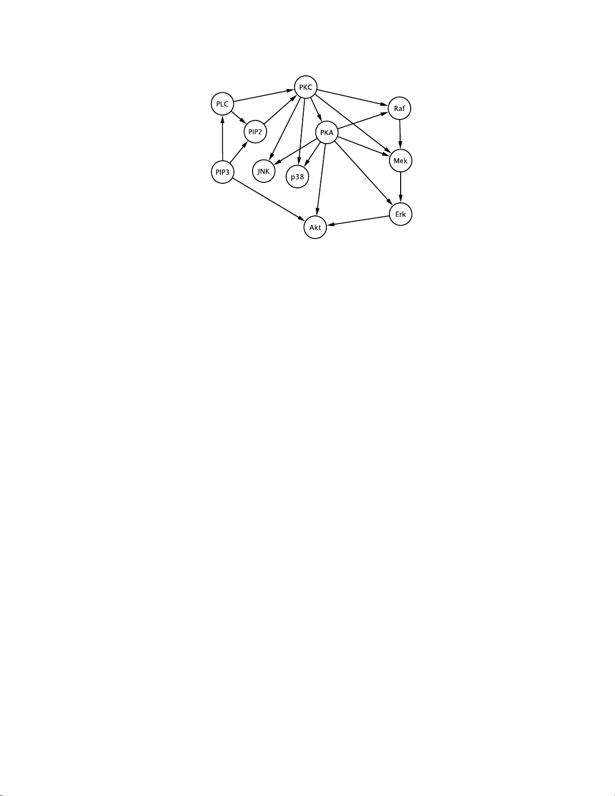
Multi-Domain Sampling Wit h Applications to Structur al Inference of Ba y esi an Net w orks ∗ Qing Zhou † Abstract When a posterio r distribution has m ultiple mo de s , unconditional exp ectations, such as the posterio r mean, ma y not oﬀer inf ormative summ aries of the distribution. Mo- tiv ated by this problem, we prop ose to decomp ose the sample s pace of a mult imo dal distribution into domains of attra ction of lo cal mo des. Domain-based representations are deﬁned to summarize the probabilit y masses of and c o nditional exp e c tations on domains of a ttraction, which are mu ch more informative than the mean and other unconditional expecta tio ns. A computational method, the m ulti-do main sampler, is de- veloped to construct domain- ba sed repres ent ations for an ar bitrary m ultimoda l distri- bution. The m ulti-domain sampler is applied to structural lea rning of pr otein-signa ling net works from high-thr oughput sing le-cell data, where a signaling netw ork is mo deled as a causal Bay es ian netw ork. Not only do es our metho d provide a detailed la ndscap e of the p os terior distribution but also improves the accurac y and the predictive p ow er of estimated net works. Key words: Domain-based representation; Multimo dal distributio n; Mo nt e Carlo ; Net w ork structure; Protein-signaling ne tw ork; W ang-Landa u alg orithm. 1 In tro duction In Ba yesia n inference the information on an unkn o wn parameter θ giv en an obser ved dataset y obs is con tained in the p osterior distribution p ( θ | y obs ). When a p osterior distribu tion ∗ T o appear in Journal of the Americ an St atistic al Asso ciation . † Qing Zhou is Assistan t Professor, D epartment of Statistics, Universit y of Calif ornia, Los Angeles, CA 90095 (Email: zhou@stat.ucla.edu). This wo rk was supp orted in part b y NSF grant DMS-0805491 and NS F CAREER Award DMS-1055286. T he author thanks the editor, the associate editor, and the tw o referees for helpful comments and sugge stions which signiﬁcantly improv ed the manuscript. 1 do es not b elong to a we ll-c haracterized family of distrib utions, Mark ov chain Monte C arlo (MCMC) is a standard computational approac h to Ba y esian inference via sampling fr om the p osterior distribution. T ypical examples of MCMC includ e th e Metrop olis-Ha stings (MH) algorithm (Metropolis et al. 1953 , Hastings 1970) and the Gibbs sampler (Geman and Geman 1984, Gelfand and Smith 1990, T anner and W ong 1987). Thorough reviews of recen t dev elopmen ts on Mon te Carlo m etho ds and th eir applications in Bay esian compu ta- tion can b e found in Chen et al. (2001 ) and Liu (2008). The p osterior mean E ( θ | y obs ) and other exp ectations are usually ap p ro ximated from a Mon te Carlo sample to su mmarize the p osterior distrib u tion. How ev er, th ese un conditional exp ectations may not oﬀer go o d summaries of the information for Ba yesian in ference when a p osterior distrib ution has mul- tiple lo cal mo des. O n e can easily construct a multimodal p osterior d istribution of w hic h the mean is lo cated in a lo w-densit y region and th us using it as an estimator for θ lac ks a con ven tional in terpretation. T o extract more information conta ined in a m ultimo dal p oste- rior distribution, it is desired to iden tify all ma jor mo des and calculate v arious statistics in appropriate neighborh o o ds of these mo d es. T o ac h iev e these tasks, w e pr op ose to p artition the sample space of θ in to a collection of domains suc h that the p osterior distribution restricted to eac h domain is unimo d al. The most parsimonious partition that minimizes the num b er of domains is to us e th e domains of attractio n (to b e deﬁned rigorously later) of the lo cal mo des. T ak e the trimo dal distribution p ( θ ) in Figure 1 as an illustration. The space is partitioned into three d omains, denoted b y Θ 1 , Θ 2 and Θ 3 : Each domain con tains exactly one lo cal m o de; if we mo v e any θ ∈ Θ k ( k = 1 , 2 , 3) along the tra jectory that alwa ys follo w s the gradient direction of p ( θ ), it will ev entually reac h the mo d e in the d omain Θ k . W e may then calculate v arious conditional exp ectations on th ese domains, E [ h ( θ ) | θ ∈ Θ k ] ( k = 1 , 2 , 3), for diﬀeren t functions h . T ogether with the probabilit y masses of the domains, P ( θ ∈ Θ k ), they pro vide more informativ e summaries of th e distribu tion p ( θ ) than unconditional exp ectations. Suc h a summary is called a d omain-based representati on (DR) for p ( θ ). Although desired, constru ction of DRs for an arbitrary d istribution is very challe nging in pr actice. Suﬃcient Mont e Carlo samples fr om domains of all lo cal mo des are necessary for estimating DRs, but eﬃcien t sampling from a m u ltimo dal distribution h as alw a ys b een a 2 −1 −1 −1 −5 −5 −5 −10 −20 −20 −20 −30 −30 −30 −40 −40 −40 −6 −4 −2 0 2 4 6 −6 −4 −2 0 2 4 6 A B C Figure 1: Contour plot of a t wo-dimensional d ensit y with three mo des lab eled A, B and C. The n um b ers rep ort log d ensities of con tours and the dash ed cu rv es mark the b ou n daries b et w een domains of attractio n. hard pr oblem. In this article, w e develo p a computational m etho d th at is able to construct domain-based representati ons for an arbitrary multimodal d istribution. W e p artition the sample space into domains of attraction an d u tilize an iterativ e weigh ting scheme aiming at sampling from eac h d omain with an equal frequ en cy . Th e w eigh ting sc heme was p rop osed b y W ang and Land au (2001), an d furth er dev elop ed and generalized by Liang (2005), Liang et al. (2007) and A tc had´ e and Liu (2010) among others. Ho w ever, a d irect application of these existing metho ds cannot provide accurate estimation of DRs, d ue to at least t wo reasons. First, sample s pace partition used in these m etho ds is usually predetermined according to a set of selected density lev els. But partitioning the space into domains of attractio n, as employ ed in our metho d, cannot b e completed b eforehand b ecause it is a non trivial j ob to detect all lo cal mo des and their domains in real applications. Second, the ab o ve metho ds mostly r ely on simple lo cal mov es and lac k a coherent global mov e to jump b et ween diﬀerent local mo des. T o obtain accurate estimation of DRs, we prop ose a dyn amic sc heme to partition the sample sp ace int o d omains of attraction and devise a global mo ve th at utilizes estimated DRs along sampling iterations to enable fast transitions b et w een m ultiple domains. Since the main feature of our metho d is to sample fr om m ultiple domains and construct DRs, we call it th e m ulti-domain (MD) sampler. The MD sampler can b e applied to a wide range of Ba y esian inference problems and 3 it is particularly p ow erful in tac kling problems with complicated p osterior distribu tions. Although there are many such applications in diﬀerent ﬁ elds, this article mainly concerns structural learning of causal Ba yesia n netw orks f rom exp erimental data. Learning net w ork structure via Mon te Carlo samp lin g is v ery challe nging as the multimodality of the p osterior distribution is extremely sev ere (F r iedman and Koller 2003 , E llis and W ong 2008 , L iang and Zhang 2009). In this p roblem, a domain of attractio n is deﬁn ed by a set of netw ork stru c- tures, eac h repr esen ted by a dir ected acyclic grap h (D AG) . In a sense, the goal of the MD sampler is to construct a detailed land scap e of th e p osterior distribution, whic h can p ro vide new insight s into the structural learnin g problem. Application of our metho d to a scien tiﬁ c problem is illustrated by a study on constru cting protein-signaling net w orks from s ingle-cell exp erimenta l data. A living cell is highly resp onsiv e to its en vironmen t d ue to th e exis- tence of widespread and d iv erse signal transdu ction path w a ys. These path w a ys constitute a complex signaling net w ork as cross-talks usually exist b etw een them. K no wledge of the structure of this n et work is critical to the understand ing of v arious cellular b ehavio rs and h uman diseases. Recen t adv ances in b iotec hnology allo w the b iologist to measure the states of a collect ion of molecules on a cell-b y-cell basis. Su c h large-scale data conta in ric h infor- mation for statistical inference of signaling net w orks, bu t p o w erful computational metho ds are needed giv en the complexit y in the lik elihoo d fu nction and th e p osterior d istribution. With the MD s amp ler, n ot only can w e bu ild a s ignaling netw ork from th e p osterior mean graph, but also we ma y disco v er new path w a y conn ections rev ealed by diﬀerent domains of the p osterior distribu tion, which are not accessible by other approac h es. The remaining p art of this article is organized as follo ws . Section 2 deﬁn es the domain of attraction and domain-based representa tion. In Section 3 w e d ev elop the MD samp ler and its estimation of DRs, with con v ergence and ergo dicit y of th e sampler established in App en d ix. The metho d is tested in Section 4 on an example in Euclidean space and implemen ted in Section 5 for Ba yesian inference of net w ork structure with a sim ulation study . Section 6 is the main application to the construction of signaling n et works in h uman T cells. Th e article concludes with a discussion on related and f u ture works. 4 2 Domain-based represen tation Let p ( x ), x ∈ X ⊆ R m , b e the den sit y of the target distribution. S upp ose that p ( x ) is diﬀeren tiable and denote by ∇ p ( x ) the gradien t of p at x . Deﬁne a diﬀerential equation d x ( t ) dt = ∇ p ( x ( t )) (1) and wr ite a solution path of this equation as x ( t ) , t ∈ [0 , ∞ ), where x (0) is a chosen initial p oint. Under some mild regularit y conditions, x ( ∞ ) con ve rges to a lo cal mo de of p ( x ), which is th e basic intuition b ehind the gradient descent algorithm to maximize p ( x ). Denote b y { ν 1 , . . . , ν K } all the lo cal mo d es, includin g the global mo de, of p ( x ). F or x ∈ X , let x (0) = x and d eﬁne the domain partition index by I ( x ) =      k , if x ( ∞ ) = ν k , f or k = 1 , . . . , K 0 , otherwise. (2) It maps x to the index of the lo cal mo de to whic h the solution path starting at x con v erges. Deﬁnition 1. Th e d omain of attraction of ν k is D k = { x ∈ X : I ( x ) = k } for k = 1 , . . . , K . F or simplicit y w e may call D k an attractio n domain or a d omain of p . If the stationary p oints of p ( x ) ha v e zero probability mass, then { D k : k = 1 , . . . , K } form a partition of th e sample space X except for a s et of zero p robabilit y mass. This is the d efault setting for this article. Let h ( x ) b e a p -in tegrable fu nction of x . W rite the probabilit y mass of D k and the conditional exp ectation of h ( X ) giv en X ∈ D k as λ k = P ( X ∈ D k ) = Z D k p ( x ) d x , (3) µ h,k = E [ h ( X ) | X ∈ D k ] = 1 λ k Z D k h ( x ) p ( x ) d x , (4) resp ectiv ely , for k = 1 , . . . , K . Deﬁnition 2. Th e domain-based represent ation of h w ith resp ect to the distribution p is a 2 × K array , D R p ( h ) = { ( µ h,k , λ k ) : k = 1 , . . . , K } . 5 The DR is equiv alent to the probabilit y mass function of E [ h ( X ) | I ( X )] that assigns probabilit y λ k to µ h,k for k = 1 , . . . , K . It p ro vides the exp ectation E [ h ( X )] = P k λ k µ h,k and the d ecomp osed con tributions from the attractio n domains of p ( x ). S uc h a represen- tation give s an informative lo w-dimensional summary of a multimodal distribution. F or a complex distribution with man y lo cal mo des, how ev er, we cannot aﬀord to estimate ( µ h,k , λ k ) f or ev ery domain when K is to o large and are less in terested in domains of negli- gible probabilit y masses ( λ k v ery clo se to ze ro). Du e to these reasons we deﬁne d omain-based represent ations with resp ect to a set of lo cal mo des { ν k : k = 1 , . . . , M } . Ind ex all the lo cal mo des as ν 1 , . . . , ν M , . . . , ν K ( M ≤ K ). Deﬁne th e d omain p artition ind ex with resp ect to { ν k } M k =1 b y I M ( x ) = I ( x ) if 1 ≤ I ( x ) ≤ M and I M ( x ) = 0 otherwise. Th en the sample space X can b e partitioned into D k = { x ∈ X : I M ( x ) = k } for k = 0 , . . . , M , where D k is the domain of ν k ( k ≥ 1) and D 0 = X − S M k =1 D k . Th e DR of h with r esp ect to { ν k } M k =1 is d eﬁned by the array { ( µ h,k , λ k ) : k = 0 , . . . , M } , where λ 0 and µ h, 0 are deﬁ ned for D 0 similarly as in Equations (3) and (4), r esp ectiv ely . Note that one can still obtain E [ h ( X )] = P M k =0 λ k µ h,k after merging D M +1 , . . . , D K in to D 0 . There is a geometric in terpretation for the attraction d omains of a p osterior d istribu- tion. Supp ose that Y = ( Y 1 , . . . , Y n ) is a sample from an u nkno wn d istribution ψ ( y ). W e assume a parametric family f θ = f ( · | θ ), θ ∈ Θ , as the mo del for Y and pu t a prior π ( θ ) on the unkn o w n parameter θ . The p osterior distribu tion of θ is giv en by p ( θ | Y ) ∝ π ( θ ) n Y i =1 f ( Y i | θ ) ≈ e nE [log f ( Y 1 | θ )] when the sample size n is large, where E [log f ( Y 1 | θ )] = R log[ f ( y | θ )] ψ ( y ) d y . Denote the K ullbac k-Leibler (KL) div ergence b et ween ψ and f θ b y d K L ( ψ k f θ ) = Z log  ψ ( y ) f ( y | θ )  ψ ( y ) d y . Then, p ( θ | Y ) ∝ exp[ − nd K L ( ψ k f θ )] when n is large. In the sp ace of densit y fun ctions, w e can regard d K L ( ψ k f θ ) as the “distance” to the p oin t ψ f rom a p oint in the manifold M = { f θ : θ ∈ Θ } . Note th at ψ is not n ecessarily in M if our mo del assumption on Y is 6 incorrect. Then p ( θ | Y ) m a y b e interpreted as a Boltzmann distribu tion on the manifold M und er a p oten tial ﬁeld nd K L ( ψ k f θ ). This p oten tial push es every f θ , indexed b y θ , to wards ψ , and the collection of θ wh ic h will b e drive n to an id en tical stationary p oint in M forms an attraction d omain of p ( θ | Y ). 3 The m ulti-domain sampler T o dev elop an algorithm that is able to construct domain-based represent ations with resp ect to the target distribu tion p , it is necessary to ident ify the attraction domain of an y x ∈ X . When p ( x ) is d iﬀeren tiable, this can b e ac h iev ed b y application of the gradient descent (GD) algorithm that ﬁ nds lo cal mo d es of p ( x ), or log p ( x ) for computational conv enience. Generalizati on to the space of net w ork stru ctures will b e discussed later. A n aiv e tw o-step approac h to the construction of DRs is quite ob vious. W e ma y ﬁrst apply a Mont e Carlo algorithm to simulate a sample { X t } n t =1 from p ( x ) or f rom a diﬀuse v ersion of p ( x ), e.g., [ p ( x )] 1 /τ for τ > 1 as used in parallel temp ering (Gey er 1991). Th en , for every t we determine I ( X t ) b y a GD searc h initiated at X t to ﬁ nd to w hic h domain it b elongs. This approac h partitions the sample into attraction domains so th at w e can estimate the pr obabilit y masses and conditional exp ectati ons for all identiﬁed domains. Although s im p le to imp lemen t, this t wo-step app roac h has a few d ra wbac ks in terms of eﬃciency . Without a careful and s p eciﬁc d esign the Mon te Carlo algorithm, ev en targeting at a diﬀuse v ersion of p ( x ), ma y n ot generate enough samples from all m a jor domains or ma y completely m iss some mo des. As a result, estimation on some attraction domains m ay b e inaccurate or u na v ailable. In add ition, this approac h d o es n ot utilize the inform ation on the target distribution pr o vid ed by the constru cted DRs. T o ov ercome these dra wbac k s , w e d ev elop the MD samp ler that ma y ac hiev e sim u ltaneously an eﬃcient sim ulation from a m ultimo d al distrib ution an d an accurate construction of domain-based repr esen tatio ns, with comparable computational complexit y as the naiv e t w o-step app roac h . 7 3.1 The main algorit hm W e wish to s amp le su ﬃcien tly f rom the ma jorit y of attrac tion domains. Ho wev er, the densit y at the b oundary b et ween t wo neigh b oring domains is often exp onen tially lo w (e.g., Figure 1), which mak es it diﬃ cu lt for an MH algorithm or a Gibbs sampler to jump across m ultiple domains. Thus, we need to allo w the s ampler to generate enough s amples from suc h lo w-d ensit y regions that connect diﬀerent d omains. These considerations motiv ate the follo wing double-partitioning d esign in the MD sampler. Supp ose that w e are giv en a set of lo cal mo d es of p ( x ), { ν 1 , . . . , ν M } , whic h ma y include the global mo de. Given ∞ = H 0 > H 1 > . . . > H L = −∞ , deﬁn e the d en sit y partition index J ( x ) = j if log p ( x ) ∈ [ H j , H j − 1 ) for j = 1 , . . . , L . W e partition the space X into ( M + 1) × L subr egions, D k j = { x ∈ X : I M ( x ) = k , J ( x ) = j } , k = 0 , . . . , M , j = 1 , . . . , L , (5) where I M ( x ) is the domain partition ind ex with resp ect to { ν k } M k =1 . Then, the attractio n domain of the lo cal mo d e ν k is D k = S j D k j (1 ≤ k ≤ M ). Note that some D k j ma y b e empt y; if log p ( ν k ) < H i then all D k j for j ≤ i are empty . In w hat follo ws, we only consid er nonempt y sub regions. F o r a given matrix W = ( w k j ) ( M +1) × L , deﬁn e a w orking densit y p ( x ; W ) ∝ M X k =0 L X j =1 p ( x ) 1 ( x ∈ D k j ) exp( w k j ) , (6) where 1 ( · ) is an indicator function. Let W ∗ = ( w ∗ k j ) such that exp( w ∗ k j ) = R D kj p ( x ) d x . Then, the probabilit y m asses of D k j are id en tical un der p ( x ; W ∗ ). Sampling from p ( x ; W ∗ ) has t wo immediate implicatio ns. First, the sample sizes on the attrac tion d omains, { D k } M k =1 , will b e comparable, and thus, d omain-based rep resen tations can b e constructed with a high accuracy . Note that commonly used MCMC s tr ategies for multimod al distrib u tions, such as temp ering, cannot generate samples of comparable sizes from diﬀeren t d omains. Second, the samp ler will stay in lo w-densit y regions (e.g., D k L ) for a sub stan tial fraction of time, whic h mak es it p ractically p ossible to ju mp b etw een d omains. C on v ersely , d omain-based represent ations ma y b e utilized to design eﬃcient lo cal and global mo ves for samplin g f r om 8 p ( x ; W ∗ ). W e m a y construct online estimate of the co v ariance matrix on the d omain of a lo cal mo de, which can b e us ed for tu ning the step s ize of a lo cal mo ve in this d omain. F or a m ultimo dal distrib u tion, tu ning step size f or eac h domain is m ore useful than tunin g the ov erall step size (Harrio et al. 2001) . On ce w e h a ve identiﬁed suﬃcien t local mo des and estimated co v ariances of their resp ectiv e d omains, we can us e them to d esign global mo ves th at ma y jump from one domain to another. As one can see, these p rop osals can b e implemen ted only if w e hav e partitioned samples into attraction domains. F or x , y ∈ X , let q ( x , y ) b e a prop osal fr om x to y and r ( x ; θ , V ) a distribu tion with p arameters θ and V ∈ V . W e ﬁ rst dev elop the main algorithm of the MD sampler, assuming that the d ensit y ladder { H j } is ﬁxed and M lo cal mo des { ν k } M k =1 ha v e b een iden tiﬁed. Dynamic up date of th ese p arameters will b e discuss ed in Section 3.2 as the burn -in algorithm. Let g k ( x ) b e a map from X to V for k = 1 , . . . , M . Algorithm 1 (The main algorithm) . Initialize W 1 = ( w 1 k j ), parameters V 1 k ∈ V ( k = 1 , . . . , M ), p mx ∈ [0 , 1), and X 1 ∈ X . Set γ 1 ≤ 1. F or t = 1 , . . . , n : 1. Dra w Y from q ( X t , y ) with probabilit y (1 − p mx ) or from th e mixtur e distrib ution 1 M P M k =1 r ( y ; ν k , V t k ) w ith probab ility p mx . 2. Determine the dens ity p artition ind ex J ( Y ) and p erform a GD searc h initiated at Y to determine the domain partition in dex I M ( Y ). 3. Accept or r eject Y according to the MH ratio targeting at p ( x ; W t ) to obtain X t +1 . 4. F or k = 0 , . . . , M and j = 1 , . . . , L up d ate w t +1 k j = w t k j + γ t 1 ( I M ( X t +1 ) = k , J ( X t +1 ) = j ) , (7) for k = 1 , . . . , M up date V t +1 k = V t k + γ t 2  g k ( X t +1 ) − V t k  1 ( I M ( X t +1 ) = k ) , (8) and d etermine γ t +1 . 9 W e ma y regard w t k j as a weigh t for the subregion D k j . After eac h visit to D k j , the w eigh t w t +1 k j increases by γ t unit (7 ), which decreases the p r obabilit y m ass of D k j under the w orking densit y p ( x ; W t +1 ) (6 ). Such a wei gh tin g sc heme aims to visit ev ery D k j uniformly . There are t w o t ypical choice s of { γ t } . The ﬁr st c hoice follo ws the standard design in sto c h astic appr o ximation whic h emplo y s a predetermined sequence s uc h th at P ∞ t =1 γ t = ∞ and P ∞ t =1 γ ζ t < ∞ f or ζ ∈ (1 , 2) (And rieu et al. 2005, Andrieu and Moulines 2006, Liang et al. 2007). The second d esign, originally pr op osed by W ang and Landau (2001), adjusts γ t in an adaptiv e wa y . How ev er, there is diﬃcult y in establishing its conv ergence (A tchad ´ e and Liu 2010), an d th us we adopt a mo diﬁed W ang-Landau (MWL) d esign to up date { γ t } in the MD sampler. Initialize c 1 k j = 0 for all k and j in Algorithm 1 . The MWL up date at iteration t ( t = 1 , . . . , n ) is giv en b elo w. Routine 1 (MWL up date) . If γ t < ǫ γ , set γ t +1 = γ t ( γ t + 1) − 1 ; otherwise: • Set c t +1 k j = c t k j + 1 ( X t +1 ∈ D k j ) f or all k , j and calculate ∆ c t +1 max = max k ,j | c t +1 k j − ¯ c t +1 | , where ¯ c t +1 is th e a v erage of all c t +1 k j . • If ∆ c t +1 max ≥ η ¯ c t +1 , set γ t +1 = γ t ; otherwise, set γ t +1 = ργ t and c t +1 k j = 0 for all k , j . That is, if γ t ≥ ǫ γ w e decrease γ t ( ρ < 1) only when the samp ler has visited ev ery subregion D k j with a roughly equal frequency since our last mo diﬁ cation of γ t . Let t c = min { t : γ t < ǫ γ } . F or t > t c the up date b ecomes deterministic with γ t = 1 / ( t + ξ ), wh ere ξ = γ − 1 t c − t c . The default setting for all th e resu lts in th is article is giv en by ρ = 0 . 5, η = 0 . 25 and ǫ γ = 10 − 4 . Under s ome regularit y conditions and the MWL u p d ate of { γ t } , exp( w n k j ) a.s. − → Z D kj p ( x ) d x = exp( w ∗ k j ) , (9) after b eing normalized to su m up to one, V n k a.s. − → R D k g k ( x ) p ( x ; W ∗ ) d x R D k p ( x ; W ∗ ) d x ∆ = V ∗ k , (10) 1 n n X t =1 h ( X t ) a.s. − → Z X h ( x ) p ( x ; W ∗ ) d x , (11) 10 as n → ∞ . S ee Theorem 2 in App en d ix for m ore details. If X ⊆ R m , w e often c h o ose g k ( x ) = ( x − ν k )( x − ν k ) T so that V ∗ k is close to the cov a riance matrix of the conditional distribution [ X | X ∈ D k ], where X ∼ p ( x ; W ∗ ). W e u se the m o de ν k instead of the mean b ecause the mo de can b e obtained accurately via a GD algorithm. The use of γ t / 2 ( < 1) in Equation (8) ensur es that V t +1 k is p ositiv e deﬁn ite if V t k is p ositiv e deﬁnite. There are t w o t yp es of pr op osals in step 1 of the algorithm, a lo cal prop osal q ( X t , y ) and a mixture distrib ution p r op osal. One adv antag e of p artitioning samples int o attraction domains is em b o died in the mixtur e distr ibution prop osal, in w h ic h we ran d omly d ra w a domain partition index k ∈ { 1 , . . . , M } and then p rop ose a samp le Y from r ( y ; ν k , V t k ). Equal mixture prop ortions (1 / M ) are used b ecause a u niform s amp ling across domains is preferred. The default c hoice of the distribu tion r ( y ; ν k , V t k ) in R m is N ( ν k , V t k ) for k = 1 , . . . , M , wh ic h giv es a mixture normal pr op osal that matc h es the mo de and the co v ariance on eac h domain of th e working target p ( x ; W t ). Th is pr op osal uses a mixture distr ib ution to appr o ximate the multi mo dal target . It can generate eﬃcien t global jum ps from one domain to another if p ( x ; W t ) on the domain D k can b e w ell appr oximate d by r ( x ; ν k , V t k ) with the identiﬁed mo de ν k and the estimated V t k . F or simp licit y we call th is prop osal the mixe d jump . The t yp ical design for q ( X t , y ) in R m is to p rop osal Y ∼ N ( X t , σ 2 I ), where σ 2 is a scalar and I is the identi t y matrix. Ho wev er, wh en the co v ariances are ve ry diﬀerent b et w een d omains, usin g a single lo cal prop osal ma y cause h igh auto correlation, since the step size migh t b e either to o big for domains with small co v ariances or to o small for those with large co v ariances, or b oth. In this case, w e m ay incorp orate an adaptiv e lo cal pr op osal, Y ∼ N ( X t , σ 2 V t I M ( X t ) ), in addition to q ( X t , y ), suc h that th e learned co v ariance structure of a domain is u tilized to guide the lo cal prop osal. Th is s h o w s another adv antag e of the domain-partitioning d esign. Remark 1. W e summarize the un ique features of the main algorithm. First, d omain parti- tioning is incorp orated in the framewo rk of the W ang-Landau (WL) algorithm. T his allo ws a more uniform sampling from diﬀeren t domains, which facilitate s constr u ction of DRs. A t eac h iteration, a GD searc h is employ ed to determine I M ( Y ) and thus the computational complexit y of this algorithm is comparable to the naiv e t wo- step appr oac h. Second, an 11 adaptiv e global mov e, the m ixed j ump, is p r op osed given DRs constr u cted along the iter- ation, wh ic h utilizes identi ﬁed mo d es and learned co v ariances to ac hieve b etw een-domain mo ves. Remark 2. V eriﬁcation of the regularit y conditions f or con v ergence of the algorithm (see App end ix) is recommended b efore application. F urthermore, we suggest a few conv ergence diagnostics that can b e con v en iently us ed in pr actice. First, γ n should b e small enough at the ﬁn al iteration and th e fr equ ency of visiting diﬀerent D k j should b e roughly ident ical. Second, W n and V n k should h a ve conv erged with an acceptable accuracy . Violatio ns of these tw o criteria indicate that more iterations ma y b e necessary . Thir d, the adaptiv e parameters used in the mixed ju mp ( V t k ) should alwa ys stay in a reasonable range. F or example, if V t k is a co v ariance matrix, one ma y c h ec k whether its eigen v alues are close to zero or unreasonably large, whic h ma y indicate d iv ergence of the cur ren t ru n. If the last criterion is not satisﬁed, it is suggested to reinitialize the MD sampler with a smaller γ 1 . 3.2 The burn-in algorithm In practical applications of the MD sampler, the density ladd er { H j } and th e lo cal mo des { ν k } are up d ated dynamically in a burn -in p erio d b efore the main algorithm (Algorithm 1). The d ynamic up dating sc hemes are crucial steps for constru cting d omain-based representa - tions in r eal applica tions, as one cannot partition th e sample sp ace in to domains of attraction b eforehand . W e set H 1 , . . . , H L − 1 as an ev enly spaced sequence so that ∆ H = H j − H j +1 is a constan t for j = 1 , . . . , L − 2. Let { H t j } b e the densit y ladder and Λ t = { ν t k : k = 1 , . . . , M t } b e the set of M t iden tiﬁed mo d es at iteration t . Let K ∗ b e the maxim um n um b er of mo d es to b e recorded and d en ote b y ν ( x ) the m o de of the d omain th at x b elongs to. Let 0 b e the zero matrix with dimen sion determined by the con text. The follo wing routine is used to up d ate Λ t when a new sample Y is prop osed. Routine 2. Let s t = argmin 1 ≤ k ≤ M t p ( ν t k ). • If ν ( Y ) 6∈ Λ t and M t < K ∗ , set Λ t +1 = Λ t ∪ { ν ( Y ) } , M t +1 = M t + 1, and initialize w t M t +1 j = 0 for all j ; 12 • if ν ( Y ) 6∈ Λ t , M t = K ∗ and p ( ν ( Y ) ) > p ( ν t s t ), set ν t +1 s t = ν ( Y ) , ν t +1 k = ν t k for k 6 = s t , M t +1 = M t , and assign w t 0 j ⇐ w t 0 j + w t s t j and w t s t j ⇐ 0 f or all j . • otherwise set Λ t +1 = Λ t and M t +1 = M t . According to this r outine, w e record at most the K ∗ highest mo des iden tiﬁed d uring the bu r n-in p erio d . If there are more than K ∗ mo des, Algorithm 1 will construct DRs with resp ect to the recorded mo des. The w eigh ts ( w t k j ) are up dated when a new mo de r ep laces an old one in Λ t , for whic h the assignment op erator ‘ ⇐ ’ is used to distinguish from equalit y . The density ladd er { H t j } is adju sted suc h that H t 1 , the lo wer b ound of the highest densit y partition in terv al, is close to log u ∗ , wh ere u ∗ is the densit y of the highest m o de iden tiﬁed so far. If log u ∗ > H t 1 + ∆ H we mov e u p w ards the density ladder b y ∆ H unit and up d ate the w eigh ts ( w t k j ) accordingly , with details pro vided in Routine 3. This strategy h elps the samp ler to explore the h igh-d ensit y p art, whic h is imp ortan t for statistical estimation and ﬁ nding the global mo de. Routine 3. Giv en Λ t +1 , ﬁ nd u t +1 = max { p ( ν t +1 k ) : k = 1 , . . . , M t +1 } . • If log u t +1 > H t 1 + ∆ H , set H t +1 j = H t j + ∆ H for j = 1 , . . . , L − 1; for k = 0 , . . . , M t +1 , assign w t k L ⇐ w t k ( L − 1) + w t k L , w t k j ⇐ w t k ( j − 1) for j = L − 1 , . . . , 2, and w t k 1 ⇐ 0; • otherwise set { H t +1 j } = { H t j } . Algorithm 2 (The bur n-in algorithm) . I n put L, ∆ H and K ∗ . Set γ 0 = 1. Initialize X 1 ∈ X , Λ 1 = { ν ( X 1 ) } , M 1 = 1, W 1 = ( w 1 k j ) 2 × L = 0 , and V 1 1 . S et H 1 1 = log p ( ν ( X 1 ) ) and H 1 j = H 1 j − 1 − ∆ H for j = 2 , . . . , L − 1. F or t = 1 , . . . , B : 1. Dra w Y ∼ q ( X t , y ) and ﬁnd ν ( Y ) b y a GD search. 2. Giv en ν ( Y ) , up date Λ t +1 and M t +1 b y Routine 2 ; if ν t +1 ℓ = ν ( Y ) is a new mo de in Λ t +1 , in itialize V t ℓ . Giv en Λ t +1 , u p d ate { H t +1 j } by Routine 3. 3. Giv en Λ t +1 and { H t +1 j } , accept or r eject Y with the MH ratio targeting at p ( x ; W t ) to obtain X t +1 . 4. Execute step 4 of Algorithm 1 with γ t = γ 0 . 13 Remark 3. Note that γ t = 1 for ev ery iteration in th e b urn-in algorithm. Th is pushes the sampler to explore diﬀeren t regions in the samp le space so that more lo cal m o des can b e iden tiﬁed. I n this case, the we igh t w t k j records the num b er of visits to D k j b efore the t th iteration, which is the reason for our up dating sc hemes on { w t k j } in Routine 2 when a mo d e is up dated in Λ t +1 and in Routine 3 wh en the d ensit y ladder c hanges. Remark 4. The bu rn-in algorithm can b e used as an optimization metho d that s earches for up to K ∗ lo cal mo des of the highest densities. As demonstr ated in the Ba y esian n et work applications, this algorithm is v ery p o werful in ﬁnding global mo des. The MD samp ler requires only a few input p arameters, L, ∆ H , p mx , and K ∗ . A practical rule is to c ho ose L and ∆ H such that the range of the densit y partition in terv als, L ∆ H in log scale, is wide enough to co ver imp ortan t regions. In this p ap er, w e set L ∆ H around 20 for the lo w-dimensional test example in Secti on 4 a nd around 20 0 for le arning Ba ye sian netw orks in Sections 5 and 6. By default the probabilit y of pr op osing a mixed jump p mx = 0 . 1. The eﬀect of k eeping only K ∗ mo des will b e studied later with the examples. 3.3 Statistical estimation The domain-based representat ion of h is constructed by estimating λ k (3) and µ h,k (4) f or k = 0 , . . . , M w ith p ost bur n-in samples, den oted by { X t +1 } n t =1 . Let k t = I M ( X t +1 ), j t = J ( X t +1 ), a t = P k ,j exp( w t k j ), and exp( ˜ w t k j ) = exp( w t k j ) /a t suc h that P k ,j exp( ˜ w t k j ) = 1. The key ident it y for our estimation is P ∞ t =1 h ( X t +1 ) exp( ˜ w t k t j t ) P ∞ t =1 exp( ˜ w t k t j t ) a.s. − → Z X h ( x ) p ( x ) d x , (12) whic h f ollo ws from (11) as exp( ˜ w t k t j t ) a.s. − → exp( w ∗ k t j t ) ∝ p ( X t +1 ) /p ( X t +1 ; W ∗ ) asymptoti- cally (9). S ee Liang (2009) and A tc had´ e and Liu (2010 ) for similar results. How ev er, ˜ W t = ( ˜ w t k j ) ma y b e far from W ∗ ev en for p ost bur n-in iterations. Thus, it is desired to use a weigh ted v ersion of (12) s o that X t +1 will carry a higher w eigh t if ˜ W t is closer to W ∗ . S ince decrease in γ t indicates con v ergence of the MD samp ler and a t +1 /a t a.s. − → e cγ t for c ∈ (0 , 1) (supp lemen tary do cument), a reasonable c h oice is to weigh t X t +1 b y a t so that 14 unnormalized ( w t k j ) w ill b e u s ed in (12). Consequent ly , D R p ( h ) is constructed with ˆ λ k = P n t =1 1 ( X t +1 ∈ D k ) exp( w t k t j t ) P n t =1 exp( w t k t j t ) , ˆ µ h,k = P n t =1 h ( X t +1 ) 1 ( X t +1 ∈ D k ) exp( w t k t j t ) P n t =1 1 ( X t +1 ∈ D k ) exp( w t k t j t ) , for k = 0 , . . . , M . Then, µ h = E [ h ( X )] is estimated b y ˆ µ h = P k ˆ λ k ˆ µ h,k . Please see supplementary d o cument for more d iscussion on this w eigh ted estimation. In the next three sections we demonstrate the eﬀectiv en ess of the MD sampler in sta- tistical estimation, esp ecial ly estimation of DRs, compared to the naive t wo-step approac h. F or all examples, w e employ the WL algorithm with the MWL up d ate (Routine 1) as th e Mon te C arlo metho d in the tw o-step appr oac h. T o minimize hidden artifacts in a compar- ison due to co din g d iﬀerences, we imp lemen t the WL algorithm with th e same bu rn-in and main algorithms of the MD sampler. In th e main algorithm (Algorithm 1) w e r eplace th e up d ating scheme in Equation (7 ) with w t +1 k j = w t k j + γ t 1 ( J ( X t +1 ) = j ) (13) for k = 0 , . . . , M and j = 1 , . . . , L and mo dify the b urn-in algorithm accordingly , so that w t 0 j = · · · = w t M j ∆ = w t j for eve ry iteration. Consequent ly , the w orking den sit y is eﬀectiv ely p ( x ; W t ) ∝ L X j =1 p ( x ) 1 ( J ( x ) = j ) exp( w t j ) (14) as used in the WL algo rithm, which is a diﬀuse version of p ( x ) such th at eac h density partition inte rv al will b e equally s amp led after con vergence. Note that the same GD searc h is applied at eac h iteration to p artition samples in to attrac tion d omains for estimating DRs. Our comparison aims to highligh t the eﬀect of d omain partitioning and the mixed ju mp in the MD sampler whic h are the key diﬀerences from the WL algorithm. 15 4 A test example W e test the MD sampler with an example in R m . F or this example, domain-based repre- sen tatio ns can b e obtained via one-dimensional n umerical int egration with a high accuracy , whic h pr ovides the basis to ev aluate our estimation. W e choose K ∗ = 100, whic h is greater than the total n um b er of lo cal mo des, to construct complete DRs. Let x = ( x 1 , . . . , x m ). Th e R astrigin fun ction (Gordon and Whitley 1993) is deﬁn ed as R ( x ) = m X i =1 x 2 i + A " m − m X i =1 cos( π x i ) # , (15) where A is a p ositiv e constan t. W e set A = 2 and m = 4 in (15) to obtain our target distribution p ( x ) ∝ exp[ − R ( x )], whic h has 3 4 = 81 lo cal mo des f ormed b y all the elemen ts of the pro du ct set {− 1 . 805 , 0 , 1 . 80 5 } 4 . These lo cal mo des ha v e ﬁ v e distinct log densit y v alues, 0, − 3 . 62, − 7 . 24, − 10 . 87, and − 14 . 49, dep enden t on the com binations of their co ordinates. They are group ed accordingly in to ﬁv e la yers s o that th e n um b er of zeros and the num b er of ± 1 . 805 in the coordin ates of a local mo de at the k th la y er are (5 − k ) and ( k − 1), resp ectiv ely , for k = 1 , . . . , 5. The attracti on domains of lo cal mo des at the same la y er ha v e id en tical probabilit y masses and ident ical conditional means up to a p erm utation and c h ange of signs of th e co ordinates. W e app lied the MD sampler 100 times in dep end en tly , eac h ru n with L = 10 densit y partition interv als, ∆ H = 2, B = 50K burn-in iterations and a total of 5 million (M) iterations (in clud ing the burn-in iterations). Th e lo cal prop osal w as simply N ( X t , I ). The a verag e acceptance rate w as 0.26 for the lo cal mo ve and wa s 0.56 for the mixed jump . Let X = ( X 1 , . . . , X 4 ) and S = P i X i . W e estimated E ( X ), E ( e 2 S ), E ( Q i X i ), E ( P i X 5 i ), and E ( P i X 6 i ), all via d omain-based rep r esen tatio ns. Since the target d ensit y of this example is a pro d uct of one-dimensional marginal d en sities, the ab o ve exp ectat ions can b e calculated accurately through one-dimensional n umerical in tegration. W e compared our estimates from MD sampling w ith the results from numerical in tegration by computing mean squ ared errors (MSE s). W e rep ort the av erage MSE of the estimated log probabilit y masses (log λ k ) and the a v erage MSE of the estimated conditional means ( µ X ,k ) o v er all the lo cal m o des 16 T able 1: MSE comparison on the Rastrigin fun ction MSE RMSE MSE RMSE MSE RMSE MD WL MD 0 MD WL MD 0 MD WL MD 0 log λ 1 1.1e-5 1.93 2.24 µ X , 1 2.3e-4 0.83 2. 87 X 1.7e-4 1.22 3. 19 log λ 2 3.6e-3 2.35 2.47 µ X , 2 2.5e-4 2.88 2. 96 e 2 S 0.59 3.25 3.09 log λ 3 3.5e-3 4.64 3.22 µ X , 3 2.8e-4 6.16 3. 34 Q i X i 1.6e-9 2.84 2. 70 log λ 4 3.3e-3 8.63 3.92 µ X , 4 2.9e-4 12.0 4. 09 P i X 5 i 6.1e-3 2.71 2. 06 log λ 5 3.2e-3 16.8 4.66 µ X , 5 3.3e-4 21.1 5. 06 P i X 6 i 0.11 1.95 2.26 at th e same la y er ( k = 1 , . . . , 5), and for other fun ctions we only rep ort the MSEs of the estimated exp ectations to sav e space (T able 1). As a comparison, w e also applied the WL algorithm (as in the naiv e t w o-step approac h) to this problem with the same parameter setting. The ratio (RMSE) of the MSE of th e WL algorithm o v er th at of the MD sampler for eac h estimate is give n in T able 1. The WL algorithm sh o wed larger MS E s than the MD sampler for almost all the estimates, esp ecially for those on d omains at la yers 3, 4 and 5. F or example, the MD sampler w as at least 16 times more eﬃcien t than the WL algorithm for estimating log λ 5 and µ X , 5 . The WL algorithm did n ot sim ulate suﬃcient samples fr om these d omains, although it visited uniformly diﬀerent d en sit y partition in terv als. On the con trary , the double-partitioning design facilitated the MD sampler to explore every domain in a un iform manner, wh ich led to a substant ial imp ro v ement in estimation for these la y er s . This sho ws the critical role of d omain partitioning in estimating DRs. T o s tudy the eﬀect of the mixed jump, we re-applied the MD sampler with p mx = 0, and calculated the ratio of the r esulting MSE (MD 0 in T able 1) o ver that of the MD sampler with p mx = 0 . 1, the default setting. One sees an increase of tw o f olds or more in MSEs without the mixed jump. The con vergence of the MD sampler without the mixed jump b ecame slo w er , reﬂected by a ﬁv e-fold increase in γ n after the same num b er of iterations, a ve raging o v er 100 in d ep end ent runs. These observ ations demonstrate that the mixed jump s erv ed as an eﬃcien t global mov e whic h accele rated conv ergence of the MD sampler and impro v ed estimation accuracy . 17 5 Learning Ba ye sian net wo rks A Ba y esian net work (BN) factorizes the join t distribution of m v ariables Z = { Z 1 , . . . , Z m } in to P ( Z ) = m Y i =1 P ( Z i | Π G i ) , (16) where Π G i ⊂ Z is the parent set of Z i . A graph G is constructed to co d e the stru ctur e of a BN by connecting eac h v ariable (no de) to its c h ild v ariables via directed edges. F or (16 ) to b e a well-deﬁned joint distribution, the graph G must b e a DA G. W e consider the use of Ba y esian net works in causal inf erence (Spirtes, Glymour and S cheines 1993, P earl 2000), whic h is tightl y connected to man y areas in statistics, suc h as str u ctural equations, p oten tial outcomes, and randomization (Holl and 1988, Neyman 1990 , Ru bin 19 78, Robins 1986) . Here w e follo w Pea rl’s form ulation of causal netw orks by mo deling exp erimen tal inte rv en tion. I f Z j is a paren t of Z i in a causal Ba y esian net wo rk, then exp erimental in terven tions that c h ange the v alue of Z j ma y aﬀect the distribu tion of Z i , b u t not con versely . Once all the parents of Z i are ﬁxed b y inte rv en tion, the d istribution of Z i will not b e aﬀected b y in terv entio ns on any v ariables in the set Z \ (Π G i ∪ { Z i } ). I n the example causal net w ork of Figure 2, if w e ﬁx Z 1 and Z 3 b y exp erimental interv ent ion, then th e distribu tion of Z 4 will not b e aﬀected by p ertu rbations on Z 2 , Z 5 , or Z 6 . Figure 2: An example Bay esian n et work of six v ariables. 5.1 P osterior distribution W e fo cus on the discrete case where eac h Z i tak es r i states ind exed by 1 , . . . , r i and the paren ts of Z i tak e q i = Q Z j ∈ Π G i r j join t states. Let θ ij k b e the causal probabilit y for Z i = j giv en the k th j oint state of its parent s et. A causal BN with a giv en stru cture G is 18 parameterized by Θ = { θ ij k : P j θ ij k = 1 , θ ij k ≥ 0 } . W e in fer netw ork structure from t wo t yp es of data joint ly , exp erimental data and observ ational d ata. F o r exp erimen tal data, a subset of v ariables are known to b e ﬁxed by in terv entio n. Inferrin g causalit y with inte rv en tion h as b een extensively studied in v arious con texts (e.g., Robins 1986, 1987, P earl 1993). W e adopt C o op er and Y oo (1999) for calculating th e p osterior pr obabilit y of a net w ork stru cture given a mix of exp erimenta l and observ ational data. Su p p ose that N ij k is the n um b er of data p oin ts for whic h Z i is not ﬁ xed by interv en tion and is foun d in state j w ith its p aren t set in joint state k . Then, the collection of coun ts N = { N ij k } is the suﬃcien t statistic for Θ (Ellis and W ong 2008). Let | Π G i | b e the size of the parent set of Z i . Th e prior distribu tion o ver net w ork stru ctures is sp eciﬁed as π ( G ) ∝ β P i | Π G i | , β ∈ (0 , 1), which p enalizes graph s w ith a large num b er of edges. With a p ro du ct-Diric hlet prior for Θ , the p osterior distribu tion [ G | N ] (Co op er and Hersk o vits 1992) is P ( G | N ) ∝ m Y i =1    β | Π G i | q i Y k =1   Γ( α i · k ) Γ( α i · k + N i · k ) r i Y j =1 Γ( α ij k + N ij k ) Γ( α ij k )      , (17) where α ij k = α/ ( r i q i ) is the ps eu do count for the causal pr obabilit y θ ij k in th e pro d uct- Diric hlet p rior and N i · k = P j N ij k (similarly for α i · k ). Th e hyperp arameters in the prior distributions are c hosen as β = 0 . 1 and α = 1. 5.2 MD sampling ov er D AGs The space of DA Gs is discr ete in n ature. W e deﬁn e domains of attraction for P ( G | N ) (17) with a mov e set comp osed of addition, d eletion and reversal of an edge. Give n a D A G G a , w e say that another DA G G b is a neighb or of G a if G b can b e obtained via a single mo ve starting from G a , i.e., by add ing, deleting or rev ersing an edge of G a . Denote by ng b ( G a ) all the neighb ors of G a and let ng b ( G a ) = ng b ( G a ) ∪ { G a } . A D A G G ∗ is d eﬁned as a lo cal mo de of a probabilit y dens it y (mass) fu nction p ( G ) if p ( G ∗ ) > p ( G ′ ) for every 19 G ′ ∈ ng b ( G ∗ ). Let G 0 b e a DA G and deﬁne r ecursiv ely G t +1 = argmax G ∈ ng b ( G t ) p ( G ) , for t = 0 , 1 , . . . . (18) That is, we r ecur siv ely ﬁ nd the single mov e that leads to the greatest increase in p until a lo cal mo de is r eac hed, w h ic h can b e v iewed as a discrete coun terpart of the gradient descen t algorithm. If there are more than one maxim um in (18) with an identic al fu nction v alue, we tak e the ﬁrst maxim um according to a ﬁxed orderin g of the neigh b ors. W e call this r ecursion the steep est neigh b or ascen t (S NA). Based on SNA, we d eﬁne the domain p artition ind ex I ( G ) and the attraction domains of p in th e same manner as for a diﬀeren tiable d ensit y (Equation 2 and Deﬁnition 1). The target distribution in this application is the p osterior d istribution P ( G | N ) and w e deﬁne w orking densit y P ( G | N ; W ) similarly as in (6). T o implemen t the MD sampler for D AGs, we employ the m ov e s et as the lo cal p rop osal and develo p the follo wing mixed jump. F or a D AG G , we deﬁne an edge v ariable E G ij for ev ery p air of n o des Z i and Z j ( i < j ) such that E G ij = 1 if Z i is a parent of Z j , E G ij = − 1 if Z j is a parent of Z i , and E G ij = 0 otherwise. Giv en a D AG ν , let C ( G ; ν ) = ( C a ( G ; ν ) , C d ( G ; ν ) , C r ( G ; ν )) b e a map of G , where C a ( G ; ν ) = P i 0 is a small pr ior count added to eac h category . Analogously , if E ν k ij = 0 we prop ose E Y ij = 0 , 1 , or − 1 with probabilities prop ortional to ( T − | E k | − v t k ,a , v t k ,a / 2 , v t k ,a / 2) + b . Lastly , to ensur e a prop osed graph is acyclic, a c hec k for cycles is p erformed wh en w e pr op ose to add or rev erse an edge in either the lo cal prop osal or th e mixed j u mp. If the r esu lting graph is cyclic, w e supp r ess th e probability for the corresp ondin g m ov e. F ollo win g the common pr actice in str uctural learning of discrete BNs, w e set an up p er b ound for th e n um b er of paren ts (indegree) of a no d e. In all the follo wing examples and applications, this u pp er b oun d is chosen to b e four . W e are intereste d in the p osterior exp ected adjacency m atrix A = ( a ij ) m × m and its domain-based representat ion, where a ij (1 ≤ i, j ≤ m ) is the p osterior probabilit y for a directed ed ge from Z i to Z j . F or eac h iden tiﬁed lo cal mo de ν k , w e estimate the pr ob ab ility mass λ k of its attraction domain D k and the conditional exp ected adjacency matrix A k on the domain. Then, A is estimated b y ˆ A = P k ˆ λ k ˆ A k . 5.3 Sim ulation W e simulat ed data f r om t w o BNs, eac h of six binary v ariables ( m = 6 , r i = 2 , ∀ i ). This is the maximum num b er of no des for whic h w e can en u merate all D AGs, num b ering ab out four million, to obtain true p osterior distribu tions and domain-based repr esen tatio ns as the ground truth for testing a computational metho d. The ﬁrst net w ork h as a c hain structur e in which Z i is the only parent of Z i +1 for i = 1 , . . . , 5 and Z 1 has no p arent. T he second net work has a more complex structure sho wn in Figure 2. W e simulat ed 50 d atasets inde- p end ently from eac h netw ork. In eac h d ataset, 20% of the d ata p oin ts were generated with in terv entio ns. Please see su pplementa ry do cumen t for d ata simulati on details. The MD sampler w as app lied to the 100 datasets with L = 15, ∆ H = 10, p mx = 0 . 1, K ∗ = 100 and a total of 5M iterations with the ﬁrst 50K as bu r n-in iterations. T o v erify its 21 T able 2: Comparison on simulat ed data from tw o BNs MD MD 0 WL K ∗ = 10 MSE RMSE # of missed mo des 0 0 0 0.51 log ˆ λ k 0.028 1.48 5.06 0.48 ˆ A k 1.3e-4 1.6 5 11.0 0.99 ˆ A 1.3e-4 1.7 6 1.67 1.03 # of missed mo des 0 0 0.12 2.06 log ˆ λ k 0.029 401 136 8 0.84 ˆ A k 1.7e-4 2.9 6 13.6 1.01 ˆ A 1.5e-4 7.1 7 5.09 0.98 The top and b ottom p anels rep ort the results for th e c hain and th e graph n et works, r e- sp ectiv ely . F or eac h estimate, rep orted are the MSE of the MD s amp ler and th e RMSEs (ratios) of the other metho ds relativ e to the MD sampler. p erforman ce, we compared iden tiﬁ ed lo cal mo des, estimated pr obabilit y masses { log ˆ λ k } , conditional exp ected adjacency matrices { ˆ A k } , and exp ected adjacency matrix ˆ A to th eir resp ectiv e true v alues obtained via enumerating all D AGs. Our enumeratio n conﬁrm s that the p osterior d istr ibutions indeed h a ve m ultiple lo cal m o des. Th e c h ain and the graph (Figure 2) netw orks hav e on a ve rage 3.57 and 7.06 mo des o v er the s imulated datasets, resp ectiv ely , and the maximum num b er of mo des is 29 for the c h ain and 34 for the graph. As rep orted in T able 2, th e MD samp ler did n ot miss a sin gle lo cal mo de for an y dataset, whic h demonstrates its global searc h abilit y . Recall that all recorded m o des are detected in the bu r n-in algorithm. I n fact, all mo des, in cluding th e global mo de, w ere identi ﬁed w ith in 10K iterations for eve ry dataset. Th is observ ation conﬁrms th e notion that the burn-in algorithm alone m a y s erv e as a p o w erfu l optimization algorithm (Remark 4). W e calcula ted the MSE of the vecto r (log ˆ λ 1 , . . . , log ˆ λ K ), wh ere K is the num b er of lo cal mo des, and the a verag e MSE of ˆ A 1 , . . . , ˆ A K . When calculating the MSE of the log probability v ecto r, we ignored those tiny domains with a probabilit y mass < 10 − 4 . Th ese estimates are seen to b e v ery accurate as r ep orted in T able 2. W e also ap p lied the MD sampler with p mx = 0 (MD 0 ) and the WL algorithm with the same parameter setting to these datasets (T able 2). The degraded p erform ance of MD 0 demonstrates the eﬀectiv eness of the mixed jump for sampling D A Gs. T he WL al- 22 gorithm missed 0.12 mo des on av erage for the second netw ork, and its estimation of the DR { ( ˆ A k , ˆ λ k ) } w as muc h less accurate compared to that of the MD sampler. The a v erage MSE of ˆ A 1 , . . . , ˆ A K and th e MSE of (log ˆ λ k ) 1: K w ere more than 10 and 1,000 times greater than those of the MD sampler, resp ectiv ely . The huge MSE of the (log ˆ λ k ) constru cted b y the WL algorithm w as often due to sev ere und erestimation of the probab ility masses of domains sampled insuﬃcient ly . This resu lt implies th at without d omain partitioning, the WL algorithm is unable to estimate d omain-based representa tions for a BN of a mo d er ately complicated stru cture. S ince the num b er of lo cal mo des often in creases ve ry fast with th e complexit y of a p r oblem, w e re-applied th e MD sampler with K ∗ = 10 to inv estigate the eﬀect of kee ping only a subset of lo cal mo des. Ob viously , the algorithm missed a few lo cal mo des when the total num b er of mo des excee ded K ∗ . But in terms of estimating A and A k , the p erformance of the MD s amp ler with K ∗ = 10 wa s v ery comparable to its p erformance when all the lo cal mo des were kept (T able 2). The probability mass outsid e the d omains of recorded mo d es, λ 0 = 1 − P K ∗ k =1 λ k , is less than 0 . 007 a verag ing o ve r the 15 datasets where the p osterior distrib utions hav e more than 10 lo cal m o des. This conﬁrms that the MD sampler indeed captured m a jor m o des in the bur n-in p erio d. 6 Protein-signaling net w orks 6.1 Bac kground and data The abilit y of cells to prop erly r esp ond to envi ronment is the basis of d ev elopment, tissue repair, and imm unit y . Such resp onse is established via information ﬂo w along signaling path w ays mediated by a series of signaling pr oteins. Cross-talks and in terpla y b et ween path w ays reﬂ ect th e n et work n ature of th e int eraction among these signaling molecules. Construction of signaling netw orks is an imp ortant step tow ards a global und erstanding of n ormal cellular resp onses to v arious environmen tal stimuli and more eﬀectiv e treatmen t of complex d iseases caused by m alfunction of comp onents in a p ath w ay . Causal Ba ye sian net works ma y b e used for mo deling signaling net works as the relation among path w a y comp onent s has a natural causal in terpretation. T hat is, the activ ation or inh ibition of a set of upstream molecules in a n et work causes the state change of d o w nstream molecules. 23 An edge f rom molecule A to m olecule B in a signaling net w ork imp lies that a c h ange in the state of A causes a c h ange in the state of B via a direct bio c hemical reaction. Here, a state c h ange refers to a c h emical, physical or lo cational mo diﬁ cation of a molecule. How ev er, as there may exist m utual regulation b etw een tw o signaling molecules, th e use of D A Gs for mo deling signaling n et works is only a ﬁrst-step appro ximation. In th is study , w e constru ct p rotein-signaling net w orks from ﬂow cytometry d ata. Poly- c h romatic ﬂow cytometry is a high-throughput tec hn ique for prob in g sim u ltaneously the (phosphorylation) states of m ultiple proteins in a single cell. Since measurement s are col- lected on a cell-b y-cell basis, h uge amoun ts of data can b e p ro du ced in one exp eriment. Sac h s et al. (2005) made ﬂo w cytometry measurements of 11 p roteins and phosph olipid s in the signaling net w ork of h uman p rimary naive CD4 + T cells un der nine diﬀerent exp er - imen tal p ertur b ations that either activ ate or inh ib it a particular molecule or activ ate the en tire path w a y . Note that a p erturb ation that activ ate s or inhibits a p articular molecule is essen tially an int erv en tion on the molecule, so that causal s tructures of the un derlying net work ma y b e inf erred. Un der eac h p erturbation, 600 cells w ere collecte d w ith 11 mea- surements for eac h. T h e measurements in the d ata were discretized int o three lev els, high, medium, and low by Sac h s et al. I n s u mmary , this dataset con tains 5,400 data p oints for 11 ternary v ariables. Since n aiv e T cells are essentia l for the immune s y s tem to con tin uous ly resp ond to unfamiliar pathogens, extensiv e studies hav e b een condu cted to establish the signaling path w a ys. An ann otated signaling netw ork among the 11 molecules, pr o vid ed by Sac h s et al., is depicted as a causal Bay esian net w ork in Figure 3. This net w ork con tains 18 ed ges that are well- established in the literature and t wo edges (PKC → PKA and Erk → Akt) rep orted from recen t exp erimen ts in d ep end ent of th e ﬂ o w cytometry data. 6.2 Predicted netw orks The MD sampler w as app lied to this dataset with L = 20, ∆ H = 10, p mx = 0 . 1, and K ∗ = 10. The total num b er of iterations was 5M, of which the ﬁrst 50K were u sed for burn -in . W e estimated the p osterior exp ected adjacency matrix A and its domain-based represent ation. Th ree pred icted net works w ere constru cted b y thresholdin g p osterior edge probabilities at c = 0 . 5 , 0 . 7 , 0 . 9, i.e., an edge f r om Z i to Z j w as predicted if the edge 24 Figure 3: An annotated protein-signaling n et work in naive CD4 + T cells. probabilit y ˆ a ij ≥ c . F or simplicit y we call su c h a predicted net w ork a mean netw ork (with a thresh old c ). T able 3 (top panel) rep orts the num b er of tru e p ositiv e edges (TP) that are b oth predicted by the MD sampler and annotated in Figure 3 and the num b er of false p ositiv e edges (FP) th at are predicted bu t not annotated, together with the (unnorm alized) log p osterior probabilit y of the iden tiﬁed global maxim um D AG. T o compare the resu lts, w e re-applied the MD sampler with the same parameters except that p mx = 0 (MD 0 in T able 3) and applied the WL algorithm with the same parameters as used in the MD sampler to the same data. The a v erage result o v er 20 ind ep end ent run s of eac h metho d is summarized in T able 3. In terms of ﬁnd ing the global mo de, the MD samp ler w as muc h more eﬀectiv e and robust than the other t w o algorithms, reﬂected by a m uc h h igher av erage log p robabilit y and a muc h smaller standard d eviation across multiple ru ns. The MD sampler with or without the mixed jump show ed comparable results in predicting netw ork stru ctures, and b oth pred icted more true p ositiv es and few er false p ositiv es than the WL algorithm did for all the three thresholds. W e noticed that the m ean net w orks constructed with diﬀerent thresholds ( c = 0 . 5 , 0 . 7 , 0 . 9) we re almost ident ical. This was due to the fact that the p osterior edge p r obabilities were close to either 1 or 0 b ecause of the large data size. T he net work constru cted from the same data by the order-graph sampler, rep orted in Figure 11 of Ellis and W ong (2008), has 9 true p ositiv e and 11 false p ositiv e edges, which misses m uc h more true edges and includes more f alse p ositiv es than the n et works pr edicted by the MD sampler. Th ese r esults demonstr ate that the MD sampler is ve ry p ow erful in learning 25 T able 3: Results on the ﬂow cytometry d ata MD MD 0 WL Global max (SD) − 31757 . 9( 2.7) − 31 787 . 3 (82) − 31 937 . 8 (199) TP/FP( c = 0 . 5) 15.50/ 10.35 15.55/ 10.35 13.40/12.3 5 TP/FP( c = 0 . 7) 15.50/ 10.35 15.55/ 10.35 13.35/12.2 5 TP/FP( c = 0 . 9) 15.50/ 10.35 15.55/ 10.35 13.35/11.9 5 TP/FP( c = 0 . 5) 15.2/1 0.3 14.6/1 0.6 11.6/1 3.6 TP/FP( c = 0 . 7) 15.2/1 0.2 14.6/1 0.6 11.6/1 3.2 TP/FP( c = 0 . 9) 15.2/9 .9 14.6/1 0.2 11.6/1 3.1 Log pr ed (mean) 0 − 1 . 4 − 62 . 1 Log pr ed (DR) 17.5 16.2 − 51 . 7 The top and b ottom p anels r ep ort the a verag e r esu lts ov er 20 indep enden t runs on the full dataset and the av erage r esults o v er ten test datasets in cross v alidation, resp ectiv ely . Predictiv e probabilities (Log pred ) are r ep orted as log ratios ov er the predictiv e p robabilit y giv en the mean net work of the MD sampler. underlying n etw ork structures from exp erimenta l d ata compared to other adv anced Mont e Carlo tec hniques. Next, we fo cus o n the estimat ion of the DR, { ( ˆ A k , ˆ λ k ) : k = 0 , . . . , K ∗ } , and its scien tiﬁc implications. A net w ork ˆ G k can b e constructed for an attraction domain b y thresholding ˆ A k , the conditional exp ected adjacency matrix on the domain D k , for k = 1 , . . . , K ∗ . T o distinguish it from the mean n et work, w e call ˆ G k a lo cal net work. W e tak e the result of a repr esentati v e ru n of the MD sampler ( p mx = 0 . 1) to demonstrate lo cal net w orks with the threshold c = 0 . 9. The parent sets of eight no des are iden tical across the K ∗ = 10 lo cal netw orks. W e rep ort in T able 4 the parents of the other th ree no d es, PLC, PIP3, and E r k, whic h are distinct among the lo cal net w orks , together with the p robabilit y masses (log ˆ λ k ) of the 10 domains and the probabilities of th e lo cal mo des [log P ( ν k | N )]. Th e lo cal net w orks may pr edict meanin gfu l alternativ e ed ges not included in the mean net w ork, as illustrated by the resu lt on a particular pathw a y , Raf → Mek → Erk (Figure 3). This exp ected path w a y was predicted by all the lo cal net w orks and the mean net w ork. How ev er, some lo cal n et works also con tained a d irect link f rom Raf to Erk (T able 4). As Mek was inhibited in one of the exp erimen tal conditions, th is ﬁ nding suggests that the cells may ha v e another path w a y that p asses the signal from Raf to Er k via some indirect regulation or v ia molecules not in cluded in this analysis, when Mek is n ot fu nctioning prop erly . Such 26 T able 4: Lo cal net w orks constr u cted from domain-based representat ion P aren ts of log ˆ λ k log P ( ν k | N ) PLC PIP3 Erk − 0.0027 4 − 31756. 81 PK C p38 JNK PLC PK C Mek PKA PK C − 6.3977 7 − 31762. 75 PK C p38 JNK PLC PKC Mek PKA Raf − 7.1216 6 − 31764. 16 Mek PKA PLC PKC Mek PKA PK C − 8.3452 1 − 31764. 82 PK C p38 JNK PLC JNK Me k P K A PKC − 10.646 1 − 31766. 81 Mek Akt p38 PLC PKC Mek PKA PKC − 13.719 3 − 31770. 11 Mek Akt PKA PLC PK C Mek PKA R af − 14.077 7 − 31770. 77 PK C p38 JNK PLC JNK Me k P K A Raf − 15.045 9 − 31772. 18 Mek Akt PKA PLC JNK Mek PKA PKC − 16.886 0 − 31772. 76 Mek Akt p38 PLC PKC Mek PKA Raf − 18.571 6 − 31774. 82 Mek Akt p38 PLC J NK Mek PKA PK C comp ensational mec h anisms exist widely in man y biologic al n et works. Indeed, Raf has b een rep orted to enhance the kinase activit y of PK C θ , an isoform of PK C, although PKC θ is unlik ely a direct p hosphorylation target of Raf (Hind ley and Kolc h 2007). As in dicated by Figure 3 , Erk is a do wnstream no de of PKC and th us ma y b e r egulated in directly by Raf via the enhanced kinase activit y of PKC θ . Such no v el h yp otheses could not b e prop osed if we did not construct the DR f or the p osterior d istribution. C learly , the DR of netw ork structures n ot only giv es a detailed landscap e of v arious local d omains b ut also pro vides new ins ights into the un derlying scien tiﬁc problem. F rom T able 4 w e ﬁnd that the probabilit y mass is d ominated by the domain of the iden tiﬁed global mo de with a log p robabilit y of − 31757 . C on s isten t with the summary in T able 3, the MD s amp ler almost alwa ys reac hed this global mo de for diﬀerent runs. On th e contrary , the highest mo de detected b y the WL algorithm with an a v er age log probabilit y of − 31938 is ev en muc h lo wer than the lo west mo d e in T able 4. In other words, the WL algorithm was inevitably trapp ed to some lo cal mo d es w ith negligible probabilit y masses. This again demonstrates the adv antag e of th e MD sampler, particularly the b urn-in algorithm, in ﬁnding global mo d es. Ev en when the probabilit y mass of the global mo d e is dominan t and other d omains o ccupy only a small fraction of the s ample space, without the domain-partitioning design the WL algorithm may b e trapp ed to a local m o de of a tin y probabilit y mass and pro du ce severely biased estimates. 27 6.3 Cross v alida tion T o chec k the statistical v ariabilit y and the pr edictiv e p o wer of our metho d, w e conducted ten-fold cross v alidation on this dataset. W e p artitioned rand omly the 5,400 data p oints in to ten subsets of equal sizes. W e u sed nine subsets as training data to learn a m ean net work an d calculated the pr edictiv e p robabilit y of data p oin ts in th e other su bset (test data) giv en the learned mean n et work. This pr o cedure wa s rep eated 10 times to test on ev ery su bset. W e veriﬁed the a v erage accuracy of th e mean netw orks constructed from the 10 training datasets with diﬀeren t thr esholds. The p erformance of the MD sampler on th e training d atasets was comparable to its p erformance on the f u ll d ataset, whic h imp lies its robustness to r andom sampling of inpu t data. The impro v ement in accuracy (TP/FP) of the MD sampler ov er the other tw o metho ds b ecame more signiﬁcant, esp ecially compared to the WL algorithm (T able 3, b ottom panel). The a verag e predictive prob ab ility of the test datasets given the m ean net w orks constructed from the training datasets by eac h metho d with c = 0 . 9 is r ep orted in T able 3 [Log pr ed (mean)], from wh ic h we s ee that the predictiv e p ow er of the net w ork s constructed by the t w o MD samplers was m uc h h igher than that of the WL algorithm ( > 60 in log probabilit y ratio). I n addition, we utilized the estimated domain-based representa tions to calculate the pr ed ictiv e p robabilit y of a test data p oin t y b y P ( y | { ˆ G k , ˆ λ k } ) ∆ = K ∗ X k =0 ˆ λ k P ( y | ˆ G k ) , (19) where P ( y | ˆ G k ) is th e marginal lik elihoo d of y give n the lo cal netw ork ˆ G k . T his can b e regarded as a domain-based app ro ximation to the p osterior predictive distribu tion P ( y | y obs ) = X G P ( G | y obs ) P ( y | G ) , i.e., we use estimated p robabilit y masses ˆ λ k and conditional m ean net w orks ˆ G k to appr o xi- mate the p osterior pr edictiv e probabilit y . The ad v an tage is that there is no need to store a large p osterior sample of net w orks b ut only an estimated DR. Sin ce Equ ation (19) captures the v ariabilit y among d iﬀerent domains, it is exp ected to outp erf orm the mean net w ork in prediction. In fact, for eac h metho d the predictiv e probabilit y calculated b y (19) [T able 3, 28 Log pr ed (DR)] was indeed s igniﬁcan tly greater than the pred ictive probability calculate d giv en its mean net w ork, esp eciall y for the t w o MD samplers. In r eal applicati ons, we are in terested in pr ed icting results for a new exp erimental condition give n observed d ata fr om other conditions. Thus, we also p erf ormed a n ine-fold cross v alidation where a training d ataset w as comp osed of cells from eigh t exp eriment al conditions and a test d ataset on ly in cluded cells in th e other one condition. W e app lied the MD sampler to construct m ean net w orks and DRs { ˆ G k , ˆ λ k } 10 k =1 from the training datasets. The mean net w orks with c = 0 . 9 included, on a ve rage, 13.2 true edges with 10.8 false edges, whic h w as slight ly worse than the resu lt from the ten-fold cross v alidation. Th e degraded p erf ormance is exp ected as r emo ving all cells from one exp erim ental p erturbation will increase the uncertaint y in determin in g th e directionalit y of the net w ork. T he domain- based pred iction (19) was compared against the ann otated net w ork G ∗ giv en in Figure 3, whic h presum ably has th e highest predictive p o wer, by ev aluating the log like liho o d ratio (LLR) log R = log [ P ( y | { ˆ G k , ˆ λ k } ) /P ( y | G ∗ )], where y is a test data p oin t. The a v erage log R o v er all test data p oin ts was − 0 . 062, and thus the predictiv e p robabilit y for a n ew observ ation giv en the constructed DR is exp ected to b e h igher than 94%(= e − 0 . 062 ) of its lik eliho o d given the annotated grap h . This demonstrates the h igh p redictiv e p o wer of the domain-based prediction constru cted by our metho d. As exp ected, the a verage LLR of the mean netw orks o v er G ∗ w as 26% lo wer than the a verage of log R . 7 Discussion The cen tr al idea of th is article is to constru ct d omain-based represent ations w ith the MD sampler. R elated w orks hav e b een seen in the physics literature un d er the name of sup er- p osition approxima tion. Please see W ales and Bogdan (2006) for a recen t review. Giv en a Boltzmann distribu tion p B ( x ; τ ) ∝ exp[ − H ( x ) /τ ], a sup erp osition approac h identiﬁes the lo cal minima of H ( x ), i.e., the lo cal mo des of p B ( x ; τ ), and app ro ximates H ( x ) on the attractio n domain of a lo cal minimum by quadratic or high-order fun ctions. Th e app r o xi- mation is often p rop osed b ased on exp ert knowle dge ab out the physical mo del under s tudy . Exp ectations with r esp ect to p B ( x ; τ ) are then estimated by summin g ov er approximati ons 29 from identiﬁed domains. T he accuracy of this approac h largely dep end s on the emplo y ed appro ximation to H ( x ) on a d omain and thus may n ot w ork w ell for an arb itrary distri- bution. The MD sampler d iﬀers in that d omain-based representati ons are constructed by Mon te Carlo sampling wh ic h is able to p ro vide accurate estimation with large-size samples; no exp ert kno wledge ab ou t the target d istribution is needed. In addition, our metho d also con tains a coherent comp onent for ﬁ nding lo cal mo des, w hile the sup erp osition appro xima- tion works more lik e a t w o-step approac h . F rom a computational p ersp ectiv e, the MD s ampler in tegrates Mon te Carlo and d eter- ministic optimization. A few other m etho ds also h a ve the tw o ingredien ts, such as Mon te Carlo optimization (Li and S c h eraga 1987) , the basin h op p ing algorithm (W ales and Doy e 1997) , and conjugate gradien t Mon te Carlo (CGMC) (Liu, Liang, and W ong 2000). In Mon te C arlo optimization and the basin hopp ing algorithm, the target distribution p ( x ) is mo diﬁed to ˜ p ( x ) = p ( ν k ) for all x ∈ D k , wh ere D k is the attraction domain of th e mo d e ν k . Then a Metrop olis-t yp e MCMC is used to sample from ˜ p , in which a lo cal optimiza- tion algorithm is employ ed at eac h iteration to ﬁn d ˜ p ( X t ) for the curr en t state X t . Th ese metho ds ha v e b een applied to identiﬁcatio n of min im um-energy structures of pr oteins and other molecules. Ho wev er, its application to other ﬁelds is limited as the mo diﬁ ed densit y ˜ p ( x ) may b e imp r op er w hen the sample space is unboun ded. In CGMC, a p opulation of samples is ev olv ed and a line sampling step (Gilks, Rob erts, and George 1994) is p erformed on a sample along a dir ection p oin ting to a lo cal mo de found by local optimization initiated at another sample. In this wa y p romising pr op osal may b e constru cted by b orro win g lo cal mo de information from other samples. A p ossible futur e w ork on the MD samp ler is to utilize a p op u lation of samples. Because lo cal m o des are recorded, similar p rop osals as the line sampling can b e dev elop ed for the MD sampler to further enhance samp ling eﬀectiv e- ness. Another futu r e direction is to constr u ct d isconn ectivit y graphs (Bec ker and Karplus 1997) or trees of sublev el sets (Zhou and W ong 2008) fr om samp les generated b y the MD sampler. Since samp les h a ve b een partitioned into domains of attraction, we only need to determine the b arrier b etw een a pair of domains, deﬁned by m ax s ∈S min x ∈ s p ( x ), wh ere S is the collectio n of all the paths b etw een the tw o domains. A few candidate app roac hes to wards this direction are u nder curr en t in v estigation (Zhou 2011). 30 App endix: Theoretical analysis In this App endix w e establish th e con v ergence and ergo dicit y prop erties of the MD sampler. Our analysis is conducted for a doub ly adaptive MCMC, i.e., b oth the target distribu tion and the p rop osal may c hange along the iteration, which includes the MD sampler as a sp ecial case. F urthermore, the MWL design (Routine 1) is emp lo yed to adjust γ t . Assume that the s amp le space X is equipp ed with a counta bly generated σ -ﬁeld, B ( X ). Let {X i } κ i =1 b e a p artition of X , where eac h X i is nonemp t y , and B ( X i ) = { A ∈ B ( X ) : A ⊆ X i } for i = 1 , . . . , κ . Let ω = ( ω i ) 1: κ ∈ Ω and φ ∈ Φ b e t w o v ectors of real parameters. Denote the pr o duct parameter sp ace by Θ = Ω × Φ and write θ = ( ω , φ ) ∈ Θ. F o r ω ∈ Ω, deﬁne working densit y p ω ( x ) ∝ κ X i =1 e − ω i p ( x ) 1 ( x ∈ X i ) . (20) Let q ( x , · ) and t φ ( x , · ), φ ∈ Φ, b e t w o tran s ition kernels on ( X , B ( X )). Hereafter, the same notation w ill b e used for a kernel and its d ensit y with resp ect to the Leb esgue measure on X , e.g., q ( x , d y ) ≡ q ( x , y ) d y . F or j = 0 , 1, deﬁne Q j, φ ( x , · ) = (1 − j ) q ( x , · ) + j t φ ( x , · ). Let K j, θ b e the MH transition kernel with p ω as the target distribution and Q j, φ as the prop osal, i.e., K j, θ ( x , d y ) = S j, θ ( x , d y ) + 1 ( x ∈ d y )  1 − Z X S j, θ ( x , d z )  , where S j, θ ( x , d y ) = Q j, φ ( x , d y ) min[1 , p ω ( y ) Q j, φ ( y , x ) /p ω ( x ) Q j, φ ( x , y )], representi ng an accepted mov e. As Q 0 , φ = q , K 0 , θ and S 0 , θ do not dep en d on φ and thus reduce to K 0 , ω and S 0 , ω , resp ectiv ely . F urthermore, if w e let ω = 0 then p ω ( x ) = p ( x ), in whic h case we simply use K 0 and S 0 . Giv en α ∈ [0 , 1), deﬁn e a mixture prop osal Q φ = (1 − α ) q + αt φ , its accepted mo ve S θ = (1 − α ) S 0 , ω + αS 1 , θ , and th e corresp onding MH ke rnel K θ = (1 − α ) K 0 , ω + αK 1 , θ . T able 5 summ arizes the n otations, from left to righ t, for target distribu tions, prop osals, MH k ernels, and accepted mo v es for diﬀerent scenarios inv olv ed in this analysis. Denote by Z ( ω ) the normalizing constant of (20). Th en Z ( ω ) = P κ i =1 Z i ( ω i ), wh er e Z i ( ω i ) = e − ω i R X i p ( x ) d x . Let U b e a nonempt y su bset of { 1 , . . . , κ } and X U = S i ∈ U X i . Giv en a map g : X → Φ, let µ g ,U ( ω ) = E [ g ( X ) | X ∈ X U ] with resp ect to p ω . Deﬁne a 31 T able 5: Summary of notations mixture : p ω Q φ K θ S θ j = 0 : p ω q K 0 , ω S 0 , ω j = 0 , ω = 0 : p q K 0 S 0 j = 1 : p ω t φ K 1 , θ S 1 , θ map H : Θ × X → Θ by H ( θ , x ) = [( 1 ( x ∈ X i ) − 1 /κ ) 1: κ , ( g ( x ) − φ ) 1 ( x ∈ X U )] and the mean ﬁeld F ( θ ) = R X H ( θ , x ) p ω ( x ) d x , i.e., F ( θ ) =  Z i ( ω i ) Z ( ω ) − 1 κ  1: κ , P u ∈ U Z u ( ω u ) Z ( ω ) ( µ g ,U ( ω ) − φ )  . Consider the equation F ( θ ) = 0 . Let ω ∗ = [log Z i (0)] 1: κ and φ ∗ = µ g ,U ( ω ∗ ). As F ( θ ) is in v arian t to translation of ω b y a scalar: ω → ( ω + β ) ∆ =( ω i + β ) 1: κ , β ∈ R , the solution set to this equation is { θ ∗ ( β ) ∆ =( ω ∗ + β , φ ∗ ) } ∩ Θ ∆ = Θ ∗ . Set γ 1 = 1 and c ho ose an arbitrary p oint ( ˜ x , ˜ θ ) ∈ X × Θ to initialize ( X 1 , θ 1 ). A doub ly adaptive MCMC is emp lo yed to ﬁnd a solution θ ∗ ( β ) ∈ Θ ∗ and to estimate µ h ( ω ∗ ) = R X h ( x ) p ω ∗ ( x ) d x f or a function h : X → R . Algorithm 3 (Doubly adaptiv e MCMC ) . Cho ose a ﬁxed α ∈ [0 , 1). F or t = 1 , . . . , n : 1. If θ t / ∈ Θ, s et X t +1 = ˜ x and θ t +1 = ˜ θ ; otherw ise dr a w X t +1 ∼ K θ t ( X t , · ) and set θ t +1 = θ t + γ t H ( θ t , X t +1 ). 2. Determine γ t +1 b y the MWL design in Routine 1 with {X i } in place of { D k j } . Denote th e L 2 norm by | · | and let d ( x , A ) ∆ = inf y ∈ A | x − y | , where x , y are vec tors and A is a set. O u r goal is to establish that d ( θ n , Θ ∗ ) → 0 almost surely (with r esp ect to the probabilit y measur e of the pr o cess { X t , θ t } ) and that { X t } is ergo dic. Clearly , translation of ω t b y a scaler d o es not c hange the w orkin g density p ω t or aﬀect the con ve rgence of θ t to Θ ∗ . Thus, the theory for Algorithm 3 can b e applied to the MD sampler w ith reinitializat ion (Remark 2). The up date of ω t , up to translation b y a scala r, and the up d ate of φ t corresp ond to, resp ectiv ely , the up date of W t (7) and the up date of V t k (8) for any k in the MD sampler. W e state four conditions for establishing th e main results. 32 (C1) The sample s p ace X is compact, p ( x ) > 0 for all x ∈ X , Θ is b ounded, and Θ ∗ is nonempt y . The map g and the fu nction h are p -inte grable and b ounded. (C2) Ther e exist δ q > 0 and ǫ q > 0 such that | x − y | ≤ δ q implies that q ( x , y ) ≥ ǫ q for all x , y ∈ X . (C3) Ther e exist an integ er ℓ , δ > 0 and a probabilit y measur e ν , suc h that ν ( X i ) > 0 for i = 1 , . . . , κ an d S ℓ 0 ( x , A ) ≥ δ ν ( A ), ∀ x ∈ X and A ∈ B ( X ). (C4) F or all x , y ∈ X and all φ ∈ Φ, t φ ( x , y ) > 0 and log t φ ( x , y ) has contin uous p artial deriv ativ es with r esp ect to all the comp onen ts of φ . T o a v oid mathematical complexit y , we assu me th at X is compact (C1). This assu mp- tion do es not lose m uc h generalit y in pr actice as w e ma y alw a ys r estrict the sample s p ace to { x : p ( x ) ≥ ǫ p } give n an suﬃciently small ǫ p . Due to th e compactness of X , any con tin uous map and fu nction on X will b e b oun d ed. Conditions (C2, C 3) are stand ard conditions on the ﬁxed prop osal q ( x , y ) to guarantee ir reducibilit y and ap erio d icit y of the MH k ernel K 0 . They are satisﬁed b y all the lo cal mov es used in this article. A regularit y condition on the adaptiv e prop osal t φ is sp eciﬁed in (C4). F or the mixed jum p s in the examples, φ is either the cov aria nce matrix of a multiv ariat e normal distribu tion or the cell pr ob ab ility v ector of a multinomial distribution, and (C4) is satisﬁed. Lemma 1. L et α ∈ [0 , 1) . F or any i, j ∈ { 1 , . . . , κ } and θ ∈ Θ , if e ω i − ω j ≥ c 1 ∈ (0 , 1] then K θ ( x , A ) ≥ (1 − α ) c 1 S 0 ( x , A ) , ∀ x ∈ X i and A ∈ B ( X j ) . Pr o of. By deﬁnition, K θ ( x , A ) ≥ (1 − α ) K 0 , ω ( x , A ) ≥ (1 − α ) S 0 , ω ( x , A ) for ev ery θ = ( ω , φ ). F or an y x ∈ X i and y ∈ X j , S 0 , ω ( x , d y ) = q ( x , d y ) min  1 , e ω i − ω j p ( y ) q ( y , x ) p ( x ) q ( x , y )  ≥ c 1 q ( x , d y ) min  1 , p ( y ) q ( y , x ) p ( x ) q ( x , y )  = c 1 S 0 ( x , d y ) . Th us, K θ ( x , A ) ≥ (1 − α ) c 1 S 0 ( x , A ) for all A ∈ B ( X j ). 33 Theorem 2. If (C1)–(C4) hold, then d ( θ n , Θ ∗ ) a.s. − → 0 and 1 n n X t =1 h ( X t ) a.s. − → µ h ( ω ∗ ) , as n → ∞ . (21) Pr o of. Lemma 1 and (C3) implies that ∀ x ∈ X i , K ℓ θ ( x , X j ) ≥ ǫ ν ν ( X j ) > 0 if e ω i − ω j ≥ c 1 , where ǫ ν > 0. By T heorem 4.2 of Atc had ´ e and Liu (2010), max i,j lim sup n →∞ | v n i − v n j | < ∞ , a.s., where v n i = P n t =1 1 ( X t ∈ X i ). This implies that th e { γ t } deﬁ n ed by the MWL up date (Routine 1) w ill decrease b elo w an y giv en ǫ γ > 0 after a ﬁn ite n um b er of iterations, i.e., t c < ∞ , almost su rely . Then, Algorithm 3 b ecomes a sto c hastic approximat ion algorithm with a deterministic sequen ce of { γ t } . According to Prop osition 6.1 and Theorem 5.5 in Andrieu et al. (2005), we only need to v erify the drift conditions (DRI1-3) and assumptions (A1, A4) giv en in that pap er to sh o w the con vergence of θ n . V erifying the drift c onditions . Let D b e any compact subset of Θ, and D 1 and D 2 b e the pro jections of D into Ω and Φ , resp ectiv ely . Sin ce D 1 is compact, th ere is an ǫ D ∈ (0 , 1] suc h that min i,j inf ω ∈D 1 e ω i − ω j ≥ ǫ D . By Lemma 1 and (C3), there is a δ D > 0 suc h that inf θ ∈D K ℓ θ ( x , A ) ≥ δ D ν ( A ) , ∀ x ∈ X , A ∈ B ( X ) , (22) where ℓ and ν are d eﬁned in (C3). This gives the minorization condition in (DRI1). Giv en (C2) and that p ω , ω ∈ D 1 , is b oun ded aw a y fr om 0 and ∞ und er (C1), K 0 , ω is ir reducible and ap erio d ic f or eve ry ω ∈ D 1 , according to Th eorem 2.2 of Rob erts and Twee die (1996). Consequent ly , for ev ery θ ∈ D , K θ is also irreducible and ap erio dic as α < 1. Let V ( x ) = 1 for all x ∈ X . It is then easy to verify other conditions in (DRI1). Since b oth g and Θ are b ounded (C1), there is a c 2 > 0 suc h that for all x ∈ X , sup θ ∈ Θ | H ( θ , x ) | ≤ κ + | g ( x ) | + sup φ ∈ Φ | φ | ≤ c 2 (23)   H ( θ , x ) − H ( θ ′ , x )   ≤ | φ − φ ′ | ≤ c 2 | θ − θ ′ | , ∀ θ , θ ′ ∈ Θ . (2 4) 34 These tw o inequalities imply (DRI2) with V ( x ) = 1. Condition (DRI3) can b e v eriﬁed by the same argu m en t used in Liang et al. (2007) once we ﬁnd a constan t c 3 > 0 suc h that     ∂ S θ ( x , y ) ∂ θ i     ≤ c 3 Q φ ( x , y ) , (25) for all x , y ∈ X , θ ∈ D and all i , where θ i is the i th comp onen t of θ = ( ω , φ ). Denote by φ j the j th comp onent of φ . Straightfo rw ard calculation leads to | ∂ S θ ( x , y ) /∂ ω i | ≤ Q φ ( x , y ) and ∂ S θ ( x , y ) ∂ φ j =      R θ ( x , y ) [ ∂ log t φ ( y , x ) /∂ φ j ] αt φ ( x , y ) , if R θ ( x , y ) < 1 [ ∂ log t φ ( x , y ) /∂ φ j ] αt φ ( x , y ) , otherwise, where R θ ( x , y ) = p ω ( y ) t φ ( y , x ) /p ω ( x ) t φ ( x , y ). Condition (C4) with the compactness of D 2 and X guaran tees that sup x , y ∈X sup φ ∈D 2 | ∂ log t φ ( x , y ) /∂ φ j | < ∞ . As αt φ ( x , y ) ≤ Q φ ( x , y ), (25) holds and (DRI3) is v eriﬁed. V erifying assumptions (A1, A4). It is assumed in assu mption (A1) the existence of a global Lya punov function for F ( θ ). Let L ( θ ) = c 4 2 P κ i =1 ( Z i ( ω i ) − ¯ Z ( ω )) 2 + 1 2 | φ − µ g ,U ( ω ) | 2 , where ¯ Z ( ω ) = Z ( ω ) /κ . Using straigh tforw ard algebra one can sho w that − Z h∇ L, F i = κ X i =1 c 4 Z i · ( ∆ Z i ) 2 + (∆ φ ) T X u ∈ U ∆ Z u ∂ µ g ,U ( ω ) ∂ ω u + X u ∈ U Z u | ∆ φ | 2 , where ∆ Z i = Z i ( ω i ) − ¯ Z ( ω ), ∆ φ = φ − µ g ,U ( ω ), and the arguments ( ω i and ω ) in Z i ( ω i ) and Z ( ω ) ha v e b een dr op p ed. S in ce Θ is b ounded, Z i ( ω i ) > ǫ Ω > 0 for all i . Because g is p -in tegrable, µ g ,i ∆ = µ g , { i } ( 0 ) is b ound ed for all i and     ∂ µ g ,U ( ω ) ∂ ω u     ≤ | µ g ,u | + max i ∈ U | µ g ,i | ≤ 2 max 1 ≤ i ≤ κ | µ g ,i | < ∞ . Th us, c h o osing a su ﬃcien tly large c 4 ensures th at h∇ L ( θ ) , F ( θ ) i ≤ 0 for any θ ∈ Θ with equalit y if and only if θ ∈ Θ ∗ . F ur thermore, { θ ∈ Θ : L ( θ ) ≤ C L } is compact for s ome C L > 35 0 and the closure of L (Θ ∗ ) has an empty inte rior. Thus, all the conditions in assump tion (A1) are satisﬁed. Sin ce | θ t +1 − θ t | ≤ γ t sup θ , x | H ( θ , x ) | ≤ c 2 γ t (23) and γ t = 1 / ( t + ξ ) for t > t c , v erifying assumption (A4) is immediate. Th is completes the pro of of the conv ergence of θ n . The result (21) can b e established sim ilarly as the pro of of Prop osition 6.2 in Atc had ´ e and Liu (2010) . W e only giv e an outline h ere. The d rift conditions imply that for an y θ ∈ D , there exist h θ ( x ), c 5 > 0, an d b ∈ (0 , 1] s u c h that h θ − K θ h θ = h − µ h ( ω ) and sup θ ∈D ( k h θ k + k K θ h θ k ) < ∞ , k h θ − h θ ′ k + k K θ h θ − K θ ′ h θ ′ k < c 5 | θ − θ ′ | b , ∀ θ , θ ′ ∈ D , where K θ h θ ( x ) = R X K θ ( x , d y ) h θ ( y ) and for f : X → R , k f k = sup x ∈X | f ( x ) | . S ee Prop osition 6.1 and assu mption (A3) of Andr ieu et al. (2005). Then, follo wing an essen- tially iden tical pr o of to that of Lemma 6.6 in A tc had´ e and Liu (2010), w e can show that P ∞ t =1 t − 1 [ h ( X t +1 ) − µ h ( ω t )] has a ﬁn ite limit almost surely . Since µ h ( ω t ) a.s. − → µ h ( ω ∗ ) as t → ∞ , Kronec k er ’s lemma applied to the ab o ve inﬁn ite sum leads to the desired result. References [1] An drieu, C., Moulines, E., and Priour et, P . (2005), “Stabilit y of sto chasti c approxi- mation under v eriﬁable cond itions,” SIAM J ournal of Contr ol and Optimization , 44, 283-3 12. [2] An drieu, C . and Moulines, E. (2006), “On the ergo dicit y prop erties of some adaptiv e MCMC algorithms,” Annals of A pplie d P r ob ability , 16, 1462-15 05. [3] Atc had ´ e, Y.F. and Liu, J.S. (2010), “The W ang-Landau algorithm in general state spaces: applications and con v ergence analysis,” Statistic a Sinic a , 20, 209-23 3. [4] Bec k er, O.M. and Karplus, M. (1997), “The top ology of m u ltidimensional p oten tial energy s u rface: Theory and app lication to p eptide structure and kin etics,” Journal of Chemic al P hysics , 106, 1495-151 7. [5] C hen, M.H., S h ao, Q. and Ib rahim, J.G. (2001). Monte Carlo Metho ds i n Bayesian Computation . S pringer, New Y ork. [6] C o op er, G. F., and Hersk o vits, E. (1992), “A Ba y esian metho d for the induction of probabilistic n et works fr om data,” Machine L e arning , 9, 309-347. 36 [7] C o op er, G. F., and Y oo, C. (1999) , “Causal disco v ery from a mixture of exp erimen tal and observ ational Data,” In Pr o c e e dings of the 15th Confer enc e on Unc ertainty in Artiﬁcial Intel ligenc e , San F rancisco, CA: Morgan Kaufmann, p p . 116-12 5. [8] E llis, B and W ong, W. H. (2008), “Learning causal Ba yesia n net work stru ctures from exp erimenta l d ata,” Journal of the Americ an Statistic al Asso ciation , 103, 778-78 9. [9] F riedman, N. and Koller, D. (2003 ), “Being Ba y esian ab out n et work structur e: a Ba yesia n ap p roac h to structur e discov ery in Ba yesian net w orks ,” Machine L e arning , 50, 95-126. [10] Gelfand, A. E. and Sm ith, A. F. M. (1990), “Sampling-based ap p roac h es to calculating marginal d en sities,” Journal of the Americ an Statistic al Asso ciation , 85, 398-40 9. [11] Geman S . and Geman D. (1984), “Sto c hastic relaxation, Gibbs d istributions and the Ba yesia n restoration of images,” IEEE T r ansactio ns on Pattern Analysis and Machine Intel ligenc e , 6, 721-74 1. [12] Geye r, C.J. (1991) , “Mark o v c h ain Mont e Carlo maxim um lik elihoo d ,” In Comput- ing Scienc e and Statistics: Pr o c. 23r d Symp. Interfac e , E.M. Keramidas ed., F a irfax Station, V A, p p. 156-163. [13] Gilks, W.R., Rob erts, R.O., and George, E.I. (1994), “Adaptiv e direction sampling,” The Statistician , 43, 179-1 89. [14] Gordon, V.S. a nd Whitley , D. (1 993), “Serial and parallel genetic a lgorithms as function optimizers,” P r o c. 5th Int. Conf. Genetic Algorithms , San Mateo, CA, 177-183 . [15] Haario, H., Saksman, E., and T amminen, J. (2001) , “An ad ap tive Metrop olis algo- rithm,” Bernoul li , 7, 223-242. [16] Hastings, W.K. (1970), “Mon te Carlo sampling metho d s u s ing Marko v c h ains and their applications,” Biometrika , 57, 97-109 . [17] Hind ley , A. and Kolc h , W. (2007), “Raf-1 and B-Raf pr omote protein kinase C θ in teractio n with BAD,” Cel lular Signal ling , 19, 547-555. [18] Holland, P . W. (1988), “Causal inference, path analysis, and recursive structural equa- tions mo dels,” In So ciolo gic al Metho dolo gy , C.C. Clogg ed., W ashington DC: American So ciologica l Asso ciati on, pp. 449-48 4. [19] Li, Z. and Scheraga , H.A. (1987), “Mon te Carlo-minimization appr oac h to the m u ltiple- minima pr oblem in p rotein folding,” Pr o c e e dings of the National A c ademy of Scie nc es, USA , 84, 6611-6 615. [20] Liang, F (2005), “Generalized W ang-Landau algorithm for Monte Carlo computation,” Journal of the Americ an Statistic al A sso ciation , 100, 1311-132 7. [21] Liang, F., Liu, C., and Carroll, J. (2007) , “Stochastic app ro ximation in Mon te Carlo computation,” J ournal of the Americ an Statistic al Asso ciation , 102, 305-320 . [22] Liang, F. (2009), “On the use of sto chastic appro ximation Monte Carlo for Monte Carlo in tegratio n,” Statistics and P r ob ability L etters , 79, 581-587. 37 [23] Liang, F and Zhang, J. (2009), “Learnin g Ba y esian n et works for d iscrete data,” Com- putational Statistics and Data Analysis , 53, 865-876 . [24] Liu, J.S. (2008 ). M onte Carlo Str ate gies in Scientiﬁc Computing (2nd edition), Springer, New Y ork. [25] Liu, J.S., Liang, F., and W ong, W.H. (200 0), “The m u ltiple-try metho d and local optimization in Metrop olis samplin g,” Journal of the Americ an Statistic al Asso ciation , 95, 121-134. [26] Metrop olis, N., Rosenbluth, A.W., Rosen bluth, M. N., T eller, A. H. and T eller, E. (1953 ), “Equations of state calculation by fast computing m achines,” Journal of Chem- ic al Physics , 21, 1087- 1091. [27] Neyman, J . (1990), “Su r les applications de la thar des probabilities aux exp erience Agaricale s: Essa y des pr inciple,” [English translation of excerpts by D. Dabro wsk a an d T. Sp eed], Statistic al Scienc e , 5, 463-472. [28] Pea rl, J. (1993 ), “Graphical mo dels: causalit y and in terven tion,” Statistic al Scienc e , 8, 266-273. [29] Pea rl, J. (2000) , “The logic of coun terfactuals in causal inference,” Journal of the Americ an Statistic al Asso ciation , 95, 428-435. [30] Rob erts, G.O. an d Tw eedie, R.L. (199 6), “Ge ometric con vergence and cen tral limit theorems for multidimensional Hastings and Metrop olis algorithms,” Biometrika , 83, 95-11 0. [31] Robins , J . (1986), “A new app r oac h to causal inf er en ce in mortalit y stud ies with su s- tained exp osure p er io ds: Application to con trol of the health y work er survivor eﬀect,” Math Mo deling , 7, 1393-1 512. [32] Robins , J. (1987), “A graph ical approac h to the identiﬁca tion and estimation of causal parameters in mortalit y stud ies with s ustained exp osur e p eriod s,” Journal of Chr onic Dise ases , 40, 1395-16 15. [33] Ru b in, D. (1978), “Ba ye sian inference for causal eﬀects: The role of randomization,” Anna ls of Statistics , 6, 34-58. [34] Sachs, K., Pe rez, O., Peer, D., Lauﬀenburger, D. A., and Nolan, G. P . (2005), “Causal protein-signalling net w orks derive d from m ultiparameter single-cell data,” Scienc e , 308, 523-5 29. [35] Sp irtes, P . Glymour, C. an d S cheines, R. (1993 ) Causation, Pr e diction, and Se ar ch (2nd ed.), Cambridge, MA: MIT Press. [36] T anner, M.A. and W ong, W.H. (1987), “Th e calculation of p osterior distribu tions by data augmenta tion,” Journal of the Americ an Statistic al Asso ciation , 82, 528–550. [37] W an g, F. and Landau , D.P . (2001) , “Eﬃcien t m ultiple-range r andom-w alk algorithm to calculate the d ensit y of states,” Physic al R eview L etters , 86, 2050-20 53. [38] W ales, D.J. and Bogdan, T.V. (2006), “Po ten tial energy and free energy landscap es,” Journal of Physic al Chemistry B , 110, 20765- 20776 . 38 [39] W ales, D.J. an d Do y e, J.P .K. (1997), “Global optimization b y basin-hopp ing and the lo west energy s tr uctures o f Lennard-Jones c lusters co n taining up to 110 atoms,” Journa l of Physic al Chemistry A , 101, 5111-511 6. [40] Zh ou, Q. and W ong, W.H. (2008), “Reconstructing the energy land scap e of a distrib u- tion fr om Mont e Carlo samples,” Annals of Applie d Statistics , 2, 1307-1331 . [41] Zh ou, Q. (2011), “Random w alk o v er b asin s of attraction to construct Ising energy landscap es,” Physic al R eview L etters , 106, 180602. 39

Multi-Domain Sampling With Applications to Structural Inference of Bayesian Networks

Original Paper

Comments & Academic Discussion

Leave a Comment

Original Paper

Related Papers

Comments & Academic Discussion

Leave a Comment