On Learning Discrete Graphical Models Using Greedy Methods

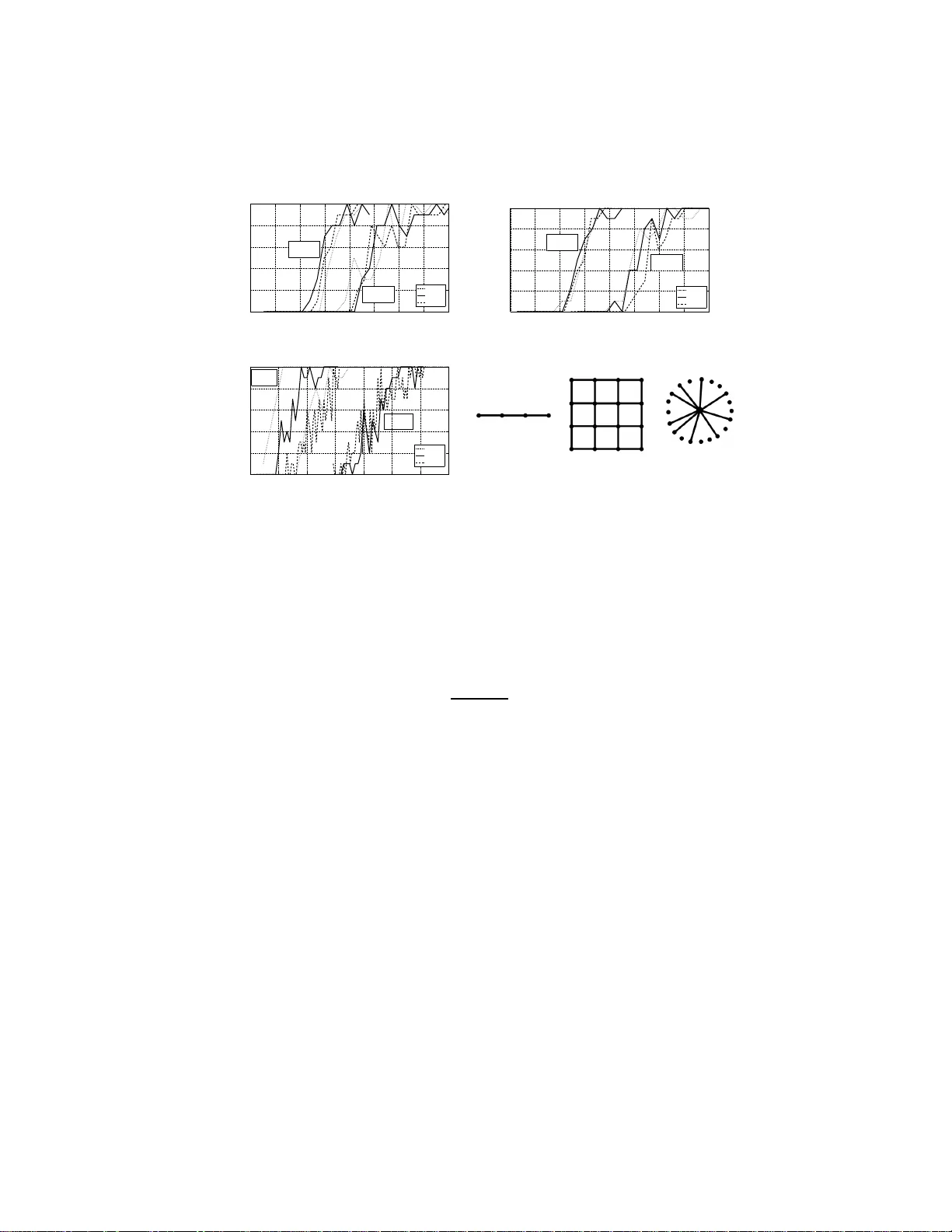
On Learning Discrete Graphic al Models Using Greedy Methods Ali Jalali ECE, Univ ersity of T exas a t Austin alij@mail. utexas.ed u Chris Johnson CS, Unive rsity of T e xas at Austin cjohnson@c s.utexas. edu Pradeep Ra vikumar CS, Unive rsity of T e xas at Austin pradeepr@c s.utexas. edu July 29, 2018 Abstract In this paper , we address the problem of learning the structure of a pairwise graphical model from samples in a high-dimensional setting. Our first main re- sult studies the sparsistency , or consistency in sp arsity pattern recov ery , pro perties of a forward-backwa rd greedy algorithm as applied to general statistical models. As a special case , we then app ly this algorithm to learn the structure of a discrete graphical model via n eighborhoo d estimati on. As a coro llary of ou r general res ult, we deri ve su fficient conditions on the number of samp les n , the maximum n ode- degree d and the pro blem size p , as well as other conditions on the model param- eters, so that the algorithm reco v ers all the edges w ith high probability . Our result guarantees graph selection for samples scaling as n = Ω( d 2 log( p )) , in contrast to e xisting con ve x-optimization based algo rithms that require a sample comple xity of Ω( d 3 log( p )) . Further , the greedy algorithm only requires a restricted strong con vex ity condition which is typically milder than irrepresentability assumptions. W e corroborate these results using numerical simulations at the end. 1 Introd uction Undirected gr aphical m odels, also k nown as Markov r andom fields, a re u sed in a va- riety o f do mains, includin g statistical ph ysics, natur al lan guage p rocessing and ima ge analysis amon g others. In this pap er we are con cerned with the task o f estimating the g raph structur e G of a Markov rando m field (MRF) over a d iscrete rando m vec- tor X = ( X 1 , X 2 , . . . , X p ) , given n independ ent and iden tically distributed samples 1 { x (1) , x (2) , . . . , x ( n ) } . This underly ing gr aph structure enco des condition al indepen- dence assumption s among subsets of the variables, and thus plays an imp ortant role in a broad range of applications of MRFs. Existing appr oa ches: Neighborho od Estimation, Greedy Local Sear ch. Meth ods for estimating such gr aph struc ture inclu de those based on co nstraint an d h ypothe sis test- ing [22], and those that estimate restricted classes of graph structures such as trees [8], polytrees [11], and hyper trees [ 23]. A recent class of successful approach es for graph- ical model structure learning are based on estimating the local neighb orhoo d of each node. One subc lass of these for th e sp ecial c ase o f bo unded degree graphs inv o lve the use of exhaustive search so that their c omputatio nal comp lexity gr ows at least as q uickly as O ( p d ) , where d is th e maximum neighbo rhood size in the graphical model [1, 4, 9]. Another subclass use convex p rogra ms to learn th e n eighbor hood structure: f or instanc e [20, 17, 1 6] estimate the neig hborh ood set for e ach v ertex r ∈ V by op timizing its ℓ 1 -regularized condition al likelihood; [15, 1 0] use ℓ 1 /ℓ 2 -regularized condition al likelihood. Even these method s, however n eed to solve regular ized con- vex pr ograms with typ ically po lynom ial com putation al cost of O ( p 4 ) or O ( p 6 ) , are still expensiv e fo r large prob lems. Ano ther p opular class of app roaches are b ased on using a score metric and searching for the best scoring structure fro m a candida te set of graph struc tures. Exact search is ty pically NP-hard [ 7]; indeed f or gener al discrete MRFs, n ot only is the search spa ce intractab ly large, but calculation of typ ical score metrics itself is co mputatio nally intractable since they in volve computing the partition function associated with the Markov rand om field [26]. Such methods thus h av e to use approx imations and search heuristics for tr actable comp utation. Question: C an on e use lo cal p rocedu res that a re a s ine xpensive as th e heuristic greedy approaches, and yet come with the strong statistical guaran tees of the regularized con vex pr ogram based approa ches? High-dimen sional Estimation; Greedy Methods. Th ere has been an increasin g focu s in recent yea rs on high -dimension al statistical models where the n umber of p arameters p is comp arable to or even larger than the numbe r of observations n . It is n ow well understoo d tha t con sistent estimation is possible even u nder such high-d imensional scaling if some low-dimensional stru cture is impo sed on th e mod el space. Of rele- vance to gr aphical model structure learning is the structu re of sparsity , wh ere a spa rse set of no n-zero parameter s entail a sparse set of edges. A surge o f recent work [5, 12] has shown that ℓ 1 -regularization fo r learnin g such sparse m odels can lead to p ractical algorithm s with strong theo retical g uarantee s. A line of rec ent work ( cf. p aragrap h above) has thus le verag ed this sparsity inducing nature of ℓ 1 -regularization , to propose and analyze conv ex pro grams based on regularized log-likelihood functions. A related line of recen t w o rk on learnin g s parse models h as focused on “stagewise” greed y algo - rithms. Th ese perfo rm sim ple forward steps (ad ding parameter s g reedily), and po ssibly also backward steps (removing parameters greed ily), and y et provide strong statistical guaran tees for th e estimate after a fin ite nu mber o f gree dy steps. The f orward greedy variant which performs just the forward step has app eared in various g uises in multiple commun ities: in mach ine learnin g as bo osting [1 3], in fu nction ap proxim ation [24], and in signal processing as basis pursuit [6]. I n the context of statis tical model estima- tion, Zhang [28] an alyzed the fo rward greedy algo rithm for the ca se of sparse linear regression; and showed that th e forward greedy algorithm is sparsistent (consistent for 2 model selection recovery) un der the same “irrep resentable” conditio n as that r equired for “sparsistency” of the L asso. Zhang [2 7] analyzes a m ore gener al greedy algorith m for sparse linear regression th at perfo rms for ward and bac kward steps, and showed that it is sparsistent un der a weaker restricted eigen value co ndition. Here we ask the question: Can we pr ovide a n analysis of a general fo rwar d ba ckwar d a lgorithm for parameter estimation in general statistical m odels? Specifically , we need to extend the sparsistency an alysis of [2 8] to general no n-linear models, wh ich requires a sub tler analysis due to th e circular req uirement of requirin g to control the thir d order terms in the T a ylor series expansion of the log-likelihoo d, that in turn requires the estimate to be well-behaved. Such extension s in the case of ℓ 1 -regularization occur for in stance in [20, 25, 3]. Our Contributions. In this pap er , we ad dress both q uestions above. In the first pa rt, we analyze the forward backward gre edy algorithm [28] for general s tatistical models. W e n ote that ev en tho ugh we consider th e g eneral statistical model case, our an alysis is much simpler and accessible than [28], and would be o f use e ven to a reader in terested in just the linear mod el case o f Zhan g [28]. In the second part, we u se this to show that when com bined with n eighbo rhoo d estimation, the fo rward backward variant ap- plied to lo cal conditiona l log-likelihoo ds p rovides a simple compu tationally tractable method that adds and deletes edges, but comes with stron g sparsistency guarantees. W e r eiterate that the our first result o n the sparsistency of the f orward backward greedy algorithm for g eneral objec tiv e s is o f inde penden t interest even outside the c ontext o f graphica l mo dels. As we show , the g reedy method is better than the ℓ 1 -regularized counterp art in [20] theoretically , as well as experimen tally . Th e suf ficien t condition on the parameters imposed b y the greedy algorithm is a restricted strong con vexity co ndi- tion [19], which is weaker than the irrepresentable condition required by [20]. Furth er , the num ber of samp les required fo r sparsistent g raph recovery scales as O ( d 2 log p ) , where d is the maximum node degree, in contrast to O ( d 3 log p ) for the ℓ 1 -regularized counterp art. W e cor robo rate th is in our simu lations, w here we find that th e g reedy algorithm requires fewer o bservations than [ 20] for sparsistent graph recovery . 2 Re view , Setup and Notation 2.1 Marko v Random Fields Let X = ( X 1 , . . . , X p ) be a rando m vector, each variable X i taking values in a dis- crete set X of cardinality m . L et G = ( V , E ) d enote a graph with p nodes, c or- respond ing to the p variables { X 1 , . . . , X p } . A p airwise Markov ran dom field over X = ( X 1 , . . . , X p ) is then specified by nod ewise and pairwise fun ctions θ r : X 7→ R for all r ∈ V , and θ r t : X × X 7→ R for all ( r, t ) ∈ E : P ( x ) ∝ exp  X r ∈ V θ r ( x r ) + X ( r,t ) ∈ E θ r t ( x r , x t )  . (1) In this paper, w e largely focu s on the case wher e the variables are binar y with X = {− 1 , +1 } , where we can rewrite (1) to the Ising model fo rm [14] for some set of parameters { θ r } an d { θ r t } as P ( x ) ∝ exp  X r ∈ V θ r x r + X ( r,t ) ∈ E θ r t x r x t  . (2) 3 2.2 Graphical Model Selection Let D := { x (1) , . . . , x ( n ) } deno te the set of n samples, where each p -dim ensional vector x ( i ) ∈ { 1 , . . . , m } p is d rawn i.i.d . from a distribution P θ ∗ of the for m (1), for parameters θ ∗ and graph G = ( V , E ∗ ) over the p variables. Note that the true ed ge set E ∗ can also be expressed as a function of the parameters as E ∗ = { ( r , t ) ∈ V × V : θ ∗ st 6 = 0 } . (3) The graphica l model selection task consists of inferrin g this edge set E ∗ from th e samples D . The goal is to construct an estimator ˆ E n for wh ich P [ ˆ E n = E ∗ ] → 1 as n → ∞ . Denote by N ∗ ( r ) the set of neig hbor s of a vertex r ∈ V , so that N ∗ ( r ) = { t : ( r, t ) ∈ E ∗ } . Then the g raphical mod el selection prob lem is equ iv alent to th at of estimating the neighb orhoo ds ˆ N n ( r ) ⊂ V , so that P [ ˆ N n ( r ) = N ∗ ( r ); ∀ r ∈ V ] → 1 as n → ∞ . For any pair of ra ndom variables X r and X t , the par ameter θ r t fully cha racterizes whether there is an edge b etween them , an d can be estimated via its condition al like- lihood. In par ticular, defining Θ r := ( θ r 1 , . . . , θ r p ) , ou r goal is to use the con ditional likelihood of X r condition ed on X V \ r to estimate Θ r and hence its neighb orhoo d N ( r ) . This condition al distribution of X r condition ed on X V \ r generated by (2) is giv en by the logistic model P  X r = x r    X V \ r = x V \ r  = exp( θ r x r + P t ∈ V \ r θ r t x r x t ) 1 + exp( θ r + P r ∈ V \ r θ r t x r ) . Giv e n the n samples D , the cor respond ing co nditiona l log -likelihood is gi ven by L (Θ r ; D ) = 1 n n X i =1    log   1 + exp   θ r x ( i ) + X t ∈ V \ r θ r t x ( i ) r x ( i ) t     − θ r x ( i ) r − X t ∈ V \ r θ r t x ( i ) r x ( i ) t    . (4) In Sectio n 4 , we stu dy a g reedy alg orithm ( Algorithm 2) that finds th ese node neig h- borho ods ˆ N n ( r ) = Sup p ( b Θ r ) o f each r andom variable X r separately by a greedy stagewise op timization of the c ondition al log-likeliho od of X r condition ed on X V \ r . The algo rithm then co mbines the se neighb orhoo ds to o btain a grap h estimate b E using an “OR” rule: b E n = ∪ r { ( r , t ) : t ∈ ˆ N n ( r ) } . Other rules such as the “ AND” rule, that add an edge only if it occurs in each of the respec ti ve no de n eighbo rhoo ds, co uld be used to co mbine the nod e-neigh borh oods to a grap h estimate. W e show in Theor em 2 that the n eighbo rhood selectio n by the gre edy alg orithm succe eds in re covering th e exact no de-neig hborh oods with high p robab ility , so that by a union b ound, the graph estimates using eithe r the AND o r OR rules would be exact with high pro bability as well. Before we d escribe this greedy algorithm an d its analysis in Section 4 h owe ver, we first con sider the gener al statistical mod el case in th e next section. W e first d escribe the f orward back ward greed y algorithm of Zhang [28] as app lied to g eneral statistical models, followed by a spar sistency analy sis f or this gener al case. W e then spe cialize these gener al results in Section 4 to the gra phical model case. The next section is thu s of indepen dent in terest e ven outside the context of gr aphical models. 4 Algorithm 1 Greedy forward-b ackward algorithm for finding a sparse optimizer of L ( · ) Input : Data D := { x (1) , . . . , x ( n ) } , S topping Threshold ǫ S , Backward Step Factor ν ∈ (0 , 1) Output : Sparse optimizer b θ b θ (0) ← − 0 and b S (0) ← − φ and k ← − 1 while true do { F orwar d Step } ( j ∗ , α ∗ ) ← − a rg min j ∈ ( b S ( k − 1) ) c ; α L ( b θ ( k − 1) + αe j ; D ) b S ( k ) ← − b S ( k − 1) ∪ { j ∗ } δ ( k ) f ← − L ( b θ ( k − 1) ; D ) − L ( b θ ( k − 1) + α ∗ e j ∗ ; D ) if δ ( k ) f ≤ ǫ S then break end if b θ ( k ) ← − arg min θ L  θ b S ( k ) ; D  k ← − k + 1 while true do { Backwa r d Step } j ∗ ← − arg min j ∈ b S ( k − 1) L ( b θ ( k − 1) − b θ ( k − 1) j e j ; D ) if L  b θ ( k − 1) − b θ ( k − 1) j ∗ e j ∗ ; D  − L  b θ ( k − 1) ; D  > ν δ ( k ) f then break end if b S ( k − 1) ← − b S ( k ) − { j ∗ } b θ ( k − 1) ← − arg min θ L  θ b S ( k − 1) ; D  k ← − k − 1 end while end while 3 Gr eedy Algorithm f or General Los ses Consider a random v ar iable Z with distribution P , and l et Z n 1 := { Z 1 , . . . , Z n } d enote n ob servations d rawn i.i.d. acco rding to P . Suppose w e are interested in estimating some parameter θ ∗ ∈ R p of the distribution P that is sparse; denote its num ber of non- zeroes by s ∗ := k θ ∗ k 0 . Let L : R p × Z n 7→ R b e some loss fun ction that assigns a cost to any p arameter θ ∈ R p , for a gi ven set of observations Z n 1 . For ease o f notation, in the sequel, we adopt the shorthand L ( θ ) for L ( θ ; Z n 1 ) . W e assume that θ ∗ satisfies E Z [ ∇L ( θ ∗ )] = 0 . W e now consider the f orward ba ckward greedy algo rithm in Algo rithm 1 that rewrites the algorith m in [2 7] to a llow for gen eral loss f unction s. The a lgorithm starts with an em pty set of active variables b S (0) and gradu ally adds (and r emoves) v airables 5 to the active set until it meets the stopp ing criterion. T his algorithm h as two major steps: the for ward step and the backward step. In the for ward step, the algorithm finds the best next cand idate and adds it to the acti ve set as lon g as it improves the loss func- tion at least by ǫ S , otherwise the stopp ing criterion is met an d the algorithm terminates. Then, in the back ward step, the algorithm checks the influen ce of all variables in the presence of the new added variable. If on e or some of th e previously added variables do not con tribute at least ν ǫ S to the loss fun ction, then the algor ithm removes them from the acti ve set. This procedure ensures that at each round, the loss functio n is im proved by at least (1 − ν ) ǫ S and hence it terminates within a finite number of steps. W e state the assumption s on the loss function so that sparsistency could be guar- anteed. Let us first r ecall th e de finition of restricted strong con vexity from Negah ban et al. [18]. Specifically , for a gi ven set S , the loss fun ction is said to satisfy restricted strong con vexity (RSC) with param eter κ l if L ( θ + ∆; Z n 1 ) − L ( θ ; Z n 1 ) − h∇L ( θ ; Z n 1 ) , ∆ i ≥ κ l 2 k ∆ k 2 2 for all ∆ ∈ S . (5) W e can no w define sp arsity restricted strong con vexity as follows. Specifically , we say that the loss fun ction L satisfies R S C ( k ) with parameter κ l if it satisfies RSC with parameter κ l for all sets S ⊆ { 1 , . . . , p } s uch that k S k 0 ≤ k . In c ontrast, we say the loss f unction satisfies restricted stron g smooth ness (RSS) with parameter κ u , for a given set S if L ( θ + ∆; Z n 1 ) − L ( θ ; Z n 1 ) − h∇L ( θ ; Z n 1 ) , ∆ i ≤ κ u 2 k ∆ k 2 2 for all ∆ ∈ S . W e can d efine RS S ( k ) similarly: the loss function L satisfies RS S ( k ) with para meter κ u if it satisfies R SS with param eter κ u for all sets S ⊆ { 1 , . . . , p } such that k S k 0 ≤ k at all points θ with k θ k 0 ≤ k . Giv en any constants κ l and κ u , and a sample based loss function L , we can typically use concentr ation based argumen ts to o btain bound s on the sample size required so that the RS S and RS C conditions hold with high probab ility . Another prop erty of the loss fu nction th at we require is an up per b ound λ n on the ℓ ∞ norm of the g radient of the loss at the true p arameter θ ∗ , i.e., λ n ≥ k∇L ( θ ∗ ) k ∞ . This captur es the “n oise level” o f the samples with r espect to th e lo ss. Here too, we can typically use co ncentratio n argumen ts to show for instance that λ n ≤ c n (log( p ) /n ) 1 / 2 , for some constant c n > 0 with high probability . Theorem 1 (Sparsistency) . Supp ose the loss function L ( · ) satisfie s RS C ( η s ∗ ) a nd RS S ( η s ∗ ) with p arameters κ l and κ u for some η ≥ 2 + 4 ρ 2 ( p ( ρ 2 − ρ ) /s ∗ + √ 2) 2 with ρ = κ u /κ l . Mor eover , s uppose that the true parameter s θ ∗ satisfy min j ∈ S ∗ | θ ∗ j | > p 32 ρǫ S /κ l . Then if we run Algorithm 1 with st opping th r esho ld ǫ S ≥ (8 ρη / κ l ) s ∗ λ 2 n , the output b θ with suppo rt b S satisfies: (a) Error Bound: k b θ − θ ∗ k 2 ≤ 2 κ l √ s ∗ ( λ n √ η + √ ǫ S √ 2 κ u ) . (b) No False Exclusions: S ∗ − b S = ∅ . (c) No False Inclusions: b S − S ∗ = ∅ . 6 Pr oof. Th e proo f theor em hing es on three m ain le mmas: Lemma s 5 an d 7 are simple consequen ces of the forward and b ackward steps failing when the greedy algorith m stops, and Lemma 6 which uses these two lemmas and extends tech niques from [21] and [19] to obtain an ℓ 2 error bound o n the erro r . Provid ed these lemmas hold, we then show below that the greed y algorithm is spar sistent. However , these lemmas req uire apriori that the RSC and RSS cond itions hold for sparsity size | S ∗ ∪ b S | . Thus, we use the result in Lem ma 8 th at if R S C ( η s ∗ ) holds, then the solution when th e algorithm terminates satisfies | b S | ≤ ( η − 1) s ∗ , an d h ence | b S ∪ S ∗ | ≤ η s ∗ . Thus, we can then apply Lemmas 5, 7 and Lemma 6 to complete the proof as detailed below . (a) Th e result follo ws directly from Lem ma 6, and notin g that | b S ∪ S ∗ | ≤ η s ∗ . In that Lemma, we sho w that the u pper bou nd holds by d rawing f rom fixed po int techniqu es in [21] and [19], and by u sing a simple consequen ce of the forward step failing when the greedy algorithm stops. (b) Following th e argu ment in [27], we use the chain ing argument. For any τ ∈ R , we hav e τ | { j ∈ S ∗ − b S : | θ ∗ j | 2 > τ }| ≤ k θ ∗ S ∗ − b S k 2 2 ≤ k θ ∗ − b θ k 2 2 ≤ 8 η s ∗ λ 2 n κ 2 l + 16 κ u ǫ S κ 2 l | S ∗ − b S | , where the last ineq uality follows from part (a) and th e inequ ality ( a + b ) 2 ≤ 2 a 2 + 2 b 2 . Now , setting τ = 32 κ u ǫ S κ 2 l , and dividing bo th sides by τ / 2 we get 2 |{ j ∈ S ∗ − b S : | θ ∗ j | 2 > τ }| ≤ η s ∗ λ 2 n 2 κ u ǫ S + | S ∗ − b S | . Substituting |{ j ∈ S ∗ − b S : | θ ∗ j | 2 > τ }| = | S ∗ − b S | − |{ j ∈ S ∗ − b S : | θ ∗ j | 2 ≤ τ }| , we get | S ∗ − b S | ≤ |{ j ∈ S ∗ − b S : | θ ∗ j | 2 ≤ τ }| + η s ∗ λ 2 n 2 κ u ǫ S ≤ |{ j ∈ S ∗ − b S : | θ ∗ j | 2 ≤ τ }| + 1 / 2 , due to the setting of the stopping threshold ǫ S . This in turn entails that | S ∗ − b S | ≤ |{ j ∈ S ∗ − b S : | θ ∗ j | 2 ≤ τ }| = 0 , by our assumption on the size of the minimum entry of θ ∗ . (c) Fro m Lemma 7, which provid es a simple consequ ence of the back ward step fail- ing when the greedy alg orithm stops, for b ∆ = b θ − θ ∗ , we h ave ǫ S /κ u | b S − S ∗ | ≤ k b ∆ b S − S ∗ k 2 2 ≤ k b ∆ k 2 2 , so that u sing Lemm a 6 and that | S ∗ − b S | = 0 , we ob tain that | b S − S ∗ | ≤ 4 ηs ∗ λ 2 n κ u ǫ S κ 2 l ≤ 1 / 2 , du e to the setting of the stopping threshold ǫ S . 3.1 Lemmas f or Theor em 1 W e list the simple lemmas that characterize the solutio n ob tained when th e algor ithm terminates, and on which the proof of Theorem 1 hinges. 7 Algorithm 2 Gree dy forw ard-backw ard algorithm for pairwise discrete graph ical model learn- ing Input : Data D := { x (1) , . . . , x ( n ) } , S topping Threshold ǫ S , Backward Step Factor ν ∈ (0 , 1) Output : Estimated Edges b E for r ∈ V do Run Algorithm 1 with L ( · ) described by (4) to get Θ r and its support c N r end for Output b E = S r n ( r, t ) : t ∈ c N r o Lemma 1 (Stopping Forward Step) . Wh en the algorith m 1 stops with parameter b θ supported on b S , we have    L  b θ  − L ( θ ∗ )    < q 2 | S ∗ − b S | κ u ǫ S    b θ − θ ∗    2 . Lemma 2 (Stopp ing Backward Step) . Wh en the algorith m 1 stops with parameter b θ supported on b S , we have    b ∆ b S − S ∗    2 2 ≥ ǫ S κ u    b S − S ∗    . Lemma 3 (Stopping Error Bo und) . When the algo rithm 1 stop s w ith parameter b θ sup- ported on b S , we have    b θ − θ ∗    2 ≤ 2 κ l λ n r    S ∗ ∪ b S    + r 2    S ∗ − b S    κ u ǫ S ! . Lemma 4 (Stopp ing Size) . I f ǫ S > λ 2 n κ u  q 2 η − 1 − q 2 η  − 2 and RS C ( η s ∗ ) hold s fo r some η ≥ 2 + 4 ρ 2  q ρ 2 − ρ s ∗ + √ 2  2 , then the algorithm 1 stops with k ≤ ( η − 1 ) s ∗ . Notice th at if ǫ S ≥ (8 ρη /κ l ) ( η 2 / (4 ρ 2 )) λ 2 n , then , th e assum ption of this lemm a is satisfied. Hence for large value of s ∗ ≥ 8 ρ 2 > η 2 / (4 ρ 2 ) , it suffices to h av e ǫ S ≥ (8 ρη /κ l ) s ∗ λ 2 n . 4 Gr eedy Algorithm f or Pairwise Graphical Models Suppose we are given set of n i.i.d. samp les D := { x (1) , . . . , x ( n ) } , drawn fr om a pairwise Ising model a s in (2), with parameter s θ ∗ , an d grap h G = ( V , E ∗ ) . It will be useful to denote the maximum n ode-d egree in the gr aph E ∗ by d . As we will sho w , our model selection p erform ance depen ds critically on this pa rameter d . W e then prop ose the Algorithm 2 for estimating the underlyin g g raphica l model from the n s amples D . 8 Theorem 2 (Pairwise Spa rsistency) . S uppose we run Algorithm 2 with stop ping thr e sh- old ǫ S ≥ c 1 d log p n , wher e, d is the maximum no de degr ee in the graphical mo del, an d the true parameters θ ∗ satisfy c 3 √ d > min j ∈ S ∗ | θ ∗ j | > c 2 √ ǫ S , an d further that n umber of samples scales as n > c 4 d 2 log p, for some con stants c 1 , c 2 , c 3 , c 4 . Then , with pr o bability at least 1 − c ′ exp( − c ′′ n ) , the output b θ suppo rted on b S satisfies: (a) No False Exclusions: E ∗ − b E = ∅ . (b) No False Inclusions: b E − E ∗ = ∅ . Pr oof. Th is theorem is a corollary to our g eneral Theor em 1 . W e first show th at the condition s of Th eorem 1 hold under the assumptions in this corollary . RSC, R SS. W e first note that the co ndition al log-likelihoo d loss function in (4) c orre- sponds to a logistic likelihood. Moreover , the cov a riates are all binary , an d bounded , and h ence also sub- Gaussian. [19, 2] analyze the RSC and RSS proper ties of gen- eralized lin ear models, of which lo gistic m odels are an instance, a nd show that the following result ho lds if th e covariates are sub-Gaussian. Let ∂ L (∆; θ ∗ ) = L ( θ ∗ + ∆) − L ( θ ∗ ) − h∇L ( θ ∗ ) , ∆ i be the seco nd order T ay lor series remain der . The n, P ropo- sition 2 in [19] states that that there e x ist constants κ l 1 and κ l 2 , independent of n, p such that with probability at least 1 − c 1 exp( − c 2 n ) , for some constants c 1 , c 2 > 0 , ∂ L (∆; θ ∗ ) ≥ κ l 1 k ∆ k 2 ( k ∆ k 2 − κ l 2 r log( p ) n k ∆ k 1 ) for all ∆ : k ∆ k 2 ≤ 1 . Thus, if k ∆ k 0 ≤ k := η d , t hen k ∆ k 1 ≤ √ k k ∆ k 2 , so that ∂ L (∆; θ ∗ ) ≥ k ∆ k 2 2 κ l 1 − κ l 2 r k log p n ! ≥ κ l 1 2 k ∆ k 2 2 , if n > 4( κ l 2 /κ l 1 ) 2 η d log( p ) . In other words, with pro bability at least 1 − c 1 exp( − c 2 n ) , the loss fun ction L satisfies R S C ( k ) with parameter κ l 1 provided n > 4( κ l 2 /κ l 1 ) 2 η d log( p ) . Similarly , it f ollows from [19, 2] th at ther e exist constants κ u 1 and κ u 2 such that with probab ility a t least 1 − c ′ 1 exp( − c ′ 2 n ) , ∂ L (∆; θ ∗ ) ≤ κ u 1 k ∆ k 2 {k ∆ k 2 − κ u 2 k ∆ k 1 } for all ∆ : k ∆ k 2 ≤ 1 , so that by a similar argument, with proba bility at least 1 − c ′ 1 exp( − c ′ 2 n ) , the loss function L satisfies R S S ( k ) with parameter κ u 1 provided n > 4( κ u 2 /κ u 1 ) 2 η d log ( p ) . Noise Level. Next, we obtain a bound o n the n oiselevel λ n ≥ k∇L ( θ ∗ ) k ∞ following similar argumen ts to [20]. L et W denote the gra dient ∇L ( θ ∗ ) of the loss function (4). Any entr y of W has the form W t = 1 n P n i =1 Z ( i ) r t , where Z ( i ) r t = x ( i ) t ( x ( i ) r − P ( x r = 1 | x ( i ) \ s )) are zero-mean , i.i.d. and bound ed | Z ( i ) r t | ≤ 1 . Thus, a n applicatio n of Hoeffd- ing’ s inequality yields that P [ | W t | > δ ] ≤ 2 exp( − 2 nδ 2 ) . Applyin g a u nion b ound 9 over indices in W , we get P [ k W k ∞ > δ ] ≤ 2 exp( − 2 nδ 2 + log( p )) . Thus, if λ n = (log( p ) /n ) 1 / 2 , then k W k ∞ ≤ λ n with prob ability at lea st 1 − ex p( − nλ 2 n + lo g( p )) . W e can no w verify that under the assum ptions in the cor ollary , the con ditions on the stopping size ǫ S and the minimu m absolute value of th e no n-zero param eters min j ∈ S ∗ | θ ∗ j | are satisfied. Mo reover , f rom th e d iscussion above, u nder the sample size scaling in the co rollary , the req uired R S C an d R S S cond itions hold as well. Th us, Theorem 1 yields th at each node neigh borh ood is recovered with no false exclu sions or inclusions with pr obability at least 1 − c ′ exp( − c ′′ n ) . An application of a union bou nd over a ll nodes completes the proof. Remarks. The sufficient condition on the p arameters impo sed by th e greedy al- gorithm is a r estricted strong co n vexity co ndition [19], which is weaker than the ir- representab le condition require d by [ 20]. Fu rther, the n umber of samp les requir ed for sparsistent g raph recovery scales as O ( d 2 log p ) , where d is the maximu m node degree, in contrast to O ( d 3 log p ) fo r the ℓ 1 regularized cou nterpart. W e corro borate this in our simulations, wh ere we find that the gre edy algorith m requires fewer observations than [20] for sparsistent graph recovery . W e also n ote th at the resu lt can also be exten ded to th e g eneral pa irwise gr aphical model case, where each ran dom variable takes values in th e ran ge { 1 , . . . , m } . In that case, the condition al likelihood of each n ode cond itioned on the rest of th e no des takes the form of a multiclass log istic model, and the greedy algorith m would take the form of a “gro up” forward -backward g reedy algo rithm, which w o uld ad d or r emove all the parameters corr espondin g to an edge as a g roup. O ur analysis howev e r n aturally extends to such a group greedy setting as well. The analysis fo r RSC and RSS remains the same and for bo unds on λ n , see equa tion (12) in [1 5]. W e defe r further discussion on this due to the lack of space. 5 Experimental Results W e now present experimental results that illustrate the power of Algor ithm 2 and sup- port our th eoretical guaran tees. W e simulated structure learning o f sev eral different graph structures an d c ompare d the lear ning ra tes o f o ur me thod ag ainst tha t of a stan - dard ℓ 1 -logistic regression method as outlined in [20]. W e performed experiments using 3 different grap h structur es: (a) chain (lin e gr aph), (b) 4-nearest neighb or (g rid g raph) and (c) star gra ph. For each experime nt, we as- sumed a p airwise bina ry Ising mo del in which each θ ∗ r t = ± 1 random ly . For ea ch graph type, we generated a set of n sam ples x (1) , ..., x ( n ) using Gibbs sampling. W e then attempted to lear n the structure of the mod el using both Algorithm 2 as well as ℓ 1 -logistic regression. W e then compa red the actual grap h structure with the em pir- ically learn ed g raph structure s. If the graph structur es matched com pletely then we declared th e result a success oth erwise we declared the result a fa ilur e . W e compared these results over a range of sample sizes ( n ) and averaged the results for each sam ple size over a batch of size 10 . For all g reedy experiments we set the stopping thre shold ǫ S = c log( np ) n , whe re c is a tuning constant, as suggested by Theorem 2, and set the 10 0 0.5 1 1.5 2 2.5 3 3.5 4 0 0.2 0.4 0.6 0.8 1 Control Parameter Probability of Success p = 36 p = 64 p = 100 Greedy Algorithm Logistic Regression (a) Chain (Line Graph) 0 0.5 1 1.5 2 2.5 3 3.5 4 0 0.2 0.4 0.6 0.8 1 Control Parameter Probability of Success p = 36 p = 64 p = 100 Logistic Regression Greedy Algorithm (b) 4-Nearest Neighbor (Grid Graph) 0 1 2 3 4 5 6 7 0 0.2 0.4 0.6 0.8 1 Control Parameter Probability of Success p = 36 p = 64 p = 100 Greedy Algorithm Logistic Regression (c) Star (d) Chain, 4-Nearest Neighbor and Star Graphs Fig 1: Plots of su ccess prob ability P [ b N ± ( r ) = N ∗ ( r ) , ∀ r ∈ V ] versus th e con trol parameter β ( n, p, d ) = n/ [20 d log( p )] for Ising mode l on (a) c hain ( d = 2) , (b) 4- nearest neig hbor ( d = 4 ) and (c ) Star graph ( d = 0 . 1 p ) . T he cou pling param eters are chosen r andom ly fr om θ ∗ st = ± 0 . 50 f or both gre edy an d ℓ 1 -logistic regression meth- ods. As our theo rem sug gests and these figu res show , the greed y algorithm requires less samples to recover th e exact structure of the graphical model. backwards step thresho ld ν = 0 . 5 . For all ℓ 1 -logistic regression experime nts we set the regularization parameter λ n = c ′ p log( p ) /n , where c ′ is set via cross-validation. Figure 1 shows the results for th e chain ( d = 2) , grid ( d = 4) and star ( d = 0 . 1 p ) graphs using both Algorithm 2 an d ℓ 1 -logistic re gression fo r three different gra ph sizes p ∈ { 36 , 6 4 , 100 } with mixed (rand om sign ) coupling s. For each sample size, we generated a batch of 10 d ifferent g raphical m odels and av e raged the probab ility of success (com plete stru cture learne d) over the ba tch. Each cu rve then repr esents the probab ility o f success versus the con trol parameter β ( n, p, d ) = n/ [20 d log( p )] which increases with the samp le size n . These re sults supp ort our theoretical claims a nd demonstra te the efficiency of the gre edy method in compar ison to nod e-wise logistic regression [20]. 11 Refer ences [1] P . Abbeel, D. K oller, an d A. Y . Ng. L earning factor grap hs in polynomial time and sample complex ity . Jour . Mach. Learning Res. , 7:1743– 1788, 2006. [2] A. Agarwal, S. Negah ban, and M. W ainwright. Conv ergence rates of gradient methods for high-dimension al statist ical reco very . In NIPS , 2010. [3] F . Bach . S elf-concordant analysis for logistic regression. Electro nic Journal of Statistics , 4:384–41 4, 20 10. [4] G. Bresler , E. Mossel, and A. Sly . Reconstruction of mark ov random fi elds from samples: Some easy observ ations and algo rithms. In RA NDOM 2008 . [5] E. Candes and T . T ao. The Dan tzig selecto r: Stati stical estimation when p is much l arger than n . Annals of Statistics , 2006. [6] S. Chen, D. L. Donoho, and M. A. Saunders. Atomic decompos ition by basis pursuit. SIAM J . Sci. Computing , 20(1):33–61, 1998. [7] D. Chick ering. Learning Bayesian networks is NP-complete. Pro ceedings of AI and S tatis- tics , 1995. [8] C. Chow and C. Liu. Approximating discrete probability distributions with dependence trees. IEEE T rans. Info. Theory , 14(3):462–4 67, 196 8. [9] I. Csisz ´ ar and Z. T alata. Consistent estimation of the basic neighborhood structure of Marko v rand om fields. The Annals of Statistics , 34(1):123– 145, 2006. [10] C. D ahinden, M. Kalisch, and P . Buhlman n. Decomposition and model selection for large contingenc y tables. Biometrical Jo urnal , 52(2):233–252 , 201 0. [11] S. Dasgupta. Learning polytrees. In Uncertainty on Artificial Intelli gence , pag es 134– 14, 1999. [12] D. Donoho and M . Elad. Maximal sparsity representation via ℓ 1 minimization. Pr oc. Natl. Acad. Sci. , 100:219 7–2202 , March 2003. [13] J. Friedman, T . Hastie, and R. T ibshirani. Additi ve logistic regression: A statistical view of boosting. Annals of Statistics , 28:337–374 , 200 0. [14] E. Ising. B eitrag zur theorie der ferromagnetismus. Zeitschrift f ¨ ur Physik , 31:253–25 8, 1925. [15] A. Jalali, P . Rav ikumar , V . V asuki, and S. Sangha vi. On learning discrete graph ical models using group-sp arse r egularization. In Inter . Conf. on AI and Statistics (AIST A T S) 14 , 2011 . [16] S.- I. Lee, V . Ganapathi, and D. K oller . Ef ficient structure learning of markov networks using l1-regu larization. In Neural Informa tion Proc essing Systems (NIPS) 19 , 2007 . [17] N. Meinshausen and P . B ¨ uhlmann. High dimensional graphs and variable selection with the lasso. Annals of Statistics , 34(3), 2006. [18] S. Neg ahban, P . Ravikumar , M. J. W ainwright, and B. Y u. A unified framewo rk for high- dimensional analysis of m-estimators with decomp osable regularizers. In Neural Informa- tion Pr ocessing Systems (NIPS) 22 , 2009. 12 [19] S. Neg ahban, P . Ravikumar , M. J. W ainwright, and B. Y u. A unified framewo rk for high- dimensional analysis of m-estimators with decomp osable re gularizers. In Arxiv , 2010. [20] P . Ra vikumar , M. J. W ainwright, and J. Lafferty . High-dimension al ising mo del selection using ℓ 1 -regularized log istic regression. Annals of Statistics , 38(3):1287–13 19. [21] A. J. Rothman, P . J. B ickel, E. Lev ina, and J. Zhu. Sparse permutation in variant co variance estimation. 2:494–515, 2008. [22] P . Spirtes, C. Glymour , and R. Scheines. Causation, prediction and search. MIT Press , 2000. [23] N. Srebro. Max imum likelihood bounded tree-width Mark ov networks . Artificial Intelli- gence , 143(1):123–138, 2003. [24] V . N. T emlyako v . Greedy approximation. Acta Numerica , 17:23 5–409, 2008. [25] S. v an de Geer . High-dimension al generalized linear mod els an d t he l asso. The Ann als of Statistics , 36:614– 645, 2008. [26] D. J. A. W elsh. Complexity: Knots, C olourings, and Counting . LMS Lecture Note Series. Cambridge Uni versity P ress, Cambridge, 1993 . [27] T . Zhang. Adapti ve forward-b ackward greedy algorithm for sparse learning with linear models. In Neural Information Pr ocessing Systems (NIP S) 21 , 2008 . [28] T . Z hang. On the consistency of feature selection using greedy least squares regression. J ournal of Machine Learning Resear ch , 10:555–568, 2009. 13 A A uxiliary Lemmas for T heor em 1 In this section , we prove the Lemm as used in the pro of of Theore m 1. No te that when the algorithm terminates, the forward step f ails to go throug h. This entails that L ( b θ ) − inf j ∈ b S c ,α ∈ R L ( b θ + αe j ) < ǫ S . (6) The next lemma shows that this has the co nsequen ce of upper bound ing the de via- tion in loss between the estimated parameter s b θ and the true param eters θ ∗ . Lemma 5 (Stop ping Forward Step) . When the algo rithm stops with pa rameter b θ sup- ported on b S , we have    L  b θ  − L ( θ ∗ )    < q 2 | S ∗ − b S | κ u ǫ S    b θ − θ ∗    2 . (7) Pr oof. Let b ∆ = θ ∗ − b θ . For any η ∈ R , we have L  b θ + η b ∆ j e j  ≤ L  b θ  + η ∇ j L  b θ  b ∆ j + η 2 κ u 2 b ∆ 2 j . Thus, we can establish −| S ∗ − b S | ǫ S < X j ∈ S ∗ − b S  L  b θ + η b ∆ j e j  − L  b θ   ≤ η  L ( θ ∗ ) − L  b θ   + η 2 κ u 2    b ∆    2 2 . Optimizing the RHS over η , we obtain −| S ∗ − b S | ǫ S < −  L ( θ ∗ ) − L  b θ   2 2 κ u k b ∆ k 2 2 , whence the lemma follows. Lemma 6 (Stop ping Erro r Bound ) . When the algorithm stops with parameter b θ sup- ported on b S , we have k b θ − θ ∗ k 2 ≤ 2 κ l λ n r    S ∗ ∪ b S    + r 2    S ∗ − b S    κ u ǫ S ! . (8) Pr oof. For ∆ ∈ R , let G (∆) = L ( θ ∗ + ∆) − L ( θ ∗ ) − r 2    S ∗ − b S    κ u ǫ S k ∆ k 2 . It can be seen that G (0) = 0 , an d from the previous lemma, G ( b ∆) ≤ 0 . Further, G (∆) is sub-ho mogen eous (over a limited range ): G ( t ∆) ≤ tG (∆) for t ∈ [0 , 1] . Thus, 14 for a carefully chosen r > 0 , if we show th at G (∆) > 0 for all ∆ ∈ { ∆ : k ∆ k 2 ≤ r , k ∆ k 0 ≤ | S |} , where S = | b S ∪ S ∗ | , then it follows th at k b ∆ k 2 ≤ r . If not, th en there would exist some t ∈ [0 , 1 ) such tha t k t b ∆ k = r , whence we would ar rive at th e contradictio n 0 < G ( t b ∆) ≤ tG ( b ∆) ≤ 0 . Thus, it rem ains to show that G (∆) > 0 fo r all ∆ ∈ { ∆ : k ∆ k 2 ≤ r, k ∆ k 0 ≤ | S |} . By restricted strong con vexity proper ty of L , we hav e L ( θ ∗ + ∆) − L ( θ ∗ ) ≥ h∇L ( θ ∗ ) , ∆ i + κ l 2 k ∆ k 2 2 . W e can establish h∇L ( θ ∗ ) , ∆ i ≥ − |h∇L ( θ ∗ ) , ∆ i| ≥ − k∇L ( θ ∗ ) k ∞ k ∆ k 1 = λ n k ∆ k 1 , and hence, G ( θ ∗ + ∆) ≥ − λ n k ∆ k 1 + κ l 2 k ∆ k 2 2 − r 2    S ∗ − b S    κ u ǫ S k ∆ k 2 > k ∆ k 2 κ l 2 k ∆ k 2 − λ n r    S ∗ ∪ b S    − r 2    S ∗ − b S    κ u ǫ S ! > 0 , if k ∆ k 2 = r for r = 2 κ l λ n r    S ∗ ∪ b S    + r 2    S ∗ − b S    κ u ǫ S ! . This conclu des th e proo f of the l emma. Next, we no te that whe n the algorith m terminates, the backward step with the c ur- rent parameter s has failed to go thro ugh. This entails that inf j ∈ b S L ( b θ − b θ j e j ) − L ( b θ ) > ǫ S / 2 . (9) The next lemma sho ws the conseq uence of this bound. Lemma 7 (Stoppin g Backward Step) . When th e alg orithm stops with p arameter b θ supported on b S , we have    b ∆ b S − S ∗    2 2 ≥ ǫ S κ u    b S − S ∗    . (10) 15 Pr oof. W e have | b S − S ∗ | inf j ∈ b S L ( b θ − b θ j e j ) ≤ X j ∈ b S − S ∗ L ( b θ − b θ j e j ) ≤ | b S − S ∗ |L ( b θ ) + X j ∈ b S − S ∗  ∇ j L ( b θ ) b θ j + κ u 2 b θ 2 j  ≤ | b S − S ∗ |L ( b θ ) + κ u 2    b ∆ b S − S ∗    2 2 , where the second ineq uality uses the fact that [ ∇L ( b θ )] b S = 0 . Substituting (9) above, the lemma follows. B Lemmas on the Stopping Size Lemma 8. If ǫ S > λ 2 n κ u 1 2 ρ √ γ − q ρ 2 − ρ k ∗ √ 1+ γ − q 2 2+ γ ! − 2 and RS C ((2 + γ ) k ∗ ) holds for some γ ≥ 4 ρ 2  q ρ 2 − ρ k ∗ + √ 2  2 , then the algorithm stops with k ≤ (1 + γ ) k ∗ . Pr oof. Consid er th e first time the algorithm r eaches k = (1 + γ ) k ∗ + 1 , th en b y Lemma 9 and 11, we hav e r k − 1 − k ∗ k − 1 ≤ s | b S ( k − 1) − S ∗ | | b S ( k − 1) ∪ S ∗ | ≤ 2 κ u p κ u ( κ u − κ l ) κ 2 l q | b S ( k − 1) ∪ S ∗ | + 2 κ u κ l λ n √ κ u ǫ S + s 2 | S ∗ − b S ( k − 1) | | S ∗ ∪ b S ( k − 1) | ! ≤ 2 κ u κ l r  κ u κ l  2 − κ u κ l √ k − 1 + 2 κ u κ l λ n √ κ u ǫ S + r 2 k ∗ k + k ∗ − 1 ! . Hence, we get 1 2 ρ √ γ − q ρ 2 − ρ k ∗ √ 1 + γ − r 2 2 + γ ≤ λ n √ κ u ǫ S . For γ ≥ 4 ρ 2  q ρ 2 − ρ k ∗ + √ 2  2 , the LHS is p ositiv e and we arr iv e to a contradiction with the assumption on ǫ S . When the alg orithm reaches the sup port size of k at the be ginning of the forward step, i.e., we ad ded the k th variable to the support and the backward step did no t remove any variable, let b θ ( k ) denote the cu rrent param eter and b S ( k ) = Supp ( b θ ( k ) ) with k = | b S ( k ) | . Let θ ∗ be the target param eter matrix (i.e., E [ ∇L ( θ ∗ )] = 0 ), with S ∗ = Supp ( θ ∗ ) and k ∗ = | S ∗ | . Lemmas 9, 1 0 and 11 follow along similar lin es to 16 their counter parts in Le mmas 7, 5 an d 6 respectively: the latter h eld when the algo rithm terminates, while the lemm as below hold at any iterate b θ ( k ) where we h av e first ad ded the k th variable to the support. W e provide their detailed proofs for completeness. Lemma 9 ( General Backward Step) . The first time the alg orithm r ea ches a suppo rt size of k > k ∗ +4  κ u κ l  4 +1 a t the beginning of th e forward step, a ssuming RS C  | b S ( k ) ∪ S ∗ |  holds, we have    b θ ( k − 1) b S ( k − 1) − S ∗    2 2 ≥   s | b S ( k − 1) − S ∗ | κ u − 2 κ u √ κ u − κ l κ 2 l   2 δ ( k ) f . (11) Pr oof. Und er the assumption of the lemma, the immed iate p revious backward step has not gone throug h and hence, inf j ∈ b S ( k ) − S ∗ L  b θ ( k ) − b θ ( k ) j e j  − L  b θ ( k )  ≥ δ ( k ) f 2 . Consequently , we get | b S ( k − 1) − S ∗ | δ ( k ) f 2 ≤ X j ∈ b S ( k − 1) − S ∗ L ( b θ ( k ) − b θ ( k ) j e j ) − L ( b θ ( k ) ) ≤ κ u 2    b θ ( k ) b S ( k − 1) − S ∗    2 2 ≤ κ u 2     b θ ( k − 1) b S ( k − 1) − S ∗    2 +    ∆ ( k )    2  2 , where, ∆ ( k ) = b θ ( k ) b S ( k − 1) − b θ ( k − 1) . This entails that   s | b S ( k − 1) − S ∗ | κ u δ ( k ) f −    ∆ ( k )    2   2 ≤    b θ ( k − 1) b S ( k − 1) − S ∗    2 2 . Thus, it suffi ces to show that   ∆ ( k )   2 ≤ 2 κ u κ 2 l q ( κ u − κ l ) δ ( k ) f . From the forward step, we hav e L  b θ ( k − 1)  − inf j / ∈ b S ( k − 1) ,α ∈ R L  b θ ( k − 1) + αe j  = δ ( k ) f . Let ( j ∗ , α ∗ 6 = 0) be the optimizer of the equation above. Now , we have κ l 2    ∆ ( k )    2 2 ≤ L  b θ ( k ) b S ( k − 1)  − L  b θ ( k − 1)  ≤ L  b θ ( k ) b S ( k − 1)  − L  b θ ( k )  + L  b θ ( k )  − L  b θ ( k − 1)  ≤ κ u 2    b θ ( k ) j ∗    2 − κ l 2    ∆ ( k )    2 2 − κ l 2    b θ ( k ) j ∗    2 . 17 Hence,   ∆ ( k )   2 2 ≤ κ u − κ l 2 κ l    b θ ( k ) j ∗    2 and we only need to show that    b θ ( k ) j ∗    ≤ 2 κ u κ l q 2 κ l δ ( k ) f . Since    b θ ( k ) j ∗    ≤    b θ ( k ) j ∗ − α ∗    + | α ∗ | , we can eq uiv alen tly control th e latter two term s. First, by fo rward step co nstruction , κ l 2 | α ∗ | 2 ≤ L  b θ ( k − 1)  − L  b θ ( k − 1) + α ∗ e j ∗  = δ ( k ) f and hen ce | α ∗ | ≤ q 2 κ l δ ( k ) f . Seco nd, we claim that    b θ ( k ) j ∗ − α ∗    ≤ 2 κ u − κ l κ l | α ∗ | and we are done. In contrary , suppose    b θ ( k ) j ∗ − α ∗    2 >  2 κ u − κ l κ l  2 | α ∗ | 2 ≥ κ u κ l | α ∗ | 2 . W e have κ l 2    b θ ( k ) j ∗ − α ∗    2 > κ u 2 | α ∗ | 2 ≥ L  b θ ( k ) − α ∗ e j ∗  − L  b θ ( k )  ≥ L  b θ ( k ) − α ∗ e j ∗  − L  b θ ( k − 1)  + L  b θ ( k − 1)  − L  b θ ( k )  ≥ κ l 2    ∆ ( k )    2 2 + κ l 2    b θ ( k ) j ∗ − α ∗    2 + ∇ j ∗ L  b θ ( k − 1)   b θ ( k ) j ∗ − α ∗  + κ l 2    ∆ ( k )    2 2 + κ l 2    b θ ( k ) j ∗    2 . This is a co ntradictio n provided that κ l 2    b θ ( k ) j ∗    2 + ∇ j ∗ L  b θ ( k − 1)   b θ ( k ) j ∗ − α ∗  ≥ 0 . Later , we will show that Sign  ∇ j ∗ L  b θ ( k − 1)  = − Sign ( α ∗ ) an d κ l | α ∗ | ≤    ∇ j ∗ L  b θ ( k − 1)     ≤ κ u | α ∗ | . W ith these, if b θ ( k ) j ∗ α ∗ ≤ 1 , we have ∇ j ∗ L  b θ ( k − 1)   b θ ( k ) j ∗ − α ∗  ≥ 0 and the claim follows. Otherwise, we hav e    b θ ( k ) j ∗    ≥    b θ ( k ) j ∗    − | α ∗ | =    b θ ( k ) j ∗ − α ∗    so that    b θ ( k ) j ∗    ≥ 2 κ u κ l | α ∗ | and hence, κ l 2    b θ ( k ) j ∗    2 + ∇ j ∗ L  b θ ( k − 1)   b θ ( k ) j ∗ − α ∗  ≥ κ l 2 2 κ u κ l | α ∗ |    b θ ( k ) j ∗ − α ∗    − κ u | α ∗ |    b θ ( k ) j ∗ − α ∗    = 0 . T o get the claimed pro perties of ∇ j ∗ L  b θ ( k − 1)  , note that κ l 2 | α ∗ | 2 ≤ L  b θ ( k − 1)  − L  b θ ( k − 1) + α ∗ e j ∗  ≤ − κ l 2 | α ∗ | 2 − ∇ j ∗ L  b θ ( k − 1)  α ∗ , and hen ce Sign  ∇ j ∗ L  b θ ( k − 1)  = − Sign ( α ∗ ) a nd κ l | α ∗ | ≤    ∇ j ∗ L  b θ ( k − 1)     . Also, we can establish κ u 2 | α ∗ | 2 ≥ L  b θ ( k − 1)  − L  b θ ( k − 1) + α ∗ e j ∗  ≥ − κ u 2 | α ∗ | 2 − ∇ j ∗ L  b θ ( k − 1)  α ∗ . 18 Since −∇ j ∗ L  b θ ( k − 1)  α ∗ ≥ 0 , we can con clude that    ∇ j ∗ L  b θ ( k − 1)     ≤ κ u | α ∗ | . This conclu des th e proo f of the l emma. Lemma 10 ( General Forward Step) . Th e first time th e algo rithm r eaches a sup port size of k at the beginning o f the forwar d step, we hav e    L ( θ ∗ ) − L  b θ ( k − 1)     ≤ r 2    S ∗ − b S ( k − 1)    κ u δ ( k ) f    θ ∗ − b θ ( k − 1)    2 . Pr oof. Und er the assumption of the lemma, we hav e L  b θ ( k − 1)  − inf j / ∈ b S ( k − 1) ,α ∈ R L  b θ ( k − 1) + αe j  = δ ( k ) f . For any η ∈ R , we hav e −    S ∗ − b S ( k − 1)    δ ( k ) f ≤ X j ∈ S ∗ − b S ( k − 1) L  b θ ( k − 1) + η θ ∗ j e j  − L  b θ ( k − 1)  ≤ η X j ∈ S ∗ − b S ( k − 1) ∇ j L  b θ ( k − 1)  θ ∗ j + η 2 κ u 2    θ ∗ − b θ ( k − 1)    2 2 ≤ η  L ( θ ∗ ) − L  b θ ( k − 1)  + η 2 κ u 2    θ ∗ − b θ ( k − 1)    2 2 . Optimizing the RHS over η , we obtain | S ∗ − b S ( k − 1) | δ ( k ) f ≥  L ( θ ∗ ) − L  b θ ( k − 1)  2 2 κ u k θ ∗ − b θ ( k − 1) k 2 2 . This conclu des th e proo f of the l emma. Lemma 11 (G eneral Error Bou nd) . Th e first time the algorithm reaches a support siz e of k at the beginning o f the fo rwar d step, assuming R S C  | b S ( k ) ∪ S ∗ |  holds, we have    b θ ( k − 1) b S ( k − 1) − S ∗    2 2 ≤ 4 κ u | S ∗ ∪ b S ( k − 1) | δ ( k ) f κ 2 l λ n √ κ u ǫ S + s 2 | S ∗ − b S ( k − 1) | | S ∗ ∪ b S ( k − 1) | ! 2 . Pr oof. Let G (∆) := L ( θ ∗ + ∆) − L ( θ ∗ ) − q 2 | S ∗ − b S ( k − 1) | κ u δ ( k ) f k ∆ k 2 . It can b e seen that G (0) = 0 , a nd fr om Lemma 10, G ( b θ ( k − 1) − θ ∗ ) ≤ 0 . Further, G (∆) is sub -hom ogeneo us ( over a limited ran ge): G ( t ∆) ≤ t G (∆) for t ∈ [0 , 1] . Thu s, fo r 19 a ca refully cho sen r > 0 , if we show tha t G (∆) > 0 f or all ∆ ∈ { ∆ : k ∆ k 2 ≤ r , k ∆ k 0 ≤ | S |} , where S = | b S ( k ) ∪ S ∗ | , then it f ollows that k b θ ( k ) − θ ∗ k 2 ≤ r . If not, then there wou ld exist some t ∈ [0 , 1) such that k t ( b θ ( k ) − θ ∗ ) k 2 = r , whenc e we would arri ve at the contradictio n 0 < G  t ( b θ ( k ) − θ ∗ )  ≤ tG  b θ ( k ) − θ ∗  ≤ 0 . Thus, it rem ains to show that G (∆) > 0 fo r all ∆ ∈ { ∆ : k ∆ k 2 ≤ r, k ∆ k 0 ≤ | S |} . By RSC , we have L ( θ ∗ + ∆) − L ( θ ∗ ) ≥ ∇L ( θ ∗ ) · ∆ + κ l 2 k ∆ k 2 2 . W e can establish ∇L ( θ ∗ ) · ∆ ≥ −|∇L ( θ ∗ ) · ∆ | ≥ −k∇L ( θ ∗ ) k ∞ k ∆ k 1 = − λ n k ∆ k 1 , and hence, G ( θ ∗ + ∆) ≥ − λ n k ∆ k 1 + κ l 2 k ∆ k 2 2 − q 2 | S ∗ − b S ( k − 1) | κ u δ ( k ) f k ∆ k 2 ≥ k ∆ k 2  κ l 2 k ∆ k 2 − λ n q | S ∗ ∪ b S ( k ) | − q 2 | S ∗ − b S ( k − 1) | κ u δ ( k ) f  > 0 , if k ∆ k 2 = r for r = 2 κ l  λ n q | S ∗ ∪ b S ( k ) | + q 2 | S ∗ − b S ( k − 1) | κ u δ ( k ) f  . Hence,    b θ ( k − 1) b S ( k − 1) − S ∗    2 2 ≤ 4 κ u | S ∗ ∪ b S ( k − 1) | δ ( k ) f κ 2 l   λ n q κ u δ ( k ) f + s 2 | S ∗ − b S ( k − 1) | | S ∗ ∪ b S ( k − 1) |   2 . Finally , consider the f act that δ ( k ) f ≥ ǫ S . This conclud es the proof of the lemma. 20