The Complexity of Relating Quantum Channels to Master Equations

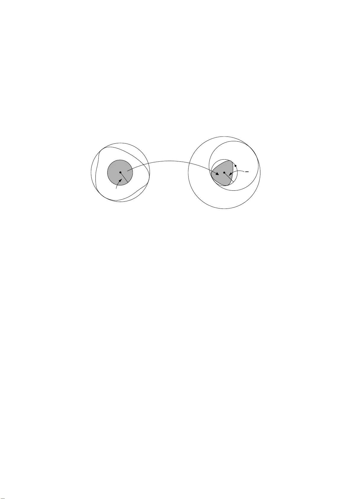
The Complexit y of Relating Quan tum Channels to Master Equations T ob y S. Cubitt ∗ 1,2 , Jens Eisert 3,4 , and Mic hael M. W olf 5,6 1 Dep ar tment of Math ematics, University of Bristol University Walk, Bristol BS8 1TW, UK 2 Dep ar tamento de An´ alisis Matem´ atic o , Universidad Complutense de Madrid Plaza de Ciencias 3, Ciudad Unive rsitaria, 280 40 Madrid, Sp ain 3 Dahlem Center for Complex Quantum Systems F r e ie Universit¨ at Berlin, 14195 Berlin, Germany 4 Institute for Physics and Astr ono my, Potsdam Unive rsity, 14476 Potsdam, Germany 5 Niels Bohr Institute, Ble gdamsvej 17, 2100 Cop enhagen, Denmark 6 Zentrum Mathematik, T e chnische Universit¨ at M ¨ unchen, 85748 Gar ching, Germany Octob er 23, 20 18 Abstract Completely p ositiv e, trace pr eserving (CPT) maps and Lindb lad master equations are b oth widely used to describ e the dyn amics of op en qu an tum sy s tems. The connection b et w een these t w o descrip- tions is a classic topic in mathematical p h ysics. One direction was solv ed b y the no w famo us result due to Lindblad, Kossak o wski Gorini and S udarshan, w h o ga v e a complete c haracterisation of the m aster equations that generate completely p ositiv e semi-groups. Ho w ev er, the other direction h as remained op en: giv en a CPT map, is th ere a Lindblad master equation that generates it (and if so, can we ﬁn d it’s form)? Th is is sometimes kno wn as the Marko vianity pr oblem . Ph ys- ically , it is asking how one can deduce underlyin g physic al p ro cesses from e xp erimen tal obs erv a tions. W e giv e a complexity theoretic answer to this problem: it is NP- hard. W e also giv e an explicit algorithm that reduces th e problem ∗ tcubitt@mat.ucm.es 1 to in teger se mi-deﬁn ite p rogramming, a well- known NP problem. T o- gether, these results imply that resolving the question of w h ic h CPT maps can b e generated by master equations is tan tamoun t to solving P=NP: any eﬃcien tly computable criterion for Marko v ianity w ould imply P=NP; whereas a pro of that P=NP would im p ly that our algo- rithm a lready giv es an eﬃcien tly computable criterion. Thus, unless P do es equal NP , there cannot exist an y simple criterion for determining when a C PT map has a master equation d escription. Ho w ev er, we also sho w that if th e system d imension is ﬁ x ed (rele- v an t for curren t quantum pro cess tomograph y exp erimen ts), then ou r algorithm scales eﬃcien tly in th e required precision, allo wing an u n - derlying Lin dblad master equation to b e determin ed eﬃcien tly from ev en a single snap s hot in this case. Our wo rk also leads to similar complexit y-theoretic answ ers to a related long-standing op en problem in pr ob ab ility theory . Con ten ts 1 In tro duction 3 1.1 The Quan tum Problem . . . . . . . . . . . . . . . . . . . . . . 4 1.2 The Classical Problem . . . . . . . . . . . . . . . . . . . . . . 6 1.3 Implications for Ph ysics . . . . . . . . . . . . . . . . . . . . . 6 1.4 Outline . . . . . . . . . . . . . . . . . . . . . . . . . . . . . . . 8 2 Preliminaries 11 3 The Quan tum Problem 14 3.1 The Computational Marko vianit y Problem . . . . . . . . . . . 14 3.2 The Computational Lindblad Generator Problem . . . . . . . 16 4 NP-hardness 25 4.1 Enco ding 1-in-3SA T . . . . . . . . . . . . . . . . . . . . . . . 25 4.2 P erturbations . . . . . . . . . . . . . . . . . . . . . . . . . . . 32 5 An Algorithm 37 6 The Classical Problem 43 7 Conclusions 45 8 Ac kno wledgemen ts 46 2 1 In tro duction Noise ab ounds in quan tum mec hanical systems, so it’s no surprise that the mathematics o f op en quantum systems p ermeates many areas of quan tum theory . In quan tum information theory , noisy evolution is usually mo delled b y completely p ositiv e, trace preserving (CPT) maps. CPT maps a re o ften referred to as quantum channel s , as they play the same role in quantum information theory a s classical channels (sto chastic maps) play in classical information theory: they g iv e a discrete, blac k-b ox description o f how input states are transformed into output states. Just as in classical information theory , questions r anging from communi- cation capacities to error-correction and fault-t oleran t computation b eneﬁt from abstracting a w a y the underlying phys ics in this w a y [1]. CPT maps also arise naturally in exp erimen tal measuremen t o f quan tum dynamics, when a complete “ snapshot” of t he dynamics is reconstructed via quantum pr o c ess tomo gr aphy [1]. The reconstructed snapshot is a CPT map describing how initial states are transformed b y t he ev olution into states at the time of mea- suremen t. Noisy evolution in other areas of quan tum p hysics , o n the other hand, is usually mo delled b y master equations. Thes e directly describ e the underly- ing phy sical pro cesses go v erning the ev olution, in the f orm of a diﬀeren tial equation fo r the time-ev olution of the densit y matrix. They are frequen tly used to mo del realistic exp erimen tal set-ups, where external noise and dis- sipation must in v ariably b e accoun ted for, esp ecially in quantum optics [2] and condensed-matter phy sics [3]. In describing a noisy evolution by a master equation, there is an implicit assumption that the eﬀect of the external environmen t o n the system’s ev o- lution can b e describ ed in terms of the system’s degrees of freedom alone. Giv en this assumption, the master equation mu st necessarily b e Markovian . One justiﬁcation for this is if the un derlying ph ysical pro cesses are forgetful— as they commonly are to a go o d appro ximation. Con v ersely , if the Mark ovian assumption do esn’t hold, then there is no wa y t o decrib e the ev olution phys - ically without enlarging the system b eing mo delled to include (some of ) the en vironmen t degrees of freedom. Mathematically , a Marko vian master equation g enerates a one-parameter (time t ) semi-group (ev olving for time t a nd then time s is equiv alen t t o ev olving fo r time t + s ) of CPT maps (the evolution m ust b e completely p ositiv e and trace preserving a t a ll times if proba bilities o f measuremen t outcomes are to b e p ositiv e and sum to one). 3 1.1 The Quan tum Problem The connection b etw een these t w o descriptions of op en quantum systems— the blac k-b ox, discrete-time description o f CPT maps, and the con tin uous- time, phy sical description of master equations—is a classic topic in mathe- matical phy sics. Tw o ques tions n aturally arise: given a master equation, do es it generate a a completely po sitiv e ev olution (and if so whic h CPT m aps do es it pro duce)? Con v ersely , giv en o ne or more CPT maps, is there an underly- ing Mark o vian master equation t hat generates them ( and if so whic h one)? These questions can equiv alen tly b e stated more mat hematically: giv en a lin- ear op erator, do es it g enerate a completely p ositiv e semi-group? Con v ersely , giv en one or more CPT maps, are they mem b ers of a completely p ositiv e semi-group? In seminal pap ers from the 197 0’s, Lindblad [4 ], G orini, Ko ssako vski a nd Sudarshan [5] gav e a complete answ er to the ﬁrst question (for ﬁnite dimen- sional s ystems ∗ ). They deriv ed the general form—no w kno wn as the Lindbla d form —for the generators of one-par ameter completely p ositiv e semi-groups. Just as any discrete transformation of quantum states m ust b e completely p ositiv e and t race-preserving if probabilities are to remain p ositiv e and nor- malised for an y input state, a master equation must b e of Lindblad form if it is to b e phy sical, since an ev olution that is no t o f this form will necessarily lead to negative probabilities. † The conv erse question, ho w ev er, has remained op en. F or the case of a single CPT map, w e will refer to the pro blem of deciding whether it is a member of a completely p ositiv e semi-group as the Mark o v ianity pr oblem , since CPT maps that ar e generated b y a Lindblad master e quation are said to b e M arkovia n . ‡ The main result of this w ork is a comple xity -theoretic answ er to the Mark ovianit y pro blem (whic h will b e made more rigorous later): ∗ F or subtleties inv ovled in ﬁnding the most gene r al form of a generator in inﬁnite- dimensional quantum systems, see Ref. [6]. † There exis ts a la rge literature on “ non-Markovian master equatio ns”, which are not of Lindbla d for m. These ca n provide a useful pheno menological descr iption of quantum evolution. But since they necessa rily predict neg ative pro babilities for some physical measurement outco mes, they are only v alid for a r estricted set of “a llowed” initial states. If the system is prepared in a state outside of this allowed set, the non- Ma rko vian master equation beco mes inv alid. ‡ Note that this term is not used consistently thr oughout the literature. Here, we stic k to the standard use of the term Markovian in the mathematical physics liter ature to mean the time-homo gene ous Markovianit y problem, in which the master equation is ass umed to be time-independent. So metimes, in particula r in the con text of condensed-matter ph ysics, master equations a re also re fer red to as being Markovian if they are of Lindblad form, but may b e time-dep endent. O ne co uld also ado pt the established clas sical terminology and call the problem considered in this work the quantum emb e dd ing pr oblem . 4 Theorem 1 The Markovianity pr oblem is NP-har d. Our pro o f easily extends to more general pro blems, suc h a s deciding whether a f amily of CPT maps a re mem b ers of the same completely p ositive semi- group, or computing any “measure” of Marko vianit y [7– 12]. “Hardness” here is in the rigo rous complexit y-theoretic sense, whic h will b e explained mor e precisely b elow. (See also R efs. [13, 14].) It concerns the scaling of computat ional eﬀort as a function of the size of the pro blem, i.e. as a function of the total amoun t of informat ion required to sp ecify the CPT map. But a more reﬁned analysis can break do wn the ov erall pro blem size here in to t w o comp o nen ts: the dimension of the system, a nd the precision to whic h the CPT map is sp eciﬁed. W e will analyse the complexity of the Mark o vianit y problem with resp ect to b oth these parameters, and sho w that the NP-hardness is a consequence of scaling of the dimension. ∗ W e will also sho w—hin ted at already in Ref. [7]—that for a ﬁxe d dimension, the Marko- vianit y problem can b e decided eﬃcien tly in t he precision. Th us, tho ugh the problem in general is (v ery lik ely) in tractable, in practical con texts a rising in current quantum exp erimen ts, where the dimension is in v ariably small, the question of whether a giv en (f amily of ) CPT map(s) is consisten t with Mark o vian dynamics can b e tested eﬃcien tly from ev en a single snapshot in time. W e will giv e an explicit algorithm in this case, along with a careful analysis of its scaling: Theorem 2 F or any ﬁx e d ph ysic al dimension the Markovian ity p r oblem c an b e solve d in a run-time that sc ales p olynomial ly (b oth in the n umb er of digits to which the entries of the CPT map ar e sp e c i ﬁ e d, and the pr e cision to which the answer should b e giv e n). Theorem 1 prov es t hat deciding Mark ov ianity is at least as hard as an y problem in the complexit y class NP . The a lgorithm of Theorem 2 reduces the problem to solving an integer semi-deﬁnite program, a problem that is con tained in t he class NP . T ogether, these results imply tha t: Corollary 3 Finding an eﬃciently c omputable criterion for Markovianity is e quivalent to solving the ( in)famous P = NP question; pr ovin g P = NP would imply the algorithm of The or em 2 is eﬃcie n t, wher e as ﬁndin g an y eﬃciently c omputable criterion for Markovianity would pr ove P = NP. ∗ Note that the re le v an t parameter here is the system dimension, not the num be r o f qubits (the base-2 logarithm of the dimension), as the amo un t of information required to sp ecify the CP T map—the problem size—scales with the (square of ) the dimension. The time required to p erfor m pro ces s tomogr aphy scale s o nly p olyno mially in the dimension, so is eﬃcien t in this co n text. 5 1.2 The Classical Problem The a nalogous questions can equally w ell b e p osed for classi c al dynamics. In fact, the resulting mathematical problems are ev en older and more exten- siv ely studied. The classical analo gue of a CPT map is a sto chastic map, whic h, in t he con text o f information theory , also describ es a classical commu- nication c hannel. The c lassical analogue of a mas ter equation is a con tin uous- time Mark o v c hain, and the Mark o v-c hain ana logue of the Lindblad form can b e found in any go o d text b o ok on Mark ov pro cesse s (see e.g. Ref. [15]). Ho w ev er, the conv ers e question: give n a sto chastic map, can it b e gener- ated by a con tin uous-time Marko v chain, has remained a thorny op en prob- lem in probability theory for ov er 70 y ears! It is kno wn as the emb e ddin g pr oblem for sto c hastic maps, a nd w as ﬁrst p o sed at least as lo ng a go as 1937 b y Elfving [16]. Though it has b een the sub ject of in v estigation o v er the man y interv ening decades [17–19], the general em b edding problem has remained op en [20] until now. Although there is a sense in whic h the classical em b edding problem can b e v iew ed as a sp ecial case of the quan tum Mark o vianit y problem, mathemat- ically t he tw o are inequiv a len t: a result concerning o ne do es not necessarily imply an ything ab out the other. Ho w ev er, it turns out that v ery similar tec h- niques can b e used t o tack le b oth problems, a llo wing us to also show that: Theorem 4 The emb e d d ing pr oblem is NP-har d. This ﬁnally r esolv es the long-standing embedding pro blem, in the sense that no eﬃcien tly computable (p olynomial-time) criterion for embeddabil- it y can exist unless P=NP; the existence o f any suc h eﬃcien tly computable criterion would imply P=NP. Rather than duplicating ev erything for the classical case, we will fo cus in this pap er on t he somewhat mor e complicated quan tum problem, and then p oin t out ho w the r esults can b e adapted to the older classical em b edding problem. A more detailed exp osition of the classical result can b e found in Ref. [21]. 1.3 Implications for Ph ysics The Marko vianit y and em b edding problems are not only of mathematical in- terest. They are a lso crucial problems in ph ysics. What is t he b est p ossible measuremen t data that an exp erimen talist could conceiv ably gather ab out a system’s dynamics? They could, for example, rep eatedly prepare the system in a n y desired initial state, allow it to evolv e for some p erio d of time, and 6 then p erfo rm any desired measuremen t. In fa ct, b y c ho osing tomographi- cally complete bases of initial states and measureme nts , and carrying out this pro cedure only a ﬁnite num ber of times, it is already p o ssible to recon- struct a complete “ snapshot” of the system dynamics at any particular time to arbitrar y accuracy . In the quan tum setting, this is quantum pr o c ess to- mo gr aphy [1], but the general principle ob viously applies equally w ell in the classical setting. Remark ably , thanks to the dramatic progress in exp erimen- tal control and manipulatio n of quan tum systems ov er recen t years, t his is no lo nger a theoretical pip e-dream eve n fo r quantum systems. F ull quan tum pro cess tomography is now r outinely carried out in many diﬀeren t ph ysical systems , fr om NMR [8, 2 2 – 24] to trapp ed ions [25, 26 ], fr om photons [27, 28], to solid-state devices [2 9]. Eac h to mographic snapshot give s us a dynamical map, whic h tells us everything there is to know ab out the ev olution at the time t when the snapshot w as taken. If, o n the time scale of observ a tion, the discrete ev olution is Mark o vian (i.e. do esn’t depend on the his tory of it s past) then the snapshot determines ho w an y initial state of the system will ev olv e into a state at time t . This evolution is then described mathematically b y a sto c hastic map in the classical setting and a CPT map in the quantum setting. In the quan tum case, the indedep ence from the history , whic h is equiv alen t to ha ving a n uncorrelated join t in tial state of system and env ironmen t, can f or instance b e guarantee d if the tomographic sc heme can b e carried out with pure input states. This is certainly p ossible in principle, as w e a re assuming that t he exp erimen talist has full control ov er the initial state of the system, and gives the b est p ossible empirical description of the dynamics accessible b y an exp erimen t. The quan tum process tomograph y experimen ts men tioned ab ov e [8, 22 – 29] hav e carried this out to a go o d degree of approximation in a v ariet y of diﬀerent phys ical systems. Under this assumption, al l ph ysical prop erties of the system a t time t are then fully determined by the to mographic snapshot. In the quantum case, the exp ectation v a lue of an y ph ysical observ able M is then giv en b y Born’s rule, whereas in the classical case it is giv en by a straight-forw ard av erage. An y ph ysical measuremen t can t herefore b e view ed as an imp erfect version of pro cess tomography , since it giv es partial information ab out the snapshot, and with suﬃcien t measuremen t data t he full snapshot can b e r econstructed. Th us the most complete data that c an be gathered ab out a system’s dynamic s consists of a set of snapshots, tak en at diﬀeren t t imes during the ev olution. Giv en o ne or more snapshots, understanding the underlying ph ysical pro- cesses t ypically amoun ts to reconstructing the system’s dynamical equations and Liouvillian. If, ov er the time-scale of the exp erimen t, the dynamics is de- scrib ed t o go o d appro ximation b y Marko vian dynamics, then the dynamical 7 equations take the form of a Lindblad master equation (in the quan tum case) or a con tin uous-time Mark ov pro cess (in the classical case). So to under- stand the ph ysics underlying an exp erimen tal system, we m ust understand whether they can b e describ ed b y a Mark o vian dynamics, and if so, what form the Mark ov ian dynamical equations ta k e. Clearly , if w e can ﬁnd a set of Marko vian dynamical equations describing t he dynamics whenev er these exist (and there is no a priori wa y of know ing whether they exist or not), w e can also determine whether t hey exist. So understanding the ph ysics go v ern- ing an exp erimen tal system implicitly in v olv es solving the Mark o vianit y or em b edding problem (or their generalisations to a family of CPT or stochas tic maps, in the case of multiple snapshots). Th us the results of this w ork hav e a s urprising implication fo r ph ysic s: no matter ho w m uc h measuremen t data w e migh t gather ab out the b ehav iour of a phy sical system, deducing its underlying Marko vian dynamical equations— if the dynamics can b e traced bac k to suc h a pro cess—is fundamen tally an in tractable problem (assuming P 6 =NP). Indeed, already deciding whether or not t he Mark ov approximation is a reasonable one giv en the exp erimen tal data is intractable. And this extends to v arious closely relat ed phy sical prob- lems, suc h as ﬁnding the dynamical equation that b est a ppro ximates the data, or testing a dynamical mo del a gainst exp erimen tal data. Giv en t heir imp ortance to phys ics, it is not surprising that n umerous heuristic nume rical techniq ues hav e b een applied to tac kle the Mark o vianit y and em b edding problems [8–12]. But these metho ds giv e no gua ran tee of ﬁnding the correct answ er, or eve n any indication as to whether the correct answ er has b een found. One implication of the results of this w ork is that an y suc h tec hnique mu st necess arily fail in the general case (although for ﬁxed ph ysical problem dimension, they can of course prov e v alua ble). The algorithm give n in Section 5 , whic h w e pro v e is eﬃcien t for ﬁxed dimension, impro v es on previous methods in that it guaran tees to giv e the correct answ er. It can also b e extended to pro vide a similarly rigorous me asur e of the degree of Mark o vianit y [7]. 1.4 Outline After intro ducing the necessary notation and recalling basic concepts in Sec- tion 2, Section 3 dev elops a careful and rig orous form ulation o f the Mark o- vianit y problem that w ill allo w us to a pply tools from c omplexit y theory . Sec- tion 4 then giv es a complexit y-theoretic answ er to the Marko vianit y problem: it is NP-ha rd. T echn ically , NP-hardness alone do es not prov e equiv alence to P=NP; it could b e that the Mark o vianit y problem is much harder, so that ev en P=NP w ould not imply an eﬃcien t algo rithm for Marko vianit y . Sec- 8 tion 5 completes the pro o f of eq uiv alence b y giving an explicit algor ithm that reduces the Mark ov ianity problem to solving an NP-complete problem. W e giv e a careful analysis o f the complexit y of this algorit hm, thereb y pro viding an explicit alg orithmic solution to the Mark o vianity problem whic h w ould b e eﬃcien t if P=NP . Indeed, w e sho w that if the dimension is ﬁxed, the al- gorithm scales p olynomially in the precision. In Section 6 w e brieﬂy explain ho w these pro o fs can b e adapted to sho w that the classical em b edding prob- lem, to o, is NP-hard (a fuller v ersion app ears in Ref. [21 ]). Finally , Section 7 concludes with a discussion of consequences of these results. As the full NP-hardness pro of describ ed in Sections 3 and 4 is somewhat in v olv ed, we give here an ov erview of the general structure of the ar gumen t, as an aid to na vigating the details of the pro of. The pro of pro ceeds by deﬁning a n um b er o f computatio nal pro blems and proving a seque nce of complexit y-theoretic relationships b etw ee n t hem, starting f rom the Mark o- vianit y problem itself, and ending with the NP-complete pro blem 1-in- 3SA T . The computationa l pro blems deﬁned in the pro of, and the relationships w e will establish b et w een them, are illustrated in F ig. 1. Marko vian channel A A A A A A A A A A A A A A A A + + Marko vian map k k Lindblad genera tor > > } } } } } } } } } } } } } } } } 1-in-3SA T O O Figure 1: Computational problems deﬁned in the pro of, alo ng with the complexity- theoretic r e ductions b etw een them. Since 1 -in-3SA T is NP-complete, taken together this sequence of r eductions prov es NP-har dness of the Marko vianity problem. Just a s the dynamics of a closed quan tum system go v erned by a Hamil- tonian H is describ ed formally by a unitary semi-group U t = e H t obtained b y exp onen tiation, the dynamics of an op en quan tum system gov erned by a Liouvillian L o f Lindblad form is describ ed fo rmally b y a completely-p ositiv e 9 semi-group E t = e Lt obtained by exp onen tiation of the Liouvillian. How ev er, unlik e unitary dynamics, not ev ery comple tely-p ositive map can b e generated b y a Lindblad master equation. The Mark o vianity problem is precisely the question of determining whether a giv en CPT map E is generated b y some Lindblad master equation or no t. In Section 3, w e formulate this question rigorously as the computational problem Mark o vian channel . This is the ﬁrst of our computationa l problems, and the one we ar e seeking to pro v e is NP-hard. It turns out to b e helpful for the pro of t o deﬁne another v arian t of this computational problem, called Marko vian map , in whic h the map that w e are give n is not necessarily CPT. The ﬁrst step in the pro of is to show that these tw o problems, Marko vian channel and Marko vian map , are computationally equiv a len t; i.e. M ark ovian map can b e reduced to Marko vian channel (the reduction in the opp osite direction is trivial, since Marko vian channel is just a special case of Marko vian map ). This is not diﬃcult, and w e do so at the end of Section 3.1. This prov es the ﬁrst (and simplest) of the complexit y-theoretic relationships illustrated in Fig. 1. F o r the ﬁnite-dimensional systems with which w e are concerned, the Li- ouvillian L is given b y a ﬁnte -dimensional matrix, a nd the expo nen tiation E t = e Lt is the standard ma trix exp onen tial. By inv erting this relatio nship e.g. for t = 1, w e obtain an expression for the Liouvillian L = log E 1 in terms of the ma trix logar ithm. In this w ay , the Marko vianit y problem for CPT map E b ecomes one o f determining whether L = log E is of Lindblad form. In Section 3.2, w e sho w that there is a simple a nd computationally eﬃcien t alg orithm for determining whether a giv en mat rix L is of Lindblad form. The diﬃculty lies in the fa ct that the logarithm log E is not uniquely deﬁned. Just as there are inﬁnitely many logarithms log r + iφ + 2 π in of a complex num ber z = r e iφ , parameterised by an integer n ∈ Z , there are inﬁnitely many branc hes of the matrix logarithm, parameterised now b y a v ector o f in tegers. Th us to solv e the Mark o vianit y problem for a map E , w e m ust c hec k whether a n y one of the inﬁnitely man y p ossible logarithms are o f Lindblad form. In Section 3.2, w e form ulate t his rigoro usly as the computational Lindblad genera tor . It is w orth pausing at this p oin t to note that, already here, w e see a hin t as to wh y the Mark ovianit y problem migh t b e NP- hard. In terms of the Liouvillian, the pro blem is o ne o f che c king whether a n y elemen t of a set parameterised b y in tegers (the p ossible loga rithms) has a particular prop- ert y (t he Lindblad f orm). There a re of course man y exceptions, but it is often the case that in teger problems such as this are NP-hard. F or exam- ple, linear progra mming problems can b e solv ed eﬃcien tly , but inte ger linear 10 programming is NP-complete. Indeed, it is trivial to express NP-complete satisﬁabilit y problems suc h as 3SA T as inte ger linear pro grams. Though the construction is signiﬁcan tly more complicated, the same idea lies b ehind o ur NP-hardness pro of for the Lindblad genera tor problem. The rem ainder of Section 3.2 is tak en up with pro ving t hat the Lindblad genera tor problem is computationally equiv alen t to Marko vian chan- nel . In fact, w e ﬁrst pro v e that Lindblad genera t or can b e reduced to Marko vian map , implying that Marko vian map is computationally least as diﬃcult a s Lindblad gene ra tor . Then we pro v e a reduction from Marko vian channel to Lindblad genera tor , implying that Lindblad genera tor is computationally at least a s hard as M ark ovian map . Since w e hav e already seen that Marko vian channel and Mark ovian map are computationally equiv alen t, this implies equiv a lence of a ll three prob- lems. This is illustrated in Fig. 1. Ha ving pro v en t hat the Mark o vianit y problems are equiv alen t to the Lind- blad ge nera tor problem, the ﬁnal stage is to pro v e NP-hardness of the latter. W e do this in Section 4 by pro ving a reduction from a w ell-kno wn NP- complete problem 1-in-3SA T ( a close cousin of the more famous 3SA T prob- lem), imply ing that the Lindblad genera tor problem is at least as hard as 1-in-3SA T . By the sequence of relationships already prov en b etw een Lind- blad genera tor and M ark ovian channel , this implies NP-har dness o f the Mark o vianity problem. The complete sequence of relationships is illus- trated in Fig. 1. 2 Preliminaries In what follow s, w e will restrict our atten tion t o ﬁnite-dimensional spaces and maps. It will b e con v enien t to c ho o se a concrete represen tation for the CPT maps. Since a CPT map E is a linear map o n the d 2 –dimensional v ector space M d of op erators on a d –dimensional Hilb ert space H , it can b e represen ted b y a d 2 × d 2 –dimensional matrix E in the usual w ay . More explicitly , if w e reshap e the densit y matrix ρ as a ve ctor k ρ i with elemen ts h i, j k ρ i = ρ i,j in some orthonormal basis, E has matrix elemen ts E ( i,j ) , ( k ,l ) = h i, j kE ( | k ih l | ) i . (1) The a ction of the ch annel E is then giv en by matrix multiplication, kE ( ρ ) i = E k ρ i , and the comp osition E 1 ◦ E 2 of t w o ch annels E 1 and E 2 is give n in this linear op erator represen tation by the matrix pro duct E 1 E 2 . The matrix E is also closely related to the more fa miliar Choi-Jamio lk o wski state represen tation [30, 31], giv en by the state σ = ( E ⊗ I )( ω ) obtained b y 11 applying the channel to one half of the (unnormalised) maximally entangled state ω = P i,j | i, i ih j, j | , deﬁned in some ﬁxed orthonor mal pro duct basis of M d ⊗ M d ( I b eing the iden tit y map). Deﬁne the inv olution Γ by its action on this basis, | i, j i h k , l | Γ = | i, k ih j, l | . (2) The Choi-Jamio lko wski a nd linear op erator represen tations of E are then related by E = σ Γ . Completely p ositiv e semi-groups of CPT maps E t arise naturally a s solu- tions o f a Mark ovian quan tum master e quation describing the dynamics of the densit y matrix ρ (indeed, the con tin uous semi-group structure is essen- tially the onl y p ossible one if we require the ev olution to b e describable at an y time t ≥ 0 [32, 33]): d ρ d t = L ( ρ ) , (3) where L is t he system’s Liouvillian. If the solutions ρ ( t ) = E t ( ρ (0)) are to b e completely p ositive for all t ≥ 0, then the Liouvillian L mus t b e of Lindblad form [4, 5]: d ρ d t = L ( ρ ) = i [ ρ, H ] + X α,β G α,β  F α ρF † β − 1 2 { F † β F α , ρ } +  . (4) Here, H is Hermitian, and can b e in terpreted a s the Hamilto nian of the system, G ≥ 0 and { F α } describ e the decoherence pro cesse s, and { A, B } + = AB + B A denotes the anti-comm utator. A Markovian c hannel is one t hat is a member of suc h a semi-gro up, i.e. o ne tha t is generated by some L of the ab ov e form. It will again b e con v enien t to represen t the generator L by a matrix, in the same w a y as for the c hannels. In the linear o p erator represen tation, a Mark o vian channe l E = e L is one with a generator L suc h that e Lt is CP T fo r all t ≥ 0. No te t hat w e can without loss of generalit y rescale time suc h t hat E is generated b y L at time t = 1 . The fact t hat the generator and c hannel are related by standard matrix exp onen tiation in the linear op erator repre- sen tation makes this represen tation particularly conv enie nt f or o ur purp oses. It is no t diﬃcult to translate Eq. (4) in to conditions o n L (see Section 3.2 or Ref. [7]). The classical case is analogous. A sto chas tic map o n a ﬁnite d –dimensional state space is r epresen ted by a d × d –dimens ional sto chastic matrix P , whic h acts o n d –dimensional probability v ectors p . An emb e ddab l e stochastic ma- trix P = e Q is then one with a generator Q suc h that e Qt is sto c hastic f or a ll t ≥ 0, i.e. Q deﬁnes a con tinu ous-time Mar k o v c hain. The conditions on Q 12 analogous to t he Lindblad form of Eq. (4) (or, more precisely , to Lemma 8 ) are giv en by [15]: (i). Q i 6 = j ≥ 0 , (ii). P i Q i,j = 0 . F o r consistency with the quan tum nota tion, we are adopting the conv en tion that probability distributions ar e c olumn v ectors, and maps act on them to the right. Th us the normalisation condition applies to the column-sums rather than the row-sums. Note, ho w ev er, that this runs counter to the con v en tion in the probability theory literature of represen ting pro babilit y distributions b y ro w-v ectors. W e will also mak e use o f some basic concepts from complexit y theory . (See e.g. R efs. [13, 14] for a n in tro duction to t his ﬁeld.) Complexit y theory is concerned with ho w the computational resources (t ypically time or space) required to solv e a problem scale with the problem size, where the size of a computatio nal problem is the amoun t of informatio n required to sp ecify the problem. The most imp ortan t complexit y classes are deﬁned f or decision problems: problems with “y es” or “no” answ ers. F o r example, the complexit y class P is deﬁned as the class o f all decision pro blems that can b e solv ed on a classical computer in a time that scales as a p olynomial o f the problem size. W e sa y that suc h pro blems can b e solv ed in p olynomial time , or eﬃciently . The no torious complexit y class NP is deﬁned as the class of all decision problems for whic h, if the answ er is “y es”, there exists a pro of that can b e veriﬁe d in p olynomial time. Clearly , any problem in P is also in NP . It is widely b eliev ed t hat P is a strict subset of NP; this is the famous P v ersus NP problem, which remains op en to this da y . A classic example of an NP problem tha t is not kno wn to b e in P is t he satisﬁabilit y problem: deciding whether there exists an assignme nt of t ruth v alues to a set of b o olean v a riables for whic h a giv en b o olean expression ev aluates to “ true”. Finding suc h an assignmen t may b e diﬃcult, but if suc h an assignmen t exists, then there clearly exists a pro of of this fact whic h can b e ev aluated eﬃcien tly: namely , the list of truth assignmen ts itself. W e say that a decision pr oblem A can b e r e duc e d to a decision problem B if there exists an algorithm that transforms an y instance of A in to an instance of B , suc h that the answ er to this B instance g iv es the answ er to the orignal A instance. T o give a meaningful hierarch y of complexit y classes, the computational resources allow ed in the reduction mu st b e restricted in some w a y . F or the complexit y class NP , the appropriate reductions a re p o lyno m ial- time r e ductions . ∗ If A has a p o lynomial-time reduction to B , then B is in ∗ Strictly spea king, what we hav e describ ed here is p olyno mia l-time man y-to- o ne reduc- 13 a w ell-deﬁned sense “harder” than A , since an eﬃcien t a lgorithm for solving B w ould also giv e a n eﬃcien t algorithm fo r A . Reduction deﬁnes a partial order on computational problems, a nd w e will write A ≤ B when A has a p olynomial-time reduction to B . A problem A is called NP-har d if ev ery problem in NP has a p olynomial-time reduction to A . An NP-hard problem that is also con tained in NP is called NP-c omplete . NP-complete problems are, in the ab ov e sense, the hardest problems in NP . 3 The Quan tum Prob lem 3.1 The Computational Mark o vianit y Problem In order to apply to ols fro m complexit y theory to study the Mark o vianit y problem, w e will need to deﬁne the problem in suc h a w a y that the pro b- lem size—the amoun t of informat ion needed to sp ecify an instance o f the problem—is we ll-deﬁned. Ev en in the ﬁnite-dimensional case, this requires a little care. Since CPT maps f orm a con tin uous set, there ma y exist Marko- vian and non-Marko vian c hannels that are arbitrarily close (in any distance measure). Thus, to gua ran tee an unambiguous answ er in all cases, the chan- nel w ould need to b e sp eciﬁed to inﬁnite precision. There are essen tially tw o standard w a ys of dealing with this in complexity theory . But, b efore w e do so, it is instructiv e to ﬁrst take a step bac k and re- call s ome of ph ysical motiv ation for the problem. In measuring a tomographic snapshot of a system’s dynamics, there will alw ay s b e some exp erimen tal er- ror, a nd it makes little sense to require an answ er that is mo re precise t han this error. Mathematically , this suggests that w e should consider the Marko- vianit y problem solve d if w e can answ er t he question for some map that is a suﬃcien tly close approximation to the one w e we re giv en. This is the intuitiv e idea b ehind the follow ing we ak-memb ership fo rm ula- tion of the Marko vianit y problem (cf. Ref. [34], whic h uses a w eak-mem b er- ship formulation of the separability problem): Problem 5 (MARKO VIAN CHA NNEL) Instanc e: ( E , ε ) : CPT map E , pr e cision ε ≥ 0 . Question: Assert e ither that: • fo r som e map E ′ with k E ′ − E k ≤ ε , ther e exi sts a ma p L ′ such that E ′ = e L ′ and e L ′ t is CPT for a l l t ≥ 0 ; tion, or Karp r e duction , the strongest form of reductio n. This is the type of reduction used to deﬁne NP-ha r dness, and is the o nly form of reduction with whic h we will b e concerned in this paper . 14 • fo r some CPT map E ′ with k E ′ − E k ≤ ε , no such L ′ exists. Here, w e do not sp ecify the matrix nor m k . k in the problem deﬁnition. How - ev er, give n the equiv alence of norms on ﬁnite-dimensional spaces, with at most a p olynomial prefactor in the dimension relating one norm t o the other, w e can leav e the choice o f norm op en fo r now . Ag ain, we can alw ay s without loss of generalit y scale time suc h that, if a suitable L ′ exists, E ′ is generated b y L ′ at t ime t = 1. Note t hat, if E is close to the b oundar y of the set of Marko vian channels , then it will b e close to b oth Mark o vian and non- Mark o vian maps, a nd b oth assertions will b e v alid simultaneous ly . The ph ysical in terpretation in suc h a case would simply b e that the snapshot w as not measured to suﬃcien t pre- cision to a llo w an unamb iguous answ er. (There are other wa ys to formulate w eak-mem b ership problems, but they are essen tially equiv alen t [35].) The other standard approac h w ould b e to restrict E to hav e r ational en tries, but this is less natural in the presen t con text. Because there are cases in whic h b oth answ ers may b e v alid, the w eak- memb ership form ulation of Marko vian channel is not fo rmally a decision problem. This b y deﬁnition rules it out of the decision class NP , where it b y rights b elongs. Whilst it is p ossible to reform ulate it as a decision problem, w e will a v oid getting b ogged do wn in these complexit y theoretic tec hnicalities here, and accept that Marko vian channel is not in NP. (In fact, the appropriate complexit y class f or w eak mem b ership problems is kno wn as promise-NP , whic h is like NP but with an additional promise that the problem instance will nev er b e in some set. The r esults of Section 5 show that the Marko vianit y problem is indeed in promise -NP , wh ich , together with the NP-hardness result, implies that it is promise-NP-complete. See Ref. [35] for a discussion of similar issues in t he context o f the separability problem.) Marko vian channel carries the implicit promis e that E is a CPT map. It is natural to ask whether this aﬀ ects the complexit y of the problem. After all, if a tomographic snapshot is measured exp erimen tally , it is v ery unlik ely to b e either precisely t race-preserving or completely p ositiv e. This motiv ates the deﬁnition of the fo llo wing v arian t of the Mark o vianit y problem, whic h accoun ts for non-CPT maps E : Problem 6 (MARKO VIAN MAP ) Instanc e: ( E , ε, ε ′ ) : Map E , pr e cisi o n p ar ameters ε > ε ′ > 0 . Question: Assert e ither that: • fo r som e map E ′ with k E ′ − E k ≤ ε , ther e exi sts a ma p L ′ such that E ′ = e L ′ and e L ′ t is CPT for a l l t ≥ 0 ; 15 • fo r some CPT map E ′ with k E ′ − E k ≤ ε , no such L ′ exists; • n o CPT map E ′ exists fo r which k E ′ − E k ≤ ε ′ . It is not diﬃcult to see that the tw o problems, Mark o vian c hannel and Marko vian map , are in f act equiv a len t. Clearly , M ark ovian channel is a sp ecial case of M ark ovian map , in whic h the third a ssertion is alw a ys f alse ( E itself fulﬁls the requiremen ts of o ne or other of the ﬁrst t w o assertions). Con v ersely , complete-p ositivity of a map E is equiv alen t to p ositivit y o f the Choi-Jamio lk ow ski matrix ρ = E Γ , and E is trace-preserving iﬀ the partial trace o f ρ is t he iden tit y matrix. So ﬁnding the closest CPT map E ′ to E is equiv alent to ﬁnding the closest p ositiv e-semi-deﬁnite, suitable matrix ρ ′ to ρ . Indeed, if w e ﬁx the norm in Marko vian map to b e the F rob enius norm ∗ k A k F := ( P i,j A 2 i,j ) 1 / 2 , then not o nly do w e ha v e k E ′ − E k F = k ρ ′ − ρ k F , but also, if we minimise k ρ ′ − ρ k 2 F sub ject to the ab ov e semi-deﬁnite constrain ts, the ob jectiv e function b ecomes a conv ex quadra tic form. The problem can therefore b e tra nsformed in to a semi-deﬁnite program using standard t ec hniques [3 6], a llo wing it to b e solv ed eﬃcien tly to g iv e E ′ and k E ′ − E k F . (More precisely , w e can compute a b ound on k E ′ − E k F that can b e made exponentially tight with only p olynomial o v erhead.) Th us, either we will conclude that the third assertion is v a lid, or we will succeed in transforming the problem in to a Marko vian channel instance. This pro v es the follow ing complexity -theoretic (Ka rp) equiv alence † : Theorem 7 Mark ovian map = M ark ovian channe l . 3.2 The Computational Lindblad Generator Problem It is not immediately clear how one w ould go ab out solving a Marko vian channel o r Marko vian map instance. In order to answ er this, we will need to establish certain pro p erties of the generators L of Mark ov ian maps E = e Lt . W e will call suc h L Lindbla d gen e r a tors . The fo llo wing Lemma is tak en directly fro m R ef. [7], whic h in turn is a sligh t mo diﬁcation of the argumen t given in Ref. [4], and giv es an eﬃcien t criterion for deciding whether ∗ The F r ob enius nor m is conv enient for tw o rea sons: ﬁrstly , the s q uare of the norm- distance k A − B k 2 F is strictly con vex; sec ondly , it is inv a riant under permutation of matrix elements, in particular k A Γ k F = k A k F . † Throughout this pap er, we will only conside r Ka rp-reductions—i.e. po ly nomial-time reductions which transform one pro blem directly into a single instance o f ano ther —and Karp-eq uiv alence. These ar e the strong est forms of reduction and equiv alence, and ar e the ones use d to deﬁne NP-har dness. 16 or not L generates a one-parameter CPT semi-group, i.e. whether it is of Lindblad for m. Lemma 8 A map L is a Lindblad gener ator iﬀ al l of the fol lowing hold: (i). L Γ is Hermitian. (ii). L fulﬁls the normalisation h ω | L = 0 , wher e the maximal ly entangle d state ve ctor | ω i = P i | i, i i / √ d is expr esse d in the sam e b asis in which the involution Γ is deﬁne d. (iii). L satisﬁe s ( 1 k − k ω ) L Γ ( 1 − ω ) ≥ 0 (5) wher e ω = | ω ih ω | . Maps L Γ satisfying Eq. (5) are called c onditional ly c ompletely p ositive (ccp). W e can a ssume without loss of g eneralit y that the matrix E in a Marko- vian map or Mark ovian channel instance is diagonalisable (with resp ect to similarity transforms), non-degenerate, and full-rank. (Suc h mat rices are dense in the set of all matrices, so w e can alw a ys replace E with a neigh- b ouring map that has t hese prop erties, and decrease ε (k eeping ε ′ ﬁxed in the case of Marko vian map ) suc h that the outcome is unchanged.) The Jordan decomp osition of a dia gonalisable channe l has the form E = X r λ r | r r ih l r | + X c λ c | r c ih l c | + ¯ λ c F ( | r c ih l c | ) . (6) where r lab els the real eigen v alues , c the complex ones, and | r k ih l k | are orthonormal (but t ypically not self-a djoin t) sp ectral pro jectors fo rmed fr om the left a nd righ t eigenv ec tors h l k | and | r k i o f E asso ciated with the same eigen v alue λ k . The fact that the eigen v alues come in conjugate pairs and that the corresp onding sp ectral pro jectors are related via the “ﬂip” op eration, F  X i,j c i,j | i, j i  = X i,j ¯ c i,j | i, j i (7) extended to op erator s a s F  X ( i,j ) , ( k ,l ) c ( i,j ) , ( k ,l ) | i, j i h k , l |  = X ( i,j ) , ( k ,l ) c ( i,j ) , ( k ,l ) | j, i i h k , l | , (8) is a straigh tforward consequence of Hermiticit y of CPT maps. It is easy to sho w that all CPT maps are necessarily Hermitian. 17 In v erting the relationship E = e L , we obtain a generator L = log E fr om an y c hannel E , where the mat rix logarithm is deﬁned via the loga rithm of the eigenv alues. Of course, the lo garithm is not unique. It has a countable inﬁnit y of bra nc hes, since the phase o f each eigen v alue is only determined mo dulo 2 π . E is Mark o vian iﬀ t here exists some branc h of t he logarithm that has Lindblad fo rm, i.e. that satisﬁe s Lemma 8. So, to c hec k if a c hannel is Mark o vian, w e m ust che c k whether any branc h of its log arithm has Lindblad form. Some of t he branc hes can b e ruled out immediately , using the condition that Lindblad generators mus t also b e Hermitian maps (Condition ( i) from Lemma 8), whic h imp oses that eigen v alues come in conjugate pairs. The remaining set of p ossible Lindblad generators for E can b e parametrised by L m := log E = L 0 + 2 π i X c m c  | l c ih r c | − F ( | l c ih r c | )  = L 0 + X c m c A c , (9) where L 0 is any ﬁxed branch of the logarithm, e.g. the principle branc h (deﬁned b y t aking the principle branc h in the logarithm of eac h eigen v alue), and eac h bra nc h is c haracterised by a set o f at most d 2 / 2 integers m c (one for each pair o f complex eigen v alues ). W e intro duce the matrices A c , deﬁned b y A c := 2 π i  | l c ih r c | − F ( | l c ih r c | )  (10) for notational con v enience. The A c are fully determined by L 0 , or, equiv alently , by E . The followin g lemma summarises those prop erties of A c and L 0 that are easy to c hec k, and follo ws immediately f rom the ﬁrst tw o conditions of Lemma 8 and Eqs. (9) and (10): Lemma 9 If L m = L 0 + P c m c A c p ar ametrise the l o garithms of a CPT map E as in Eq. (9) , then L 0 and A c ne c essarily satisfy the fo l low ing pr op e rties: (i). L 0 and A c ar e simultane ously diagonalisa b l e . (ii). A c ar e mutual ly ortho gonal, r ank-2 matric es with non-zer o eigen- values ± 2 π i . (iii). L 0 and A c satisfy the normalisa tion h ω | L 0 = h ω | A c = 0 . (iv). T he two e i g e nvalues of L 0 c orr esp onding to the non-zer o eigenvalues of an y A c form a c onjugate p air. (v). The right and left eigenve ctors | r 1 , 2 i and h l 1 , 2 | asso ciate d wi th a c onjugate p air of eigenva lues ar e r e l a te d by | r 2 i = F ( | r 1 i ) and h l 2 | = F ( h l 1 | ) . 18 The last two pr op erties of p airs of eige n values an d eige nve ctors c an b e state d mor e c oncisely as: (iv’) L Γ 0 and A Γ c ar e Hermitian matric es. T ogether with the ccp condition of Lemma 8, ( 1 − ω ) L Γ 0 ( 1 − ω ) + X c m c ( 1 − ω ) A Γ c ( 1 − ω ) ≥ 0 , (11) this g iv es a criterion fo r deciding whether L m = L 0 + P c m c A c generates a CPT semi-group. Note tha t it is p ossible for L m to b e ccp ev en if L 0 is not. The c haracterisation of Lindblad g enerators in Lemma 8 motiv ates the deﬁnition of a new we ak-mem b ership problem: Problem 10 (LINDB LAD GENERA TOR) Instanc e: ( L 0 , δ ) : Map L 0 , pr e cisio n δ . Pr omise: Ther e exists a map L ′ 0 with k L 0 − L ′ 0 k ≤ f ( δ ) such that e L ′ 0 is a quantum chan nel. ( f ( δ ) is a strictly incr e asing f unc tion of δ which wil l b e sp e ciﬁe d la ter.) Question: Assert e ither that: • fo r some map L ′ 0 with k L ′ 0 − L 0 k ≤ δ , ther e exists a set of in te gers { m c } such that L ′ m as deﬁne d in Eq. ( 9) satisﬁe s L emma 8; • fo r some map L ′ 0 wher e e L ′ 0 is a quantum channel and k L ′ 0 − L 0 k ≤ δ , no such L ′ m exists. The b ound f ( δ ) in the promise will be a somewhat complicated monotonically increasing function of δ whose deﬁnition w e defer un til later (see Theorem 16), when it will mak e more sense. But, essen tially , the promise g uaran tees that L 0 is close to the generator o f so me CPT map. This deﬁnition o f Lindblad genera tor migh t app ear somewhat a rbitrary . And indeed it w ould b e, w ere w e intereste d in the problem o f deciding Lindblad form p er se. (In that case, it w ould mak e more sense to replace the promise b y an extra assertion, analogous to the third assertion of M ark ovian map .) But w e will only use Lindblad genera tor as a stepping-stone to results concerning Marko vian channel and Marko vian map , and the ab o v e deﬁnition fulﬁls this purp ose. In a sligh t abuse of terminology , w e will also refer to maps L 0 for whic h there exists an L m satisfying L emma 8 as Lind b l a d gener ators , ev en if L 0 itself is not of Lindblad form. The preceding discus sion suggests that Lindblad genera tor and Marko vian map ar e equiv alent. Clearly , the map E = e L 0 is Mark o vian 19 iﬀ there exists at least one L m satisfying Lemma 8. How ev er, a little care is required in order to sho w that the reductions in b oth directions can b e p erformed eﬃcien tly . In pa rticular, we m ust show that appropria te precision parameters ε and δ can b e computed eﬃcien tly , as w ell as accounting for the fact that the exp onen tial and log arithm can not b e computed to inﬁnite precision. This will require strong contin uit y prop erties of t he matrix exp o- nen tial and logarithm, a nd whilst these are easily established in the case of the exponential, they a re somewhat more complicated to establish for t he logarithm. A pro o f of Lipsc hitz contin uit y of the exp onen tial can b e found in stan- dard texts (see e.g. Ref. [37, Corollary 6.2.32 ]). Lemma 11 F or an y m atric e s A and B and any matrix norm k . k   e A − e B   ≤ exp( k A k ) exp( k A − B k ) k A − B k . (12) F o r the lo garithm, w e will need the follo wing deﬁnition and theorems from Refs. [38] and [39]. Deﬁnition 12 F or cl o se d line ar op er a tors A, B on a B anach sp ac e, deﬁne d ( A, B ) = max [ δ ( A, B ) , δ ( B , A )] , (13) δ 1 ( A, B ) = sup 0 <λ ≤ 1 δ ( λA, λB ) , (14) d 1 ( A, B ) = max[ δ 1 ( A, B ) , δ 1 ( B , A )] , (15) (taken dir e ctly fr om R efs. [38, 39], fol lowing the n o tation of R ef. [39]). δ ( A, B ) is Kato’s δ me asur e [38, I V. § 2.4] . ∗ Note that none of these measures ob ey the triangle inequality , so none are prop er distance measures (though they can readily b e turned in to such ; see Ref. [38, IV. § 2.2,2.4]). The following theorem sho ws that, on b ounded op er- ators, t he top olo gy generated by δ is equiv alen t to the norm top o logy of the Banac h space (see [3 8, § IV, Theorems 2.13 and 2.14]). ∗ The distance -like measure d (which Kato ca lls ˆ δ ) g o es v ariously by the names “ga p”, “ap erture” or “op ening”. Here, δ ( A, B ) = sup x dist(( x , A x ) , G ( B )) , (16) where G ( B ) is the gra ph of B , and the supr e m um is taken ov er all x in the domain of A , normalised such tha t k x 2 k + k A x k 2 = 1. This distance-like measure gener a tes the cor resp ondingly na med top ology . This top olo gy can equiv alently b e deﬁned as the standard graph to po lo gy on the gra phs of the op erators . 20 Theorem 13 If A an d B ar e b ound e d op er a tors on a B anach sp ac e with norm k . k , then d ( A, B ) ≤ k A − B k (17) and, if in addition d ( A, B ) < (1 + k A k 2 ) 1 / 2 , k A − B k ≤ (1 + k A k 2 ) δ ( A, B ) 1 − (1 + k A k 2 ) 1 / 2 δ ( A, B ) . (18) Con tin uit y of the logarithm can no w b e stat ed in terms of the distance-lik e measures of Deﬁnition 1 2 (see [39, Theorem 3.1]). Theorem 14 If A, B ∈ P 1 ( M ) ar e op er ators on a Banach sp ac e with norm k . k , then for M > 0 d 1 (log A, log B ) ≤ 134(1 + M 2 ) δ 1 ( A, B ) , (19) wher e D = { A | dom A den se } an d P 1 ( M ) = { A ∈ D | λ ∈ ρ ( A ) a nd (1 − λ ) k R ( λ, A ) k ≤ M for λ ≤ 0 } ( 20) ar e subsets of op er ators on the Banach sp ac e, R ( λ , A ) is the r esolvent of A , and ρ ( A ) its r esolvent s e t. F o r the case o f ﬁnite-dimensional Hilb ert spaces that we ar e concerned with here, P 1 ( M ) b ecomes the set of complex matrices whose eigen v alues do not lie on or close to the negative real axis. This amoun ts to taking t he branc h-cut o f the log arithm to b e along that axis. (Since this rules out zero eigen v alues, these mat rices are a lso necessarily non-singular.) Because w e deﬁned our computational pro blems in terms of norm-distance, rather than the distance-lik e measures of D eﬁnition 12, w e need to t ransform Theorem 14 in to a statemen t ab out norm-distance. Corollary 15 If A, B ar e b ounde d op er a tors on a Banach sp ac e with norm k . k , and if k A, k B ∈ P 1 ( M ) w ith k = min h 1 ,  134 2 (1 + M ) 2 k A − B k 2 − k A k 2  1 / 2 i , (21) then k log A − log B k ≤ 1 34 k (1 + M 2 )  1 + k k A k + k k A − B k (1 + k 2 k A k 2 ) 1 / 2  k A − B k . (22) 21 Pro of Assume ﬁrst that d (log A, lo g B ) < (1 + k log A k 2 ) 1 / 2 , so that t he condition of Theorem 13 holds and Eq. (18) is v alid. F rom Deﬁnition 12, and rearranging Eq. (1 8), we ha v e d 1 (log A, log B ) ≥ δ 1 (log B , log A ) = sup 0 <λ ≤ 1 δ ( λ log B , λ log A ) ≥ δ (log B , log A ) ≥ k log A − log B k 1 + k A k + k A − B k (1 + k A k 2 ) 1 / 2 (23) and δ 1 ( A, B ) = sup 0 <λ ≤ 1 δ ( λA, λB ) ≤ sup 0 <λ ≤ 1 d ( λA, λB ) ≤ sup 0 <λ ≤ 1 k λA − λB k = k A − B k . (24) Using these inequalities in Theorem 14 g iv es Eq. ( 22) o f the Corollar y with k = 1, under the assumption that d (log A, log B ) ob eys the condition of Theorem 14. Otherwise, w e can rescale A and B until they do ob ey the condition. L et 0 < k <  134 2 (1 + M 2 ) 2 k A − B k 2 − k A k 2  − 1 / 2 . (25) Then, using Eq. (24) and Theorem 1 4, d  log( k A ) , log ( k B )  ≤ d 1  log( k A ) , log ( k B )  ≤ 1 34(1 + M 2 ) δ 1 ( k A, k B ) ≤ 134 | k | (1 + M 2 ) k A − B k < (1 + | k | 2 k A k 2 ) 1 / 2 = (1 + k kA k 2 ) 1 / 2 , so d  log( k A ) , log ( k B )  do es satisfy the conditio n of Theorem 14, and b y the preceding argumen t Eq. (22) applies to k log( k A ) − lo g( k B ) k . But k log ( k A ) − log( k B ) k = k log A + lo g( k 1 ) − log B − log( k 1 ) k = k log A − log B k , (26) whic h completes the pro of.  Note tha t if A or B happ ens to hav e an eigenv alue on t he negative real axis, w e can alw a ys rotate the branc h-cut, or equiv alently the eigen v alues. Multiplying by a scalar ro ot of unity z rot ates the eigenv alues aw a y f rom the real axis, without c hanging the b o und in Corollary 1 5: k log ( z A ) − log ( z B ) k = k log A − log B k , but k z A − z B k = k A − B k . W e are now in a p o sition to pro v e the main results of this section. Theorem 16 Mark ovian map ≥ Lindblad ge nera tor . 22 Pro of Assume ﬁrst t hat w e are give n an instance ( L 0 , δ ) of Lindblad gen- era tor that is unambiguous, i.e. either all neigh b ouring generators of c han- nels are Lindblad generator s, o r none are. In that case w e kno w tha t one or other of the assertions is v alid, but not b oth. No w, using Corollary 15, w e can calculate (eﬃcien tly) an ε suc h t hat for log E = L 0 , log E ′ = L ′ 0 , and k E − E ′ k ≤ ε , we ha v e k log E − log E ′ k ≤ δ . (Indeed, it is not diﬃcult to solv e Eq. (22 ) for ε a nd obtain a n explicit expression.) Then the pre-image of an ε -ball around E = e L 0 is con tained within the δ -ball around L 0 (as illustrated in Fig. 2). Since a map E ′ = e L ′ 0 is Marko vian iﬀ L ′ 0 is a Lindblad generator, and w e are assuming the Lindblad genera tor instance is un- am biguous, an y channels within this ε -ball m ust either all b e Mark o vian o r all b e non-Marko vian. L 0 exp 2 ǫ 3 δ ǫ ˜ E E Figure 2: The pre-ima ge of an ε -ba ll aro und E = e L 0 is co n tained within a δ -ba ll ar ound L 0 . If ˜ E is within ε/ 3 of E , then everything within a 2 ε / 3-ball aro und ˜ E is within the ε -ball around E . T o deal with the f act that E = e L 0 can not b e calculated to inﬁnite precision, let ˜ E b e the exp onential of L 0 calculated to within precision ε / 3 (whic h can b e done eﬃcien tly [40]); i.e. k ˜ E − E k ≤ ε/ 3 . If E ′ is within a 2 ε/ 3 -ball aro und ˜ E , w e hav e k E ′ − E k ≤ ε . The refore, assuming for the momen t that there exists some c hannel within this ball (i.e. assuming its third assertion is not v alid), t he M ark ovian map instance ( ˜ E , 2 ε/ 3 , ε ′ ) with any ε ′ ≤ 2 ε/ 3 will return its ﬁrst (second) assertion iﬀ the ﬁrst (second) assertion of the o riginal Lindblad ge nera tor instance w as v alid (alw a ys under the assumption that the original Lindblad ge nera tor instance was unam biguous). This is illustrated in Fig. 2. W e m ust now justify the assumption t hat t he third a ssertion o f the Marko vian map instance ( ˜ E , 2 ε/ 3 , ε ′ ) is alw ay s false. Recall that the Lindblad genera tor promise guaran tees existence of a g enerator L ′ 0 of a quan tum c hannel within an f ( δ )-ball around L 0 . F or t he assumption to b e 23 justiﬁed, this m ust im ply existence of at least one qu antum c hannel within an ε ′ -ball around ˜ E . W e now tak e f ( δ ) to b e deﬁned implicitly using Lemma 11, suc h that for k L 0 − L ′ 0 k ≤ f ( δ ) w e hav e k e L 0 − e L ′ 0 k ≤ ε / 3. ( Once again, sub- stituting the explicit express ion for ε into Eq. (22) and solv ing for f ( δ ) w ould giv e an explicit de ﬁnition for the latter, if so d esired.) Then k ˜ E − E ′ k ≤ 2 ε/ 3, so that E ′ fulﬁls the requiremen ts with ε ′ = 2 ε/ 3 . Figure 3 illustrates this. f ( δ ) L 0 ˜ E ǫ 3 E exp Figure 3: Everything within a n f ( δ )-ball aro und L 0 is mapped in to a n ε/ 3-ball around E , which itself is co n tained within a 2 ε/ 3- ball around ˜ E . (See als o Fig. 2.) Finally , it remains to consider the case of Lindblad genera tor in- stances that ar e am biguous; i.e. there exist generators of b oth Marko vian and non-Mark ov ian c hannels within a δ - ball a round L 0 . In that case, the Marko vian map instance ( ˜ E , 2 ε/ 3 , ε ′ = 2 ε/ 3) could return either assertion. But t he original Lindblad gene ra tor instance is also allow ed to return either assertion in this case, whic h completes the pro of of the reduction.  Theorem 17 Lindblad genera tor ≥ Marko vian channel . Pro of The reduction fro m Mark ovian channel to Lindblad gener- a tor is v ery similar t o the pro of of Theorem 16, rev ersing the roles of Lemma 11 and Coro llary 15 . The Lindblad genera tor promise is au- tomatically fulﬁlled, since L 0 = log E is itself necessarily a generator of a quan tum channe l (namely , E ).  T ogether, Theorems 7, 16 and 1 7 imply the fo llo wing corollary: Corollary 18 Lindblad ge nera tor = Marko vian map = Marko- vian channel . 24 4 NP-hardness W e are no w in a p osition to consider the computational complexit y of the problems deﬁned in the previous sections. Although the ccp condition of Eq. (5) is an inte ger semi-deﬁnite prog ram, a nd it is w ell kno wn t hat ev en linear in teger pro gramming is NP-complete, this by no means pro v es that Lindblad genera tor is NP-hard. Linear pr ogramming is the sp ecial case of semi-deﬁnite pro gramming in which the co eﬃcien t matrices are diagonal. But the matrices L 0 and A c deﬁning a Lindblad ge nera tor instance m ust satisfy a n um b er of highly non- trivial constraints , as lis ted in Lemma 9, whic h certainly cannot b e satisﬁed b y dia gonal matrices. Instead, o ur approach will b e to restrict to a sp ecial case of Lindblad genera tor , for whic h the relation b et w een L 0 and L Γ 0 is somewhat easier to ana lyse, then show that this sp ecial case can b e used to enco de 1-in-3SA T , a standar d NP-complete satisﬁabilit y problem [14], simpler ev en tha n its b etter- kno wn cousin 3 SA T in that it do es not require a n y b o olean negation: ∗ 4.1 Enco ding 1-in-3SA T Problem 19 (1-in-3SA T) Instanc e: ( n v , n C ) : n v b o ole an variables; n C clauses e ach with exactly 3 vari- ables. Question: Is ther e a truth as s i g nment of the variables such that e ach clause c ontains exactly one true varia ble? 1-in-3SA T can b e tra nsformed in to a set of sim ultaneous linear in teger inequalities in the standard w a y . Iden tify each b o olean v ariable with an in teger v ariable m c , and iden tify the v alues 1 and 0 with “true” and “ false”. F o r each m c , write the inequalities m c ≥ − 1 2 , − m c ≥ − 7 6 , (27) and for eac h 1-in-3SA T clause in v olving v ariables i , j a nd k , write the follo wing inequalities: m i + m j + m k ≥ 1 2 , − m i − m j − m k ≥ − 3 2 . (28) ∗ Note that the use of the term 1-in-3SA T is not e ntirely cons is ten t in the litera ture. Here we mean the v ariant that do e s not inv olve any nega tion, as orig inally formulated in Ref. [41]. 25 The non-in teger constants are c hosen for later con v enience. These inequalities are satisﬁed fo r in teger m c if precisely one m i from each clause is equal to one and the others are a ll zero. W e now restrict the matrices L 0 and A c that deﬁne a Lindblad Gener- a tor instance (cf. Eq. (9)) to ha v e the follow ing sp ecial fo rms: L 0 = X i,j Q i,j | i, i ih j, j | + X i 6 = j P i,j | i, j i h i, j | , (29) A c = 2 π X i 6 = j B c i,j | i, i ih j, j | , (30) with Q = X r x r x T r ⊗  1 1 1 1  ⊗  k + λ r λ r λ r k + λ r  + X c v c v T c ⊗  1 − 1 − 1 1  ⊗  k − 1 3 1 3 k  (31) + X c ′ v c ′ v T c ′ ⊗  1 − 1 − 1 1  ⊗  k 0 0 k  , B c = v c v T c ⊗  1 − 1 − 1 1  ⊗  0 1 − 1 0  . (32) { x r } and { v c , v c ′ } are tw o complete sets of m utually-orthogonal, real ve ctors, whilst k and λ r are r eal. Note tha t Q and B c are no rmal mat rices, as are L 0 and A c . Since [ L 0 , A † c ] = 0, the { L m = L 0 + P c m c A c } are also normal. The factor of 2 π in Eq. (30 ) is for later con v enience. Fig ures 4 and 5 giv e a graphical represen tation of the structure of L 0 and A c . It is a simple matter to v erify that the prop erties required b y Lemma 9 are indeed satisﬁed by the forms given in Eqs. (29) to (32), as long as w T Q = 0 , (33) and P = P † is Hermitian, where w = (1 , 1 , . . . , 1) T / √ d fo r d × d -matr ix Q . F urthermore, the ccp condition of Lemma 8 reduces to the pair o f conditions 2 π X c B c i,j m c + Q i,j ≥ 0 , i 6 = j, (34a) ( 1 − ww T ) K ( 1 − ww T ) ≥ 0 , (34b) where K denotes the d × d -dimensional mat rix with diagonal elemen ts K i,i = Q i,i and oﬀ-diago nal elemen ts K i 6 = j = P i,j . 26                  Q 1 , 1 Q 1 , 2 Q 1 , 3 · · · P Q 2 , 1 Q 2 , 2 Q 2 , 3 · · · P Q 3 , 1 Q 3 , 2 Q 3 , 3 · · · . . . . . . . . . . . .                  ∼ =                 Q P                 Figure 4: The str ucture of L 0 from Eq . (29) is most appar ent if we reo rder the rows and columns s o that all the ( i, i ) , ( j, j ) elements are in the top, left corner. W e can then think of L 0 ∼ = Q ⊕ diag P a s b eing comp osed of a matrix Q and a vector P .                  B c 1 , 1 B c 1 , 2 B c 1 , 3 · · · B c 2 , 1 B c 2 , 2 B c 2 , 3 · · · B c 3 , 1 B c 3 , 2 B c 3 , 3 · · · . . . . . . . . . . . .                  ∼ =               B c 0 0 . . . 0               Figure 5: Reordered in the sa me w ay , A c from Eq. (30) is co mpo sed of just a matrix par t: A c ∼ = B c ⊕ 0. 27 W e enco de the 1- in-3SA T inequalities of Eqs. (27) and (2 8) b y writing them direc tly into the { v c } . W e asso ciate a single v c to eac h bo olean v ariable of the pro blem. F o r eac h clause l , write a “ 1” in the l ’th elemen t of the three v c ’s corresp onding to the v ariables app earing in tha t clause, and write a “0” in the same elemen t of all the other v c . Since there a re n C clauses in total, at the end of this pro cess the v ectors eac h ha v e n C elemen ts. Now for eac h v c , write a “1” in its n C + c ’th elemen t, writing a “0” in the corresp onding elemen t o f a ll the other v ectors. So far, w e ha v e deﬁned t he ﬁrst n C + n v elemen ts of the v ectors. Finally , extend the v ectors so that they are m utually orthogonal and all ha v e the same Euclidean norm v T c v c . This can a lw a ys b e done, and will require at most a further n v elemen ts, pro ducing vec tors with at most n C + 2 n v elemen ts. This pro cedure enco des the co eﬃcien ts for the 1-in-3SA T inequalities in to some of the on- diagonal 4 × 4 blo cks of the B c . Sp eciﬁcally , if w e imagine colo uring B c in a ches s-b oa rd patt ern (starting with a “ white square” in the top-leftmost elemen t), then the co eﬃcien ts for one inequalit y are duplicated in all the “ blac k squares” o f o ne 4 × 4 blo c k (see Fig. 6). Colouring Q in the same c hess-boa rd pattern, the contribution to its “blac k s quares” from the ﬁrst term of Eq. (31) is g enerated b y the oﬀ-diagonal elemen ts λ r : X r x r x T r ⊗  1 1 1 1  ⊗  · λ r λ r ·  = S ⊗  1 1 1 1  ⊗  · 1 1 ·  . (35) (The dots emphasise t hat the “white squares” generated b y tho se en tries will b e sp eciﬁed later.) Since { x r } a nd { λ r } can b e c hosen freely , the ﬁrst tensor factor in this expression is just t he eigen v alue decomp osition of an arbitra ry real, symmetric matrix S . If w e choose the ﬁrst n C diagonal elemen ts of S to b e 1 / 2 , and choose the next n v diagonal elemen ts of S to b e 5 / 6, then it is straigh tforward to v erify that the equations in the ccp condition of Eq. (34a) corresp onding to the “black squares” in on- diagonal 4 × 4 blo cks are exactly the 1-in-3SA T inequalities of Eqs. (2 7) and (28) ( see Figs. 8 and 9). Note that the oﬀ- diagonal elemen ts of S are not sp eciﬁed y et. W e ha v e successfully enco ded the correct co eﬃcien ts and constan ts in to certain matr ix elemen ts of B c and Q . But all the other elemen ts of these ma- trices also generate inequalities via Eq. (3 4a). T o “ﬁlter out” these unw a n ted inequalities, w e c ho o se the remaining diag onal elemen ts a nd all o ﬀ-diagonal elemen ts of the sym metric matrix S to be large and p ositiv e, thereb y ensuring all un w anted inequalities are slac k. The matr ices A c from Eq. (30) automatically satisfy the normalisation condition o f Lemma 9, but L 0 , as constructed so far, will not. W e use t he 28 B i , B j , B k =                              . . . 1 − 1 − 1 1 − 1 1 1 − 1 . . .                              . Figure 6: If the n ’th 1-in-3SA T clause inv olves v a riables i, j, k , the constructio n enco des the co eﬃcients fro m the inequalities o f E qs. (28) into the n ’th o n- diagonal 4 × 4 blo ck of B i , B j and B k . All other B c corres p onding to v a riables that do not app ear in that clause will hav e zer os in that particular blo ck. B c =                              . . . 1 − 1 − 1 1 − 1 1 1 − 1 . . .                              . Figure 7: Each B c contains a unique blo ck o f no n-zero entries in the sec o nd set o f on- diagonal 4 × 4 blo c ks, corr esp o nding to the 1 -in-3SA T b o olean constra in ts o f E qs. (27). 29 Q =                              . . . − 1 2 3 2 3 2 − 1 2 3 2 − 1 2 − 1 2 3 2 . . .                              . Figure 8: The ﬁrst set of on- diagonal 4 × 4 blo cks of Q contain the constants for the 1-in-3SA T clause inequalities of Eqs. (28). . . Q =                               . . . 1 2 7 6 7 6 1 2 7 6 1 2 1 2 7 6 . . .                               . (36) Figure 9: . . . whilst the second set of on- dia gonal 4 × 4 blo cks o f Q cont ain the consta n ts for the 1-in-3SA T b o olean inequalities of Eqs. (27). 30 “white squares” of Q (see Figs. 8 and 9), generated b y the diagonal elemen ts in the third tensor factors of Eq . (31), to renormalise the column sums to zero. Recall tha t b oth { x r } and { v c , v c ′ } are complete sets of mutually ortho gonal v ectors. Rearranging Eq. (3 1), Q is therefore give n by Q = k 1 + S ⊗  1 1 1 1  ⊗  1 1 1 1  + X c v c v T c ⊗  1 − 1 − 1 1  ⊗  0 − 1 3 1 3 0  . (37) No w, t he only requiremen t on the oﬀ- diagonal elemen ts of S is that they b e suﬃcien tly p ositive. Also, from the form of Eq. (37), the columns in an y individual 4 × 4 blo ck of Q sum to the same v alue. Th us, by adjusting the elemen ts of S , w e can ensure that all columns of Q − k 1 sum to the same p ositiv e v alue, which w e call σ . Cho osing k = − σ , the negativ e on- diagonal elemen t in each column (g enerated by the k 1 term) will cancel the p ositiv e con tribution from the oﬀ -diagonal elemen ts, thereb y satisfying the normalisation condition, as r equired. Finally , we m ust ensure that the second ccp condition o f Eq. (34b) is alw a ys satisﬁed, for whic h we require a simple lemma. Lemma 20 If D ≥ − σ 1 is a diagonal d × d -dimensional matrix, then ther e exists a symmetric matrix P such that P i,i = 0 for al l i a n d ( 1 − ww T )( D + P )( 1 − ww T ) ≥ 0 , (38) wher e w = (1 , 1 , . . . , 1) T / √ d . Pro of Cho ose P = α ( 1 − ww T ) + α (1 − d ) ww T . Then the diagonal ele men ts of P are P i,i = α  1 − 1 d  + α (1 − d ) 1 d = 0 , (39) and ( 1 − ww T )( D + P )( 1 − ww T ) ≥ ( α − σ )( 1 − ww T ) , (40) whic h is p ositiv e semi-deﬁnite fo r α ≥ σ .  The co eﬃcien ts P i,j in Eq. (29 ) can b e chose n freely , since these co eﬃ- cien ts pla y no role in either the normalisation or in enco ding 1-in-3SA T , so the matrix P in the ccp condition of Eq. (34b) can b e c hosen to b e any matrix with zeros down the main diagonal. Eq. (34 b) is exactly o f the form giv en in Lemma 2 0 with D i,i = Q i,i (41) and c ho osing P accordingly ensures tha t it is alw a ys satisﬁed. 31 4.2 P erturbations In the discussion preceding the deﬁnition of Lindblad genera tor , we argued that w e need only consider non-singular, non-degenerate channels . Generators of suc h channe ls a re necessarily b o unded and no n-degenerate a s w ell, and the pro of of equiv alence of Lindblad ge nera tor and Marko- vian map , leading to Theorem 16, br eaks down if these pro p erties do not hold, since additiona l branc hes of the matrix logarithm arise: applying an arbitrary similarit y transformation to a degenerate Jo rdan blo ck will giv e another loga rithm. The mat rix L 0 w e hav e constructed is clearly b ounded, but it is highly degenerate. W e will no w slightly mo dify the ab ov e construction, remo ving the men- tioned degeneracies. In f act, most of the degeneracies can easily b e lifted b y as large a marg in a s desired b y p erturbing suitable elemen ts of L 0 , without aﬀecting the conditions o f Lemma 9. The only ones that require more care are degeneracies due to the ﬁnal t w o terms of Eq. (31), a s some of those matrix elemen ts were used to enco de 1-in-3SA T . It is not diﬃcult to v erify that m c will b e constrained to the same set of in teger v alues if the p erturbation to an y constan t in the set of inequalities is less than 1 / 6 (the second inequalit y in Eqs. (27) b eing the most sensitiv e). The constan ts are giv en directly by matrix elemen ts of L 0 , so w e are free to lif t the remaining degeneracies in L 0 b y p erturbing each summand in the ﬁnal tw o terms of Eq. (3 1) by a diﬀerent amo un t, as long as w e ensure that no elemen t of L 0 is p erturb ed b y more than 1 / 6. This can b e ac hiev ed by p erturbing eac h oﬀ- diagonal elemen t ∗ of the ﬁnal tensor fa ctor by a diﬀeren t in teger multiple of 2 9 d  0 − 1 1 0  . (42) No elemen t of L 0 is then p erturb ed by more tha n 1 / 18 (this is delib era tely stricter than necessary by a f actor of three, fo r reasons that will b ecome clearer later), and the minimum eigen v alue separation for the p erturb ed L 0 is 2 / (9 d ). By construction, L 0 is a Lindblad generator iﬀ the original 1-in-3SA T instance w as satisﬁable, so w e ha v e achiev e d the ﬁrst half of the reduction. It remains to c ho ose a v alue of δ suc h t hat this also ho lds fo r an y L ′ 0 in the δ -ball around L 0 . As not ed a b o v e, the inequalities in Eqs. (27) and (2 8) ar e insensitiv e t o small p erturbations. Sp eciﬁcally , one can v erify that the set of feasible m c will b e unc hanged if eac h co eﬃcien t and constan t (this time ∗ W e av oid p ertur bing the dia gonal elements, a s that would make satisfying the nor - malisation condition far more diﬃcult. 32 including zero co eﬃcien ts, i.e. co eﬃcien ts of v ariables that do not app ear explicitly in Eqs. ( 27) and (28)) is p erturb ed by less than min[1 / 18( n v + 1) , 5 / 18(2 n v + 1)]. (Recall tha t w e already p erturb ed the constan ts b y (up to) 1 / 18 to lift eigen v alue degeneracies. This b ound is delib erately stronger b y a factor of t w o than w ould app ear to b e necess ary a t this stage, but in an y case it is certainly strong er than is strictly necessary .) The constan ts in the inequalities are give n by matrix elemen ts of L 0 . If w e c ho ose the norm in Lindblad ge nera tor t o b e the l ∞ norm, then is is suﬃcien t to require δ ≤ min  1 18( n v + 1) , 5 18(2 n v + 1)  . (43) The co eﬃcien ts in the inequalities are giv en b y matrix elemen ts of A c , whic h are fo rmed from the eigenv ectors of L 0 . Th us, to b ound p erturbat ions of the co eﬃcien ts, we m ust b ound p erturbations of the eigen v ectors in terms o f the p erturbation to L 0 , whic h is less trivial. W e will need the follo wing result from Ref. [42], and a simple corollary . Lemma 21 Supp o se A is a normal m atrix, with E an arbitr ary matrix of the same dimension. L et Q = ( v 1 , Q 2 ) b e unitary, such that v 1 is an eigenve ctor of A , and p artition the matrix Q † E Q c onformal ly with Q † AQ , so that ∗ : Q † AQ =  λ 1 0 0 A 2 , 2  , Q † E Q =  E 1 , 1 E 1 , 2 E 2 , 1 E 2 , 2  , (44) wher e { λ i } denote the eigenvalues of A , with λ 1 the eigenvalue a s s o ciate d with v 1 . L et ∆ = min i 6 =1 | λ 1 − λ i | − k E 1 , 1 k F − k E 2 , 2 k F , (45) wher e k X k 2 F = P i,j | X i,j | 2 is the F r ob enius (or Hilb ert-Sch m idt) norm. If ∆ > 0 , and k E 2 , 1 k F k E 1 , 2 k F ∆ 2 ≤ 1 4 , (46) then ther e exis ts a ma trix P satisfying k P k F ≤ 2 k E 2 , 1 k F ∆ (47) such that v ′ = ( v 1 + Q 2 P )( 1 + P † P ) − 1 / 2 is a unit eigenve ctor of A + E (in the F r ob e nius norm) . ∗ Q † AQ must be of this form, a s the Sch ur decomp ositio n of a nor ma l matrix is diago- nal. 33 Pro of This is a sligh t generalisation of Theorem 8.1 .12 f rom Ref. [43], or sligh t restriction o f Theorem 4 .11 f rom Ref. [42], to the case of normal A .  Corollary 22 Supp ose A is a normal matrix, with E an arbitr ary matrix of the sam e dimension . If v is a unit (in F r ob enius norm) eigenve ctor of A as- so ciate d with a non-de gener ate eigenvalue, and the r e quir ements of L emma 21 ar e fulﬁl le d, then ther e exists a unit eigenv e ctor v ′ of A + E such that   vv † − v ′ v ′†   F ≤ K k E k F , (48) with K = 4  d k E k F + √ d − 1∆  ∆ 2 − 4 k E k 2 F (49) and ∆ as deﬁne d in L emma 21. Pro of F r om Lemma 21 , w e ha v e   v ′ v ′† − vv †   F =     ( v 1 + Q 2 P )( v 1 + Q 2 P ) † 1 + P † P − v 1 v † 1     F (50) ≤ 2 k v k F k Q 2 k F + k P k F ( k v k 2 F + k Q 2 k 2 F ) 1 − k P † P k F k P k F (51) ≤ 2 √ d − 1 + d k P k F 1 − k P k 2 F k P k F . (52) in which we ha v e used Lemma 2.3.3 from Ref. [43 ] to b ound ( 1 + P † P ) − 1 , and t he fact that k U k F = √ d for an y d × d unitary U . The result follow s b y substituting the b ound on k P k F from Lemma 21, and using k E 2 , 1 k F ≤ k E k F .  No w, each A c is a sum of t w o eigenpro jectors, and L 0 happ ens to b e normal. Applying Corollary 22, and using the fact that k X k ∞ ≤ k X k F , w e see that it suﬃces to restrict δ ≤ 1 2 K min  1 18( n v + 1) , 5 18(2 n v + 1)  . (53) W e m ust also satisfy t he tw o requiremen ts o f Lemma 21. R ecalling that the minim um eigen v a lue separation of L 0 is 2 / (9 d ), w e see that it is suﬃcien t to imp ose δ < 1 9 d 2 and δ ≤ min i 6 = j | λ i − λ j | 4 d = 1 18 d . (54) 34 F o r L 0 , satisfying the inequalities is equiv alen t to satisfying the ccp con- dition o f Lemma 8. Ho w ev er, ev en c ho osing δ to satisfy Eqs. (43), (53 ) and (54 ), this ma y no longer b e the case for all L ′ 0 within t he δ -ball around L 0 . If the inequalities are infeasible, then at least one diagonal elemen t of an y ( 1 − ω ) L ′ m Γ ( 1 − ω ) m ust b e negativ e, and it is still the case that the ccp condition is viola ted (since no n-negativit y of the diagonal elemen ts is a necessary condition for a matrix to b e p ositiv e semi-deﬁnite). But if the in- equalities c an b e satisﬁed, the most we can sa y is that all diagonal elemen ts of ( 1 − ω ) L ′ m Γ ( 1 − ω ) are low er- b ounded b y 1 / 18. No w L ′ m = L ′ 0 + X c m c A ′ c (55) with 0 ≤ m c ≤ 1 in teger, and the A ′ c are p erturbations o f A c . The oﬀ-diag onal elemen ts o f the latter are zero. Therefore, w e can con trol the magnitude of the oﬀ-diagonal elemen ts of the n v diﬀeren t A ′ c b y applying Corollary 22 again, whilst con trolling the oﬀ-diago nal elemen ts of L ′ 0 b y restricting δ directly , as b efore. Putting a ll this together, w e see that imp osing δ ≤ 1 18 d and δ ≤ 1 32 K n v d (56) ensures that the oﬀ-diago nal elemen ts of a n y L ′ m are upp er-b ounded b y 1 / (18 d ). Ho w ev er, this implies tha t ( 1 − ω ) L ′ m Γ ( 1 − ω ) is diagonally-dominant, whic h is suﬃcien t to guarante e p o sitiv e-semi-deﬁnitene ss. Th us, if δ > 0 is chosen to satisfy Eqs. (43), (53), (54 ) and (56), then fo r an y L ′ 0 within a δ -ball aro und L 0 (in the l ∞ norm), satisfying the ccp condi- tion is equiv a len t to satisfying the or iginal 1-in-3SA T problem. Comparing the b ounds on δ from Eqs. (43), (5 3), (5 4) and (56), w e ha v e δ = O ( n − 1 v ( n C + 2 n v ) − 3 ) . (57) Suﬃcien t b ounds for any o ther norm can easily b e obtained via equiv alence of norms in ﬁnite-dimensional spaces, a nd will at w orst in tro duce additional factors p olynomial in the dimension (i.e. p o lynomial in n v and n C ). The fact that δ − 1 has to scale only p olynomially mak es our results far more compelling; it cannot b e claimed that they are a consequenc e of unreasonable precision demands. Ev en this mild scaling ma y b e an artifact of the construction, and it would b e inte resting to kno w if a construction exists in whic h δ can b e tak en constant. Finally , it remains to consider the promise required in the deﬁnition of Lindblad genera tor . Assume that the pro mise is not satisﬁed. In tha t case, L 0 itself clearly cannot be the generator of a CPT map. But L 0 satisﬁes 35 the Hermiticit y a nd normalisation requiremen ts of Lemma 8 by construction, so it m ust fail to satisfy the ccp condition. Th us failing to satisfy the promise implies that the 1- in-3SA T instance m ust ha v e b een unsatisﬁable. Com bin- ing the arguments used in the pro ofs of Theorems 7 and 16 giv es an eﬃcien t pro cedure for deciding whether ( L 0 , δ ) satisﬁes the promise, thereb y deciding these instances. This lea v es only instances that do satisfy the promise, as required. W e hav e reduced satisﬁable instances of 1-in-3SA T to Lindblad gen- era tor instances that return the ﬁrst assertion, and ha v e either eﬃcien tly decided unsatisﬁable instances of 1-in-3S A T (b ecause they f ail to satisfy the promise) ∗ , o r reduced them to Lindblad ge nera tor instances that return the second assertion. This completes the pro of tha t Lemma 23 1-in-3SA T ≤ Lindblad genera tor and, since 1-in-3SA T is NP-complete, Corollary 24 Lindblad genera tor i s NP-har d. But, by the c hain of equiv a lences prov en in Theorem 7 and Corollary 18, this implies our main result: Theorem 25 Mark ovian c hannel and Marko vian map ar e NP-har d. Theorem 25 tells us that the Mark o vianity problem is NP-hard. What of the more general question o f determining whether a giv en fa mily of maps are mem b ers of the same contin uous, one-parameter, completely p ositiv e semi- group? F or m ulated r igorously , this is a g eneralised vers ion of Marko vian map , in which a f amily of maps E t is given , along with their asso ciated times t (up to some precision), and the answ er should assert the existence or otherwise of a c ommon Lindblad g enerator for all the maps up t o precision ε > 0 (o r assert that at least one of the E t is not CPT up to precision ε ′ > 0). A ﬁrst trivial observ a tion is that, since we know there exists a special case of this problem that is NP-hard, namely Marko vian map it self, t he general problem is a utomatically NP-hard. Ho w ev er, this leav e s op en the question of whether the complexit y dep ends on the n um b er of maps in the family . Recalling the phy sical motiv ation b ehind the problem, one might exp ect tha t, giv en more inf ormation ab o ut the dynamics (e.g. b y taking man y tomog raphic snapshots), the problem w ould b ecome easier to resolv e. In f act, in proving the NP-hardness of Marko vian map , w e ha v e already done all the w ork necessary to pro v e NP-hardness of the general pro blem fo r ∗ It is amusing, but probably of no prac tica l v alue, to note that this pr ovides a new “gadget” for eﬃcien tly deciding certain non-satisﬁable instances of 1-in-3SA T . 36 an y n um b er of maps. Instead of computing a single map E = e L to reduce Lindblad genera tor to Marko vian map , w e can compute a family of an y nu mber of maps E t = e Lt . (T o mak e this rigor ous, the a rgumen ts of Theorem 16 can s traightforw ardly be e xtended to the case of a fa mily of maps E t .) So the problem for an arbitrary (ﬁnite) num ber of maps is essen tially no diﬀeren t to the pro blem for a single map as far a s t he w orst-case complexit y is concerned. 5 An Algorithm The NP-hardness pro of of Section 4 implies that w e are unlike ly to ﬁnd an eﬃcien t algorithm for solving the Mark ov ianity problem. Nonetheles s, there are tw o reasons to dev elop an a lgorithm for solving it, ev en though it will b e ineﬃcien t. The ﬁrst reason is in some sense a tec hnicality . W e w ould lik e to pro v e that solving the Marko vianit y problem is equiv alent t o solving P=NP. That is, w e wan t to show that (i) an y eﬃcien t algorithm for solving the Mark o vianit y problem would imply P=NP , and conv erse ly (ii) if P=NP then ther e exists an eﬃcient al g o rithm for solvin g the Markovianity pr oblem . NP- hardness pro v es (i). But the we ak-mem b ership fo rm ulations of the Mark o- vianit y p roblem ( Mark ov ian Channel/Map ) are not tec hnically mem b ers of the class NP , th us it is not cle ar whether pro ving P=NP w ould b e s uﬃcien t to provide an eﬃcien t algorit hm for solving them. W eak-mem b ership prob- lems do not b elong to NP , f or the simple r eason that NP is a decision class, but w eak-mem b ership problems are no t decision problems since they hav e instances in whic h b oth “yes ” and “no” answ ers are simultaneous ly v alid. (As men tioned a b o v e, the a ppropriate complexit y class fo r w eak-mem b ership problems is called promise-NP; the additional promise is that the instance will not b e one of t he ambiguous ones.) Giving an explicit alg orithm fo r Marko vian Channel whic h reduces to solving a n NP-complete problem resolv es this tec hnicality . The second reason for deve loping an algorithm is that the NP-hardness pro of of Section 4 requires the dimension to scale p olynomially with the size of the 1-in-3SA T problem b eing enco ded. So , althoug h the general Mark o vianit y problem for CPT ma ps and em b edding pro blem fo r sto c hastic matrices a re NP-hard, it is in teresting to ask ho w the complexit y scales if the dimension is ﬁxed (in whic h case the problem size scales o nly with the precision). By giving an explicit algorithm, w e show that for ﬁxe d dimensi o n the Marko vianit y problem can b e solv ed eﬃcien tly , i.e. the complexit y scales only p o lynomially with the precision. This is also the basis fo r the prop osed measure of Mark o vianity in Ref. [7]. 37 One motiv ation fo r considering the case of ﬁxed dimension is current ex- p erimen tal limitations. A snapshot of a quan tum evolution is measured b y p erforming full quantum pro cess tomograph y . T omography of a d –dimensional system requires measuring a to tal of d 4 − d 2 diﬀeren t exp ectation v alues [1 , § 8.4.2], and the exp ectation v alue of each observ able m ust b e estimated b y a v eraging o v er many runs. The exp erimen tal o v erhead fo r all of this scales p olynomially with the dimension of the system, but a p olynomial scaling can still b e pr ohibitiv e in practice! Current exp erimen ts can only p erform full pro cess tomogra ph y for systems up to a few qubits, b efore the time required b ecomes e xorbitant. It is quite reasonable in this contex t to rega rd dimension as a ﬁxed parameter. Since Mark o vian map is equiv alen t to Marko vian channel by The o- rem 7, a Mark ov ian map instance can be solv ed b y ﬁrst eﬃcien tly reducing it t o M ark ovian channel , then solving the Marko vian channel in- stance. W e no w describ e a n algo rithm whic h solv es Marko vian channel in p olynomial time for ﬁxed dimension. (The presen t treatmen t presen ts a detailed and rigorous pro of o f t he result already repo rted in R ef. [7].) It is not diﬃcult to adapt this algorithm to the classical Embeddability pro blem o f Section 6. F or con v enience, w e will ta k e the matrix norm in the deﬁnition of Marko vian channel to b e the F rob enius norm k . k F . ∗ Algorithm 26 (MAR K O VIAN CHANN EL) Input: ( E , ε ): Quantum c hannel E , precision ε . Output: One of the t w o assertions f rom Problem 5. 1: Calculate approximations ¯ L 0 and ¯ A c to L 0 = log E and A c (cf. Lemma 8) to any precision κ , so that k ¯ L 0 − L 0 k F ≤ κ and k ¯ A c − A c k F ≤ κ ( ¯ L 0 and ¯ A c can b e obtained e.g. b y calculating the eigen v alues a nd eigenv ec tors of E ). 2: Calculate ˜ δ by solving exp  k ¯ L 0 k F + M X c k ¯ A c k F  exp  κ + M dκ 2  ˜ δ e ˜ δ = ε, (58) where M dep ends p olynomially on ε ( discuss ed in more detail below) and d is the dimension of E . 3: Calculate appro ximations ˜ λ i to the logarithms λ i of eigen v a lues e λ i of E , and to the eigenpro jectors | ˜ r i ih ˜ l i | of E , t o precision suﬃcien t to ensure ∗ It is stra ightf or w ar d to genera lise these results to other norms. 38 that     X i ˜ λ i | ˜ r i ih ˜ l i | − X i λ i | r i ih l i |     ≤ ˜ δ 12 d k 1 − ω k 3 F , (59)    | ˜ r i ih ˜ l i | − | r i ih l i |    F ≤ ˜ δ 24 π M d 2 k 1 − ω k 3 F , (60) | ˜ λ i − λ i | < min j 6 = k ˜ λ j − ˜ λ k 4 . (61) 4: Use the r esults to calculate ˜ L 0 = P i ˜ λ i | ˜ r i ih ˜ l i | and the corresp onding ˜ A c (cf. Lemma 8). 5: Solve the follow ing mixed integer semi-deﬁnite progra m, in integer v ari- ables m c and real v ariable t : minimise t sub ject to ( 1 − ω ) ˜ L 0 Γ ( 1 − ω ) + X c m c ( 1 − ω ) ˜ A c Γ ( 1 − ω ) + t 1 ≥ 0 . 6: if t ≤ − ˜ δ / (6 d k 1 − ω k F ) then 7: return “Mark ov ian” ( 1 st assertion of Problem 5). 8: else if t > ˜ δ / (6 d k 1 − ω k F ) then 9: return “non-Mark ovian” (2 nd assertion of Problem 5). 10: else if t ≤ ˜ δ / (3 d k 1 − ω k F ) then 11: return “Mark ovian” (1 st assertion of Problem 5). 12: end if T o pro v e correctness of Algor ithm 26, ﬁrst note that, from lines 2 to 4, k ˜ L 0 − L 0 k F ≤ ˜ δ / (12 d k 1 − ω k 3 F ). Also, if max c m c ≤ M , then from line 3 w e ha v e k ˜ L m − L m k F ≤ k ˜ L 0 − L 0 k F + 2 π X c | m c |k | ˜ r i ih ˜ l i | − | r i ih l i | k F = ˜ δ 6 d k 1 − ω k 3 F . (62) W e will a ssume throughout the f ollo wing that M is a n upp er b o und o n the v a lues m c returned by the integer prog ram of line 5, i.e. that max c | m c | ≤ M < ∞ , an assumption tha t will b e justiﬁed later. No w consider the three cases in lines 6 to 11. T o deal with the ﬁrst t w o, w e will need the following simple lemma (see e.g. Ref. [44, Corolla ry 6.3.4 ]): 39 Lemma 27 L et A b e normal, E b e an arbitr ary matrix. If λ ′ is an eigenvalue of A + E , then ther e exists some eigenvalue λ of A such that | λ ′ − λ | ≤ k E k F . If t ≤ − ˜ δ / (6 d k 1 − ω k F ), t hen, from the deﬁnition of the in teger prog ram in line 5 of Algorithm 26, we kno w that all eigenv alues o f ( 1 − ω ) ˜ L Γ m ( 1 − ω ) are greater than ˜ δ / (6 d k 1 − ω k F ). Also, from Eq. (62), k ( 1 − ω )( ˜ L Γ m − L Γ m )( 1 − ω ) k F ≤ ˜ δ / (6 d k 1 − ω k F ). Lemma 27 then implies that the minimum eigen v alue of ( 1 − ω ) L Γ m ( 1 − ω ) is non-negativ e, i.e. L m is ccp. L 0 is therefore a Lindblad generator by Lemma 8, thus the original channel E mus t it self b e Mark o vian. Similarly , if t > ˜ δ / (6 d k 1 − ω k F ), then the minim um eigen v a lue of any ( 1 − ω ) L Γ m ( 1 − ω ) is strictly negative. Thus a ll L m fail the ccp condition of Lemma 8, L 0 is not a Lindblad generator, and the original c hannel E is non-Mark ov ian. Dealing with the ﬁnal case in line 10 o f Algorithm 26 require s the follo wing result: Lemma 28 If L is Hermitian and normalise d (in the sense of L emma 8), and the minimum eigenvalue of ( 1 − ω ) L Γ ( 1 − ω ) is b ounde d by λ min ≥ − ε , then ther e e x i sts a Lindblad gener ator L ′ such that k L ′ − L k F ≤ ε d k 1 − ω k F , wher e d is the dimension o f L . Pro of Consider t he map L ′ = L + ε ( d ω − d 1 ). Since L is Hermitian and normalised in the ab ov e sense, w e hav e ( L ′ Γ ) † = L ′ Γ and h ω | L ′ = 0, so these prop erties carry ov er to L ′ . But w e also hav e ( 1 − ω ) L ′ Γ ( 1 − ω ) = ( 1 − ω ) L Γ ( 1 − ω ) + ε ( 1 − ω )( 1 − d 2 ω )( 1 − ω ) = ( 1 − ω ) L Γ ( 1 − ω ) + ε ( 1 − ω ) . (63) Since ( 1 − ω ) L Γ ( 1 − ω ) has supp ort only on the orthogo nal complemen t of | ω i , and ( 1 − ω ) acts as iden tit y on tha t subspace, the minim um eigen v alue of ( 1 − ω ) L ′ Γ ( 1 − ω ) is non-negativ e. Th us L ′ also satisﬁes the ccp conditio n, and, b y L emma 8 , is a L indblad generator.  If t ≤ ˜ δ / (3 d k 1 − ω k F ), then the minim um eigen v alue of ( 1 − ω ) ˜ L Γ m ( 1 − ω ) is greater tha n − ˜ δ / (3 d k 1 − ω k F ), th us Lemma 27 and Eq. (6 2) imply that the minim um eigen v a lue of ( 1 − ω ) L Γ m ( 1 − ω ) is lowe r -b ounded b y λ min ≥ − ˜ δ / (3 d k 1 − ω k F ) − ˜ δ / (6 d k 1 − ω k F ) = − ˜ δ / (2 d k 1 − ω k F ) . (64) Applying Lemma 2 8 to L m yields a Lindblad generator L ′ suc h that k L ′ − L m k F ≤ d k 1 − ω k F ˜ δ / ( d k 1 − ω k F ) = ˜ δ and, since L ′ is a Lindblad generator, 40 E ′ = e L ′ is a Mark ov ian c hannel. But, using Lemma 11, w e ha v e k E ′ − E k F ≤ e k L m k F e k L ′ − L m k F k L ′ − L m k F ≤ exp  k L 0 k F + M X c k A c k F  ˜ δ e ˜ δ ≤ exp  k ˜ L 0 k F + M X c k ˜ A c k F  exp  κ + M dκ 2  ˜ δ e ˜ δ = ε, (65) (with the inequalit y in the p en ultimate line resulting from line 1 of Algo - rithm 26—r ecall that there are at most d/ 2 matrices ˜ A c —and the ﬁnal equal- it y from line 2). Therefore, E ′ is a Mark ovian channel within distance ε of the original channe l E , and the ﬁrst assertion of Problem 5 is v alid. This pro v es correctness of Algo rithm 26. What of its run-time? All but a few steps can o b viously b e p erformed in p olynomial- time. Recall that w e are assuming, without loss of generalit y , that E is non-degenerate and non- singular, which , more rigoro usly stated, requires the condition n um b er of E to b e upp er-b ounded b y some constan t. The eigen v alue and eigen v ector calculations of E in lines 3 a nd 1 can therefore b e done eﬃcien tly in ε − 1 and also the dimension [4 3, § 7.2], with the eigen v alue a nd eigen v ector condition n um b ers of E [43, § 7.2.2–5] con tributing a (p ossibly large) constan t fa ctor. A question arises in calculating ˜ A c : ˜ L 0 is not necessarily a Hermitian map, so how can the eigenv alue pairs fr om whic h to form ˜ A c (cf. Eq. (10)) b e iden tiﬁed? But L 0 is Hermitian, and the b ound on | ˜ λ i − λ i | in line 3 ensures that the 2 k ˜ λ i − λ i k F -disc aro und λ ∗ i , within whic h the conjugate partner of λ i m ust lie, is g uaran teed to con tain a single ˜ λ j , allowing approx imately conjugate pairs of eigen v alues to b e identiﬁe d. The key step in the algorithm is the mixed integer semi-deﬁnite program in line 5. (If Algorithm 26 is adapted to solv e the classical Embe dd ability problem, this b ecomes a mixed line ar in teger program instead.) In a gener- alisation of a famous r esult b y Lenstra [45] for linear in teger progr amming, Khac hiy an and Pork olab prov e d that for a n y ﬁxe d nu mber of v ariables, inte- ger semi-deﬁnite feasibilit y problems can b e solv ed in polynomial t ime [46, 47]. In our case, ﬁxing the num ber of v ariables corresp onds to ﬁxing the system’s dimension. The in teger semi-deﬁnite program can therefore b e solve d by a p- plying the Khachiy a n-P ork olab a lgorithm to the feasibilit y problem for g iv en t , combined with binary searc h on t . F rom Corollary 1.3 of Ref. [46], the run-time of the Kha c hiy an-P ork olab part scales p olynomially with the num- b er of digits o f precision to whic h the elemen ts of the co eﬃcien t mat rices ar e sp eciﬁed. But the co eﬃcien t matrices in our case are ˜ L 0 and ˜ A c , and their 41 description size is indep enden t of the precision to whic h the o riginal E w as sp eciﬁed, dep ending only on the precision para meter ε . So the run-time of the Khac hiy an-P orkolab step scales p olynomially in ε − 1 , as r equired. W e can now a lso justify the assumption that an upp er b ound max c m c ≤ M can b e placed o n the integers m c resulting from the integer prog ram. Theorem 1.1 of Ref. [46] pro v es that suc h a b ound exists a nd, in the case of in teger semi-deﬁnite pro gramming ([46, Corollary 1.3 ]), that it scales as log max c | m c | = 2 O ( d 4 ) log l, (66) where l is the m axim um bit-length of the en tries of t he coeﬃcien t matrices ˜ L 0 and ˜ A c , and w e hav e translated other parameters into our notation. Since we ha v e already argued that the size of the description of these matrices scales p olynomially with ε − 1 , this giv es a b ound M that scales a s max c | m c | = ε (2 O ( d 4 ) ) O (1) = M , (67) i.e. p olynomially in ε − 1 as claimed. Since the calculations in each line of Algorithm 26 hav e run-t imes that scale at most p olynomially in ε − 1 , and are indep enden t of the n um b er of digits to wh ich E was sp eciﬁed, the en tire algorithm has run-t ime polynomial in the precision and indep enden t of the size of the description o f E . This, together with Theorem 7, pro v es the main practical r esult of this section: Theorem 29 F or any ﬁxe d dimension, M ark ovian channel and Marko vian ma p c an b e solve d in a run-time that sc ales p olynomial ly in b oth the pr oblem size ( the size of the d e s cription of the channel) and the pr e cision p ar ameter ε − 1 . It is w orth remem b ering that pro ving an algorithm has p olynomial run- time does not necessarily imply that it is the b est a lgorithm to us e in pra ctice. In fact, considering the ﬁrst few branche s of the loga rithm is often suﬃcien t for practically relev an t cases. Indeed, it would b e interes ting to try to ﬂesh out heuristics or a pro of as to why this simple approach is so success ful. If E is an exp erimen tally measured tomographic snapshot, the truncation errors in computing log E , that Alg orithm 26 exp ends m uc h eﬀort in accoun ting for, will, in all lik eliho o d, b e sw amp ed b y exp erimen tal error. It is probably reasonable to calculate L 0 and A c n umerically , without w orrying a b out n u- merical errors, and solv e the resulting mixed inte ger semi-deﬁnite progr am using standard inte ger programming algo rithms (whic h work w ell in pra ctise ev en though their scaling may theoretically not b e p olynomial in the preci- sion). If the t th us obtained is comparable to the estimated error , the most 42 reasonable conclusion is tha t the experimen tal data simply are not precise enough to giv e an y deﬁnitiv e answ er. In fact, a more sophisticated answ er is to quote the v alue of t itself, as it is (related to) a natural measure of “Mark o vianity ”. This is discussed in more detail in Ref. [7]. All t he steps of Algorithm 26 also sc ale eﬃcie ntly w ith the dimension of E , apart from solving the mixed integer semi-deﬁnite prog ram in line 5. Since in teger semi-deﬁnite prog ramming is in NP , this (together with Theorem 7 ) pro v es the other main result of this section: Theorem 30 Solving Marko vian Channel or Marko vian Map is e quiv- alent to solvi ng P=NP: an eﬃci e nt algorithm fo r Marko vian Channel or Marko vian Map w ould im ply P=NP; c onversely, P=NP would imply ex- istenc e of eﬃci e nt algorithms for M ark ovian Channel and Marko vian Map . 6 The Classical Proble m The classical analogue of the Mark o vianit y problem is called the e mb e dding pr oblem , but it is muc h older, dating back to at least 193 7 [16]. F or a give n sto c hastic ma trix P , the problem is to determine whether or not P can b e em b edded into a contin uous-time Mark ov chain, i.e. whether it is a mem b er of a contin uous-time, one-parameter semigroup of sto chastic mat rices. Equiv- alen tly , do es there exist a generato r Q suc h that P = e Q and e Qt is sto c hastic for all t ≥ 0? There is a long literature on the em b edding problem, o f whic h w e do not presume to giv e a comprehensiv e accoun t here. (See [21] fo r a more extended history .) Simple necessary and suﬃcien t conditions can easily b e deriv ed for 2 × 2 sto c hastic matrices (this res ult seems to originally ha v e b een rep orted b y Kingman [17], who attr ibutes it to Kendall), the 3 × 3 case w as ev en tually solv ed [48–50], and certain pro p erties are kno wn for the general case [18, 19, 5 1]. Ho w ev er, the problem ha s remained op en in general until no w [20, 52]. In order to discuss t he complexit y of the problem in a rig orous sense, it is necessary to fo rm ulate the embedding problem a s a w eak-mem b ership problem, analog ous to Marko vian channel or Marko vian map , for the same reasons discussed in Section 3.1 in relation to the quantum pro blem: Problem 31 (Embeddabilit y) Instanc e: ( P , ε ) : Sto c h astic matrix P ; pr e cision ε ≥ 0 . Question: Assert e ither that: 43 • fo r some matrix P ′ with k P ′ − P k ≤ ε , ther e exi s ts a gener ator Q ′ such that P ′ = e Q ′ and e Q ′ t is sto chastic for al l t ≥ 0 ; • fo r some sto chastic matrix P ′ with k P ′ − P k ≤ ε , no such Q ′ exists. Again, w e could also form ulate a v arian t analogous to Mark ovian map , whic h drops the requiremen t that the giv en P b e sto c hastic. No w, sto chas tic maps are a sp ecial case of CPT maps in the following sense. The diagonal en tries of a density matrix form a probability distribu- tion, and ev ery sto c hastic map can b e extended t o a CPT map whose action on t he subspace of diagonal densit y matrices is the same as the action of the original sto c hastic map o n the probability distribution formed by those diag- onal elemen ts. F or example, w e can tak e the comp o sition o f the CPT map that erases all o ﬀ-diagonal elemen ts of t he densit y matrix, with the original sto c hastic map a cting on the diagonal elemen ts. Ho w ev er, it do es not follow tha t NP-hardness of the quan tum problem implies NP-ha rdness of the embedding pro blem, a s that w ould require pre- cisely the opp osite: enco ding a CPT map in to a sto c hastic map. But nor w ould NP-har dness of the em b edding problem imply NP-hardness of the Mark o vianit y problem, since the ab ov e argumen t show ing that any sto c has- tic map can b e extended to a CPT map do es not “preserv e” em b eddabilit y (more precisely , it do es not map the set of sto chastic maps in to the set of Mark o vian CPT maps, and the set of no n-em b eddable ma ps in to the set of non-Mark ov ian CPT maps). The em b edding problem f or sto c hastic matrices and the Marko vianit y problem fo r CPT maps are inequiv alen t problems, and the complexit y of each must b e resolv ed separately . F o rtuitously , it turns out that a pro of of NP-hardness for the em b edding problem is already “buried” within the NP-hardness p ro of for the M arko vian- it y problem. W e now give a sk etc h of the reduction from the NP-complete 1-in-3SA T problem to the Embeddability problem of Problem 31, whic h closely follo ws the analogo us reduction to Marko vian map . F or a full ac- coun t, see Ref. [2 1]. Recall the conditions for Q to be a generator of a con tin uous-time Mark ov c hain (a Q -matrix ): (i) Q i 6 = j ≥ 0, (ii) P i Q i,j = 0. Comparing these with the conditions in Lemma 9 and Eqs. (34a) and (34b) satisﬁed by Q and B c from Eqs. (31) and (32), w e see that Q m = Q + 2 π m c B c alw a ys satisfy the normalisation condition (ii) fo r an y inte gers m c . But, f rom Eq. (34a) and the discussion thereafter, Q m will satisfy condition (i) for some m c iﬀ the original 1-in-3SA T used to construct Q and B c w as satisﬁable. In other w ords, there exist integers m c suc h that Q m is a Q - matrix iﬀ the 1-in-3SA T problem was satisﬁable. But Q m parametrise loga rithms of the same matrix P = e Q m . 44 In fa ct, the only branc hes o f the log arithm that are missing are branc hes that could nev er generate a con tin uous-time Marko v c hain in an y case. So, either P is not sto c hastic (whic h can easily b e ch ec k ed), in whic h case the 1-in-3SA T problem cannot b e satisﬁable, or P is sto c hastic, in whic h case it is em b eddable iﬀ the 1-in-3SA T pr oblem was satisﬁable. T o mak e this reduction rig orous, Lemma 11 and Corolla ry 1 5 must b e applied in v ery m uc h the same w a y as in the reduction from Lindblad genera tor to M ark ovian map in Theorem 16, to show t hat a weak - mem b ership form ulation of the Q -matrix problem can be reduced to t he w eak- mem b ership form ulation of the Embeddability problem (Pro blem 31). (See Ref. [21] for a detailed treatmen t.) Similar a rgumen ts to those giv en a t the end o f Section 4 show that the generalisation of the em b edding problem to the problem o f determining whether a f amily of sto c hastic matrices are all generated by the same contin uous-time Mark ov pro cess is also NP-hard, for an y n um b er of matrices. Finally , it is clear ho w to ada pt the algorithm of Section 5 to the classical em b edding problem, thereb y provin g equiv alence to P=NP . 7 Conclus ions W e hav e shown that the Marko vianit y problem for CPT maps and the anal- ogous em b edding problem for sto chastic matrices are b oth NP-hard and, indeed, ha v e sho wn full equiv alence b et w een solutions to these problems and a solution to the famous P=NP pro blem. Therefore, either P=NP , or there exists no eﬃcien tly decidable criterion for deciding whether a CPT map is generated b y some underlying Mark ovian master equation, that is, whether it is a mem b er of a completely p ositive semi-group. Similarly fo r deciding whether a sto chastic matrix can b e embedded in a contin uous-time homog e- neous Mark ov pro cess . An inte resting corollary of the NP-hardness pr o ofs for the Marko vian channel and Embeddability w eak-mem b ership problems is that: Corollary 32 Both the set o f Markovian and the set of no n -Markovian CPT maps have non-empty interior, henc e non-zer o m e asur e, as do the sets of emb e ddab le an d no n -emb e ddab le sto chastic matric es, in any ﬁn i te dimen s i o n. So a randomly c hosen CPT map has a ﬁnite proba bilit y of b eing non-Marko vian, but also of b eing Mark ov ian. The analo gous prop erty ho lds for a randomly c hosen sto c hastic map. Ref. [7] estimates these proba bilities n umerically for the simplest quan tum case o f qubits, i.e. CPT maps on C 2 . This fact a lone 45 ma y not b e so surprising: After all, generators b eing ccp can hav e neigh b our- ho o ds of generators that a re ccp, whic h under exp onen tiation are mapp ed to neighbourho o ds of c hannels, giving rise to a ﬁnite volume. The ab ov e corollary mak es this argumen t rig orous. One conseque nce of these results to phys ics is that t o decide whether a giv en phy sical pro cess at a shapshot in time—or for many snapshots for that matter—is consisten t with b eing forgetful cannot b e decided eﬃcien tly . This is b ecause there is no a prio ri w a y of kno wing whether the dynamics of an op en system are Mark ovian or not, but ﬁnding t he dynamical equations (master equations) w ould answ er this question, and we now kno w this to b e NP-hard fo r b o th the classical and quan tum cases, requiring infeasibly lo ng computation time (unless P=NP , of course). Whether this p oses more prac- tical diﬃculties is less clear. The results of Section 5 show that it a t least do es not p ose a pro blem fo r the curren t generation of quan tum exp erimen ts, since other purely pra ctical limita tions o n t he dimension o f the systems b e- ing studied are more signiﬁcant. More generally , one might argue that the a v erage-case complexity is mor e relev ant in practice, whereas NP-ha rdness only tells us ab out the w orst-case complexit y . What is the av erage-case com- plexit y of the Mark ovianit y a nd em b edding problems? W e close with this in triguing op en problem, whic h we commend to the r eader. 8 Ac kno wledge ments The autho rs w ould like to thank Ignacio Cirac for nume rous v aluable discus- sions relating to this w ork. TSC w ould lik e to thank Andreas Win ter for asking ab out classical analo gues, and to an anony mous QIP conference ref- eree for p ointing out a ﬂa w in a previous treatmen t of the classical case, w hic h observ atio n ultimately led to t he NP-hardness pro of for the m uc h older clas si- cal em b edding problem. TSC also thanks Christina Goldsc hmidt and James Martin fo r dev oting time and patience to answe ring his very basic questions ab out the relev ant concepts in probability theory . TSC was supp orted b y a Lev erh ulme early career fellowsh ip, and by the Europ ean Commission QAP pro ject, JE b y the Europ ean Commission (QAP , MINOS, COMP AS) a nd the EUR YI, and MMW b y QUANTOP a nd the Da nish Researc h Council. References [1] Michael A. Nielsen and Isaac L. Chu ang. Quantum Computation and Quantum Information . CUP , 20 00. 46 [2] How ard J. Carmichael. Statistic al Metho ds in Quantum Optics , v olume 1. Springer, 2003. [3] U. W eiss. Quantum dissip ative systems . Series in Mo dern Condensed Matter Ph ysics. W orld Scien tiﬁc, 1 999. [4] G . Lindblad. On the generators of quantum dynamical semigroups. Com- mun. Math. Phys. , 48:119, 1976 . [5] V. Gorini, A. Kossak o wski, and E. C . G. Sudarshan. Completely positive dynamical semigroups of N-lev el systems. J. Math. Phys. , 17:821, 1976. [6] A. S. Holevo. Statistic al structur e o f quantum the ory . Springer, 2001. [7] M. M. W olf, J. Eisert, T. S. Cubitt, and J. I. Cirac. Assess ing non- Mark o vian quantum dynamics. Phys. R e v . L ett. , 101:15 0402, 2008. [8] N. Boulant, T.F. Ha v el, M.A. Pra via, and D.G. Cory . Robust metho d for estimating the Lindblad op erator s of a dissipativ e quan tum pro cess from measuremen ts of t he densit y op erator at m ultiple time p oints. Phys. R ev. A , 67:0 42322, 2 003. [9] N. Boulant, J. Emerson, T. F. Hav el, and D. G. Cory . Incoheren t noise and quan tum informat ion pro cessing. Journ. C h em. Phys. , 12 1(7):2955, 2004. [10] M. How a rd et al. Qua n tum pro cess tomography and lin blad estimation of a solid- state qubit. New Journ. Phys. , 8 :33, 2 006. [11] Y aako v S. W einstein et al. Quan tum pro cess tomography of the quantum fourier transform. J. Ch e m. Phys. , 121:6 117, 200 4. [12] Daniel A. Lidar, Zsolt Bihary , and K. Birgitta Whaley . F rom completely p ositiv e maps to the quantum Mark o vian semigroup master equation. Chem. Phys. , 268:35, 2001. [13] Christos H. P apadimitriou. Computational Complexity . Addison W esley , 1993. [14] M. R. Garey and D . S. Johnson. Co mputers and Intr actability: A Guide to the The ory of NP-Comp leteness . W. H. F reeman, 1979. [15] J. R . Norris. Markov Chains . CUP , 1997. [16] G. Elfving. Zur the orie de r Mark oﬀsc hen k etten. A cta So c. Sei. F ennic ae , 2(8), 1937. 47 [17] J. F. C. Kingman. The im b edding problem for ﬁnite Mark o v c hains. Z. Wahrsc heinlichkeitsthe orie , 1:14, 1962 . [18] J. F. C. King man and David Williams. The combinatorial structure of non-homogeneous Mark o v c hains. Z. Wahrscheinlichke i tsthe orie , 26 :77, 1973. [19] B. F uglede. On the im b edding problem for sto c hastic and doubly sto c has- tic matrices. Pr ob ab. Th. R el. Fields , 80:241, 1988 . [20] Aruna v a Mukhe rjea. The role of nonnegat iv e idemp oten t matrices in certain problems in probability . In Charles R. Johnson, editor, Matrix the ory and appli c ations . American Mathematical So ciet y , Pro vidence, R.I., 1990. [21] T ob y S. Cubitt. The em b edding problem for sto c hastic matr ices is NP- hard. (Manus cript in preparation). [22] M.A. Nielsen, E. Knill, and R. Laﬂamme. Complete quan tum telep or- tation using n uclear mag netic resonance. Natur e , 396 :52, 1998. [23] L. M. K. V a ndersypen and I. L. Ch uang. NMR tec hniques fo r quantum con trol and computation. R ev. Mo d. Phys. , 76:1037, 2004 . [24] J. Emerson et a l. Symmetrized c haracterization of noisy quan tum pr o- cesses . S c ienc e , 31 7:1893, 2 007. [25] M. Rieb e et al. Pro cess tomogra ph y o f ion trap quan tum gates. Phys. R ev. L ett. , 9 7:220407, 2006. [26] T. Monz et al. Realization of the quan tum Toﬀoli gate with trapp ed ions. Phys. R ev . L ett. , 1 02:040501, 2009. [27] J. L. O’Brien et al. Quan tum pro cess tomography of a con trolled-not gate. Phys. R ev. L ett. , 93:0 80502, 20 04. [28] J. S. Lundeen et al. T o mograph y o f quan tum detectors. Natur e Physics , 5:27, 2009. [29] M. How ard et al. Quantum pro cess t omograph y and Linblad estimation of a solid- state qubit. New J. Phys. , 8 :33, 2 006. [30] M.D. Choi. Completely p ositive linear maps on complex matr ices. Lin. A lg. Appl. , 10:285, 197 5. 48 [31] A. Ja miolk o wski. Linear tra nsformations whic h preserv e trace and p os- itiv e semideﬁniteness of op erators. R ep. Math. Phys. , 3:275, 1972. [32] Mic hael M. W olf and J. Igna cio Cirac. Dividing quan tum c hannels. Com- mun. Math. Phys. , 279:147, 200 8. [33] L.V. D eniso v. Inﬁnitely divisible marko v mappings in quantum proba- bilit y theory . Th. Pr ob. Appl. , 33:39 2, 1988. [34] L. Gurvits. Classical deterministic complexit y of Edmonds problem a nd quan tum entanglemen t. In Pr o c e e dings of the thirty-ﬁfth A CM sym- p osium on T he ory o f c omputing , pages 1 0–19, New Y ork, 2003. ACM Press. [35] La wrence M. Ioannou. Computatio nal complexit y of the quantum sepa- rabilit y problem. Quant. Inf. Comp. , 7(4):33 5–370, 2007. [36] Liev en V anden b erghe and Stephen Boyd. Semideﬁnite programming. SIAM R ev. , 38(1) :49–95, 19 96. [37] Roger A. Horn and Charles R. Johnson. T opics in Matrix Analysis . CUP , 1994. [38] T. Kato. Perturb ation The ory for Line ar Op er ators . Springer, second edition, 1976. [39] J. W eilenmann. Con tinuit y prop erties of fractional p ow ers, of the lo g- arithm, and o f holomorphic semigroups. Journ. F unc. A nal. , 27 :1–20, 1978. [40] C. Moler and C. V an Loan. Nineteen dubious w ay s to compute the exp onen tial of a matrix, tw en t y-ﬁv e years lat er. SIAM R ev. , 45 :3–49, 2003. [41] T. J. Sc haefer. The complexit y of satisﬁabilit y problems. In Pr o c e e d- ings of the 1 0th Annual ACM Symp osium on Th e ory of Computing (STOC’78) , page 2 16, 1 978. [42] G. W. Stew art. Error and p erturbatio n b ounds for subspaces asso ciated with certain eigen v alue problems. SI AM R eview , 15(4):7 27–764, 1 973. [43] Gene H. G olub and Charles F v an Lo an. Matrix C omputations . Jo hns Hopkins Univ ersit y Press, third edition, 199 6. [44] Roger A. Horn a nd Charles R. Johnson. Matrix Analysis . CUP , 199 0. 49 [45] Alexander Sc hrijv er. The ory of Line ar and Inte ger Pr o gr amming . Wiley , 1986. [46] L. P ork olab and L. Khac hiy an. Computing in tegral p o in ts in con v ex semi-algebraic sets. In Pr o c e e dings of the 38th Annual Symp osium on F oundations o f Com puter S c i e nc e (FOCS ’97) , page 1 62. IEEE, 1997. [47] L. Pork olab. On the Com plexity of R e al and I nte g er Semideﬁ n ite Pr o- gr amming . PhD thesis, Rutgers, 1996 . [48] James R. Cuthbert. The logarithm function f or ﬁnite-state Mark o v s emi- groups. J. L ondon Math. So c. , 6 (2):524, 19 73. [49] Søren Johansen. Some results on the im b edding problem for ﬁnite mark o v chains. J. L ondon Math. So c. , 8 (2):345, 1974. [50] Philippe Carette. Characterizations of embeddable 3x3 sto c hastic ma- trices with a negativ e eigenv alue. New Y ork J. Math. , 1:120, 199 5. [51] James R. Cuth b ert. On uniqueness o f the log arithm for Marko v semi- groups. J. L ondon Math. So c. , 4 (2):623, 19 72. [52] E B Dav ies. Embeddable Mark ov matrices. Ele ctr onic J. Pr ob. , 15:147 4, 2010. 50

The Complexity of Relating Quantum Channels to Master Equations

Original Paper

Comments & Academic Discussion

Leave a Comment

Original Paper

Related Papers

Comments & Academic Discussion

Leave a Comment