Compressed Regression

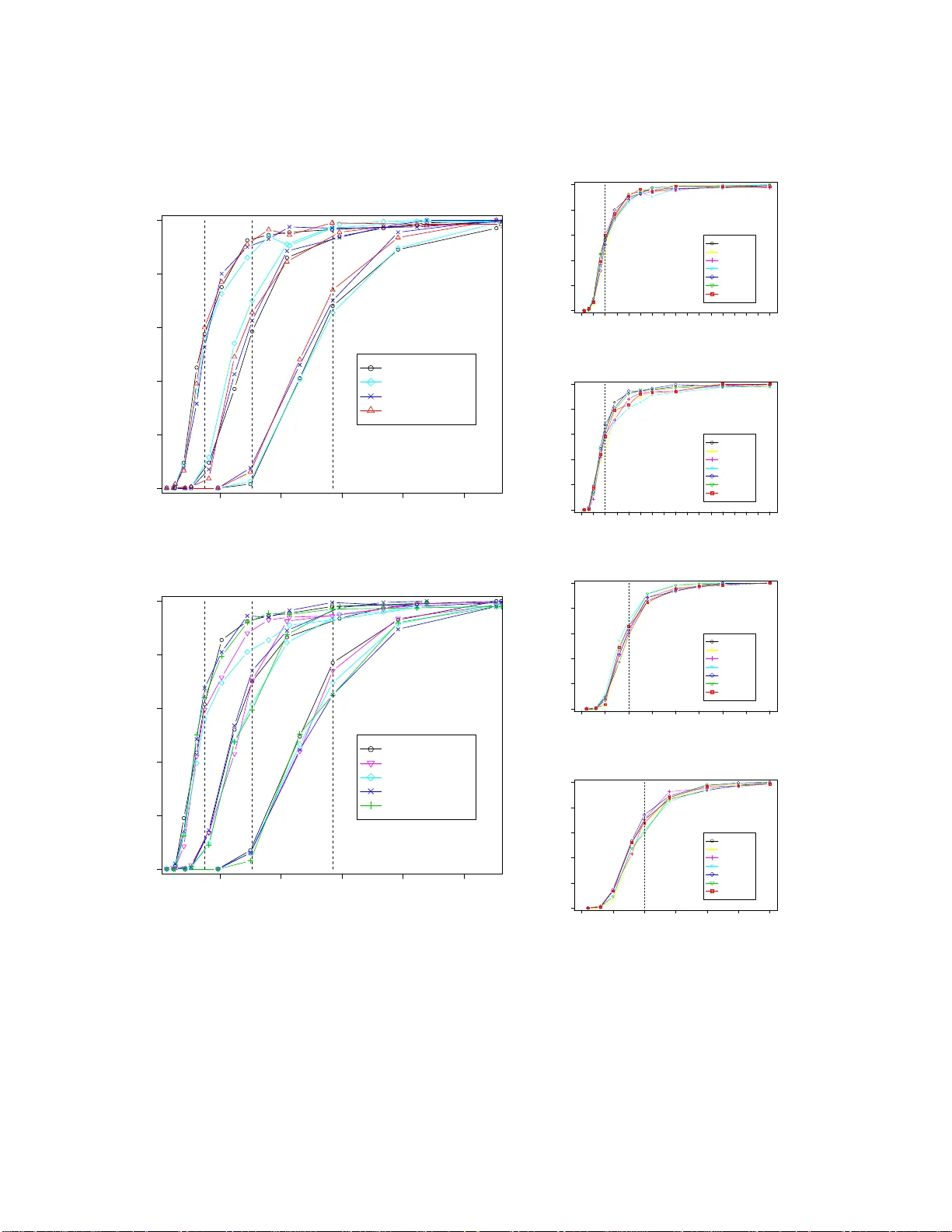
Compr essed Regr ession Shuheng Zhou ∗ John Laf ferty ∗ † Larry W asserman ‡ † ∗ Computer Science Department † Machine Learning Department ‡ Department of Statistics Carnegie Mellon Uni versity Pittsbur gh, P A 152 13 November 26, 2024 Abstract Recent research has studied the role of sparsity i n high dimens ional re gressi on and signal reconstruction, establishing theoretical limits for recovering sparse models from sparse data. This li ne of w ork shows that ℓ 1 -regularized least squares re gress ion can accurately estimate a sparse linear model from n noisy examples in p d imensions, e ven if p is much larger than n . In this paper we stu dy a variant of this problem where the original n input va riabl es are c om pressed by a random linear transformati on to m ≪ n examples in p dimensions, and establish conditi ons under which a sparse linear m odel can be successfull y rec overed from the compressed data. A primary mot i vation for this compression procedure is to anonymize th e data and preserve p ri vac y by reveal- ing little information about the original data. W e characterize the number of random projections that are required fo r ℓ 1 -regularized compressed regression to identify the nonzero coefﬁc i ents in the true model wi th prob ability approaching one, a property called “sparsistence. ” In addition, we show that ℓ 1 -regularized compressed re gression asymptoticall y predicts as well as an oracle linear model, a p roperty called “persis- tence. ” Finally , we characterize the priv acy properties of the compression procedure in inform ation-theoretic terms, e st ablishing upper boun ds on the mutual information between the compressed and uncompressed data that decay to zero. Keyw ords: Sparsity , ℓ 1 regularization, las so, high dimensional regression, priv acy , capacity of multi-antenna channels, compressed sensing. 1 C O N T E N T S 1 Intr oduction 3 2 Backgr ound an d Related W o rk 6 2.A Sparse Re gress ion . . . . . . . . . . . . . . . . . . . . . . . . . . . . . . . . . . . 6 2.B Compressed Sensing . . . . . . . . . . . . . . . . . . . . . . . . . . . . . . . . . 8 2.C Pri vacy . . . . . . . . . . . . . . . . . . . . . . . . . . . . . . . . . . . . . . . . 9 3 Compr essed Regr ession is Sparsistent 10 3.A Outline of Proof for Theorem 3.4 . . . . . . . . . . . . . . . . . . . . . . . . . . . 13 3.B Incoherence and Concentration Under Random Projection . . . . . . . . . . . . . 14 3.C Proof of Theorem 3.4 . . . . . . . . . . . . . . . . . . . . . . . . . . . . . . . . . 15 4 Compr essed Regression is P ersis tent 19 4.A Uncompressed Persistence . . . . . . . . . . . . . . . . . . . . . . . . . . . . . . 20 4.B Compressed Persistence . . . . . . . . . . . . . . . . . . . . . . . . . . . . . . . . 22 5 Inf ormatio n Theore tic Analysis of Privacy 26 5.A Pri vacy Und er the Multiple Antenna Channel Model . . . . . . . . . . . . . . . . 27 5.B Pri vacy Und er Multiplicativ e Noise . . . . . . . . . . . . . . . . . . . . . . . . . . 28 6 Experiments 30 6.A Sparsistency . . . . . . . . . . . . . . . . . . . . . . . . . . . . . . . . . . . . . . 30 6.B Persistence . . . . . . . . . . . . . . . . . . . . . . . . . . . . . . . . . . . . . . 37 7 Pr o o fs of T echnical Results 40 7.A Connection to the Gaussian Ensemble Result . . . . . . . . . . . . . . . . . . . . 40 7.B S -Incoherence . . . . . . . . . . . . . . . . . . . . . . . . . . . . . . . . . . . . . 42 7.C Proof of Lemma 3.5 . . . . . . . . . . . . . . . . . . . . . . . . . . . . . . . . . . 43 7.D Proof of Proposition 3.6 . . . . . . . . . . . . . . . . . . . . . . . . . . . . . . . . 46 7.E Proof of Theorem 3.7 . . . . . . . . . . . . . . . . . . . . . . . . . . . . . . . . . 49 7.F Proof of Lemma 3.8 . . . . . . . . . . . . . . . . . . . . . . . . . . . . . . . . . . 52 7.G Proof of Lemma 3.10 . . . . . . . . . . . . . . . . . . . . . . . . . . . . . . . . . 54 7.H Proof of Claim 3.11 . . . . . . . . . . . . . . . . . . . . . . . . . . . . . . . . . . 54 8 Discussion 55 9 Acknowledgmen ts 56 2 I . I N T RO D U C T I O N T wo issues facing the use of statis tical learning m ethods in applications are s cale and privacy . Scale is an issue i n storing, manipul ating and ana l yzing extremely large, high dimensional data. Pri vacy is, increasingly , a concern whene ver large amounts of conﬁdential data are manipulated within an o r ganization. It is often important to allo w researchers to analyze data without compro- mising the priv acy of customers or leaking c o nﬁdential informati on outside t he organization. In this paper we show that sparse regression for hi gh dimensional data can be carried out di rec t ly on a compressed form of the data, in a mann er that can be shown to guard p ri vac y i n an information theoretic sense. The app roach we de velop here compresses the data by a random l inear or af ﬁne transformation, reducing t he number of data records exponenti ally , while preserving t he number of orig inal input var i ables. These com pressed data can then be made av ail able for statisti cal analyses; we focus on the problem of sparse linear re gressio n for high d imensional data. I nform ally , our theory ens ures that the rele vant predictors c an be l ea rned from t he compressed data as well as they cou ld be f rom the original uncompressed da t a. Moreover , the actual predictions ba s ed on ne w examples a re as accurate as the y would be had the origi nal data been made av ailabl e. Howe ver , the original data are not recove rable from the compressed data, and the compressed data ef fectively r eveal no more information th an would be revea l ed by a com pletely ne w s ample. At the same time, t he inference algorithms run faster and require fe wer resources t han th e much lar ger uncom pressed data would require. In f act, the original data need never be s tored; they can be transformed “on the ﬂy” as they come in. In more detail, the d ata are re present ed as a n × p matrix X . Each of the p colum ns is an attrib ute, and ea ch of the n rows is the vector of attributes for an individual record. The data ar e com pressed by a random linear transformation X 7→ e X ≡ 8 X (1 . 1) where 8 is a random m × n matrix with m ≪ n . It is also natural to consider a random afﬁne transformation X 7→ e X ≡ 8 X + 1 (1 . 2) where 1 is a random m × p matrix. Such transformations have been called “matrix masking ” in the priv acy l iterature (Duncan and Pearson, 199 1 ). The entries of 8 and 1 are taken t o be in dependent Gaussian random variables, but other distributions are poss ible. W e think of e X as “public, ” while 8 and 1 are pri vate and only needed at the time of com pression. H o wev er , e ven with 1 = 0 and 8 known, recovering X from e X requires solving a highly under -determined linear system a nd comes with information theoretic priv acy guarantees, as we demonstrate. 3 In standard regression, a response Y = X β + ǫ ∈ R n is associated with the input variables, where ǫ i are ind ependent, mean zero addi ti ve noise variables. In compress ed re gression, we assume th at the response is also compressed, resulting in the transformed response e Y ∈ R m giv en by Y 7→ e Y ≡ 8 Y (1 . 3) = 8 X β + 8ǫ (1 . 4) = e X β + e ǫ (1 . 5) Note that under compression, the transformed noise e ǫ = 8ǫ is not independ ent across examples. In the sparse setting, the parameter v ector β ∈ R p is sparse, with a relatively sm all number s of nonzero coefﬁcients sup p (β ) =  j : β j 6= 0  . T wo key tasks are to identify the relev ant variables, and to predict the response x T β for a ne w input vector x ∈ R p . The m ethod we focus o n is ℓ 1 - regularized least squares, also known as the lasso (T i bshirani , 1996). The main contributions of this paper are tw o technical re su lts on the performance of this est imator , and an information- theoretic analysis of the pri vacy properties of the procedure. Our ﬁrst result shows t hat t he lasso is sparsistent u nder compressi on, m eaning that the correct s parse set of relev ant variables is identiﬁed asymptoticall y . Omitting details and technical assumptions for clarity , our result is the following. Sparsistence (Theor em 3.4): If the number of compressed examples m satisﬁes C 1 s 2 log n p s ≤ m ≤ s C 2 n log n , (1 . 6) and the regularization para m eter λ m satisﬁes λ m → 0 and m λ 2 m log p → ∞ , (1 . 7) then the compressed lasso solutio n e β m = arg min β 1 2 m k e Y − e X β k 2 2 + λ m k β k 1 (1 . 8) includes the correct va riabl es, asymptot ically: P  supp ( e β m ) = supp (β )  → 1 . (1 . 9) Our second re su lt shows that the lasso is persistent under compression. Roughly speaking, per- sistence (Greenshtein and Ritov, 2004) means that the procedure predicts well, as measured by the predictiv e risk R (β ) = E ( Y − X β ) 2 , (1 . 10) where no w X ∈ R p is a ne w input vector and Y is the ass ociated respon se. Persistence is a weaker condition than sparsistency , and in particular does not assume that the true model is lin ear . 4 Pe rsi stenc e (Theorem 4.1): Giv en a sequence of sets o f estimators B n , m , the sequence of com- pressed lasso estimators e β n , m = ar g m in k β k 1 ≤ L n , m k e Y − e X β k 2 2 (1 . 11) is persistent with the oracle risk ov er uncompressed data with respect to B n , m , meaning that R ( e β n , m ) − inf k β k 1 ≤ L n , m R (β ) P − → 0 , as n → ∞ . (1 . 12) in case log 2 ( n p ) ≤ m ≤ n and the radius of the ℓ 1 ball satisﬁes L n , m = o ( m / log ( n p ) ) 1 / 4 . Our third result analyzes the pri vac y properties of compressed regression. W e consi der t he prob- lem of recove ring the uncomp ressed data X from the compressed data e X = 8 X + 1 . T o pre- serve pri vacy , t he random matrices 8 and 1 shoul d remain pri vate. Howe ver , ev en in the case where 1 = 0 and 8 is known, if m ≪ min ( n , p ) the linear system e X = 8 X is highly under - determined. W e ev aluate priv acy in i nformation theoretic terms by b ounding the ave rage mutual information I ( e X ; X )/ n p per matrix entry in th e original data matrix X , wh ich can be viewed a s a communication rate. Bounding this m utual information is int imately connected with t he probl em of computi ng the channel capacity of certain mul tiple-antenna wireless communication systems (Marzetta and Hochwald, 1999; T elatar, 1999). Inf ormatio n Resistence (Pr oposi ti o ns 5.1 and 5.2): The ra t e at which information about X is re vealed by the compressed data e X satisﬁes r n , m = sup I ( X ; e X ) n p = O  m n  → 0 , (1 . 13) where the supremum is over distributions on the original data X . As summarized by these result s, compressed re gression is a practical procedure for sparse learning in high dimensional data that has prov ably good properties. This basic technique has connecti ons in the pri vacy literature with matrix m asking and other methods, yet most of the e xis ting work in this direction has been heuristic and without theoretical gu ara nt ees; connecti ons with this literature are brieﬂy revie wed i n Section 2.C. Compressed regression b ui lds on the ideas und erlying compressed sensing and sparse inference in high dim ensional data, topi cs which hav e attracted a great deal of recent interest in the stati stics and signal processing comm unities; the connections with this literature are re viewed in Section 2.B and 2.A. The remainder of the p aper is or ganized as follo ws. In Section 2 we revie w rele vant work from high dim ensional statisti cal inference, comp ressed sensing and priv acy . Section 3 presents ou r analysis of the sparsistency properties of the c o mpressed lasso. Our approach follo ws the m ethods introduced by W ainwright (2006) in t he uncompressed case. Section 4 proves that compress ed 5 regression is persi stent. Section 5 derives upper bounds on the mutual information between the compressed data e X and the uncompressed data X , after i dentifying a correspondence with the problem of compu ting channel capacity for a certain model of a mu ltiple-antenna mobile com- munication channel. Section 6 includ es the result s o f experimental simulat ions, showing that t he empirical performance of the compressed lasso is consist ent with our theoretical analysis. W e e valuate the abi lity of the procedure t o recover the relev ant v ariables (sp arsistenc y ) and to predict well (persistence). The technical details o f the proof of sparsistency are collected at the end o f the paper , in Se cti on 7 .B. The paper concludes wi th a discussi on of the resul ts and directions for future work in Section 8. I I . B A C K G R O U N D A N D R E L A T E D W O R K In this sectio n we brieﬂy revie w relev ant related work in high dimensional statist ical inference, compressed sensing, and priv acy , to place our work in conte xt . A. Sparse Re gression W e adopt stand ard notati on where a data matrix X has p var i ables and n records; in a l inear mod el the response Y = X β + ǫ ∈ R n is thus an n -v ector , and the noise ǫ i is independent and mean zero, E (ǫ ) = 0. The usual estimator of β is the least squares estimator b β = ( X T X ) − 1 X T Y . (2 . 1) Howe ver , t his estimator h as very lar g e variance when p is large, and i s not even deﬁned when p > n . An estimator that has recei ved m uch attent ion i n the recent literature is the lasso b β n (T ibshi rani , 1996), deﬁned as b β n = ar g mi n 1 2 n n X i = 1 ( Y i − X T i β ) 2 + λ n p X j = 1 | β j | (2 . 2) = ar g mi n 1 2 n k Y − X β k 2 2 + λ n k β k 1 , (2 . 3) where λ n is a regularization parameter . The prac t ical s uccess and importance o f th e l asso can b e attributed t o the fact that in many cases β is sparse, that is , it has fe w lar ge compon ents. For example, data are often collected with many v ariables in the hope that at least a few will be useful for prediction. The result is that many cov ariates contribute little to the prediction of Y , although it is not kno wn in adv ance which v ariables are important. Recent work h as greatly clariﬁed the properties of the lasso estimator in the high dimensional setting. One of the most basic desirable p roperties of an est imator is consisistency; an estimator b β n is 6 consistent in case k b β n − β k 2 P → 0 . (2 . 4) Meinshausen and Y u (2006) have recently shown that the l asso is consistent in the hig h dimen- sional setting. If the und erlying model is sparse, a natural yet m ore demandi ng criterion is t o ask that the estimator correctly identify th e rele vant variables. This may be useful for interpretation, dimension reduction and prediction. For example, if an ef fective procedure for high-dim ensional data c an be used to identify the rele vant variables in the m odel, then these variables can be isolated and their coefﬁ cient s estimated by a separate procedure that works well for low-dimensional data. An estimator is sparsistent 1 if P  supp ( b β n ) = supp (β )  → 1 , (2 . 5) where supp (β ) = { j : j 6= 0 } . Asymptotically , a sparsis tent esti mator has nonzero coef ﬁ- cients only for the true relev ant var i ables. Sparsistency proofs for high d imensional problems hav e appeared recently in a num ber o f s ettings. M einshausen and Buhlmann (2006) consider the problem of estimating the graph underlyin g a sparse Gaussi an g raphical m odel by sho wi ng spar- sistency of the lasso with exponential rates of con ver gence on the p robability of error . Zhao and Y u (2007) show sparsistency of the l asso und er more general noi se distributions. W ainwrig ht (2006) characterizes the sparsistency properti es of the lass o by showing t hat there is a threshold sample size n ( p , s ) abo ve which the rele vant v ariables are identiﬁed, and below which the rele vant v ari- ables f ail to be identiﬁed, where s = k β k 0 is the num ber of relev ant v ariables. More precisely , W ainwright (2006) sho ws that when X comes from a Gaussian ensemble, there exist ﬁxed con- stants 0 < θ ℓ ≤ 1 and 1 ≤ θ u < +∞ , where θ ℓ = θ u = 1 when e ach row of X is chosen as an independent Gaussian random vector ∼ N ( 0 , I p × p ) , then for any ν > 0, if n > 2 (θ u + ν ) s log ( p − s ) + s + 1 , (2 . 6) then the lasso identiﬁes the true var i ables with probability approaching one. Con versely , if n < 2 (θ ℓ − ν ) s log ( p − s ) + s + 1 , (2 . 7) then the probability of reco vering the true v ariables using the lasso approaches ze ro. These results require certain incoher ence ass umptions on the data X ; intui ti vely , it i s required that an irrele- vant variable cannot be too strongly correlated wi th the set of re l e vant v ariables. This result a nd W ainwright’ s m ethod of analys is are particularly relev ant to the current paper; the details will be described in t he following s ection. In particular , we refer to th is result as the Gaus sian Ensemb le result. Howe ver , it is im portant to point out that u nder compressi on, the noi se e ǫ = 8ǫ is not independent. T his prevents one from si mply applying the Gaussian Ens emble results to the com - pressed case. Related work that studi es inform ation theoretic li mits of sparsity re covery , where 1 This termino logy is due to Pradeep Ravikumar . 7 the particular estim ator i s not speciﬁed, includ es (W ainwrigh t , 2007; Donoho and T anner, 2006 ). Sparsistency in t he classiﬁcation s etting, with e xpon ential rates of con ver gence for ℓ 1 -regularized logistic regression, is studied by W ainwright et al. (2007). An alternativ e goal is accurate prediction. In high dim ensions it is essential to regularize the model in some fashion in order to con trol the var i ance of the est imator and attain go od predictive risk. Persistence for the lasso was ﬁrst deﬁned and studi ed by Greenshtein and Ritov (2004). Given a sequence of sets of estimators B n , the sequence of estimators b β n ∈ B n is called persistent in case R ( b β n ) − i nf β ∈ B n R (β ) P → 0 , (2 . 8) where R (β ) = E ( Y − X T β ) 2 is the predictio n risk o f a ne w pair ( X , Y ) . Thus, a sequence of estimators is persi stent if it asymptotically predicts as well as the oracle within t he class, which minimizes t he population risk; it can be achieved under weaker assum ptions than are required for sparsistence. In particular , persistence does not a s sume t he true model is linear , and it does not require strong incoherence assumpt ions on the data. The results of th e current paper show that sparsistence and persistence are preserved under compression. B. Compr essed Sensing Compressed regression has clo se connections to, and dra ws motiv ation from, compressed sens ing (Donoho, 2006; Cand ` es et al., 2006; Cand ` e s and T a o, 2 006; R auhut et al., 200 7 ). Howe ver , in a sense, our motiva t ion here is the opposite t o that of compressed sensing. While compressed sens ing of X allows a sparse X to b e reconst ructed from a small n umber of random measurements, our goal is to reconstruct a sparse functio n of X . Indeed, from th e point of vie w of priv acy , approximately reconstructing X , which compressed sensing sho ws is possible if X is sparse, should be vie wed as undesirable; we return to this point in Section 5. Se veral authors have c o nsidered v ariations on comp ressed sensing for statistical signal processing tasks (Duarte et al., 2006; Davenport et al., 200 6 ; Haupt et al., 2 006; Dav enport et al., 2 007) . The focus of this w ork i s to consider certain hypoth esis testing problems under sparse random mea- surements, and a generalization to classiﬁcation of a signal in to t w o or mo re class es. Here one observes y = 8 x , where y ∈ R m , x ∈ R n and 8 i s a known random measurement matrix. The problem is to select between the hypotheses e H i : y = 8 ( s i + ǫ ), (2 . 9) where ǫ ∈ R n is additi ve Gaussian n oise. Importantly , the setup exploits t he “univer s ality” of the matrix 8 , which is not selected with knowledge of s i . The p roof techniques use con centration prop- erties of random projectio n, which underlie the celebrated lemma of Johnso n and Lindenstrauss (1984). The compressed regression problem we int roduce can be considered as a more challeng- ing statist ical i nfere nce task, where the problem is to select from an exponentially large s et of linear 8 models, each with a certain set of relev ant v ariables with unknown parameters, or to predict as well as the best linear model in s ome class. M oreo ver , a ke y mot i vation for compressed regression is priv acy; if pri vacy is not a concern, simple subs ampling of the data matrix could be an ef fectiv e compression procedure. C. Privacy Research on privac y in st atistical data analysis has a lon g hi story , going b ac k at least to Dalenius (1977a); we refer to Duncan and Pearson (1991) for discussion and further pointers into this lit- erature. The compression method we employ ha s been called matrix maskin g in the pri vac y lit- erature. In the general method , the n × p data matrix X is transform ed by pre-multiplication, post-multi plication, and additi on i nto a ne w m × q matrix e X = A X B + C . (2 . 10) The transformation A operates on data records for ﬁxed covariates, and the transformation B op- erates on cov ariates for a ﬁxed record. The method encapsulated in this transformation is quit e general, a nd allows the possibili ty of deleting records, suppressing subsets of variables, data swa p- ping, and includin g simulated data. In our use of matrix masking, we tra ns form t he data by re- placing each v ariable w ith a relatively small number of r ando m a verages of the instances of that var i able in the data. In other work, Sanil et al. (2004) consider t he problem of p ri vac y preserving regression analysis i n di strib uted data, where different variables appear i n dif ferent databases but it is of interest to int e grate data across databases. The recent work of Ting et al. (2007) con siders random orthogonal mappin gs X 7→ R X = e X where R is a random rotation (rank n ), designed to preserve th e sufﬁcient s tatistics of a multiv ariate Gaussi an and therefore allo w regression est ima- tion, for instance. This use of matrix masking d oes not share t he information theoretic guarantees we present in Section 5. W e are not a ware of pre vio us work that analyzes the asymptotic prop erties of a statistical estimator under matrix masking in the high dimensional setting. The w ork of Liu et al. (2006) is closely related to t he current paper at a high le vel, in that it consid- ers low rank random linear transformations of either the ro w space or column space of the data X . Liu et al. (2006) note the J ohnson-Lindenstrauss lemma, w hich implies that ℓ 2 norms are approx- imately preserved under random p rojection, and ar gue heuris tically that data m ining procedures that e xploi t correlations or pairwise distances in th e data, such as principal compon ents analysis and clu stering, are just as effe ctive under random projection . The priv acy analysis i s restricted to observing that recovering X from e X requires solving an under-determined linear s ystem, and ar gui ng that this pre vents the e xact values fr o m being reco vered. An i nformation-theoretic quantiﬁcation of priv acy was formulated by Agrawal and Aggarw al (2001). Giv en a r ando m variable X and a transformed va riabl e e X , Agrawa l and Aggarwal (2001) deﬁne 9 the conditional priv acy loss of X given e X as P ( X | e X ) = 1 − 2 − I ( X ; e X ) , (2 . 11) which is s imply a transformed measure of the mutual i nformation between the two random vari- ables. In our work we id entify priv acy w ith the rate of information com municated about X through e X under matrix maski ng, maximizing ove r all di strib uti ons on X . W e furthermore identify thi s with the problem of compu ting, or boundi ng, the Shannon capacity of a multi-antenna wireless communication channel, as modeled by T elatar (1999) and Marzetta and Hochwald (1999). Finally , i t is important to mention the extensiv e and curre nt ly a ctive line of w ork o n cryptographic approaches t o priv acy , w hich have come mainly from the theoretical computer science community . For instance, Feigenbaum et al. (2006) d e velop a framew o rk for secure comput ation of approx- imations; intuit i vely , a priv ate approx imation of a fun ction f is an approxim ation b f that does not re veal information about x other than what can be deduced from f ( x ) . Indyk and W oodruff (2006) consider the problem of computing pri vate approximate nearest neighbors i n this setting. Dwork (2006) r evisits the notion of pri vac y formulated by Dalenius (1977b), which intuitiv ely de- mands that n othing can be learned about an indi vi dual r ecord in a d atabase that cannot b e learned without ac cess to the database. An impossibili ty resul t is gi ven whi ch shows that, appropriately formalized, this s trong notion of privac y cannot be achie ved. An alternati ve n otion of differ ential privacy is proposed, which allows the prob ability of a disclosure of priv ate inform ation to change by only a small multiplicative fac t or , depending on whether or not an indi vidual par t icipates in th e database. This line of work has recently been b ui lt upon by Dw ork et al . (2007), with connections to compressed sensi ng, showing that any method that giv es accurate answers to a large fraction of randomly generated subset sum queries must violate priv acy . I I I . C O M P R E S S E D R E G R E S S I O N I S S PA R S I S T E N T In the standard setting, X is a n × p m atrix, Y = X β + ǫ is a vector of noisy observations und er a linear m odel, and p is cons idered to b e a constant. In the high-dimensional setting we all o w p to grow with n . The lasso re fers t o the following quadratic program: ( P 1 ) minim ize k Y − X β k 2 2 such that k β k 1 ≤ L . (3 . 1) In Lagrangian form, this becomes the optimizatio n probl em ( P 2 ) minimize 1 2 n k Y − X β k 2 2 + λ n k β k 1 , (3 . 2) where the s caling factor 1 / 2 n is chosen by conv entio n and con venience . F or an appropriate cho ice of the regularization para m eter λ = λ( Y , L ) , the solut ions of these two problems coincide. 10 In compressed regression we project each column X j ∈ R n of X to a s ubspace of m dimensions, using an m × n random projection matri x 8 . W e shall assum e t hat the entries of 8 are independent Gaussian random v ariables: 8 i j ∼ N ( 0 , 1 / n ). (3 . 3) Let e X = 8 X be th e com pressed m atrix of covariates, and let e Y = 8 Y be the compressed response. Our obj ecti ve is t o estimate β in order to determi ne the relev ant var i ables, or t o predict well. The compressed lasso is the optimization problem, for e Y = 8 X β + 8ǫ = 8 e X + e ǫ : ( e P 2 ) minimize 1 2 m k e Y − e X β k 2 2 + λ m k β k 1 , (3 . 4) with e  m being the set of optimal solution s: e  m = arg m in β ∈ R p 1 2 m k e Y − e X β k 2 2 + λ m k β k 1 . (3 . 5) Thus, the transformed noise e ǫ is no longer i .i.d., a fact that com plicates the analysis. It is conv enient to formalize the model selection problem using the following deﬁnitions. Deﬁnition 3.1. (Sign Consistency) A set of estimators  n is sign consistent with the true β if P  ∃ b β n ∈  n s.t. sgn ( b β n ) = sgn (β )  → 1 as n → ∞ , (3 . 6) where sgn ( · ) is giv en by sgn ( x ) =        1 if x > 0 0 if x = 0 − 1 if x < 0 . (3 . 7) As a shorthand, we use E  sgn ( b β n ) = sgn (β ∗ )  : =  ∃ b β ∈  n such that sgn ( b β ) = sgn (β ∗ )  (3 . 8) to denote the ev ent that a sign consistent solution exists. The l asso objective function is c onv ex in β , and strictl y con ve x for p ≤ n . Therefore the set of solutions to the lasso and comp ressed lasso (3 . 4) is con ve x: if b β and b β ′ are two solut ions, then by con vexity b β + ρ ( b β ′ − b β ) is also a solution for any ρ ∈ [0 , 1]. Deﬁnition 3.2. (Sparsistency) A set of estimators  n is sparsistent with the true β if P  ∃ b β n ∈  n s.t. supp ( b β n ) = supp (β )  → 1 as n → ∞ , (3 . 9) 11 Clearly , if a set o f estim ators is sign consistent then it is sparsistent. Although sparsistency is the primary goal in selecting the correct var i ables, ou r analysi s establishes conditions for the slightly stronger property of sign consistency . All recent work establis hing results o n sparsity recovery ass umes some form of incoher ence condi- tion on the data matrix X . Such a conditi on ensures t hat the irrelev ant variables are not to o stron gly correlated with t he relev ant va riabl es. Intuitively , wi thout s uch a condition the lasso m ay be sub- ject to false pos iti ves and negatives, where an rele vant variable i s replaced by a highly correlated rele vant variable. T o formulate such a condition, it is con v enient to introduce an a d ditional piece of notation. Let S = { j : β j 6= 0 } be the set of relev ant v ariables and let S c = { 1 , . . . , p } \ S be the set of irrele vant variables. Then X S and X S c denote the correspondi ng sets of columns of the matrix X . W e will impose the following incoherence condition; related conditions are used by Donoho et al. (2006) and T ropp (2004) in a determinis tic set ting. Deﬁnition 3.3. ( S -Incoher ence) Let X be an n × p matrix and let S ⊂ { 1 , . . . , p } be n onempty . W e say that X is S -incoher ent in case   1 n X T S c X S   ∞ +   1 n X T S X S − I | S |   ∞ ≤ 1 − η , for some η ∈ ( 0 , 1] , (3 . 10) where k A k ∞ = max i P p j = 1 | A i j | denotes the matrix ∞ -norm. Although it is not explicitly required, we only apply t his deﬁnition to X such that colum ns of X satisfy   X j   2 2 = 2 ( n ), ∀ j ∈ { 1 , . . . , p } . W e can now state the main result of this section. Theor em 3.4. Suppose that, before compressi on, we have Y = X β ∗ + ǫ , w here each colum n of X is normalized to ha ve ℓ 2 -norm n , and ε ∼ N ( 0 , σ 2 I n ) . Assume that X is S -incoherent, where S = supp (β ∗ ) , and deﬁne s = | S | and ρ m = min i ∈ S | β ∗ i | . W e observe, after compression, e Y = e X β ∗ + e ǫ , (3 . 11) where e Y = 8 Y , e X = 8 X , and e ǫ = 8ǫ , where 8 i j ∼ N ( 0 , 1 / n ) . Suppose  16 C 1 s 2 η 2 + 4 C 2 s η  ( ln p + 2 l og n + log 2 ( s + 1 )) ≤ m ≤ r n 16 log n (3 . 12) with C 1 = 4 e √ 6 π ≈ 2 . 504 4 and C 2 = √ 8 e ≈ 7 . 6885 , and λ m → 0 satisﬁes ( a ) m η 2 λ 2 m log ( p − s ) → ∞ , and ( b ) 1 ρ m ( r log s m + λ m    ( 1 n X T S X S ) − 1    ∞ ) → 0 . (3 . 13) Then the compressed lasso is sparsistent: P  supp ( e β m ) = supp (β )  → 1 as m → ∞ , (3 . 14) where e β m is an optimal solution to (3 . 4) . 12 A. Outline of Pr oof for Theor em 3.4 Our overall approach is to follow a deterministic analysis, in the sense that we analyze 8 X as a realization from the distribution of 8 from a Gaussian ensemble. Assuming that X sati sﬁes the S -incoherence condition, we show that with hi gh probabili ty 8 X also satisﬁes t he S -incoh ere nce condition, and hence th e incoherence conditi ons (7 . 1a) and (7 . 1b) used by W ainwrigh t (2006). In addition, we make use of a lar ge deviation result that sho ws 88 T is concentrated around its mean I m × m , which is crucial for the recov ery o f the true sparsity pattern. It is important to n ote that the compressed noise e ǫ is not independent and identically distributed, even when conditioned on 8 . In more detail, we ﬁ rst show that with high probability 1 − n − c for some c ≥ 2, the projected data 8 X satis ﬁes the following properties: 1. Each column of e X = 8 X has ℓ 2 -norm at most m ( 1 + η / 4 s ) ; 2. e X is S -incoherent, and also satisﬁes the incoherence conditions (7 . 1a) and (7 . 1b). In addition, the projections satisfy the following properties: 1. Each entry of 88 T − I is at most p b log n / n for some constant b , with high probability; 2. P  | n m h 8 x , 8 y i − h x , y i| ≥ τ  ≤ 2 exp  − m τ 2 C 1 + C 2 τ  for an y x , y ∈ R n with k x k 2 , k y k 2 ≤ 1. These facts allow us to condition on a “go od” 8 and incoherent 8 X , and to proceed as i n the deterministic setting wi th Gaussian noise. Our analysis then foll o ws that of W ainwright (2006). Recall S is the set of relev ant variables in β and S c = { 1 , . . . , p } \ S is the set of irrelev ant var i ables. T o explain the basic approach, ﬁrst ob serv e that t he KKT conditions imply that e β ∈ R p is an optimal solution to (3 . 4), i.e., e β ∈ e  m , if and only if there exists a subgradient e z ∈ ∂ k e β k 1 =  z ∈ R p | z i = s gn ( e β i ) for e β i 6= 0, and   e z j   ≤ 1 otherwise  (3 . 15) such that 1 m e X T e X e β − 1 m e X T e Y + λ e z = 0 . (3 . 16) Hence, the E  sgn ( e β ) = sgn (β ∗ )  can be shown t o be equiv alent to requiring t he existence of a solution e β ∈ R p such that s gn ( e β ) = sgn (β ∗ ) , and a subgradient e z ∈ ∂ k e β k 1 , such that the fol lo wing equations hold: 1 m e X T S c e X S ( e β S − β ∗ S ) − 1 m e X T S c e ǫ = − λ e z S c , (3 . 17a) 1 m e X T S e X S ( e β S − β ∗ S ) − 1 m e X T S e ǫ = − λ e z S = − λ sgn (β ∗ S ), (3 . 17b) 13 where e z S = s gn (β ∗ S ) and | e z S c | ≤ 1 by deﬁniti on of e z . The existence of sol utions to equations (3 . 17a) and (3 . 17b) can be characterized in terms of two e vents E ( V ) and E ( U ) . The proof pro- ceeds by showing that P ( E ( V )) → 1 and P ( E ( U )) → 1 as m → ∞ . In the remainder of this section we present the main steps of the proo f, relegating th e technical details to Section 7.B. T o a void unnecessary clut ter i n notation, we wi ll use Z to denote the compressed data e X = 8 X and W to denot e the compressed response e Y = 8 Y , and ω = e ǫ t o denote the compressed noise. B. Incoher ence and Concentration Und er Random Pr oject ion In order for the estim ated e β m to be close to the solut ion of the uncompressed lasso, we require the stability of inn er products of columns of X under multipli cation wi th the random matrix 8 , in the sense that h 8 X i , 8 X j i ≈ h X i , X j i . (3 . 18) T ow ard this e nd we ha ve the following result, adapted from Rauhut et al . (20 07), where for each entry in 8 , the variance i s 1 m instead of 1 n . Lemma 3 .5 . (Adapted fr om Rauhut et al. (2007)) Let x , y ∈ R n with k x k 2 , k y k 2 ≤ 1 . Assu me that 8 is an m × n random matrix wi th independent N ( 0 , n − 1 ) entries (independent of x , y ). Then for all τ > 0 P     n m h 8 x , 8 y i − h x , y i    ≥ τ  ≤ 2 exp  − m τ 2 C 1 + C 2 τ  (3 . 19) with C 1 = 4 e √ 6 π ≈ 2 . 504 4 and C 2 = √ 8 e ≈ 7 . 6885 . W e ne xt summarize the properties o f 8 X that we requi re. The following result im plies that, with high probability , incohere n ce is preserved under random projection. Pr o posi tion 3.6. Let X be a (deterministic) design matrix that is S -incoherent wit h ℓ 2 -norm n , and let 8 be a m × n random matrix with independent N ( 0 , n − 1 ) entries. Suppose that m ≥  16 C 1 s 2 η 2 + 4 C 2 s η  ( ln p + c ln n + ln 2 ( s + 1 )) (3 . 20) for s ome c ≥ 2 , w here C 1 , C 2 are deﬁned in Lem ma 3.5. Then with probabil ity at least 1 − 1 / n c the following properties hold for Z = 8 X : 14 1. Z is S -incoherent; in particular:     1 m Z T S Z S − I s   ∞ −   1 n X T S X S − I s   ∞   ≤ η 4 , (3 . 21a)   1 m Z T S c Z S   ∞ +   1 m Z T S Z S − I s   ∞ ≤ 1 − η 2 . (3 . 21b) 2. Z = 8 X is incoherent in the sense of (7 . 1a) and (7 . 1b) :    Z T S c Z S  Z T S Z S  − 1    ∞ ≤ 1 − η / 2 , (3 . 22a) 3 min  1 m Z T S Z S  ≥ 3 η 4 . (3 . 22b) 3. The ℓ 2 norm of each column is approximately preserved, for all j :      8 X j   2 2 − m    ≤ m η 4 s . (3 . 23) Finally , we ha ve the fol lo wing lar ge de v iation result for the projectio n m atrix 8 , which guarantees that R = 88 T − I m × m is small entrywise. Theor em 3.7. If 8 is m × n random matrix with independent entries 8 i j ∼ N ( 0 , 1 n ) , th en R = 88 T − I satisﬁes P  max i | R i i | ≥ p 16 log n / n  ∪  max i 6= j | R i j | ≥ p 2 log n / n  ≤ m 2 n 3 . (3 . 24) C. Pr oof of Theor em 3.4 W e ﬁrst state necessary and su f ﬁcient conditions on the e vent E ( sgn ( e β m ) = sgn (β ∗ )) . Note th at this is essentially equiv alent to Lem ma 1 in W ainwri ght (2006); a proof of t his lemma is i ncluded in Section 7.F for completeness. Lemma 3 .8 . Assume that the matrix Z T S Z S is in vertible. Then for any giv en λ m > 0 and noise vector ω ∈ R m , E  sgn ( e β m ) = sgn (β ∗ )  holds if and only if the following t w o con ditions hold:    Z T S c Z S ( Z T S Z S ) − 1  1 m Z T S ω − λ m sgn (β ∗ S )  − 1 m Z T S c ω    ≤ λ m , (3 . 25a) sgn  β ∗ S + ( 1 m Z T S Z S ) − 1  1 m Z T S ω − λ m sgn (β ∗ S )   = sgn (β ∗ S ). (3 . 25b) 15 Let E b : = sgn (β ∗ S ) and e i ∈ R s be the ve ctor with 1 in i t h position, and zeros elsewhere; hence k e i k 2 = 1. Our p roof of Theorem 3.4 fol lo ws t hat of W ainwright (2006). W e ﬁrst deﬁne a set of random va riabl es that are rele vant to (3 . 25a) and (3 . 25b): ∀ j ∈ S c , V j : = Z T j n Z S ( Z T S Z S ) − 1 λ m E b + h I m × m − Z S ( Z T S Z S ) − 1 Z T S i ω m o , (3 . 26a) ∀ i ∈ S , U i : = e T i +  1 m Z T S Z S  − 1 h 1 m Z T S ω − λ m E b i . (3 . 26b) W e ﬁrst d eﬁ ne a set of random v ariables that are relev ant t o Condition (3 . 25a), which holds if and if only the e vent E ( V ) : =  max j ∈ S c   V j   ≤ λ m  (3 . 27) holds. F or Condition (3 . 25b), the e vent E ( U ) : =  max i ∈ S | U i | ≤ ρ m  , (3 . 28) where ρ m : = min i ∈ S | β ∗ i | , is sufﬁcient to guarantee that Condition (3 . 25b) holds. Now , in the proof of T heorem 3.4, we assum e that 8 h as been ﬁxed, and Z = 8 X and 88 T beha ve nicely , in accordance with the results of Section 3.B. Let R = 88 T − I m × m as d eﬁ ned in Theorem 3.7 . From here on, we use (   r i , j   ) to denote a ﬁxed s ymmetric matrix with diagonal entries that are p 16 log n / n and o f f-diagonal entries that are p 2 log n / n . W e now p ro ve that P ( E ( V ) ) and P ( E ( U ) ) both conv erge to one. W e begin by stating two technical lemmas that will be required. Lemma 3 .9 . (Gaussian Comparison) For any Gaussian random vector ( X 1 , . . . , X n ) , E  max 1 ≤ i ≤ n | X i |  ≤ 3 p log n max 1 ≤ i ≤ n q E  X 2 i  . (3 . 29) Lemma 3 .10. Suppose that   1 n X T S X S − I s   ∞ is bounded away from 1 and m ≥  16 C 1 s 2 η 2 + 4 C 2 s η  ( log p + 2 l og n + log 2 ( s + 1 )). (3 . 30) Then 1 ρ m ( r log s m + λ m     ( 1 n X T S X S ) − 1     ∞ ) → 0 (3 . 31) implies that 1 ρ m ( r log s m + λ m    ( 1 m Z T S Z S ) − 1    ∞ ) → 0 . (3 . 32) 16 Analysis of E ( V ) . Note that for each V j , for j ∈ S c , µ j = E  V j  = λ m Z T j Z S ( Z T S Z S ) − 1 E b . (3 . 33) By Proposition 3.6, we hav e that µ j ≤ λ m    Z T S c Z S  Z T S Z S  − 1    ∞ ≤ ( 1 − η / 2 )λ m , ∀ j ∈ S c , (3 . 34) Let us deﬁne e V j = Z T j nh I m × m − Z S ( Z T S Z S ) − 1 Z T S i ω m o , (3 . 35) from which we obtain max j ∈ S c   V j   ≤ λ m    Z T S c Z S  Z T S Z S  − 1    ∞ + max j ∈ S c   e V j   ≤ λ m ( 1 − η / 2 ) + max j ∈ S c   e V j   . (3 . 36a) Hence we need to show t hat P  max j ∈ S c | e V j | λ m ≥ η/ 2  → 0 . (3 . 37) It is sufﬁ cient to sh o w P  max j ∈ S c   e V j   ≥ η/ 2  → 0 . By Markov’ s inequality and the Gaussian comparison lemma 3.9, we obtain that P  max j ∈ S c e V j ≥ η/ 2  ≤ E  max j ∈ S c e V j  λ m (η/ 2 ) ≤ 6 p log ( p − s ) λ m η max j ∈ S c r E  e V 2 j  . (3 . 38) Finally , let us use P = Z S ( Z T S Z S ) − 1 Z T S = P 2 to represent the projection matrix. V ar ( e V j ) = E  e V j 2  (3 . 39a) = σ 2 m 2 Z T j n  ( I m × m − P ) 8   ( I m × m − P ) 8  T o Z j (3 . 39b) = σ 2 m 2 Z T j  I m × m − P  Z j + σ 2 m 2 Z T j ( R − P R − R P + P R P ) Z j (3 . 39c) ≤ σ 2 m 2   Z j   2 2 + σ 2 m 2 k R − P R − R P + P R P k 2   Z j   2 2 (3 . 39d) ≤ 1 + 4 ( m + 2 ) r 2 log n n ! σ 2 ( 1 + η 4 s ) m , ( 3 . 39e) where   Z j   2 2 ≤ m + m η 4 s by Proposition 3.6, and k R − P R − R P + P R P k 2 ≤ k R k 2 + k P k 2 k R k 2 + k R k 2 k P k 2 + k P k 2 k R k 2 k P k 2 (3 . 40a) ≤ 4 k R k 2 ≤ 4   (   r i , j   )   2 ≤ 4 ( m + 2 ) r 2 log n n , (3 . 40b) 17 giv en that k I − P k 2 ≤ 1 a n d k P k 2 ≤ 1 and the f act t hat ( | r i , j | ) i s a symmetric matrix, k R k 2 ≤   (   r i , j   )   2 ≤ q   ( | r i , j | )   ∞   ( | r i , j | )   1 =   ( | r i , j | )   ∞ (3 . 41a) ≤ ( m − 1 ) r 2 log n n + r 16 log n n ≤ ( m + 2 ) r 2 log n n . (3 . 41b) Consequently Condition (3 . 13 a ) is suf ﬁcient to ensure that E ( m a x j ∈ S c | e V j | ) λ m → 0 . Thus P ( E ( V ) ) → 1 as m → ∞ so long as m ≤ q n 2 log n . Analysis of E ( U ) . W e now show that P ( E ( U ) ) → 1 . Using the triangle inequality , we obtain the upper bound max i ∈ S | U i | ≤     1 m Z T S Z S  − 1 1 m Z T S ω    ∞ +     1 m Z T S Z S  − 1    ∞ λ m . (3 . 42) The second ℓ ∞ -norm is a ﬁx ed value given a deterministic 8 X . Hence we focus on the ﬁrst norm. W e now deﬁne, for all i ∈ S , th e Gaussian ra nd om v ariable G i = e T i  1 m Z T S Z S  − 1 1 m Z T S ω = e T i  1 m Z T S Z S  − 1 1 m Z T S 8ǫ . (3 . 43) Giv en that ǫ ∼ N ( 0 , σ 2 I n × n ) , we ha ve for all i ∈ S that E ( G i ) = 0 , (3 . 44a) V ar ( G i ) = E  G 2 i  (3 . 44b) = ( e T i  1 m Z T S Z S  − 1 1 m Z T S 8 ) n e T i  1 m Z T S Z S  − 1 1 m Z T S 8 o T V ar (ǫ i ) (3 . 44c) = σ 2 m e T i n  1 m Z T S Z S  − 1 1 m Z T S 88 T Z S  1 m Z T S Z S  − 1 o e i (3 . 44d) = σ 2 m e T i n  1 m Z T S Z S  − 1 1 m Z T S ( I + R ) Z S  1 m Z T S Z S  − 1 o e i (3 . 44e) = σ 2 m e T i  1 m Z T S Z S  − 1 e i + σ 2 m e T i n  1 m Z T S Z S  − 1 1 m Z T S R Z S  1 m Z T S Z S  − 1 o e i . (3 . 44f) W e ﬁrst bound the ﬁrst term of (3 . 44f). By (3 . 22b), we have that for all i ∈ S , σ 2 m e T i  1 m Z T S Z S  − 1 e i ≤ σ 2 m     1 m Z T S Z S  − 1    2 = σ 2 m 3 min  1 m Z T S Z S  ≤ 4 σ 2 3 m η . (3 . 45) W e next b ound the sec on d term of (3 . 44f). Let M = C B C m , wh ere C =  1 m Z T S Z S  − 1 and B = Z T S R Z S . By deﬁnit ion, e i = [ e i , 1 , . . . , e i , s ] = [0 , . . . , 1 , 0 , . . . ] , where e i , i = 1 , e i , j = 0 , ∀ j 6= i . (3 . 46) 18 Thus, for all i ∈ S , e T i n  1 m Z T S Z S  − 1 1 m Z T S R Z S  1 m Z T S Z S  − 1 o e i = s X j = 1 s X k = 1 e i , j e i , k M j , k = M i , i . (3 . 47) W e next require the follo win g fact. Claim 3.11. If m satisﬁes ( 3 . 12 ), then for all i ∈ S , we hav e max i M i , i ≤ ( 1 + η 4 s )  4 3 η  2 . The proof appears in Section 7.H. Usi ng Claim 3.11, we hav e by (3 . 45), (3 . 47) that max 1 ≤ i ≤ s q E  G 2 i  ≤ s  4 σ 3 η  2 1 m  3 η 4 + 1 + η 4 s  ≤ 4 σ 3 η s 1 m  1 + 3 4 + 1 4 s  . (3 . 48a) By the Gaussian comparison lemma 3.9, we ha ve E  max 1 ≤ i ≤ s | G i |  = E      1 m Z T S Z S  − 1 1 m Z T S ω    ∞  (3 . 49a) ≤ 3 p log s max 1 ≤ i ≤ s q E  G 2 i  ≤ 4 σ η r 2 log s m . (3 . 49b) W e no w app ly Markov’ s inequality t o show that P ( E ( U ) ) → 1 due to C ond ition (3 . 13 b ) in the Theorem statement and Lemma 3.10, 1 − P  sgn  β ∗ S + ( 1 m Z T S Z S ) − 1  1 m Z T S ω − λ m sgn (β ∗ S )   = s gn (β ∗ S )  ≤ P  max i ∈ S | U i | ≥ ρ m  (3 . 50a) ≤ P  max i ∈ S | G i | + λ m     1 m Z T S Z S  − 1    ∞ ≥ ρ m  (3 . 50b) ≤ 1 ρ m  E  max i ∈ S | G i |  + λ m     1 m Z T S Z S  − 1    ∞  (3 . 50c) ≤ 1 ρ m 4 σ η r 2 log s m + λ m     1 m Z T S Z S  − 1    ∞ ! (3 . 50d) → 0 . (3 . 50e) which completes the proof.  I V . C O M P R E S S E D R E G R E S S I O N I S P E R S I S T E N T 19 Persistence ( Greensht ein and Ritov (2004)) is a weaker condit ion than sparsistency . In particular , we drop the assumpti on that E ( Y | X ) = β T X . Roughly speaking, persistence implies that a pro- cedure predicts well. Let us ﬁrst re view the Greenshtein-Ritov argument; we then adapt it to t he compressed case. A. Uncompr essed P ersistence Consider a ne w pair ( X , Y ) and suppose we want t o predict Y from X . T he predictive risk using predictor β T X i s R (β ) = E ( Y − β T X ) 2 . (4 . 1) Note that t his is a wel l-deﬁned quantity e ven though we d o not assume that E ( Y | X ) = β T X . It is con venient to write the risk in the follo win g way . Deﬁne Q = ( Y , X 1 , . . . , X p ) and denote γ as γ = ( − 1 , β 1 , . . . , β p ) T = (β 0 , β 1 , . . . , β p ) T . (4 . 2) Then we can re writ e the risk as R (β ) = γ T 6 γ , (4 . 3) where 6 = E ( Q Q T ) . Th e training err o r is then b R n (β ) = 1 n P n i = 1 ( Y i − X T i β ) 2 = γ T b 6 n γ , wh ere b 6 n = 1 n Q T Q (4 . 4) and Q = ( Q † 1 Q † 2 · · · Q † n ) T where Q † i = ( Y i , X 1 i , . . . , X pi ) T ∼ Q , ∀ i = 1 , . . . , n , are i.i.d. random vectors. Let B n = { β : k β k 1 ≤ L n } , for L n = o  ( n / log n ) 1 / 4  . (4 . 5) Let β ∗ minimize R (β ) subject to β ∈ B n : β ∗ = arg min k β k 1 ≤ L n R (β ). (4 . 6) Consider the uncompressed lasso estimator b β n which minimizes b R n (β ) subject to β ∈ B n : b β n = arg m in k β k 1 ≤ L n b R n (β ). (4 . 7) Assumption 1. Let Q j , Q k denote elements of Q . Suppose that, for each j and k , E  | Z | q  ≤ q ! M q − 2 s / 2 , (4 . 8) for every q ≥ 2 and some con stants M and s , where Z = Q j Q k − E ( Q j Q k ) . Then, by Bernstein’ s inequality , P     b 6 n j k − 6 j k    > ǫ  ≤ e − cn ǫ 2 (4 . 9) 20 for some c > 0. Hence, if p n ≤ e n ξ for some 0 ≤ ξ < 1 then P  max j , k    b 6 n j k − 6 j k    > ǫ  ≤ p 2 n e − cn ǫ 2 ≤ e − cn ǫ 2 / 2 . (4 . 10) Hence, if ǫ n = q 2 log n cn , then P  max j , k    b 6 n j k − 6 j k    > ǫ n  ≤ 1 n → 0 . (4 . 11) Thus, max j , k | b 6 n j k − 6 j k | = O P r log n n ! . (4 . 12) Then, sup β ∈ B n | R (β ) − b R n (β ) | = sup β ∈ B n | γ T (6 − b 6 n )γ | ≤ ( L n + 1 ) 2 max j , k | b 6 n j k − 6 j k | . (4 . 13) Hence, giv en a sequence of sets of estimators B n , sup β ∈ B n | R (β ) − b R n (β ) | = o P ( 1 ) (4 . 14) for L n = o (( n / log n ) 1 / 4 ) . W e claim that under Assum ption 1, th e sequence o f uncomp ressed lasso procedures as given in (4 . 7) is persistent , i.e., R ( b β n ) − R (β ∗ ) P → 0 . By the deﬁnition of β ∗ ∈ B n and b β n ∈ B n , we immediately have R (β ∗ ) ≤ R ( b β n ) and b R n ( b β n ) ≤ b R n (β ∗ ) ; com bining with the follo win g in- equalities, R ( b β n ) − b R n ( b β n ) ≤ sup β ∈ B n | R (β ) − b R n (β ) | , (4 . 15) b R n (β ∗ ) − R (β ∗ ) ≤ sup β ∈ B n | R (β ) − b R n (β ) | , (4 . 16) we thus obtain   R ( b β n ) − R (β ∗ )   ≤ 2 su p β ∈ B n | R (β ) − b R n (β ) | . (4 . 17) For e very ǫ > 0, the ev ent    R ( b β n ) − R (β ∗ )   > ǫ  is contained in the e vent ( sup β ∈ B n | R (β ) − b R n (β ) | > ǫ / 2 ) . (4 . 18) 21 Thus, for L n = o (( n / log n ) 1 / 4 ) , and for all ǫ > 0 P    R ( b β n ) − R (β ∗ )   > ǫ  ≤ P sup β ∈ B n | R (β ) − b R n (β ) | > ǫ / 2 ! → 0 , as n → ∞ . (4 . 19) The claim follows from t he deﬁnition of persistence. B. Compr essed P ersistence Now we turn to the comp ressed case. Again we w ant to predict ( X , Y ) , b ut no w the estim ator b β n , m is based on the lasso from the compressed data of d imension m n ; we omit the subscript n from m n where ver we put { n , m } together . Let γ be as in (4 . 2) and b 6 n , m = 1 m n Q T 8 T 8 Q . (4 . 20 ) Let us replace b R n with b R n , m (β ) = γ T b 6 n , m γ . (4 . 21) Giv en compressed dimension m n , the original design matrix dimensi on n and p n , let B n , m = { β : k β k 1 ≤ L n , m } , for L n , m = o  m n log ( n p n )  1 / 4 . (4 . 22) Let β ∗ minimize R (β ) subject to β ∈ B n , m : β ∗ = a rg min β : k β k 1 ≤ L n , m R (β ). (4 . 23) Consider the compressed lasso estimator b β n , m which minim izes b R n , m (β ) subject to β ∈ B n , m : b β n , m = ar g min β : k β k 1 ≤ L n , m b R n , m (β ). (4 . 24) Assumption 2. Let Q j denote the j t h element of Q . There e xist s a constant M 1 > 0 such that E ( Q 2 j ) < M 1 , ∀ j ∈ { 1 , . . . , p n + 1 } , (4 . 25) Theor em 4.1. Under Assum ption 1 and 2 , given a sequence of sets of esti mators B n , m ⊂ R p for log 2 ( n p n ) ≤ m n ≤ n , where B n , m consists of all coefﬁc i ent vec t ors β such that k β k 1 ≤ L n , m = o  ( m n / log ( n p n )) 1 / 4  , the sequence of compressed lasso procedures as in ( 4 . 24 ) is persistent: R ( b β n , m ) − R (β ∗ ) P → 0 , (4 . 26) when p n = O  e n c  for some c < 1 / 2 . 22 Pr oof . First no te that E  b 6 n , m  = 1 m n E  Q T E  8 T 8  Q  = 1 m n E  m n n Q T Q  = 6 . (4 . 27) W e ha ve that sup β ∈ B n , m   R (β ) − b R n , m (β )   = sup β ∈ B n , m   γ T (6 − b 6 n , m )γ   ≤ ( L n , m + 1 ) 2 max j , k    b 6 n , m j k − 6 j k    . (4 . 28) W e claim that, give n p n = O  e n c  with c < 1 / 2 chosen so that log 2 ( n p n ) ≤ m n ≤ n holds, then max j , k    b 6 n , m j k − 6 j k    = O P s log n p n m n ! , (4 . 29) where 6 = 1 n E  Q T Q  is the same as (4 . 4), but ( 4 . 20) deﬁ nes the m atrix b 6 n , m . Hence, gi ven p n = O  e n c  for some c < 1 / 2, com bining (4 . 28) and (4 . 29), we ha ve for L n , m = o  ( m n / log ( n p n )) 1 / 4  and n ≥ m n ≥ log 2 ( n p n ) , sup β ∈ B n , m | R (β ) − b R n , m (β ) | = o P ( 1 ). (4 . 30) By the deﬁnition of β ∗ ∈ B n , m as in (4 . 23) and b β n , m ∈ B n , m , we immediately ha ve   R ( b β n , m ) − R (β ∗ )   ≤ 2 sup β ∈ B n , m | R (β ) − b R n , m (β ) | , (4 . 31) giv en that R (β ∗ ) ≤ R ( b β n , m ) ≤ b R n , m ( b β n , m ) + sup β ∈ B n , m | R (β ) − b R n , m (β ) | (4 . 32a) ≤ b R n , m (β ∗ ) + sup β ∈ B n , m | R (β ) − b R n , m (β ) | (4 . 32b) ≤ R (β ∗ ) + 2 sup β ∈ B n , m | R (β ) − b R n , m (β ) | . (4 . 32c) Thus for e very ǫ > 0, the ev ent    R ( b β n , m ) − R (β ∗ )   > ǫ  is contained in the ev ent ( sup β ∈ B n , m   R (β ) − b R n , m (β )   > ǫ / 2 ) . (4 . 33) It follows that ∀ ǫ > 0, give n p n = O  e n c  for some c < 1 / 2, n ≥ m n ≥ log 2 ( n p n ) , and L n , m = o (( m n / log ( n p n )) 1 / 4 ) , P    R ( b β n , m ) − R (β ∗ )   > ǫ  ≤ P sup β ∈ B n , m | R (β ) − b R n , m (β ) | > ǫ / 2 ! → 0 , as n → ∞ . (4 . 34) 23 Therefore, R ( b β n , m ) − R (β ∗ ) P → 0 . The theorem follows from the deﬁnition of persistence. It remai ns to to show (4 . 29). W e ﬁrst show th e following claim; note th at p n = O  e n c  with c < 1 / 2 clearly satisﬁes the condition. Claim 4.2. Let C = 2 M 1 . Then P  max j   Q j   2 2 > C n  < 1 n so long as p n ≤ e c 1 M 2 1 n n for some chosen constant c 1 and M 1 satisfying Assumption 2 , Pr oof . T o see this, let A = ( A 1 , . . . , A n ) T denote a generic column vector of Q . Let µ = E ( A 2 i ) . Un der our assumption s, th ere exists c 1 > 0 such that P 1 n n X i = 1 V i > t ! ≤ e − n c 1 t 2 , (4 . 35) where V i = A 2 i − µ . W e have C = 2 M 1 ≥ µ + q log ( n p n ) c 1 n so long as p n ≤ e c 1 M 2 1 n n . Then P X i A 2 i > C n ! ≤ P X i ( A 2 i − µ) > n s log ( n p n ) c 1 n ! (4 . 36a) = P 1 n n X i = 1 V i > s log ( n p n ) c 1 n ! < 1 n p n . (4 . 36b) W e ha ve with probability 1 − 1 / n , that   Q j   2 ≤ 2 M 1 n , ∀ j = 1 , . . . , p n + 1 . (4 . 37) The claim follows b y the union bound for C = 2 M 1 .  Thus we assume that   Q j   2 2 ≤ C n for all j , and use the triangle inequality to bound max j k | b 6 n , m j k − 6 j k | ≤ max j k    b 6 n , m j k − ( 1 n Q T Q ) j k    + max j k     1 n Q T Q  j k − 6 j k    , (4 . 38) where, using p as a shorthand for p n , b 6 n , m = 1 m n      k 8 Y k 2 2 h 8 Y , 8 X 1 i . . . h 8 Y , 8 X p i h 8 X 1 , 8 Y i k 8 X 1 k 2 2 . . . h 8 X 1 , 8 X p i . . . h 8 X p , 8 Y i h 8 X p , 8 X 1 i . . .   8 X p   2 2      ( p + 1 ) × ( p + 1 ) , (4 . 39a) 1 n Q T Q = 1 n      k Y k 2 2 h Y , X 1 i . . . h Y , X p i h X 1 , Y i k X 1 k 2 2 . . . h X 1 , X p i . . . h X p , Y i h X p , X 1 i . . .   X p   2 2      ( p + 1 ) × ( p + 1 ) . (4 . 39b) 24 W e ﬁrst compare each entry of b 6 n , m j k with that of 1 n  Q T Q  j , k . Claim 4.3. Assume that   Q j   2 2 ≤ C n = 2 M 1 n , ∀ j . By taking ǫ = C q 8 C 1 log ( n p n ) m n , P  max j , k     1 m n h 8 Q j , 8 Q k i − 1 n h Q j , Q k i     ≥ ǫ 2  ≤ 1 n 2 , (4 . 40) where C 1 = 4 e √ 6 π ≈ 2 . 504 4 as in Lemma 3.5 and C is deﬁned in Claim 4.2. Pr oof . Following ar gum ents that appear before (7 . 41a), and by Lemma 3.5, it is straigh t forward to verify: P      1 m n h 8 Q j , 8 Q k i − 1 n h Q j , Q k i     ≥ ε  ≤ 2 exp  − m n ε 2 C 1 C 2 + C 2 C ε  , (4 . 41) where C 2 = √ 8 e ≈ 7 . 6885 as i n Lemma 3.5. There are at most ( p n + 1 ) p n 2 unique ev ent s giv en that both matrices are symmetric; the claim follows b y the union bound.  W e ha ve by the union bound and (4 . 10), (4 . 38), Claim 4.2, and Claim 4.3, P  max j k | b 6 n , m j k − 6 j k | > ǫ  ≤ (4 . 42a) P  max j k    1 n  Q T Q  j k − 6 j k    > ǫ 2  + P  max j   Q j   2 2 > C n  + (4 . 42b) P  max j , k    1 m n h 8 Q j , 8 Q k i − 1 n h Q j , Q k i    ≥ ǫ 2 | max j   Q j   2 2 ≤ C n  (4 . 42c) ≤ e − cn ǫ 2 / 8 + 1 n + 1 n 2 . (4 . 42d) Hence, giv en p n = O  e n c  with c < 1 / 2, by taking ǫ = ǫ m , n = O s log ( n p n ) m n ! , (4 . 43) we ha ve P  max j k    b 6 n , m j k − 6 j k    > ǫ  ≤ 2 n → 0 , (4 . 44) which completes the proof of the theorem.  25 Remark 4 . 4. The m ain dif ference b etween the sequ ence of compressed l asso estimators and the original u ncompressed sequence is that n and m n together deﬁne the sequence of estimators for the compressed data. Here m n is allowed to grow from  ( log 2 ( n p n )) to n ; hence for each ﬁxed n , n b β n , m , ∀ m n such that log 2 ( n p n ) < m n ≤ n o (4 . 45) deﬁnes a subsequence of estimators. In Section 6 we run sim ulations that comp are t he em pirical risk to the oracle risk on such a subs equence for a ﬁxed n , t o illustrate the com pressed lasso persistency property . V . I N F O R M A T I O N T H E O R E T I C A N A L Y S I S O F P R I V A C Y In this secti on we deri ve boun ds on the ra te at which t he comp ressed data e X re veal information about the u ncompressed data X . Our general approach is to cons ider the mapping X 7→ 8 X + 1 as a noi sy communication channel, where the channel is characterized by multipli cati ve noi se 8 and additiv e noi se 1 . Since the number of symbols in X is n p we normalize by this effecti ve block length to deﬁne the information rate r n , m per symbol as r n , m = sup p ( X ) I ( X ; e X ) n p . (5 . 1) Thus, we seek bounds on the capacity of this channel, where seve ral in dependent blocks are coded. A pri vac y guarantee is giv en in terms of bounds on the rate r n , m → 0 decaying to zero. Intuitively , if I ( X ; e X ) = H ( X ) − H ( X | e X ) ≈ 0, then t he compressed d ata e X re veal, on average, no more information about the original data X th an could be obtained from an independent sample. Our analys is yields t he rate bo und r n , m = O ( m / n ) . Under the l o wer boun ds on m in our sparsi s- tency and persistence analyses, this leads to the information rates r n , m = O  log ( n p ) n  (sparsistency) r n , m = O log 2 ( n p ) n ! (persistence) (5 . 2) It i s important to note, howe ver that these bounds m ay not be the best possib le since they are obtained assum ing knowledge of the compression matrix 8 , when in fact the priv acy protocol requires that 8 and 1 are not p ublic. Thus, it m ay be possibl e to sho w a faster rate of conv ergence to zero. W e make this simpliﬁcation si nce the capacity of th e underlying communication channel does not hav e a closed form, and appears difﬁcult to analyze in general. Condi tioning on 8 yields the familiar Gaussian channel in the case of nonzero additiv e noise 1 . In the fol lo wing subsection w e ﬁ rst consider the case where additive noise 1 is all o wed; th is i s equiv alent to a multip le antenna model i n a Rayleigh ﬂat fading en vironment. Whil e our spar- sistency and persistence analysis has only considered 1 = 0, addi ti ve noise is expected t o give 26 greater priv acy guarantees. Thus, extending our regression analysis to this case is an important direction for future w ork. In Section 5.B we consider the ca se wh ere 1 = 0 with a di rect analysis. This special case does not follow from analysis of the multiple antenna model. A. Privacy Under the Multiple Antenna Channel Model In the multipl e antenn a model for wireless comm unication (Marzetta and Hochwald, 1 999 ; T elatar, 1999), th ere are n tra n smitter and m receiv er antennas in a Raleigh ﬂat-fading en vironment. The propagation coefﬁcients between pairs o f transmi tter and recei ver antennas are mo deled by the matrix e nt ries 8 i j ; the y remain constant for a coherence interval of p time periods. Compu ting the channel capacity over multiple intervals requires optimi zation of the joint density of pn t ransmitted signals. M arze t ta and Hochwald (199 9 ) prov e that the capac i ty for n > p is equal t o the capacity for n = p , a nd is achie ved when X factors as a product of a p × p is otropically di strib uted unitary matrix and a p × n random matrix that is diagonal, with nonn e gative entries. They also show that as p gets l ar ge, the capacity approaches th e capacity o btained as if the matrix of propagation coef ﬁcients 8 were known. Intuitiv ely , t his i s because the transmitter could send se veral “trainin g” messages used to estimate 8 , and then send the remaining information based on this estimate. More formally , the channel is modeled as Z = 8 X + γ 1 (5 . 3) where γ > 0, 1 i j ∼ N ( 0 , 1 ) , 8 i j ∼ N ( 0 , 1 / n ) and 1 n P n i = 1 E [ X 2 i j ] ≤ P , where the latter is a power con straint. The compressed data are then conditional ly Gaus sian, with E ( Z | X ) = 0 (5 . 4) E ( Z i j Z k l | X ) = δ i k γ 2 δ j l + n X t = 1 X t j X t l ! . (5 . 5) Thus the conditional density p ( Z | X ) is gi ven by p ( Z | X ) = exp n − tr h  γ 2 I p + X T X  − 1 Z T Z io ( 2 π ) pm / 2 det m / 2 (γ 2 I p + X T X ) (5 . 6) which completely determines the channel. Note that thi s distribution does not depend on 8 , and the transmitted signal af fects on ly the va riance of th e re ceived signal. The channel capacity is difﬁ cult to comp ute or accurately b ound in full generality . Ho wever , an upper bound is obtained by assuming that the multi plicati ve coef ﬁcients 8 are known to th e recei ver . In this case, we have that p ( Z , 8 | X ) = p (8) p ( Z | 8 , X ) , and th e mutual information 27 I ( Z , 8 ; X ) is giv en by I ( Z , 8 ; X ) = E  log p ( Z , 8 | X ) p ( Z , 8)  (5 . 7a) = E  log p ( Z | X , 8) p ( Z | 8)  (5 . 7b) = E  E  log p ( Z | X , 8) p ( Z | 8)     8  . (5 . 7c) Now , conditioned on 8 , the compressed data Z = 8 X + γ 1 can b e viewed as the output of a standard additiv e noise Gaussian channel. W e t hus obtain the upper bound sup p ( X ) I ( Z ; X ) ≤ sup p ( X ) I ( Z , 8 ; X ) (5 . 8a) = E " sup p ( X ) E  log p ( Z | X , 8) p ( Z | 8)     8  # (5 . 8b) ≤ p E  log d et  I m + P γ 2 88 T  (5 . 8c) ≤ p m log  1 + P γ 2  (5 . 8d) where inequality (5 . 8c) comes from assuming the p columns of X are independent, and inequality (5 . 8d) uses Jensen’ s inequality and conca vity of lo g det S . Summarizing, we’ ve sho wn the follow- ing result. Pr o posi tion 5.1. Suppose that E [ X 2 j ] ≤ P and the compressed data are formed by Z = 8 X + γ 1 (5 . 9) where 8 is m × n with independent entries 8 i j ∼ N ( 0 , 1 / n ) and 1 is m × p with independent entries 1 i j ∼ N ( 0 , 1 ) . Then t he information ra te r n , m satisﬁes r n , m = sup p ( X ) I ( X ; Z ) n p ≤ m n log  1 + P γ 2  . (5 . 10) B. Privacy Under Multiplicative Noise When 1 = 0, or equiv alently γ = 0, the above analysis yields the trivial boun d r n , m ≤ ∞ . Here we deri ve a separate bound for this case; the resulting asymptotic order o f the information rate is the same, howe ver . 28 Consider ﬁ rst the c ase where p = 1, so that there is a single colu mn X i n the data matrix. Th e entries are ind ependently sampled as X i ∼ F where F has mean zero and bou nded variance V ar ( F ) ≤ P . Let Z = 8 X ∈ R m . An upper bound on th e mut ual in formation I ( X ; Z ) again comes from assuming the compression matrix 8 is known. In thi s c ase I ( Z , 8 ; X ) = H ( Z | 8) − H ( Z | X , 8) (5 . 11) = H ( Z | 8) (5 . 12) where the second condi tional entropy in (5 . 11) is zero sin ce Z = 8 X . Now , the conditional var i ance of Z = ( Z 1 , . . . , Z m ) T satisﬁes V ar ( Z i | 8) = n X j = 1 8 2 i j V ar X j ≤ P n X j = 1 8 2 i j (5 . 13) Therefore, I ( Z , 8 ; X ) = H ( Z | 8) (5 . 14a) ≤ m X i = 1 H ( Z i | 8) (5 . 14b) ≤ m X i = 1 E   1 2 log   2 π e P n X j = 1 8 2 i j     (5 . 14c) ≤ m X i = 1 1 2 log   2 π e P n X j = 1 E (8 2 i j )   (5 . 14d) = m 2 log ( 2 π e P ) (5 . 14e) where in equality (5 . 14b) follows from t he chain rule and the fact that conditioning reduces e nt rop y , inequality (5 . 14c) is achieve d by taking F = N ( 0 , P ) , a Gaussian, and inequality (5 . 14d) uses conca vi ty of log det S . In the case where th ere are p columns of X , taking each colum n to be independently sampled from a Gaussian with va riance P giv es the upper bound I ( Z , 8 ; X ) ≤ m p 2 log ( 2 π e P ) . (5 . 15) Summarizing, we hav e the following re s ult. Pr o posi tion 5.2. Suppose that E [ X 2 j ] ≤ P and the compressed data are formed by Z = 8 X (5 . 16) 29 where 8 is m × n with independent entries 8 i j ∼ N ( 0 , 1 / n ) . Then t he information rate r n , m satisﬁes r n , m = sup p ( X ) I ( X ; Z ) n p ≤ m 2 n log ( 2 π e P ) . (5 . 17) V I . E X P E R I M E N T S In this section we report the results of simulations designed to v ali date the theoretical analysi s presented in the pre vious sections. W e ﬁrst present results that indicate t he compress ed lasso is comparable to the u ncompressed l asso in recove rin g the sparsity pattern of t he true li near model, in accordance with the analysis in Section 3. W e t hen present e xperim ental results o n persistence that are in close agreement with the theoretical results of Section 4. A. Sparsistency Here we r un simulations to compare the c om pressed lasso with the un compressed lasso in terms of the probability of su cce ss in recovering the sparsit y pattern of β ∗ . W e use random matrices for both X and 8 , and reproduce th e experimental conditions shown in W ain wright (2006). A desi gn parameter is the compr ession factor f = n m (6 . 1) which indi cates ho w m uch the original data are com pressed. The result s show that when the compression fa ctor f is lar ge enough, the thresholding beha vi ors as speciﬁed in (2 . 6) and (2 . 7) for the uncom pressed lasso car ry ov er to the com pressed lasso, when X is drawn from a Gauss ian ensemble. In g enera l, t he compression factor f is wel l below the requi rement that we hav e in Theorem 3.4 in case X is determi nistic. In more detail, we consider the Gaussian ensembl e for the projection matrix 8 , where 8 i , j ∼ N ( 0 , 1 / n ) are ind ependent. The noise vector is always composed of i.i.d. Gaussian random vari- ables ǫ ∼ N ( 0 , σ 2 ) , wher e σ 2 = 1. W e consider Gaussi an ensembles for the design matrix X with both diagonal and T oeplitz cov ariance. In t he T oeplitz case, the cova riance is give n by T (ρ ) =        1 ρ ρ 2 . . . ρ p − 1 ρ p − 1 ρ 1 ρ ρ 2 . . . ρ p − 2 ρ 2 ρ 1 ρ . . . ρ p − 3 . . . . . . . . . . . . . . . . . . ρ p − 1 . . . ρ 3 ρ 2 ρ 1        p × p . (6 . 2) 30 W e use ρ = 0 . 1. Both I and T ( 0 . 1 ) satisfy conditions (7 . 4a), (7 . 4b) and (7 . 6) (Zhao and Y u , 2007). For 6 = I , θ u = θ ℓ = 1, while for 6 = T ( 0 . 1 ) , θ u ≈ 1 . 84 and θ ℓ ≈ 0 . 46 (W ainwright, 2006), for the uncompressed lasso in (2 . 6) and in (2 . 7). In the following simulations, we carry out the lasso using procedure lars ( Y , X ) that implem ents the LARS algorithm of Efron et al. (2004) to calculate the full regularization path; the parameter λ is then selected alo ng this path to match th e appropriate condition speciﬁed by the analysis. F or the uncompressed case, we run lars ( Y , X ) such that Y = X β ∗ + ǫ , ( 6 . 3) and for the compressed case we run lars (8 Y , 8 X ) such that 8 Y = 8 X β ∗ + 8ǫ . (6 . 4) In each ind i vidual plot shown below , t he covariance 6 = 1 n E  X T X  and model β ∗ are ﬁxed across all curves i n the pl ot. For each curve, a compression factor f ∈ { 5 , 10 , 20 , 40 , 80 , 120 } is chosen for the compressed lasso, and we sho w the probabi lity of success for reco vering the signs of β ∗ as the number of compressed observations m increases, where m = 2 θ σ 2 s log ( p − s ) + s + 1 for θ ∈ [0 . 1 , u ], for u ≥ 3. Thus, the numb er of comp ressed observ ations is m , and the number of uncompressed observations is n = f m . Each point on a curve, for a particul ar θ or m , is an a verage over 2 00 trials; for each trial, we randomly d ra w X n × p , 8 m × n , and ǫ ∈ R n . Howe ver β ∗ remains the same for all 2 00 trials, and i s in fact ﬁxed across d if ferent sets of experiments for the same sparsity le vel. W e consider two sparsity re gi mes: Sublinear sparsity: s ( p ) = α p log (α p ) for α ∈ { 0 . 1 , 0 . 2 , 0 . 4 } (6 . 5a) F ractional po we r spa r si ty: s ( p ) = α p γ for α = 0 . 2 and γ = 0 . 5 . (6 . 5b) The coef ﬁcient vector β ∗ is selected to be a preﬁx of a ﬁxed ve ctor β ⋆ = ( − 0 . 9 , − 1 . 7 , 1 . 1 , 1 . 3 , 0 . 9 , 2 , − 1 . 7 , − 1 . 3 , − 0 . 9 , − 1 . 5 , 1 . 3 , − 0 . 9 , 1 . 3 , 1 . 1 , 0 . 9 ) T (6 . 6) That is, if s is th e number of nonzero coef ﬁcients, th en β ∗ i = ( β ⋆ i if i ≤ s , 0 o therwise . (6 . 7) As an exception, for the case s = 2, we set β ∗ = ( 0 . 9 , − 1 . 7 , 0 , . . . , 0 ) T . 31 α p = 128 p = 256 p = 512 p = 1024 s ( p ) m / p s ( p ) m / p s ( p ) m / p s ( p ) m / p Fractional Po wer 0 . 2 2 0 . 24 3 0 . 20 5 0 . 19 6 0 . 12 Sublinear 0 . 1 3 0 . 36 5 0 . 33 9 0 . 34 0 . 2 5 0 . 59 9 0 . 60 15 0 . 56 0 . 4 9 1 . 05 15 1 . 00 T able 1: Simulation para m eters: s ( p ) and ratio of m / p for θ = 1 and σ 2 = 1. After each trial, lars ( Y , X ) ou tputs a “regularization path , ” which is a set of est imated models P m = { β } such that each β ∈ P m is associated with a correspondi ng re gularizati on parameter λ(β ) , which is comput ed as λ(β ) =   Y − X e β   2 2 m   e β   1 . (6 . 8) The coefﬁcient vector e β ∈ P m for wh ich λ( e β ) is closest t o the value λ m is th en e valuated for sign consistency , where λ m = c r log ( p − s ) log s m . (6 . 9) If sgn ( e β ) = sgn (β ∗ ) , the trial i s considered a success, ot herwise, it is a failure. W e allow the con- stant c that scales λ m to change with the experimental conﬁguration (cov ariance 6 , compression factor f , dimension p and sparsity s ), but c i s a ﬁx ed const ant across all m alon g the same curve. T able 1 summarizes t he parameter settings that the simu lations e valuate. In t his table the ratio m / p is for m ev aluated at θ = 1. The plots in Figures 1–4 sho w the empirical probability of the e vent E ( sgn ( e β ) = sgn (β ∗ )) for each of these settings, which is a lower bound for that of the e vent { sup p ( e β ) = supp (β ∗ ) } . The ﬁgures c l ear l y demonstrate that the compressed lasso reco vers the true sparsity pattern as well as the uncompressed lasso. 32 0 50 100 150 200 250 300 0.0 0.2 0.4 0.6 0.8 1.0 Identity; Fractional Power γ =0.5, α =0.2 Compressed dimension m Prob of success Uncompressed f = 120 1024 512 256 p=128 0 50 100 150 200 250 300 0.0 0.2 0.4 0.6 0.8 1.0 Toeplitz ρ =0.1; Fractional Power γ =0.5, α =0.2 Compressed dimension m Prob of success Uncompressed f = 120 1024 512 256 p=128 0 2 4 6 8 0.0 0.2 0.4 0.6 0.8 1.0 Identity; FP γ =0.5, α =0.2; p=256 Control parameter θ Prob of success Uncomp. f = 5 f = 10 f = 20 f = 40 f = 80 f = 120 0 2 4 6 8 0.0 0.2 0.4 0.6 0.8 1.0 Toeplitz ρ =0.1; FP γ =0.5, α =0.2; p=256 Control parameter θ Prob of success Uncomp. f = 5 f = 10 f = 20 f = 40 f = 80 f = 120 0.0 0.5 1.0 1.5 2.0 2.5 3.0 0.0 0.2 0.4 0.6 0.8 1.0 Identity; FP γ =0.5, α =0.2; p=1024 Control parameter θ Prob of success Uncomp. f = 5 f = 10 f = 20 f = 40 f = 80 f = 120 0.0 0.5 1.0 1.5 2.0 2.5 3.0 0.0 0.2 0.4 0.6 0.8 1.0 Toeplitz ρ =0.1; FP γ =0.5, α =0.2; p=1024 Control parameter θ Prob of success Uncomp. f = 5 f = 10 f = 20 f = 40 f = 80 f = 120 Figure 1: Plots of the number of s amples versus the probability of success. The four sets of curves on the l eft panel map to p = 128 , 25 6 , 512 and 1024, with dashed lines marking m = 2 θ s log ( p − s ) + s + 1 for θ = 1 and s = 2 , 3 , 5 and 6 respecti vely . For clarity , the left plots only show the uncompressed lasso and the compressed lasso with f = 120. 33 0 100 200 300 400 0.0 0.2 0.4 0.6 0.8 1.0 Identity; Sublinear α =0.1 Compressed dimension m Prob of success Uncompressed f = 120 512 256 p=128 0 100 200 300 400 0.0 0.2 0.4 0.6 0.8 1.0 Toeplitz ρ =0.1; Sublinear α =0.1 Compressed dimension m Prob of success Uncompressed f = 120 512 256 p=128 0 2 4 6 8 0.0 0.2 0.4 0.6 0.8 1.0 Identity; Sublinear, α =0.1; p=128 Control parameter θ Prob of success Uncomp. f = 5 f = 10 f = 20 f = 40 f = 80 f = 120 0 2 4 6 8 0.0 0.2 0.4 0.6 0.8 1.0 Toeplitz ρ =0.1; Sublinear, α =0.1; p=128 Control parameter θ Prob of success Uncomp. f = 5 f = 10 f = 20 f = 40 f = 80 f = 120 0.0 0.5 1.0 1.5 2.0 2.5 3.0 0.0 0.2 0.4 0.6 0.8 1.0 Identity; Sublinear, α =0.1; p=512 Control parameter θ Prob of success Uncomp. f = 5 f = 10 f = 20 f = 40 f = 80 f = 120 0.0 0.5 1.0 1.5 2.0 2.5 3.0 0.0 0.2 0.4 0.6 0.8 1.0 Toeplitz ρ =0.1; Sublinear, α =0.1; p=512 Control parameter θ Prob of success Uncomp. f = 5 f = 10 f = 20 f = 40 f = 80 f = 120 Figure 2: P l ots of the number of samples versus the probabili ty of success. The three sets of curves on the left panel map to p = 128 , 25 6 and 512 with dashed li nes m arking m = 2 θ s log ( p − s ) + s + 1 for θ = 1 and s = 3 , 5 and 9 respectiv ely . 34 100 200 300 400 500 0.0 0.2 0.4 0.6 0.8 1.0 Identity; Sublinear α =0.2 Compressed dimension m Prob of success Uncompressed f = 20 f = 40 f = 120 512 256 p=128 100 200 300 400 500 0.0 0.2 0.4 0.6 0.8 1.0 Toeplitz ρ =0.1; Sublinear α =0.2 Compressed dimension m Prob of success Uncompressed f = 10 f = 20 f = 40 f = 80 512 256 p=128 0 2 4 6 8 0.0 0.2 0.4 0.6 0.8 1.0 Identity; Sublinear, α =0.2; p=128 Control parameter θ Prob of success Uncomp. f = 5 f = 10 f = 20 f = 40 f = 80 f = 120 0 2 4 6 8 0.0 0.2 0.4 0.6 0.8 1.0 Toeplitz ρ =0.1; Sublinear, α =0.2; p=128 Control parameter θ Prob of success Uncomp. f = 5 f = 10 f = 20 f = 40 f = 80 f = 120 0 1 2 3 4 0.0 0.2 0.4 0.6 0.8 1.0 Identity; Sublinear, α =0.2; p=256 Control parameter θ Prob of success Uncomp. f = 5 f = 10 f = 20 f = 40 f = 80 f = 120 0.0 0.5 1.0 1.5 2.0 2.5 3.0 0.0 0.2 0.4 0.6 0.8 1.0 Toeplitz ρ =0.1; Sublinear, α =0.2; p=256 Control parameter θ Prob of success Uncomp. f = 5 f = 10 f = 20 f = 40 f = 80 f = 120 Figure 3: Plots of the number of sampl es versus the probabi lity of success. The three sets of curves on the left panel map to p = 128 , 256 and 512, with vertical dashed lines m arking m = 2 θ s log ( p − s ) + s + 1 for θ = 1, and s = 5 , 9 and 15 respectively . 35 0 100 200 300 400 500 600 0.0 0.2 0.4 0.6 0.8 1.0 Identity; Sublinear α =0.4 Compressed dimension m Prob of success Uncompressed f = 5 f = 10 f = 20 f = 40 f = 80 f = 120 256 p=128 0 100 200 300 400 500 600 0.0 0.2 0.4 0.6 0.8 1.0 Toeplitz ρ =0.1; Sublinear α =0.4 Compressed dimension m Prob of success Uncompressed f = 5 f = 10 f = 20 f = 40 f = 80 f = 120 256 p=128 0 1 2 3 4 0.0 0.2 0.4 0.6 0.8 1.0 Identity; Sublinear, α =0.4; p=128 Control parameter θ Prob of success Uncomp. f = 5 f = 10 f = 20 f = 40 f = 80 f = 120 0.0 0.5 1.0 1.5 2.0 2.5 3.0 0.0 0.2 0.4 0.6 0.8 1.0 Identity; Sublinear, α =0.4; p=256 Control parameter θ Prob of success Uncomp. f = 5 f = 10 f = 20 f = 40 f = 80 f = 120 0 1 2 3 4 0.0 0.2 0.4 0.6 0.8 1.0 Toeplitz ρ =0.1; Sublinear, α =0.4; p=128 Control parameter θ Prob of success Uncomp. f = 5 f = 10 f = 20 f = 40 f = 80 f = 120 0.0 0.5 1.0 1.5 2.0 2.5 3.0 0.0 0.2 0.4 0.6 0.8 1.0 Toeplitz ρ =0.1; Sublinear, α =0.4; p=256 Control parameter θ Prob of success Uncomp. f = 5 f = 10 f = 20 f = 40 f = 80 f = 120 Figure 4: Plots o f the number of samples versus the probabilit y of success. T he two sets of curves o n the left panel correspond to p = 128 and 256, with vertical dashed li nes m apping to m = 2 θ s log ( p − s ) + s + 1 for θ = 1, and s = 9 and 15 respecti vely . 36 B. P ersistence W e now study the beha vior of predicti ve and empiri ca l risks under com pression. In this section, we refer to las so2 ( Y ∼ X , L ) as the code t hat solves the foll o wing ℓ 1 -constrained optim ization problem directly , based on algorithms described by Osborne et al. (2000): ( P 3 ) e β = arg min k Y − X β k 2 (6 . 10a) such that k β k 1 ≤ L . (6 . 10b) Let us ﬁrst deﬁne t he following ℓ 1 -balls B n and B n , m for a ﬁxed uncompressed sam ple size n and dimension p n , and a v arying com pressed sample size m . By Greenshtein and Ritov (2004), gi ven a sequence of sets of estimators B n = { β : k β k 1 ≤ L n } , where L n = n 1 / 4 p log n , (6 . 11) the uncompressed Lass o estimato r b β n as in (4 . 7) is persistent over B n . Given n , p n , Theorem 4 .1 shows t hat, gi ven a sequence of sets of estimators B n , m = { β : k β k 1 ≤ L n , m } , where L n , m = m 1 / 4 p log ( n p n ) , (6 . 12) for log 2 ( n p n ) ≤ m ≤ n , the compressed Lasso estimator b β n , m as in (4 . 24) is persistent ov er B n , m . W e use simulations to illustrate ho w close the compressed empirical risk c o mputed through (6 . 21) is to that of t he best compressed predictor β ∗ as in (4 . 23) f o r a gi ven set B n , m , t he size of which depends on the data dimension n , p n of a n uncompressed design matrix X , and th e compressed di- mension m ; we also illustrate how close these two type of risks are to that of the best u ncompressed predictor deﬁned in (4 . 6) for a give n set B n for all log n p n ≤ m ≤ n . W e let the ro w vectors of the design matrix be i ndependent identical cop ies of a random vector X ∼ N ( 0 , 6 ) . For simplicity , we g enera te Y = X T β ∗ + ǫ , where X and β ∗ ∈ R p , E ( ǫ ) = 0 and E  ǫ 2  = σ 2 ; note that E ( Y | X ) = X T β ∗ , although the persist ence model need no t assume thi s. Note that for all m ≤ n , L n , m = m 1 / 4 p log ( n p n ) ≤ L n (6 . 13) Hence the ris k of the model constructed on the compressed data over B n , m is necessarily no smaller than the risk of the model constructed on the uncompressed data over B n , for all m ≤ n . For n = 9000 and p = 12 8, we set s ( p ) = 3 and 9 respectively , following the sublinear sparisty (6 . 5a) with α = 0 . 2 and 0 . 4; correspondingl y , two set of coefﬁcients are chosen for β ∗ , β ∗ a = ( − 0 . 9 , 1 . 1 , 0 . 687 , 0 , . . . , 0 ) T (6 . 14) 37 so that k β ∗ k 1 < L n and β ∗ a ∈ B n , and β ∗ b = ( − 0 . 9 , − 1 . 7 , 1 . 1 , 1 . 3 , − 0 . 5 , 2 , − 1 . 7 , − 1 . 3 , − 0 . 9 , 0 , . . . , 0 ) T (6 . 15) so that   β ∗ b   1 > L n and β ∗ b 6∈ B n . In order t o ﬁnd β ∗ that m inimizes the predictive ris k R (β ) = E  ( Y − X T β ) 2  , we ﬁrst deri ve the following expression f o r the risk. W ith 6 = A T A , a simp le calculation shows that E ( Y − X T β ) 2 − E ( Y 2 ) = − β ∗ T 6β ∗ +   A β ∗ − A β   2 2 . (6 . 16) Hence R (β ) = E ( Y 2 ) − β ∗ T 6β ∗ +   A β ∗ − A β   2 2 (6 . 17a) = E ( Y 2 ) − β ∗ T E  X X T  β ∗ +   A β ∗ − A β   2 2 (6 . 17b) = σ 2 +   A β ∗ − A β   2 2 . (6 . 17c) For the next two s ets of simulatio ns, we ﬁx n = 9000 and p n = 12 8. T o generate the uncompress ed predictiv e (oracle) risk curve, we let b β n = arg m in k β k 1 ≤ L n R (β ) = ar g min k β k 1 ≤ L n   A β ∗ − A β   2 2 . (6 . 18) Hence we obt ain β ∗ by running las so2 (6 1 2 β ∗ ∼ 6 1 2 , L n ) . T o generate the com pressed predic- tiv e (oracle) curve, for each m , we let b β n , m = arg m in k β k 1 ≤ L n , m R (β ) = ar g mi n k β k 1 ≤ L n , m   A β ∗ − A β   2 2 . (6 . 19) Hence we o btain β ∗ for e ach m by running lass o2 (6 1 2 β ∗ ∼ 6 1 2 , L n , m ) . W e then compute orac l e risk for both cases as R ( b β ) = ( b β − β ∗ ) T 6 ( b β − β ∗ ) + σ 2 . (6 . 20) For each cho sen value of m , we c o mpute the corr esp onding empirical risk, it s sample mean and sample st andard de viati on by av eraging o ver 100 trials. For each t rial, we randomly draw X n × p with independent row vectors x i ∼ N ( 0 , T ( 0 . 1 )) , and Y = X β ∗ + ǫ . If β is the coefﬁcient vector returned by lasso2 (8 Y ∼ 8 X , L n , m ) , then the empirical risk is computed as b R (β ) = γ T b 6 γ , where b 6 = 1 m Q T 8 T 8 Q . (6 . 21) where Q n × ( p + 1 ) = [ Y , X ] and γ = ( − 1 , β 1 , . . . , β p ) . 38 0 2000 4000 6000 8000 0.5 1.0 1.5 2.0 2.5 3.0 n=9000, p=128, s=3 Compressed dimension m Risk Uncompressed predictive Compressed predictive Compressed empirical 0 2000 4000 6000 8000 8 10 12 14 16 18 n=9000, p=128, s=9 Compressed dimension m Risk Uncompressed predictive Compressed predictive Compressed empirical Figure 5: L n = 2 . 6874 for n = 9 000. Each data point corresponds t o the m ean empirical risk ove r 100 trials, and each vertical bar shows one standard deviation. T op plo t: risk versus compressed dimension for β ∗ = β ∗ a ; the uncomp ressed oracle predictive r i sk is R = 1. Bott om plot: risk versus compressed dimension for β ∗ = β ∗ b ; the uncompressed oracle predictiv e risk is R = 9 . 81. 39 V I I . P R O O F S O F T E C H N I C A L R E S U L T S A. Connection to the Gaussian Ensemble Result W e ﬁrst state a result which directly follows from t he analysis of Theorem 3.4 , and we then com- pare it with the Gaussian ensemble result of W ainwright (2006) that we summarized in Section 2. First, let us s tate the following slightly relaxed conditi ons that are i mposed on the d esign matrix by W ainwright (2006), and also by Zhao and Y u (2007), when X is determini stic:    X T S c X S ( X T S X S ) − 1    ∞ ≤ 1 − η , for some η ∈ ( 0 , 1], and (7 . 1a) 3 min  1 n X T S X S  ≥ C min > 0 , (7 . 1b) where 3 min ( A ) is the small est eigen va l ue of A . In Section 7.B, Proposition 7.4 shows that S - incoherence implies the conditions in equations (7 . 1a) and (7 . 1b). From th e proof of Theorem 3.4 i t is easy to verify the following. Let X be a deterministic m atrix satisfying condi tions speciﬁed in Theorem 3.4, and let all constants be th e same as in Theorem 3.4. Suppose that, b efore compression, we have n oiseless respo nses Y = X β ∗ , and we observe, after compression, e X = 8 X , and e Y = 8 Y + ǫ = e X β ∗ + ǫ , (7 . 2) where 8 m × n is a Gaussian ensem ble with ind ependent entries: 8 i , j ∼ N ( 0 , 1 / n ), ∀ i , j , and ǫ ∼ N ( 0 , σ 2 I m ) . Suppo se m ≥  16 C 1 s 2 η 2 + 4 C 2 s η  ( ln p + 2 log n + log 2 ( s + 1 )) and λ m → 0 satisﬁes (3 . 13). Let e β m be an optimal solution to the compressed lasso, gi ven e X , e Y , ǫ a n d λ m > 0: e β m = ar g min β ∈ R p 1 2 m k e Y − e X β k 2 2 + λ m k β k 1 . ( 7 . 3) Then t he compress ed lasso is s parsistent: P  supp ( e β m ) = supp (β )  → 1 as m → ∞ . Note that the upper bound on m ≤ q n 16 log n in (3 . 12) is n o longer necessary , since we are h andling the random vector ǫ with i.i.d entries rather than the non-i.i.d 8ǫ as in Theorem 3.4. W e ﬁrst observe that the desig n matrix e X = 8 X as in (7 . 2) is exactly a Gaus sian ensemble that W ainwright (2006) analyzes. Each ro w of e X is chosen as an i.i.d. Gaussian random v ector ∼ N ( 0 , 6 ) with covariance m atrix 6 = 1 n X T X . In the following, let 3 min (6 S S ) be the minim um eigen value of 6 S S and 3 max (6 ) b e the maxim um eigen value of 6 . By imposing the S -incoherence condition on X n × p , we obtain the following t w o conditions on the c ovariance matrix 6 , which are required by W ainwright (2006) for deriving the threshold conditions (2 . 6) and (2 . 7), when the 40 design matrix is a Gaussian ensemble like e X :    6 S c S (6 S S ) − 1    ∞ ≤ 1 − η , for η ∈ ( 0 , 1], and (7 . 4a) 3 min (6 S S ) ≥ C min > 0 . (7 . 4b) When we app ly this to e X = 8 X where 8 is from th e Gaussian ensemble and X is deterministi c, this condition requires that    X T S c X S ( X T S X S ) − 1    ∞ ≤ 1 − η , for η ∈ ( 0 , 1], and (7 . 5a) 3 min  1 n X T S X S  ≥ C min > 0 . (7 . 5b) since in t his ca s e E  1 m X T 8 T 8 X  = 1 n X T X . In addit ion, it is assumed in W ainwright (2006) t hat there exists a constant C max such that 3 max (6 ) ≤ C max . (7 . 6) This condition need not hol d for 1 n X T X ; In more detail, given 3 max ( 1 n X T X ) = 1 n 3 max ( X T X ) = 1 n k X k 2 2 , we ﬁrst obtain a loose up per and lo wer boun d for k X k 2 2 through the Fr ob enius n orm k X k F of X . Given that   X j   2 2 = n , ∀ j ∈ { 1 , . . . , p } , we have k X k 2 F = P p j = 1 P n i = 1 | X i j | 2 = p n . Thus by k X k 2 ≤ k X k F ≤ √ p k X k 2 , we obtain n = 1 p k X k 2 F ≤ k X k 2 2 ≤ k X k 2 F = p n , (7 . 7) which implies that 1 ≤ 3 max ( 1 n X T X ) ≤ p . Since we allow p to grow with n , (7 . 6) need not hold. Finally we note that the conditions o n λ m in the Gaussian Ensemble result of W ainwright (2006) are (3 . 13 a ) and a sligh t variation of (3 . 13 b ): 1 ρ m ( r log s m + λ m ) → 0 ; (7 . 8) hence if we further assume that   ( 1 n X T S X S ) − 1   ∞ ≤ D max for some con stant D max ≤ +∞ , as required by W ainw right (2006) on    6 − 1 S S    ∞ , (3 . 13 b ) and (7 . 8) are equi valent. Hence by imposing t he S -in cohere nce condition on a deterministic X n × p with all columns of X having ℓ 2 -norm n , when m satisﬁes the lower bound in (3 . 12), rather t han (2 . 6) wit h θ u = C max η 2 C min with C max as in (7 . 6), we have shown that the prob ability of sparsity recove ry th rough lasso approaches one, giv en λ m satisﬁes (3 . 1 3), when the desi gn matrix is a Gaussian Ensemble generated through 8 X with 8 m × n having independent 8 i , j ∈ N ( 0 , 1 / n ), ∀ i , j . W e d o not ha ve a comparable result for the failure of rec overy giv en (2 . 7). 41 B. S -Incoher ence W e ﬁrst state some generally useful results about matrix norms. Theor em 7.1. (Horn a nd Johnson, 1990, p. 301) If | | | · | | | is a matrix norm and | | | A | | | < 1 , t hen I + A is in vertible and ( I + A ) − 1 = ∞ X k = 0 ( − A ) k . (7 . 9) Pr o posi tion 7.2. If t he matrix norm k · k has the property t hat k I k = 1 , and i f A ∈ M n is s uch that k A k < 1 , we hav e 1 1 + k A k ≤    ( I + A ) − 1    ≤ 1 1 − k A k . (7 . 10) Pr oof . The upp er bound follo ws from Theorem 7.1 and triangle-inequality;    ( I + A ) − 1    =      ∞ X k = 0 ( − A ) k      ≤ ∞ X k = 0 k − A k k = ∞ X k = 0 k A k k = 1 1 − k A k . (7 . 11) The lower bound follo ws that general in equality   B − 1   ≥ 1 k B k , giv en that k I k ≤ k B k   B − 1   and the triangle inequality: k A + I k ≤ k A k + k I k = k A k + 1.    ( A + I ) − 1    ≥ 1 k A + I k ≥ 1 1 + k A k (7 . 12)  Let us deﬁne the following symmetric matrices, that we use throughout the rest of this section. A = 1 n X T S X S − I | S | (7 . 13a) e A = 1 m (8 X ) T S (8 X ) S − I s = 1 m Z T S Z S − I s . (7 . 13b) W e next sho w the following consequence of the S -Incoherence condi tion. Pr o posi tion 7.3. Let X be an n × p that sati sﬁes the S -Incoherence condit ion. Then for the symmetric matrix A in 7 . 13 a , we ha ve k A k ∞ = k A k 1 ≤ 1 − η , for some η ∈ ( 0 , 1] , and k A k 2 ≤ p k A k ∞ k A k 1 ≤ 1 − η . (7 . 14) and hence 3 min ( 1 n X T S X S ) ≥ η , i.e., the S -Incoherence condition implies condition ( 7 . 1 b). 42 Pr oof . Given that k A k 2 < 1, k I k 2 = 1, and b y Proposition 7.2, 3 min ( 1 n X T S X S ) = 1   ( 1 n X T S X S ) − 1   2 = 1   ( I + A ) − 1   2 ≥ 1 − k A k 2 ≥ η > 0 (7 . 15)  Pr o posi tion 7.4. The S -Incoherence condition on an n × p matrix X implies conditions ( 7 . 1 a) and ( 7 . 1 b). Pr oof . It remains to show (7 . 1a) given Proposition 7.3. Now suppo se that the incoherence condition holds for some η ∈ ( 0 , 1], i. e.,   1 n X T S c X S   ∞ + k A k ∞ ≤ 1 − η , we must ha ve   1 n X T S c X S   ∞ 1 − k A k ∞ ≤ 1 − η , (7 . 16) giv en that   1 n X T S c X S   ∞ + k A k ∞ ( 1 − η ) ≤ 1 − η and 1 − k A k ∞ ≥ η > 0. Next observ e that, given k A k ∞ < 1, by Propositi on 7.2     ( 1 n X T S X S ) − 1     ∞ =    ( I + A ) − 1    ∞ ≤ 1 1 − k A k ∞ . (7 . 17) Finally , we hav e    X T S c X S ( X T S X S ) − 1    ∞ ≤     1 n X T S c X S     ∞     ( 1 n X T S X S ) − 1     ∞ (7 . 18a) ≤   1 n X T S c X S   ∞ 1 − k A k ∞ ≤ 1 − η . (7 . 18b)  C. Pr oof of Le mma 3.5 Let 8 i j = 1 √ n g i j , where g i j , ∀ i = 1 , . . . , m , j = 1 , . . . , n are i ndependent N ( 0 , 1 ) random var i ables. W e deﬁne Y ℓ : = n X k = 1 n X j = 1 g ℓ, k g ℓ, j x k y j , (7 . 19) 43 and we thus hav e the following: h 8 x , 8 y i = 1 n m X ℓ = 1 n X k = 1 n X j = 1 g ℓ, k g ℓ, j x k y j (7 . 20a) = 1 n m X ℓ = 1 Y ℓ , (7 . 20b) where Y ℓ , ∀ ℓ , are independent random v ariables, and E ( Y ℓ ) = E   n X k = 1 n X j = 1 g ℓ, k g ℓ, j x k y j   (7 . 21a) = n X k = 1 x k y k E  g 2 ℓ, k  (7 . 21b) = h x , y i (7 . 21c) Let us deﬁne a set of zero-mean independent random variables Z 1 , . . . , Z m , Z ℓ : = Y ℓ − h x , y i = Y ℓ − E ( Y ℓ ) , (7 . 22) such that n m h 8 x , 8 y i − h x , y i = 1 m m X ℓ = 1 Y ℓ − h x , y i (7 . 23a) = 1 m m X ℓ = 1 ( Y ℓ − h x , y i ) (7 . 23b) = 1 m m X ℓ = 1 Z ℓ . (7 . 23c) In the following, we analyze the integrability and tail behavior of Z ℓ , ∀ ℓ , which is known as “Gaus- sian chaos” of order 2. W e ﬁrst si mplify notatio n by deﬁning Y : = P n k = 1 P n j = 1 g k g j x k y j , where g k , g j are i ndependent N ( 0 , 1 ) variates, and Z , Z : = Y − E ( Y ) = n X k = 1 n X j = 1 , j 6= k g k g j x k y j + n X k = 1 ( g 2 k − 1 ) x k y k , (7 . 24) 44 where E ( Z ) = 0. Apply ing a general b ound of Ledoux and T alagrand (19 91 ) for Gauss ian chaos giv es that E  | Z | q  ≤ ( q − 1 ) q ( E  | Z | 2  ) q / 2 (7 . 25) for all q > 2. The following claim i s based on (7 . 25), whose proof appears in Rauhut et al. (2007), which we omit. Claim 7.5. (Rauhut et al. (2007)) Let M = e ( E  | Z | 2  1 / 2 and s = 2 e √ 6 π E  | Z | 2  . ∀ q > 2 , E  Z q  ≤ q ! M q − 2 s / 2 . Clearly the above claim holds for q = 2, since trivially E  | Z | q  ≤ q ! M q − 2 s / 2 given that for q = 2 q ! M q − 2 s / 2 = 2 M 2 − 2 s / 2 = s (7 . 26a) = 2 e √ 6 π E  | Z | 2  ≈ 1 . 252 2 E  | Z | 2  . (7 . 26b) Finally , let us determine E  | Z | 2  . E  | Z | 2  = E      n X k = 1 n X j = 1 , j 6= k g k g j x k y j + + n X k = 1 ( g 2 k − 1 ) x k y k   2    (7 . 27a) = X k 6= j E  g 2 j  E  g 2 k  x 2 j y 2 k + n X k = 1 E  g 2 k − 1  x 2 k y 2 k (7 . 27b) = X k 6= j x 2 j y 2 k + 2 n X k = 1 x 2 k y 2 k (7 . 27c) ≤ 2 k x k 2 2 k y k 2 2 (7 . 27d) ≤ 2 , (7 . 27e) giv en that k x k 2 , k y k 2 ≤ 1. Thus for independent random v ariables Z i , ∀ i = 1 , . . . , m , we have E  Z q i  ≤ q ! M q − 2 v i / 2 , (7 . 28) 45 where M = e ( E  | Z | 2  1 / 2 ≤ e √ 2 and v i = 2 e √ 6 π E  | Z | 2  ≤ 4 e √ 6 π ≤ 2 . 5044 , ∀ i . Finally , we apply the following th eorem, the proof o f which foll o ws arguments from Bennett (1962): Theor em 7.6. (Benn ett Inequality (Bennett, 1962)) Let Z 1 , . . . , Z m be independent random var i ables with zero mean such that E  | Z i | q  ≤ q ! M q − 2 v i / 2 , (7 . 29) for e very q ≥ 2 and some constant M and v i , ∀ i = 1 , . . . , m . Then for x > 0 , P      m X i = 1 | Z i |      ≥ τ ! ≤ 2 exp  − τ 2 v + M τ  (7 . 30) with v = P m i = 1 v i . W e can then apply the Bennett Inequality to obtain the following: P     n m h 8 x , 8 y i − h x , y i    ≥ τ  = P      1 m m X ℓ = 1 Z ℓ      ≥ τ ! (7 . 31a) = P      m X ℓ = 1 Z ℓ      ≥ m τ ! (7 . 31b) ≤ 2 exp  − ( m τ ) 2 2 P m i = 1 v i + 2 M m τ  (7 . 31c) = 2 exp  − m τ 2 2 / m P m i = 1 v i + 2 M τ  (7 . 31d) ≤ 2 exp  − m τ 2 C 1 + C 2 τ  (7 . 31e) with C 1 = 4 e √ 6 π ≈ 2 . 504 4 and C 2 = √ 8 e ≈ 7 . 6885.  D. Pr oof of Pr oposition 3. 6 W e use Lemm a 3.5, except that we now have to consider the change in absolute row sum s of   1 n X T S c X S   ∞ and k A k ∞ after multi plication by 8 . W e ﬁrst prove the follo win g claim. Claim 7.7. Let X be a determinis tic matrix that satisﬁes the incoherence condition. If     1 m  8 X i , 8 X j  − 1 n  X i , X j      ≤ τ , (7 . 32) 46 for any tw o colu mns X i , X j of X that are in volved in ( 3 . 21 b), then     1 m (8 X ) T S c (8 X ) S     ∞ +   e A   ∞ ≤ 1 − η + 2 s τ , (7 . 33) and 3 min  1 m Z T S Z S  ≥ η − s τ . (7 . 34) Pr oof . It is straight forw ard to sho w (7 . 33). Since each row in 1 m (8 X ) T S c (8 X ) S and A has s entries, where each entry changes b y at most τ compared to t hose in 1 n X T X , the absolute sum of any ro w can change by at most s τ ,         1 m (8 X ) T S c (8 X ) S     ∞ −     1 n X T S c X S     ∞     ≤ s τ , (7 . 35a)     e A   ∞ − k A k ∞   ≤ s τ , (7 . 35b) and hence     1 m (8 X ) T S c (8 X ) S     ∞ +   e A   ∞ ≤     1 n X T S c X S     ∞ + k A k ∞ + 2 s τ (7 . 36a) ≤ 1 − η + 2 s τ . (7 . 36b) W e now prove (7 . 34). Deﬁning E = e A − A , we hav e k E k 2 ≤ s max i , j | e A i , j − A i , j | ≤ s τ , (7 . 37) giv en that each entry of e A deviates from that of A by at most τ . Thus we ha ve that   e A   2 = k A + E k 2 (7 . 38a) ≤ k A k 2 + k E k 2 (7 . 38b) ≤ k A k 2 + s m ax i , j | E i , j | (7 . 38c) ≤ 1 − η + s τ , (7 . 38d) where k A k 2 ≤ 1 − η is due t o Proposition 7.3. Giv en that k I k 2 = 1 and k A k 2 < 1, by Proposition 7.2 3 min  1 m Z T S Z S  = 1   ( 1 m Z T S Z S ) − 1   2 (7 . 39a) = 1   ( I + e A ) − 1   2 (7 . 39b) ≥ 1 −   e A   2 (7 . 39c) ≥ η − s τ . (7 . 39d) 47  W e let E represents union of the following e vents, where τ = η 4 s : 1. ∃ i ∈ S , j ∈ S c , such that   1 m  8 X i , 8 X j  − 1 n  X i , X j    ≥ τ , 2. ∃ i , i ′ ∈ S , such that   1 m h 8 X i , 8 X i ′ i − 1 n h X i , X i ′ i   ≥ τ , 3. ∃ j ∈ S c , such that     1 m  8 X j , 8 X j  − 1 n  X j , X j      =     1 m   8 X j   2 2 − 1 n   X j   2 2     (7 . 40a) > τ . (7 . 40b) Consider ﬁrst the i mplication of E c , i.e., when none of the e vents i n E happens. W e im mediately hav e that (3 . 21b), (7 . 34) and (3 . 22b) all simultaneously hold by Claim 7.7 ; and (3 . 21b) implies that the incoherence condition is satisﬁed for Z = 8 X by Proposit ion 7.4. W e ﬁrst bound th e probabi lity of a single ev ent counted in E . Consider two column vectors x = X i √ n , y = X j √ n ∈ R n in matrix X √ n , we hav e k x k 2 = 1 , k y k 2 = 1, and P      1 m  8 X i , 8 X j  − 1 n  X i , X j      ≥ τ  (7 . 41a) = P     n m h 8 x , 8 y i − h x , y i    ≥ τ  ≤ 2 exp  − m τ 2 C 1 + C 2 τ  (7 . 41b) ≤ 2 exp  − m η 2 / 16 s 2 C 1 + C 2 η / 4 s  (7 . 41c) giv en that τ = η 4 s . W e can now bo und the probability that any such large-de viati on e vent happens. Recall that p is the total number o f colum ns of X and s = | S | ; the total number o f events in E i s less than p ( s + 1 ) . Thus P ( E ) ≤ p ( s + 1 ) P      1 m  8 X i , 8 X j  − 1 n  X i , X j      ≥ η 4 s  (7 . 42a) ≤ 2 p ( s + 1 ) exp  − m η 2 / 16 s 2 C 1 + C 2 η / 4 s  (7 . 42b) = 2 p ( s + 1 ) exp ( − ( ln p + c ln n + ln 2 ( s + 1 )) ) ≤ 1 n c , (7 . 42 c) 48 giv en that m ≥  16 C 1 s 2 η 2 + 4 C 2 s η  ( ln p + c ln n + ln 2 ( s + 1 )) .  E. Pr oof of Theor em 3.7 W e ﬁrst show that each of the diagonal entries of 88 T is close to its expected v alue. W e begin by stating state a de vi ation bound for the χ 2 n distribution in Lemma 7.8 and its corollary , from wh ich we will eventually deriv e a b ound on | R i , i | . Recall that the random variable Q ∼ χ 2 n is di strib uted according to the chi -square distribution if Q = P n i = 1 Y 2 i with Y i ∼ N ( 0 , 1 ) that are independent and normally distributed. Lemma 7 .8 . (J ohnstone (2001)) P  χ 2 n n − 1 < − ǫ  ≤ exp  − n ǫ 2 4  , for 0 ≤ ǫ ≤ 1 , (7 . 43a) P  χ 2 n n − 1 > ǫ  ≤ exp  − 3 n ǫ 2 16  , for 0 ≤ ǫ ≤ 1 2 . (7 . 43b) Corollary 7.9. (Deviation Bound f or Diagonal Entries of 88 T ) Giv en a s et of independent normally distributed ra nd om v ariables X 1 , . . . , X n ∼ N ( 0 , σ 2 X ) , for 0 ≤ ǫ < 1 2 , P      1 n n X i = 1 X 2 i − σ 2 X      > ǫ ! ≤ e xp − n ǫ 2 4 σ 4 X ! + exp − 3 n ǫ 2 16 σ 4 X ! . (7 . 44) Pr oof . Given that X 1 , . . . , X n ∼ N ( 0 , σ 2 X ) , we ha ve X i σ X ∼ N ( 0 , 1 ) , and n X i = 1  X i σ X  2 ∼ χ 2 n , (7 . 45) Thus by Lemma 7.8, we obtain the following: P 1 n n X i = 1 X 2 i σ 2 X − 1 < − ǫ ! ≤ exp  − n ǫ 2 4  , 0 ≤ ǫ ≤ 1 (7 . 46a) P 1 n n X i = 1 X 2 i σ 2 X − 1 > ǫ ! ≤ exp  − 3 n ǫ 2 16  , 0 ≤ ǫ ≤ 1 2 . (7 . 46b) 49 Therefore we ha ve the following by a union bound, for ǫ < 1 2 , P      1 n n X i = 1 X 2 i − σ 2 X      > ǫ ! ≤ (7 . 47a) P  σ 2 X  χ 2 n n − 1  < − ǫ  + P  σ 2 X  χ 2 n n − 1  > ǫ  (7 . 47b) ≤ P χ 2 n n − 1 < − ǫ σ 2 X ! + P χ 2 n n − 1 > ǫ σ 2 X ! (7 . 47c) (7 . 47d) ≤ exp − n ǫ 2 4 σ 4 X ! + exp − 3 n ǫ 2 16 σ 4 X ! . (7 . 47e)  W e next sho w that the non-diagonal entries of 88 T are close to zero, their expected v alue. Lemma 7 .10. (John s tone (2001)) Giv en independent random variables X 1 , . . . , X n , where X 1 = z 1 z 2 , with z 1 and z 2 being independent N ( 0 , 1 ) var i ables, P 1 n n X i = 1 X i > r b log n n ! ≤ C n − 3 b / 2 . (7 . 48) Corollary 7.11. (Deviation Bound for Non- Di agonal Entries of 88 T ) Giv en a col lection of i.i.d. random va riabl es Y 1 , . . . , Y n , where Y i = x 1 x 2 is a product of two independent normal random v ariables x 1 , x 2 ∼ N ( 0 , σ 2 X ) , we hav e P      1 n n X i = 1 Y i      > r A l og n n ! ≤ 2 C n − 3 A / 2 σ 4 X . (7 . 49) Pr oof . First, we l et X i = Y i σ 2 X = x 1 σ X x 2 σ X . (7 . 50) By Lem ma 7.10, symmetry of the ev ents  1 n P n i = 1 X i < − q b l og n n  and  1 n P n i = 1 X i > q b l og n n  , and a union bound, we hav e P      1 n n X i = 1 X i      > r b log n n ! ≤ 2 C n − 3 b / 2 . ( 7 . 51) 50 Thus we ha ve the following P      1 n n X i = 1 Y i σ 2 X      > r b log n n ! = P      1 n n X i = 1 Y i      > σ 2 X r b log n n ! (7 . 52a) ≤ 2 C n − 3 b / 2 , (7 . 52b) and thus the statement in the Corollary .  W e are n o w ready to p ut things together . By letti ng each entry of 8 m × n to be i.i. d. N ( 0 , 1 n ) , we hav e for each diagonal entry D = P n i = 1 X 2 i , where X i ∼ N ( 0 , 1 n ) , E ( D ) = 1 , (7 . 53) and P      n X i = 1 X 2 i − 1      > r b log n n ! = P      1 n n X i = 1 X 2 i − σ 2 X      > r b log n n 3 ! (7 . 54a) ≤ n − b / 4 + n − 3 b / 16 , (7 . 54b) where the last inequality is obtained by plugging in ǫ = q b log n n 3 and σ 2 X = 1 n in (7 . 44). For a non-diagonal entry W = P n i = 1 Y i , where Y i = x 1 x 2 with independent x 1 , x 2 ∼ N ( 0 , 1 n ) , we hav e E ( W ) = 0 , (7 . 55) and P      n X i = 1 Y i      > r b log n n ! ≤ 2 C n − 3 b / 2 , (7 . 56) by plugging in σ 2 X = 1 n in ( 7 . 52a) directly . Finally , we apply a union bound, where b = 2 for non-di agonal ent ries and b = 16 for di agonal entries in the following: P ∃ i , j , s . t . | R i , j | > r b log n n ! ≤ 2 C ( m 2 − m ) n − 3 + m n − 4 + m n − 3 (7 . 57a) = O  m 2 n − 3  = O  1 n 2 log n  , (7 . 57b) giv en that m 2 ≤ n b l og n for b = 2.  51 F . Pr oof of Lemm a 3.8 Recall that Z = e X = 8 X , W = e Y = 8 Y , and ω = e ǫ = 8ǫ , and we observe W = Z β ∗ + ω . First observe that the KKT conditions impl y that e β ∈ R p is optimal , i.e., e β ∈ e  m for e  m as deﬁned in (3 . 5), if and only if there exists a subgradient e z ∈ ∂   e β   1 =  z ∈ R p | z i = s gn ( e β i ) for e β i 6= 0, and   e z j   ≤ 1 ot herwise  (7 . 58) such that 1 m Z T Z e β − 1 m Z T W + λ m e z = 0 , (7 . 59) which is equiv alent to the fol lo wing linear system by substitut ing W = Z β ∗ + ω and re-arranging, 1 m Z T Z ( e β − β ∗ ) − 1 m Z T ω + λ m e z = 0 . (7 . 60) Hence, giv en Z , β ∗ , ω and λ m > 0 the ev ent E  sgn ( e β m ) = sgn (β ∗ )  holds if and only if 1. there exist a point e β ∈ R p and a subgradient e z ∈ ∂   e β   1 such that (7 . 60) hold s, and 2. sgn ( e β S ) = sgn (β ∗ S ) and e β S c = β ∗ S c = 0, wh ich implies t hat e z S = sgn (β ∗ S ) and | e z S c | ≤ 1 by deﬁnition of e z . Plugging e β S c = β ∗ S c = 0 and e z S = sgn (β ∗ S ) in (7 . 60) allows us to claim that the e vent E  sgn ( e β m ) = sgn (β ∗ )  (7 . 61) holds if and only 1. there exists a poi nt e β ∈ R p and a subgradient e z ∈ ∂   e β   1 such that the following two sets of equations hold: 1 m Z T S c Z S ( e β S − β ∗ S ) − 1 m Z T S c ω = − λ m e z S c , (7 . 62a) 1 m Z T S Z S ( e β S − β ∗ S ) − 1 m Z T S ω = − λ m e z S = − λ m sgn (β ∗ S ), (7 . 62b) 2. sgn ( e β S ) = sgn (β ∗ S ) and e β S c = β ∗ S c = 0. 52 Using in vertability of Z T S Z S , we can solve for e β S and e z S c using (7 . 62a) and (7 . 62b) to obtain − λ m e z S c = Z T S c Z S ( Z T S Z S ) − 1  1 m Z T S ω − λ m sgn (β ∗ S )  − 1 m Z T S c ω , (7 . 63a) e β S = β ∗ S + ( 1 m Z T S Z S ) − 1  1 m Z T S ω − λ m sgn (β ∗ S )  . (7 . 63b) Thus, giv en in vertability of Z T S Z S , the ev ent E  sgn ( e β m ) = sgn (β ∗ )  holds if and only if 1. there exists simul taneously a p oint e β ∈ R p and a subgradient e z ∈ ∂   e β   1 such that the following two sets of equations hold: − λ m e z S c = Z T S c Z S ( Z T S Z S ) − 1  1 m Z T S ω − λ m sgn (β ∗ S )  − 1 m Z T S c ω , (7 . 64a) e β S = β ∗ S + ( 1 m Z T S Z S ) − 1  1 m Z T S ω − λ m sgn (β ∗ S )  , (7 . 64b) 2. sgn ( e β S ) = sgn (β ∗ S ) and e β S c = β ∗ S c = 0. The l ast set of necessary and su f ﬁcient conditi ons for the event E  sgn ( e β m ) = sgn (β ∗ )  to hold implies that there exists simultaneously a point e β ∈ R p and a subgradient e z ∈ ∂   e β   1 such that     Z T S c Z S ( Z T S Z S ) − 1  1 m Z T S ω − λ m sgn (β ∗ S )  − 1 m Z T S c ω     = | − λ m e z S c | ≤ λ m (7 . 65a) sgn ( e β S ) = sgn  β ∗ S + ( 1 m Z T S Z S ) − 1  1 m Z T S ω − λ m sgn (β ∗ S )  = sgn (β ∗ S ), (7 . 65b) giv en that | e z S c | ≤ 1 by deﬁ ni tion o f e z . Thus (3 . 25a) and (3 . 25b) hold for the given Z , β ∗ , ω and λ m > 0. Thus we ha ve shown the lemma in one direction. For the re verse di rection, giv en Z , β ∗ , ω , and suppo sing that (3 . 25a) and (3 . 25b) hold for some λ m > 0, we ﬁrst const ruct a point e β ∈ R p by letting e β S c = β ∗ S c = 0 and e β S = β ∗ S + ( 1 m Z T S Z S ) − 1  1 m Z T S ω − λ m sgn (β ∗ S )  , (7 . 66) which guarantees that sgn ( e β S ) = sgn  β ∗ S + ( 1 m Z T S Z S ) − 1  1 m Z T S ω − λ m sgn (β ∗ S )  = s gn (β ∗ S ) (7 . 67) by (3 . 25b). W e s imultaneously construct e z by letti ng e z S = s gn ( e β S ) = sgn (β ∗ S ) and e z S c = − 1 λ m  Z T S c Z S ( Z T S Z S ) − 1  1 m Z T S ω − λ m sgn (β ∗ S )  − 1 m Z T S c ω  , (7 . 68) 53 which guarantees that | e z S c | ≤ 1 due to (3 . 25b); hence e z ∈ ∂   e β   1 . Thus we have found a point e β ∈ R p and a subgradient e z ∈ ∂   e β   1 such that sgn ( e β ) = sg n (β ∗ ) and the set of equa- tions (7 . 64a) and (7 . 64b) is s atisﬁed. Hence, assum ing the in vertability of Z T S Z S , th e ev ent E  sgn ( e β m ) = sgn (β ∗ )  holds for the giv en Z , β ∗ , ω , λ m .  G. Pr oof of Lemm a 3.10 Giv en that 1 m Z T S Z S = e A + I s , we bound   ( 1 m Z T S Z S ) − 1   ∞ through   ( e A + I s ) − 1   . First we hav e for m ≥  16 C 1 s 2 η 2 + 4 C 2 s η  ( ln p + c ln n + ln 2 ( s + 1 )) ,   e A   ∞ ≤ k A k ∞ + η 4 ≤ 1 − η + η / 4 = 1 − 3 η / 4 , (7 . 69) where η ∈ ( 0 , 1], du e to (3 . 10) and (3 . 21a). Hence, given that k I k ∞ = 1 and   e A   ∞ < 1, by Proposition 7.2,       1 m Z T S Z S  − 1      ∞ =    ( e A + I s ) − 1    ∞ ≤ 1 1 −   e A   ∞ ≤ 4 3 η . (7 . 70) Similarly , giv en k A k ∞ < 1, we have 1 1 + k A k ∞ ≤       1 n X T S X S  − 1      ∞ =    ( A + I s ) − 1    ∞ ≤ 1 1 − k A k ∞ . (7 . 71) Giv en that λ m ρ m     1 n X T S X S  − 1    ∞ → 0 , we hav e λ m ρ m 1 1 + k A k ∞ → 0 , and thus λ m ρ m 1 1 −   e A   ∞ = λ m ρ m 1 1 + k A k ∞ 1 + k A k ∞ 1 −   e A   ∞ (7 . 72a) ≤ λ m ρ m 1 1 + k A k ∞  4 ( 2 − η ) 3 η  (7 . 72b) → 0 , (7 . 72c) by (7 . 70) and the fact that by (3 . 10), 1 + k A k ∞ ≤ 2 − η .  H. Pr oof of Claim 3.11 W e ﬁrst prove the following. Claim 7.12. If m satisﬁes ( 3 . 12 ), then 1 m max i , j ( B i , j ) ≤ 1 + η 4 s . 54 Pr oof . Let us denote the i t h column in Z S with Z S , i . Let x = Z S , i and y = Z S , j be m × 1 vectors. By Proposition 3.6, k x k 2 2 , k y k 2 2 ≤ m  ( 1 + η 4 s  . W e h a ve by function of x , y , B i , j = Z T S , i R Z S , j = m X i = 1 m X j = 1 x i y j R i , j ≤ m X i = 1 m X j = 1 | x i || y j || R i , j | (7 . 73a) ≤ max i , j | R i , j | m X i = 1 m X j = 1 | x i || y j | = max i , j | R i , j | ( m X i = 1 | x i | )( m X j = 1 | y j | ) (7 . 73b) ≤ max i , j | R i , j | m k x k 2 k y k 2 ≤ max i , j | R i , j | m 2  1 + η 4 s  . (7 . 73c) Thus the claim follows g i ven that max i , j | R i , j | ≤ 4 q log n n and 4 m ≤ q n log n .  Finally , to ﬁnish the proof of Claim 3.11 we hav e max i M i , i = max i C T i B C i m = 1 m max i C T i B C i = 1 m max i   m X j = 1 m X k = 1 C i , j C i , k B j , k   (7 . 74a) ≤ 1 m max i , j | B i , j | m ax i   m X j = 1 | C i , j | m X k = 1 | C i , k |   (7 . 74b) ≤  1 + η 4 s  max i   m X j = 1 | C i , j |   2 ≤  1 + η 4 s    max i m X j = 1 | C i , j |   2 (7 . 74c) ≤  1 + η 4 s  k C k 2 ∞ ≤  1 + η 4 s   4 3 η  2 , (7 . 74d) where k C k ∞ =     1 m Z T S Z S  − 1    ∞ ≤ 4 3 η as in (7 . 70) for m ≥  16 C 1 s 2 η 2 + 4 C 2 s η  ( ln p + c ln n + ln 2 ( s + 1 )) .  Remark 7 . 1 3 . In fact, max i , j M i , j = m ax i , i M i , i . V I I I . D I S C U S S I O N The result s presented here su ggest sev eral di rec ti ons for future work. Most immediately , our cur- rent sparsity analys is holds for com pression using random lin ear transformations. Howe ver , com- pression with a random af ﬁne mapping X 7→ 8 X + 1 m ay hav e stronger pri vacy properties; we 55 expect that our sparsity results can be extended to this case. While we have studied data compres- sion by random projection of colum ns of X to low dimension s, one also would like to consi der projection of the rows, reducing p to a smaller number of effec t i ve variables. Howe ver , simu- lations suggest that th e strong sparsity recov ery properties of ℓ 1 regularization are not preserved under projection of the ro ws . It would be natural to i n v est igate the effecti veness of other statisti cal learning techni ques under compression of the data. For instance, logistic regression with ℓ 1 -regularization has recently b een shown t o be ef fective in isolati ng relev ant variables in high dimensional classiﬁcation problems (W ai nwright et al., 20 07); we expect t hat com pressed log istic regression can be shown to have similar t heoretical guarantees to thos e shown in the current paper . It would also be interesting to extend this methodolog y to nonp ara m etric meth ods. As one possibili ty , t he rodeo i s an ap- proach to sparse nonparametric re gression that is based on thresholding deri vati ves of an estimator (Laf ferty and W asserm an, 2007). Since the rodeo is based on k ernel ev aluati ons, and E uclidean distances are approximately preserved under random p rojection, t his nonparametric procedure may still be ef fective under compression. The formu lation of pri vacy in Section 5 is, arguably , weaker t han the cryptographic-style guaran- tees sought through, for e xamp le, differ ent ial priv acy (Dwork, 2006). In particular , our analysis in terms of average mutual information may not p rec lu de the recovery of detailed data about a s mall number of individuals. F or instance, suppose that a column X j of X is v ery sparse, with all but a few entries zero. Then the results of com pressed sensing (Cand ` es et al., 2006) imply that, gi ven knowledge of the compressi on matrix 8 , t his colum n can b e approxim ately recov ered by solving the compressed sensing linear program min k X j k 1 (8 . 1a) such that Z j = 8 X j . (8 . 1b) Howe ver , crucially , this requires kn o wledge of the compression m atrix 8 ; our priv acy protocol requires t hat this m atrix is not known to the recei ver . Moreover , thi s requires th at the colu mn is sparse; such a column cannot hav e a large i mpact on the predictive accuracy of t he regression estimate. If a s parse colum n is remov ed, the resul ting predictions should be nearly as accurate as those from an estimator constructed with the f u ll data. W e lea ve the analysis of this case this as a n interesting direction for future work. I X . A C K N O W L E D G M E N T S This resear ch was su pported in part by NSF grant CCF-0625879. W e thank A vrim B lum , Ste ve Fienber g, and Pradeep Ravikumar for helpful com ments on this work, and Frank M cS h err y for making Dwork et al. (2007) a vailable to us. 56 R E F E R E N C E S A G R AW A L , D . and A G G A RW A L , C . C . (2001). On the design and quantiﬁcation of pri vacy preserving data mining algorithms. In In Pr oceedings of the 2 0th Symposium on Prin ciples of Database Systems . B E N N E T T , G . (19 62). Probability inequalities for t he sum of independent random variables. J ou rnal of the American Statistical Association 57 3 3–45. C A N D ` E S , E . , R O M B E R G , J . and T AO , T. (2006). Stable signal recov ery from incomplete and inaccurate measurements. Communications in Pur e and Appli ed Mathemat ics 59 1207–12 23. C A N D ` E S , E . and T AO , T. ( 2 006). Near optim al signal recovery from random projections: Uni- versal enc o ding strate gies ? IEEE T rans. I nf o. T heory 52 5406–542 5. D A L E N I U S , T . (1977a). Pri vac y transformati ons for statistical informati on systems. J . Statis. Plann. Infer ence 1 73–86. D A L E N I U S , T . (1977b). T owar d s a methodolo gy for statistical disclosure cont rol. Statistik T id- skrift 15 429–4 44. D A V E N P O RT , M ., D UA RT E , M . , W A K I N , M . , L A S K A , J . , T A K H A R , D . , K E L L Y , K . and B A R A - N I U K , R . (2007). T he smashed ﬁlter for compressiv e classiﬁcation and target rec og nition. In Pr oc. of Computational Imaging V . D A V E N P O RT , M ., W A K I N , M . and B A R A N I U K , R . (2006). Detectio n and estim ation with com- pressiv e measurements. T ech. rep., Rice ECE Department, TREE 06 10. D O N O H O , D . (2006 ). Compressed sensing. IEEE T rans. Info. Theory 52 1289–1306. D O N O H O , D ., E L A D , M . and T E M L Y A KO V , V . (2006). Stable recov ery of sparse overcomplete representations in the presence of noise. IEEE T ransactions o n Information Theory 52 6–18. D O N O H O , D . and T A N N E R , J . (200 6). Thresholds for the recov ery of sp arse s olutions via ℓ 1 minimizati on. Pr oc. C on f . on Infor mation Sciences an d Systems . D UA RT E , M ., D A V E N P O RT , M . , W A K I N , M . and B A R A N I U K , R . (2006). Sparse signal de- tection from i ncoherent projections. In Proc. IEEE Int. Conf. on Acoustics, Speec h, and Signal Pr ocessing (ICASSP) . D U N C A N , G . and P E A R S O N , R . (199 1). Enhancing access to m icrodata while protecting conﬁ- dentiality: Prospects for the future. St atistical Science 6 219–232. 57 D W O R K , C . (2006). Differential pri vac y . In 33r d International Colloquium on A uto mata, Lan- guages and Pr ogramming–ICALP 2006 . D W O R K , C . , M C S H E R RY , F . and T A L W A R , K . (2007 ). The price of pri vacy and the limits of LP decoding. In Pr oceedings of Symposium on the Theory of Computing (ST OC) . E F RO N , B . , H A S T I E , T . , J O H N S T O N E , I . and T I B S H I R A N I , R . (2004). Least angle regression. Annals of Statistics 32 4 07–499. F E I G E N BAU M , J . , I S H A I , Y . , M A L K I N , T . , N I S S I M , K . , S T R AU S S , M . J . and W R I G H T , R . N . (2006). Secure multiparty computation of approximations . A CM T rans. Al gorithms 2 435–47 2. G R E E N S H T E I N , E . and R I T OV , Y . (2004). Persistency in high dimens ional linear predictor- selection and the virtue of ov er-parametrization. Journal of Bernoulli 10 971–98 8. H AU P T , J . , C A S T RO , R . , N O W A K , R . , F U D G E , G . and Y E H , A . (2006). Compressive sampling for signal classiﬁcation. In Pr oc. Asilomar Confer ence on Signals, Systems, and Computers . H O R N , R . and J O H N S O N , C . (1990). Matrix Analysis . Cambrid ge Unive rsi ty Press; Reprint edition. I N DY K , P . and W O O D RU FF , D . P . (2006). Polylo garithmic pri vate approximations and ef ﬁcient matching. In TCC . J O H N S O N , W . B . and L I N D E N S T R A U S S , J . (1984). Extensions of L ipschitz mappings into a Hilbert space. In Pr oc. Conf. in Modern Analysis and Pr obability . J O H N S T O N E , I . (2001). Chi-square oracle inequaliti es. In State of the Art in Pr o bability and Statisti cs, F estchrift for W illem R. van Zwet, M. de Gunst and C. Klaassen and A. van der W aar t editors, IMS Le ctu r e Notes - Monographs 36 399– 418. L A FF E RT Y , J . and W A S S E R M A N , L . (200 7). Rodeo: Sparse, greedy nonparametric regression. The Annals of Statistics T o appear . L E D O U X , M . and T A L AG R A N D , M . (1991). Pr oba bility in Banach Spaces: Isoperimetr y and pr ocesses . Springer . L I U , K . , K A R G U P TA , H . and R Y A N , J . (2006). Random projection-based mu ltiplicativ e data perturbation for priv acy p reser v ing distri b uted data m ining. IEEE T rans. on K nowledge and Data Engineering 18 . M A R Z E T TA , T. L . and H O C H W A L D , B . M . (1999). Capacity of a m obile m ultiple-antenna communication link in rayleigh ﬂat fa di ng. IEEE T rans. Info. T heory 4 5 13 9–157. 58 M E I N S H AU S E N , N . and B U H L M A N N , P . (20 06). High dim ensional graphs and v ariable selection with the lasso. An nals of Statistics 34 1436– 1462. M E I N S H AU S E N , N . and Y U , B . (20 06). Lasso-type recovery of sparse representations for high- dimensional data. T ech. Rep. 720, Department of Statistics, UC Berk eley . O S B O R N E , M ., P R E S N E L L , B . and T U R L AC H , B . (2000). On the lasso and its du al. Journal of Computational and Graphical Statistics 9 319–337. R AU H U T , H . , S C H NA S S , K . and V A N D E R G H E Y N S T , P . (2007). Com pressed sensing and redun- dant dictionaries. Submitted to IEEE T ransactio ns o n Information Theory . S A N I L , A . P . , K A R R , A . , L I N , X . and R E I T E R , J . P . (2004). Pri vacy preserving regression modelling via dist rib uted computation. In In Pr oceedings of T enth A CM SIGKDD International Confer ence on Knowledge Discovery and Data Mining . T E L A TA R , I . E . (1999). Capacity of m ulti-antenna Gaussian channels . European T rans. on T elecommunicatio ns 1 0 58 5–595. T I B S H I R A N I , R . (1996). Re gress ion shrinkage and selecti on via the lasso. J . Roy . Sta tist. Soc. Ser . B 58 267–288 . T I N G , D . , F I E N B E R G , S . E . and T R OT T I N I , M . (2007 ). Random orthogonal matrix masking methodology for microdata release. Int. J. of Informati on an d Computer Security . T RO P P , J . (2004). Greed i s good: Al gorithmic results for sparse approx imation. IEEE T ransac- tions on Information Theory 50 2231–2242. W A I N W R I G H T , M . (2006). Sharp thresholds for high-dimensional and noisy reco very of sparsity . T ech. Rep. 709, Department of Statistics, UC Berkele y . W A I N W R I G H T , M . (2007). Inform ation-theoretic l imits on sparsity recovery i n the high- dimensional and noisy setting. T ech. Rep. 725, Department of Statistics, UC Berkeley . W A I N W R I G H T , M . , R A V I K U M A R , P . and L A FF E RT Y , J . (2007 ). High-dimensional graphical model selec t ion using ℓ 1 -regularized lo gistic regression. In Advances in Neural Informa tion Pr o- cessing Systems 19 . MIT Press. Z H AO , P . and Y U , B . (2007). On mo del selection con sistency of lasso. J ourna l of Machine Learning Resear ch 7 2541–25 67. 59

Compressed Regression

Original Paper

Comments & Academic Discussion

Leave a Comment

Original Paper

Related Papers

Comments & Academic Discussion

Leave a Comment